It is Worth Pondering Whether a Carbon Tax is Suitable for China’s Agricultural-Related Sectors

Abstract

Studying the characteristics, trends, and evolution of carbon emissions in agricultural related sectors is of great significance for rational formulation of carbon emission reduction policies. However, as an important carbon emission reduction policy, carbon tax has been controversial over whether or not it should be levied on China. Based on this consideration, this paper takes China’s agricultural related sectors as an example and analyzes the degree of carbon tax on macro-environment, macroeconomy, and agricultural sectors during the period 2020–2050 by constructing a 3EAD-CGE (economy-energy-environmental-agricultural-dynamics Computable General Equilibrium) model. The results show that: (1) carbon tax has a time effect, specifically, the short-term effect is better than the long-term. (2) If the incremental rate of carbon tax is carried out alone, it will exert a great influence on the macroeconomy as well as on most of the agricultural related sectors. (3) If a carbon tax is introduced at the same time as indirect taxes are cut (proportionally), the policy will exert a negative impact on agriculture-related sectors that are subsidized. However, the policy will have a positive impact on those nonsubsidized sectors. Finally, based on the results, we put forward some suggestions that are more suitable for the introduction of a carbon tax in China’s agricultural-related sectors.

1. Introduction

At present, China’s economy has further developed. However, there is no denying that economic development has also brought various negative consequences, such as an energy crisis (from supply) and environmental pollution problems, which are inseparable from the current extensive economic development [1]. Because the energy and environmental problems are without borders, the extensive mode of economic development has brought huge challenges for sustainable global development, especially the global climate issue. More and more countries have realized that economic development accompanied by CO₂ emissions has caused a huge challenge to the biosphere [2]. China produces large amounts of CO₂; the environmental effects of CO₂ cannot be ignored. In order to deal with the challenges of global climate change, more and more countries are trying to create their own low carbon development strategies to minimize emissions of CO₂ at the national level [3].

As one of the key solutions to global climate change, low-carbon policies have gained more and more popularity among countries. Taking the Europe Union as an example, in order to build a low-carbon society, the EU has announced that by 2020, it will achieve the goal of reducing greenhouse gas emissions by 20% relative to 1990 [4]. In November 2013, the 19th Conference of the Parties to the United Nations Framework Convention on Climate Change and the 9th Conference of the Parties to the Kyoto Protocol were held in Warsaw, Poland, with topics focusing on the “Green Development Fund”, which calls for developed countries to provide technology and capacity-building and financial support to developing countries to help them cope with climate change [5]. Developing countries, known for large CO₂ emissions, also expressed their strong willingness to cut CO₂ emissions [6]. In China, for example, a report on low-carbon planning for China’s social development issued by China’s National Development and Reform Commission points out that by 2020, the CO₂ emissions per unit of GDP will be reduced by 40% to 45% compared with 2005 [7]. In 2007, China’s National Development Committee announced “China’s National Climate Change Program”. This program pointed out that China would start to impose a carbon tax on some enterprises in 2012. Despite the fact that China’s current macro-policy has paved the way for its low-carbon development, because of historical reasons and technical limits, the increasing CO₂ emissions in China’s economic development have been more and more questioned by the international community, and China is facing greater pressure because of its CO₂ emissions. If China refuses to assume responsibility for reducing emissions with the excuse of its right to development as a developing country, China will be confronted with unnecessary obstructions to its future economic development.

At present, theoretical and practical circles both at home and abroad usually make pollutants and CO₂ emissions in industrialization and urbanization a focus of attention, covering areas like general industry and the construction industry. It is undeniable, however, that large amounts of CO₂ are also produced in the agriculture-related sectors. Data released by the IPCC (Intergovernmental Panel on Climate Change) in 2007 showed that agricultural CO₂ emissions have become the world’s second largest source of CO₂ [8]. Different data from FAOSTAT (Food and Agriculture Organization of the United Nations Statistics) in 2014 showed that agricultural CO₂ emissions in 2011 exceeded more than 10 billion tons of CO₂ equivalents, accounting for 14% of global CO₂ emissions [9]. As a traditionally agricultural country, China has a large rural population and a complex agricultural industry structure. The extensive agriculture, together with the large demand for agricultural products in other nonagricultural sectors, has resulted in huge CO₂ emissions from the agricultural sectors and has brought severe challenges to the environment in China. Based on relevant data from China’s Statistical Yearbook [10] and China’s input-output table in 2012 [11], and according to the specific input-output path of the intermediate production process of each sector, it can calculate CO₂ emissions in the main sectors of agriculture in China (including rice planting; wheat planting; corn planting; beans and potato planting; peanut, rapeseed, and sesame planting; cotton and hemp planting; tobacco planting; tea planting; fruit and other planting; animal husbandry; forestry; the fishery industry) due to the consumption of coal, oil, natural gas and electricity, which totals 26.94 million tons. The above data are only considered for CO₂ emissions in the intermediate production process due to coal, oil, and natural gas and electricity consumptions and do not take into account the final consumptions from households and other sources in agriculture such as fertilizers and pesticides. If they are all taken into account, CO₂ emissions will be even more significant. In addition, according to statistics, China’s agricultural CO₂ emissions contribute 17% of the country’s total CO₂ emissions, much higher than the contribution of China’s transportation industry [12]. Moreover, in many European countries (not only in China), the extensive agriculture, together with the large demand for agricultural products in other nonagricultural sectors, has resulted in huge CO₂ emissions and brought severe challenges to the environment [13,14]. In this case, how to balance economic development and the sustainable development of agriculture has become particularly important.

CO₂ emissions reduction has become a hot issue in the international community, and in particular, the decoupling of CO₂ emissions from economic growth is receiving increasing attention. However, one fact cannot be ignored: at current rates and levels of development, the important roles that fossil fuels play in economic development will not be replaced in the near future, nor can the new carbon capture technology be widely adopted in the short term, owing to high costs and lack of supported techniques [15,16,17]. However, as one of the important carbon emission reduction measures, a carbon tax has been postulated for China, and it is worth considering whether the carbon tax is suitable for China. By analyzing and studying the carbon tax rates, we can find measures for decreasing adverse effects on economic development. Moreover, by levying a carbon tax on agriculture-related sectors, we want to find whether carbon tax is a feasible way to reduce carbon emissions in China.

In order to evaluate the influence of a carbon tax on China’s macroeconomy and agriculture-related sectors, it is necessary to rely on a reasonable and effective model to simulate the structural effects of the carbon tax policy under the macroeconomic framework. In this regard, the Computable General Equilibrium (CGE) model provides the possibility of the above assumptions. The CGE model is a class of economic model and by taking each component of the national economy and every link of the economic cycle into a united framework, the model can simulate the final structural influence of the changes in energy and climate policies on the national economic sectors [18,19,20].

At present, the CGE model has been widely adopted for estimating the effectiveness of energy policy [21,22]. Mahmood and Marpaung [23] used a 20-sector CGE model to investigate the respective effects of a scenario with a carbon tax and a scenario with the cooperative implementation of a carbon tax and energy on the Pakistani economy. The results show that the impact of levying a carbon tax on the GDP is negative, but the impact on reducing emissions of pollutants is positive. Markandya et al. [24] used the CGE model to analyze and compare the differences between developing countries and developed countries in a trade-off between traditional economic development and low-carbon development and found that the adverse impact of the implementation of emissions reduction policies on developing countries is huge. Springmann et al. [25] explored the distribution of carbon quotas among different provinces in China. The results show that eastern China outsourced 14% of its own carbon quotas to central and western regions. Yan et al. [26] used the CGE model to study the environmental and economic effects of the carbon tax on China’s net exports from a multiregional and multicommodity perspective. The simulation results show that China was lacking a driving force to reduce domestic carbon emissions. Carlos et al. [27] studied the impact of the carbon tax on China’s smart-power-generation industry. The study shows that the effectiveness of the carbon tax policy is closely related to the variables that are not affected by policy makers’ decisions, such as natural gas prices, the feasibility of the use of resources, etc. Yang et al. [28] studied the impact of the carbon market on China’s environment and economy from the medium term to the long term by constructing a CGE model. The results show that the carbon market will have a positive impact on China’s R&D investment.

From the existing literature, we can see that most scholars are focusing on exploring ways to control the reduction of CO₂ emissions and explore reduction degrees. Although many scholars focus on agricultural issues, such as the impacts of the export ban on the corn industry and the overall state of society [29] and the impacts of climate change on yields, production, and prices [30]. However, due to economic system and data constraints, the application of the CGE model to analyze the impacts of carbon tax on agricultural-related sectors is not systematic. Based on China’s realities and the CGE model’s theory and technology, this study builds a dynamic CGE model with a complex structure that reflects the energy-economy-environment system of Chinese agriculture-related sectors. The system simulates the impact of levying a carbon tax on the macro-environment, macroeconomic variables, and the agricultural-related sectors, so as to reveal the implementation effect of a carbon tax on agricultural related sectors.

2. Methods and Materials

2.1. Model Construction

As an energy reduction policy, carbon taxes achieve the ultimate goal of reducing fossil fuel consumptions and CO₂ emissions by levying tax on fossil fuel products such as coal, oil, and natural gas based on the proportion of carbon content. In order to simulate the impact of the carbon tax on macroeconomy and different agricultural-related sectors, an economy-energy-environmental-agricultural-dynamics CGE model (3EAD-CGE) is constructed in this article to comprehensively analyze the impact of the carbon tax on the production processes of Chinese agriculture-related sectors. In this regard, this study mainly involves 23 agriculture-related sectors, including rice planting; wheat planting; corn planting; beans and potato planting; peanut, rapeseed, and sesame planting; cotton and hemp planting; tobacco planting; tea planting; fruit and other planting; animal husbandry; the dairy industry; forestry; the fishery industry; the slaughtering and meat processing industry; the animal and plant oil processing industry; vegetables and other agricultural processing industries; the sugar products processing industry; the drinks and refined tea processing industry; the tobacco products processing industry; the feed processing industry; the textile industry; the leather products industry; and the wood products processing industry. The rest of the industries are combined into the manufacturing and mining industry, construction industry, transport industry, and service industry. The specific sector definition is shown in

Table 1. Sector definition in this model.

Nr	Sector	Nr	Sector
1	Rice planting	15	Animal and plant oil processing industry
2	Wheat planting	16	Vegetables and other agricultural processing industry
3	Corn planting	17	Sugar products processing industry
4	Beans and potato planting	18	Drinks and refined tea processing industry
5	Peanut, rapeseed and sesame planting	19	Tobacco products processing industry
6	Cotton and hemp planting	20	Feed processing industry
7	Tobacco planting	21	Textile industry
8	Tea planting	22	Leather products industry
9	Fruit and other planting	23	Wood products processing industry
10	Animal husbandry	24	Manufacturing and mining industry
11	Dairy industry	25	Construction industry
12	Forestry	26	Transport industry
13	Fishery industry	27	Service industry
14	Slaughtering and meat processing industry

.

The main economic entities in the 3EAD-CGE model include households, enterprises, and the government. The model is responsive to population, GDP, and capital recursive growth.

The 3EAD-CGE model normally consists of five modules, including the production block, the market block, the income block, the expenditure block, and the overall balance block. In this paper, in order to reflect the influence of carbon tax on the macroenvironment, the macroeconomy, and the agricultural sectors, we choose the above blocks as a whole to analyze.

The relationship between the specific blocks is shown in Figure 1.

In general, in the production block, the total output is decomposed in the form of the CES total output function, and corresponding to the market block, the total output consists of two parts, one for export and the other for domestic supply. The domestic supply plus the import component constitutes the total domestic consumption. In the income block, the labor and capital from the production block constitute the source of income. The income is divided into enterprise income, household income, and government income. The three parts are linked through transfer payment and taxation. Corresponding to the income block, the expenditure block mainly describes the expenditure status of enterprises, household, and the government and the expenditure is equal to the income. The specific relationship of each part is described below.

2.1.1. Production Block

In the model, we assume that the agriculture-related sectors are perfectly competitive enterprises and that scale returns remain unchanged. Based on this, we construct a multilevel nested constant elasticity of substitution (CES) production function to describe the substitutability of different factors of production. The production block is divided into five levels. In the first level, the inputs of the aggregation of intermediate commodities and the aggregation of capital-energy-labor are transformed into the total output in the form of the CES total output function. The first-level module formulas are as follows:

$$Q{A}_i{}_{(t)}=A_i{{}^q}_{(t)}{[a_i{{}^q}_{(t)}QKE{L}_i{{}_{(t)}}^{{\rho }_i{}^q}+(1-a_i{{}^q}_{(t)})QINT{A}_i{{}_{(t)}}^{{\rho }_i{}^q}]}^{1/{\rho }_i{}^q}$$

(1)

$${PKE{L}_i{}_{(t)}/PINT{A}_i}_{(t)}=a_i{{}^q}_{(t)}/(1-a_i{{}^q}_{(t)}){\left[QINT{A}_i{}_{(t)}/QKE{L}_i{}_{(t)}\right]}^{1-{\rho }_i{}^q}$$

(2)

In time point t, where $Q{A}_i{}_{(t)}$ denotes the output in i sector, ${A_i^q}_{(t)}$ is the size parameter under the i department output, $a_i{{}^q}_{(t)}$ is the share parameters of the output of capital-energy-labor in department i, $QKE{L}_i{}_{(t)}$ is the demand for finished products of capital-energy-labor in department i, ${\rho }_i{}^q$ is the substitution parameter between intermediate inputs and capital-energy-labor in department i, $QINT{A}_i{}_{(t)}$ is the requirements of intermediate inputs in department i, $PKE{L}_{(t)}$ is the price of finished products of capital-energy-labor in department i, $PINT{A}_i{}_{(t)}$ is the price of intermediate inputs in department i. In the second level, the aggregation of capital-energy-labor is decomposed into the synthesis beam of capital-energy and the labor force. The second-level module formulas are as follows:

$$QKE{L}_i{}_{(t)}=A_i{{}^{kel}}_{(t)}{[a_i{{}^{ke}}_{(t)}QK{E}_i{{}_{(t)}}^{{\rho }_i{}^{kel}}+(1-a_i{{}^{ke}}_{(t)})QL{D}_i{{}_{(t)}}^{{\rho }_i{}^{kel}}]}^{1/{\rho }_i{}^{kel}}$$

(3)

$$PK{E}_i{}_{(t)}/W{L}_{(t)}=a_i{{}^{ke}}_{(t)}/(1-a_i{{}^{ke}}_{(t)}){\left[QL{D}_i{}_{(t)}/QK{E}_i{}_{(t)}\right]}^{1-{\rho }_i{}^{kel}}$$

(4)

In time point t, where $A_i{{}^{kel}}_{(t)}$ denotes the size parameter for finished products of capital-energy labor in department i, $a_i{{}^{ke}}_{(t)}$ is the share parameters of the output of capital-energy in department i, $QK{E}_i{}_{(t)}$ is the demand for finished products of capital-energy in department i, $QL{D}_i{}_{(t)}$ is the demand for labor in department i, ${\rho }_i{}^{kel}$ is the substitution parameter between labor and products of capital-energy in department i, $PK{E}_i{}_{(t)}$ is the price of finished products of capital-energy in department i, $W{L}_{(t)}$ is the average price of labor.

For the nonenergy intermediate inputs in the second level, the Leontief production function is used to represent the intermediate input requirements and prices. The specific formulas are as follows:

$$QIN{T}_{ne,i}{}_{(t)}=a_{ne,i}{}_{(t)}\cdot QINT{A}_i{}_{(t)}$$

(5)

$$PIN{T}_{ne,i}{}_{(t)}={\displaystyle \sum _{ne}{a}_{ne,i}{}_{(t)}\cdot P{C}_{ne}{}_{(t)}}$$

(6)

In time point t, where $QIN{T}_{ne,i}{}_{(t)}$ denotes the requirements of intermediate inputs in ne by produce unit i, $a_{ne,i}{}_{(t)}$ is the direct consumption coefficient of the intermediate input, $PIN{T}_{ne,i}{}_{(t)}$ is the price of intermediate inputs in ne by produce unit i, $P{C}_{ne}{}_{(t)}$ is the price of intermediate inputs in ne.

In the third level, the synthesis beam of capital-energy is further broken down into two parts: capital and energy. The specific formulas for the module are as follows:

$$QK{E_i}_{(t)}=A_i{{}^{ke}}_{(t)}{[a_i{{}^e}_{(t)}QE{D}_i{{}_{(t)}}^{{\rho }_i{}^{ke}}+(1-a_i{{}^e}_{(t)})QK{D}_i{{}_{(t)}}^{{\rho }_i{}^{ke}}]}^{1/{\rho }_i{}^{ke}}$$

(7)

$$PE{D}_i{}_{(t)}/P{K}_i{}_{(t)}=a_i{{}^e}_{(t)}/(1-a_i{{}^e}_{(t)}){\left[QK{D}_i{}_{(t)}/QE{D}_i{}_{(t)}\right]}^{1-{\rho }_i{}^{ke}}$$

(8)

In time point t, where $A_i{{}^{ke}}_{(t)}$ denotes the size parameter for finished products of capital-energy in department i, $a_i{{}^e}_{(t)}$ is the share parameters of the energy of capital-energy in department i, $QE{D}_i{}_{(t)}$ is the demand for energy in department i, ${\rho }_i^{ke}$ is the substitution parameter between labor and energy in department i, $QK{D}_i{}_{(t)}$ is the demand for capital in department i, $PE{D}_i{}_{(t)}$ is the price of finished products of energy in department i, $P{K}_i{}_{(t)}$ is the price of capital input in department i.

In the fourth level, the synthesis beam of energy is further decomposed into fossil energy and electricity in the form of the CES function. The specific formulas for the module are as follows:

$$QE{D}_i{}_{(t)}=A_i{{}^e}_{(t)}{[a_i{{}^{el}}_{(t)}QEL{D}_i{{}_{(t)}}^{{\rho }_i{}^{elf}}+(1-a_i{{}^{el}}_{(t)})QF{D}_i{{}_{(t)}}^{{\rho }_i{}^{elf}}]}^{1/{\rho }_i{}^{elf}}$$

(9)

$$PEL{D}_i{}_{(t)}/PF{D}_i{}_{(t)}=a_i{{}^{el}}_{(t)}/(1-a_i{{}^{el}}_{(t)}){\left[QF{D}_i{}_{(t)}/QEL{D}_i{}_{(t)}\right]}^{1-{\rho }_i{}^{elf}}$$

(10)

In time point t, where $A_i{{}^e}_{(t)}$ denotes the size parameter for finished products of energy in department i, $QEL{D}_i{}_{(t)}$ is the demand for thermal power-energy in department i, ${\rho }_i{}^{elf}$ is the substitution parameter between thermal power and the composite beam of fossil energy in department i, $QF{D}_i{}_{(t)}$ is the demand for the composite beam of fossil energy in department i, $PEL{D}_i{}_{(t)}$ is the price of finished products of thermal power-energy in department i, $PF{D}_i{}_{(t)}$ is the price of the composite beam of fossil energy in department i.

In the last level, the synthesis beam of fossil energy is further decomposed into coal, oil, and natural gas in the form of the CES function. The specific formulas for the module are as follows:

$$QF{D}_i{}_{(t)}=A_i{{}^f}_{(t)}{[a_i{{}^c}_{(t)}QC{D}_i{{}_{(t)}}^{{\rho }_i{}^{cog}}+a_i{{}^o}_{(t)}QO{D}_i{{}_{(t)}}^{{\rho }_i{}^{cog}}+(1-a_i{{}^c}_{(t)}-a_i{{}^o}_{(t)})QGS{D}_i{{}_{(t)}}^{{\rho }_i{}^{cog}}]}^{1/{\rho }_i{}^{cog}}$$

(11)

$$PC{D}_i{}_{(t)}/PO{D}_i{}_{(t)}=(a_i{{}^c}_{(t)}/a_i{{}^o}_{(t)})\cdot {\left[QO{D}_i{}_{(t)}/QC{D}_i{}_{(t)}\right]}^{1-{\rho }_i{}^{cog}}$$

(12)

$$PC{D}_i{}_{(t)}/PGS{D}_i{}_{(t)}=a_i{{}^c}_{(t)}/(1-a_i{{}^c}_{(t)}-a_i{{}^o}_{(t)}){\left[QGS{D}_i{}_{(t)}/QC{D}_i{}_{(t)}\right]}^{1-{\rho }_i{}^{cog}}$$

(13)

In time point t, where $A_i{{}^f}_{(t)}$ denotes the size parameter of the composite beam of fossil energy in department i, $a_i{{}^c}_{(t)}$ is the share parameters of coal in department i, $a_i{{}^o}_{(t)}$ is the share parameters of oil in department i, $QC{D}_i{}_{(t)}$ is the demand for coal in department i, $QO{D}_i{}_{(t)}$ is the demand for oil in department i, $QGS{D}_i{}_{(t)}$ is the demand for natural gas in department i, ${\rho }_i{}^{cog}$ is the substitution parameter of coal, oil, and natural gas in department i, $PC{D}_i{}_{(t)}$ is the price of coal in department i, $PO{D}_i{}_{(t)}$ is the price of oil in department i, $PGS{D}_i{}_{(t)}$ is the price of natural gas in department i.

In the part of Section 2.1.1, in order to facilitate the calculation, all the input units of demand are 10,000 Yuan. For example, the units of $QC{D}_i{}_{(t)}$, $QO{D}_i{}_{(t)}$, and $QGS{D}_i{}_{(t)}$ are 10,000 Yuan. In addition, the above demands a calculated in one year.

2.1.2. Market Block

In the 3EAD-CGE model, assuming that the market clears, the number of commodities supplied on the market $Q{C}_i{}_{(t)}$ is the sum of the quantity of imports $Q{M}_i{}_{(t)}$ and the quantity of goods produced domestically $QA{M}_i{}_{(t)}$ in the CES form. Under Ammington’s condition, the quantity of the products supplied by enterprises to the market $Q{C}_i{}_{(t)}$ can maximize the profits of the enterprises. The specific formulas for the module are as follows:

$$Q{C_i}_{(t)}={A_i^{am}}_{(t)}{[a_i{{}^m}_{(t)}Q{M}_i{{}_{(t)}}^{{\rho }_i{}^{am}}+(1-a_i{{}^m}_{(t)})QA{M}_i{{}_{(t)}}^{{\rho }_i{{}^{am}}_{(t)}}]}^{1/{\rho }_i{}^{am}}$$

(14)

$$P{M}_i{}_{(t)}/PA{M}_i{}_{(t)}=a_i{{}^m}_{(t)}/(1-a_i{{}^m}_{(t)}){\left[QA{M}_i{}_{(t)}/Q{M}_i{}_{(t)}\right]}^{1-{\rho }_i{}^{am}}$$

(15)

In time point t, where $Q{C}_i{}_{(t)}$ denotes total supply of goods i in the domestic market, $A_i{{}^{am}}_{(t)}$ is the size parameter of the supply of goods i in the domestic market, $Q{M}_i{}_{(t)}$ is the quantity of imported goods i, $QA{M}_i{}_{(t)}$ is the quantity of the synthetic products in the domestic market, ${\rho }_i{}^{am}$ is the substitution parameter of the synthetic products and imported goods i, $P{M}_i{}_{(t)}$ is the price of imported goods i, $PA{M}_i{}_{(t)}$ is the price of the synthetic products i in domestic market.

In Equation (15), the domestic price of imported goods is determined by the world exchange rate $EX{R}_{(t)}$ and the international price $\overline{pw{m}_i{}_{(t)}}$, which includes the import duty rate ${\tau }_i{{}^m}_{(t)}$. The specific formula for the module is as follows:

$$P{M}_i{}_{(t)}=\left(1+{\tau }_i{{}^m}_{(t)}\right)\cdot \overline{pw{m}_i{}_{(t)}}\cdot EX{R}_{(t)}$$

(16)

Similarly, the total output of the sector $Q{A}_i{}_{(t)}$ is the sum of the domestic market supply and exports. Under Ammington’s condition, the number of products that enterprises supply to the market can minimize the cost of the enterprises. The specific formulas for the module are as follows:

$$Q{A}_i{}_{(t)}=A_i{{}^t}_{(t)}{[a_i{{}^t}_{(t)}Q{E}_i{{}_{(t)}}^{{\rho }_i{}^t}+(1-a_i{{}^t}_{(t)})QD{S}_i{{}_{(t)}}^{{\rho }_i{}^t}]}^{1/{\rho }_i{}^t}$$

(17)

$$P{E}_i{}_{(t)}/PD{S}_i{}_{(t)}=a_i{{}^t}_{(t)}/(1-a_i{{}^t}_{(t)}){\left[QD{S}_i{}_{(t)}/Q{E}_i{}_{(t)}\right]}^{{\rho }_i{}^t-1}$$

(18)

In time point t, where $A_i{{}^t}_{(t)}$ denotes the size parameter of producing goods i in domestic market, $a_i{{}^t}_{(t)}$ is the share parameters of export goods i, $Q{E}_i{}_{(t)}$ is the quantity of goods i produced domestically for export, $QD{S}_i{}_{(t)}$ is the quantity of goods i produced domestically and used domestically, ${\rho }_i{}^t$ is the substitution parameter of domestic sales and exported goods i, $P{E}_i{}_{(t)}$ is the price of goods i produced domestically for export, $PD{S}_i{}_{(t)}$ the price of goods i produced domestically and used domestically.

In Equation (18), the domestic price of the exported commodity is determined by the world exchange rate $EX{R}_{(t)}$ and the international price $\overline{pw{e}_i{}_{(t)}}$, which includes the import duty rate ${\tau }_i{{}^e}_{(t)}$. The specific formula for the module is as follows:

$$P{E}_i{}_{(t)}=\left(1+{\tau }_i{{}^e}_{(t)}\right)\cdot \overline{pw{e}_i{}_{(t)}}\cdot EX{R}_{(t)}$$

(19)

Similar to Section 2.1.1, in this part, in order to facilitate the calculation, the units of all kinds of quantity of goods are 10,000 Yuan, such as the $Q{C}_i{}_{(t)}$, $Q{M}_i{}_{(t)}$, and $QA{M}_i{}_{(t)}$, etc.

2.1.3. Income Block

The income block mainly describes the income distributions of the households, the enterprises, and the government. The specific formulas for the module are as follows:

$$Y{H}_{(t)}={\displaystyle \sum \left(W{L}_{(t)}\cdot QL{D}_i{}_{(t)}+shi{f}_{hk}{}_{(t)}\cdot P{K}_i{}_{(t)}\cdot QK{D}_i{}_{(t)}\right)}+\overline{T{R}_{ent}{}_{(t)}}+\overline{T{R}_{gov}{}_{(t)}}$$

(20)

$$YEN{T}_{(t)}={\displaystyle \sum P{K}_i{}_{(t)}\cdot shi{f}_{entk}{}_{(t)}\cdot QK{D}_i{}_{(t)}+\overline{T{R}_{entgov}{}_{(t)}}}$$

(21)

$$Y{G}_{(t)}=INDTA{X}_{(t)}+Y{H}_{(t)}\cdot \eta +YEN{T}_{(t)}\cdot \upsilon +CTA{X}_{(t)}+TARIF{F}_{(t)}$$

(22)

$$INDTA{X}_{(t)}={\displaystyle \sum _i{\tau }_i}\cdot P{A}_i{}_{(t)}\cdot Q{A}_i{}_{(t)}$$

(23)

In time point t, where $Y{H}_{(t)}$ denotes the households’ income, $\overline{T{R}_{ent}{}_{(t)}}$ is the transfer payment for households from enterprises, $\overline{T{R}_{gov}{}_{(t)}}$ is the transfer payment for households from government, $YEN{T}_{(t)}$ is the enterprise income, $shi{f}_{entk}{}_{(t)}$ is the share parameters of income distribution to the enterprise from capital, $shi{f}_{hk}{}_{(t)}$ is the share parameters of income distribution to the household from capital, $\overline{T{R}_{entgov}{}_{(t)}}$ is the transfer payments to the enterprise from government, $Y{G}_{(t)}$ is government revenue, $INDTA{X}_{(t)}$ is the production of indirect tax income, ${\tau }_i$ is the production tax rate of goods i, $\eta$ is the rate of households’ income taxes, $\upsilon$ is the rate of enterprise income taxes, $CTA{X}_{(t)}$ is carbon tax, $TARIF{F}_{(t)}$ is tariffs.

In this study, we follow the assumption that direct and indirect taxes are defined as fixed shares in the model. In addition, the assumption that government financial revenues and expenditures are balanced is applied in this model.

Similar to Section 2.1.1, in this part, in order to facilitate the calculation, the units involved in the income are all 10,000 Yuan, such as the $Y{H}_{(t)}$, $\overline{T{R}_{ent}{}_{(t)}}$, and $\overline{T{R}_{gov}{}_{(t)}}$, etc.

2.1.4. Expenditure Block

Corresponding to the income block, the expenditure block mainly describes the operations of the market economy in the process of the households, the enterprises, and the government spending and saving. The relationship between savings, income, and expenditure is as follows:

$$E{H}_{(t)}=mp{c}_{(t)}\cdot \left(1-\eta \right)Y{H}_{(t)}/P{C}_i{}_{(t)}$$

(24)

$$H{S}_{(t)}=Y{H}_{(t)}-E{H}_{(t)}$$

(25)

$$EEN{H}_{(t)}=\overline{T{R}_{ent}{}_{(t)}}+\upsilon \cdot YEN{T}_{(t)}$$

(26)

$$ENT{S}_{(t)}=YEN{T}_{(t)}-EEN{T}_{(t)}$$

(27)

$$E{G}_{(t)}={\displaystyle \sum _{i}P{C}_i{}_{(t)}}\cdot Q{G}_i{}_{(t)}+\overline{T{R}_{entgov}{}_{(t)}}+\overline{T{R}_{gov}{}_{(t)}}+ESU{B}_{(t)}$$

(28)

$$ESU{B}_{(t)}={\displaystyle \sum _{i}esu{b}_i{}_{(t)}}\cdot \overline{pw{e}_i{}_{(t)}}\cdot EX{R}_{(t)}\cdot Q{E}_i{}_{(t)}$$

(29)

$$G{S}_{(t)}=Y{G}_{(t)}-E{G}_{(t)}$$

(30)

$$T{S}_{(t)}=H{S}_{(t)}+ENT{S}_{(t)}+G{S}_{(t)}$$

(31)

In time point t, where $E{H}_{(t)}$ denotes households’ consumption, $mp{c}_{(t)}$ is residents’ marginal propensity to consume, $H{S}_{(t)}$ is household savings, $ENT{S}_{(t)}$ is enterprise savings, $EEN{T}_{(t)}$ is enterprise spending, $G{S}_{(t)}$ is government savings, $E{G}_{(t)}$ is government spending, $IN{V}_{(t)}$ is total investment, $T{S}_{(t)}$ is total savings, $FIN{V}_{(t)}$ is foreign investment, $esu{b}_i{}_{(t)}$ is households’ marginal propensity to consume, $ESU{B}_{(t)}$ is export tax rebate.

Similar to Section 2.1.1, in this part, in order to facilitate the calculation, the units involved in the expenditure are all 10,000 Yuan, such as the $E{H}_{(t)}$, $E{G}_{(t)}$, and $EEN{T}_{(t)}$, etc.

2.1.5. Closed Module

For the balance of payments, the exchange rate of the general equilibrium is determined according to Equations (32)–(34). The specific formula is as follows:

$${\displaystyle \sum _{i}P{E}_i\cdot Q{E}_i=}{\displaystyle \sum _{i}P{M}_i}\cdot Q{M}_i+FINV$$

(32)

$${\displaystyle \sum _{i}QK{D}_i{}_{(t)}={\displaystyle \sum _{i}QK{S}_i{}_{(t)}}}$$

(33)

$${\displaystyle \sum _{i}QL{D}_i{}_{(t)}={\displaystyle \sum _{i}QL{S}_i{}_{(t)}}}$$

(34)

where $QK{S}_i{}_{(t)}$ donates the capital supply of industry i in period t, $QL{S}_i{}_{(t)}$ is the size of the labor force in t of department i.

For the savings-investment closure, this paper uses neoclassical closure rule, that is, savings decide investments. All the savings in the economic entities will be transformed into investment and the specific formula is shown as follows:

$$IN{V}_{(t)}=T{S}_{(t)}$$

(35)

For the zero profit condition, this paper uses the unit product price equal to unit sales price to determine the level of production activities in a balanced state.

2.2. Dataset

Based on the basic principles of the input-output table of China in 2012 [11] combined with the China Statistical Yearbook [10] and the China Financial Yearbook [31], which are authorized by the Ministry of Finance, the National Bureau of Statistics, and other related central ministries and commissions as well as information from social research, this article has compiled a social accounting matrix (SAM) of Chinese agriculture-related sectors, which is coordinated with the 3AED-CGE model. Because the input-output table of China in 2012 includes 139 sectors, for the purposes of this analysis, the agricultural industry is decomposed and 23 agriculture-related sectors are selected based on this decomposition. The rest of the industries are combined into the manufacturing and mining industry, construction industry, transport industry, and service industry.

CO₂ emissions are mainly reflected in the production block. Based on social accounting matrix which can reflect the input-output situation of different agriculture-related sectors in China, and on the proportion of other sectors which consume in the intermediate production process of different agricultural-related sectors accounting for the total output of the sector, CO₂ emissions of agricultural-related sectors in the intermediate production process can be calculated due to the consumption amount of coal, oil, natural gas, and electricity by other sectors. Correspondingly, in the production structure, the carbon tax is levied on the basis of CO₂ emissions of agriculture-related sectors. The result of the carbon tax will affect a variety of energy substitutions as well as energy and capital substitutions. As the scope of carbon tax levied mainly due to the combustion of fossil fuels caused by CO₂ emissions, based on this, this paper does not consider other CO₂ sources such as pesticide, fertilizer, and agricultural film.

Moreover, the State Council Development Research Center of China pointed out that China’s economy will experience a weak resurgence in 2013 with hope for year-on-year growth of 8.1%. From 2013 to the next decade, China’s economy will change to a medium growth at a rate of 6% to 8% [32]. According to the above analysis, from 2013 to 2020, China’s GDP growth rates are set at 7.55%. From 2021 to 2050, the GDP growth rate refers to the research of Wang et al. [33]. For the population, according to the estimate in the Research Report of Chinese Population Development Strategy [34], the population will increase by 8 million annually in China. Based on 135,404 million people in China in 2012, it is possible to roughly estimate the growth rate of China’s population by 2050. Specifically, China’s GDP and population growth rates from 2012 to 2050 are shown in

Table 2. Predicted values of China’s GDP and Population Growth Rates in 2012–2050.

Period	GDP	Population
2012	518,942	135,404
2013–2020	7.55%	0.58%
2021–2025	7.35%	0.56%
2026–2030	6.85%	0.54%
2031–2035	6.35%	0.53%
2036–2040	5.50%	0.51%
2041–2045	5.21%	0.50%
2046–2050	4.86%	0.49%

Note: The unit of GDP is 100 million RMB, and the unit of population is 10,000.

.

The 3AED-CGE model uses a recursive dynamic mechanism, which can be used to solve the equilibrium solution in each period from the base year to 2050. The specific formulas are as follows:

$$QK{S}_{i(t+1)}=QK{S}_{i(t)}\cdot (1-{\kappa }_i)+I{D}_{i(t)}$$

(36)

$$QL{S}_i{}_{(t+1)}=QL{S}_i{}_{(t)}\cdot (1+{\lambda }_i)$$

(37)

$QK{S}_{i(t+1)}$ represents the capital supply of industry i in period t + 1, and ${\kappa }_i$ represents the current depreciation rate of industry i. $I{D}_{i(t)}$ is the current investment of industry i. $QL{S}_i{}_{(t+1)}$ represents the size of the labor force in t + 1 of department i, and ${\lambda }_i$ is the labor growth rate.

A small number of the parameters in each function in the 3AED-CGE model are exogenously determined and estimated. Such as the substitution parameters which are reflecting the substitution between different factors. Most of the parameter values are obtained by substituting data from the SAM in the base year and then inversely deducing the values of unknown parameters such as the size parameters which are reflecting the efficiency of the overall use of society, the share parameters which are reflecting the contribution of factors in the production process, etc. For the size parameters, according to the Equations (1), (3), (7), (9), (11), (14) and (17), the size parameters of the respective variables can be obtained. For example, the size parameter $A_i{{}^q}_{(t)}$ can be obtained in the following formula converted by Equation (1):

$$A_i{{}^q}_{(t)}=Q{A}_i{}_{(t)}/{[a_i{{}^q}_{(t)}QKE{L}_i{{}_{(t)}}^{{\rho }_i{}^q}+(1-a_i{{}^q}_{(t)})QINT{A}_i{{}_{(t)}}^{{\rho }_i{}^q}]}^{1/{\rho }_i{}^q}$$

(38)

The remaining size parameters can also be obtained in a similar manner.

For the share parameters, the values can be obtained according to the Equations (2), (4), (8), (10), (12), (13), (15) and (18). For example, the share parameter $a_i{{}^q}_{(t)}$ can be obtained in the following formula converted by Equation (2):

$$a_i{{}^q}_{(t)}=PKE{L}_i{}_{(t)}\cdot QKE{L}_i{{}_{(t)}}^{1-{\rho }_i{}^q}/[PINT{A}_i{}_{(t)}\cdot QINT{A}_i{{}_{(t)}}^{1-{\rho }_i{}^q}+PKE{L}_i{}_{(t)}\cdot QKE{L}_i{{}_{(t)}}^{1-{\rho }_i{}^q}]$$

(39)

The remaining share parameters can also be obtained in a similar manner. The derivation of the size parameters and share parameters can be found in Pan [35].

For the substitution parameters that are exogenously determined and estimated, this study mainly refers to the results of Pan [35] and Dai et al. [36] who think that the substitution parameters are homogenous between different departments. The specific values are as follows: ${\rho }_i{}^q$ is −0.11, ${\rho }_i{}^{kel}$ is −0.43 ${\rho }_i^{ke}$ is −0.43, ${\rho }_i{}^{elf}$ is −0.43, ${\rho }_i{}^{cog}$ is −0.43, ${\rho }_i{}^{am}$ is −0.25, and ${\rho }_i{}^t$ is −0.25.

2.3. Scenarios Design

Since Finland first implemented a carbon tax policy in 1990, the policy of a carbon tax as a response to global warming has been adopted by some Western countries. Carbon tax policy implementation has been brewing in China. The task force of the National Development and Reform Commission and the Ministry of Finance has pointed out that 2012 would be the appropriate time to launch a carbon tax. In addition, due to the most recent year of China’s input-output table being 2012, and from the practical significance of this study and the data acquisition point of view, in this analysis, the carbon tax base period is set in 2012. Through the 3EAD-CGE model, during 2012–2050, a carbon tax on CO₂ from the consumption of fossil fuels in the production processes of agriculture-related sectors and from the consumption of energy products in the production processes is simulated.

China has made an ambitious commitment to cut down its carbon dioxide emissions of GDP per unit from 40% to 45% by 2020 compared with that in 2005. Accordingly, CO₂ emissions come from the fossil energy consumption when enterprises produce their products. And all sectors should take emissions reduction into account and then decide the appropriate activity level. Agricultural-related sectors are no exception. According to the above analysis, the carbon tax may be an effective means of reducing emissions. Internationally, most countries impose a fixed carbon tax rate, and the fixed carbon tax rate is usually lower in the early period of introduction and then is gradually increased. However, carbon tax levied in China has not really been implemented, and the tax rate is still no basis to determine the level of carbon tax to be imposed. In this regard, referring to the international carbon tax precedent, Li et al. 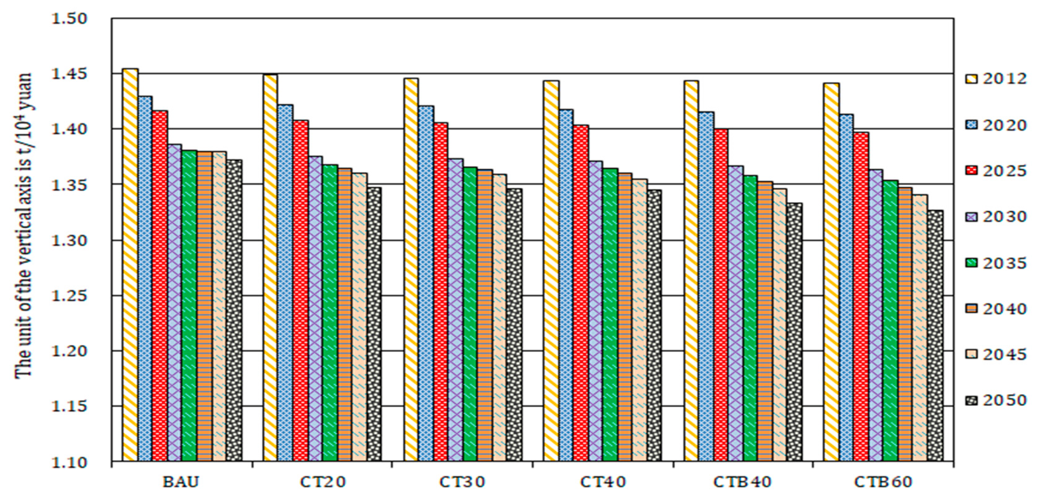[37] whose research introduces carbon tax into China, Meng and Pham [38] whose research introduces carbon tax into the tourism sector in Australia, and Meng [39] whose research focuses on the impact of carbon tax on electricity sector, this article sets up six different scenarios to impose a carbon tax on agriculture-related sectors. Among them, according to the international general experience, the carbon tax should be set gradually in accordance with the low to high, and it is not reasonable to set the carbon tax too high, otherwise the impact on the macroeconomy will be more significant. Scenario 1 is the business as usual (BAU) scenario, in which China does not implement a carbon tax policy between 2012 and 2050. Scenario 2, scenario 3, and scenario 4 can be referred to as CT20, CT30, and CT40 based on the carbon tax rates 20 yuan/ton, 30 yuan/ton, and 40 yuan/ton, respectively. In these scenarios, starting in 2012, the carbon tax rate is increased by 4.33%, 3.22%, and 2.44% per year, respectively, until they each reach 100 yuan/ton in 2050. Scenario 5 and scenario 6, which can be referred to as CTB40 and CTB60, implement balanced tax rates. In scenario 5 and 6, the carbon tax rates are assumed to be 40 yuan/ton and 60 yuan/ton, the indirect production tax is reduced proportionally so that the total tax burden is unchanged. The specific scenarios are shown in

Table 3. The design of different scenarios of imposed carbon tax.

Scenarios	Increasing Rate			Balanced Rate
Tax rate	20	30	40	40	60
BAU	−	−	−	−	−
CT20	+	−	−	−	−
CT30	−	+	−	−	−
CT40	−	−	+	−	−
CTB40	−	−	−	+	−
CTB60	−	−	−	−	+

Note: “+” indicates the given scenario contains the corresponding policy, and “−” indicates that the corresponding measure is not considered.

.

3. Results

3.1. The Changes in Macro-Environment

At present, the world economy is in transition to a low-carbon economy. In this regard, China is also responding positively. In September 2007, China’s National Development and Reform Commission (NDRC) issued the Medium and Long-term Plan of Renewable Energy Source Development to raise the weight of renewable energy to 10%, as a proportion of total primary energy consumption in 2010, and further to 15% in 2020, which is expected to contribute greatly to the objectives of saving about 5–6 billion tons of CO₂ emissions by 2020 [40]. However, despite this situation, China’s current energy structure is still unbalanced compared with the world level, and China’s unbalanced structure results in a series of problems, especially regarding the CO₂ emissions that may hinder sustainable development [41]. This kind of situation is also reflected in agriculture-related sectors. Controlling agricultural CO₂ emissions may not only have a positive impact on the sustainable development of agriculture itself, but it may also make a corresponding contribution to the development of low-carbon agriculture. Based on the GDP forecast in China from 2012 to 2050, this section uses carbon intensity as an indicator to compare the CO₂ emission values of a unit of GDP under different scenarios. Because the indicator of carbon intensity can not only reflect economic condition, but reveal the environmental effects with the development of economy. The results are shown in Figure 2.

In general, if agriculture-related sectors do not impose a carbon tax in the future, carbon intensity will decrease from 1.454 t/10⁴ yuan in 2012 to 1.372 t/10⁴ yuan in 2050, for a total decrease of 5.640%. However, according to the simulation results, the average annual growth rate of CO₂ emissions in the period from 2012 to 2050 is 6.172%, given the rapid growth rate of GDP, which is due to the absence of carbon emission reduction measures. It can be seen from Figure 2 that after the carbon tax is levied, the reduction in the carbon intensity is obviously relative to the scenario without a carbon tax. In the CTB40 and CTB50 scenarios, the reduction of the carbon intensity is more obvious than in the CT20, CT30, and CT40 scenarios. This is mainly because increasing the carbon tax while reducing the indirect production tax in the same proportion will decrease product prices, increase consumer demand for products, enlarge the scale of reproduction, and increase GDP compared to the BAU scenario. At the same time, compared with CT20, CT30, and CT40, the extent of the impact on carbon emissions is greater than the extent of the impact on GDP, so the changes in carbon intensity are more obvious than in the previous three scenarios. In addition, Figure 2 shows that the impact of a carbon tax on China’s carbon intensity gradually weakens as time passes by. Taking CT30 as an example, from 2012 to 2030, the value of carbon intensity varies from 1.446 t/10⁴ yuan to 1.373 t/10⁴ yuan, and the magnitude of the decrease is 5.048%. From 2030 to 2050, the value of carbon intensity varies from 1.373 t/10⁴ yuan to 1.346 t/10⁴ yuan, and the magnitude of the decrease is 1.966%, which is similar to other scenarios. This suggests that the application of a carbon tax policy to reduce CO₂ emissions in agriculture-related sectors has an effect in the short term.

3.2. The Changes in Macroeconomy

The impact of the carbon tax on China’s carbon intensity is mainly through the impacts on GDP and on carbon emissions. Although the effect of reducing the carbon intensity is significant, as an important energy-saving policy, the feasibility of the carbon tax policy depends not only on its emission reduction effect but also on its economic costs. Considering this situation, the six indicators of GDP, CO₂ emissions, households’ consumption, households’ welfare, government expenditure, and investment are selected to reflect the impact of a carbon tax on the macroeconomy. The welfare of the households is mainly measured based on the extent of change in the income level of the households relative to BAU scenario. The specific results are shown in Figure 3 and

Table 4. The changes in macroeconomic indicators under different scenarios between 2012–2050 (%) (compared with the BAU scenario).

Scenarios	Year	GDP	CO2 Emissions	Households’ Consumption	Households’ Welfare	Government Expenditures	Investment
CT20	2012	−0.215	−0.580	−0.184	−0.180	−0.184	−0.419
	2025	−0.358	−0.998	−0.294	−0.287	−0.294	−0.643
	2035	−0.500	−1.443	−0.398	−0.389	−0.396	−0.908
	2050	−0.828	−2.597	−0.598	−0.604	−0.594	−1.443
CT30	2012	−0.311	−0.862	−0.259	−0.254	−0.259	−0.562
	2025	−0.439	−1.250	−0.353	−0.346	−0.353	−0.790
	2035	−0.561	−1.643	−0.438	−0.430	−0.436	−1.022
	2050	−0.930	−2.821	−0.643	−0.633	−0.613	−1.562
CT40	2012	−0.397	−1.119	−0.322	−0.315	−0.322	−0.711
	2025	−0.503	−1.460	−0.399	−0.391	−0.398	−0.912
	2035	−0.621	−1.832	−0.475	−0.469	−0.475	−1.132
	2050	−1.072	−3.043	−0.723	−0.682	−0.662	−1.671
CTB40	2012	0.360	−0.384	0.056	0.118	−0.136	0.631
	2025	0.538	−0.643	0.116	0.196	−0.202	0.793
	2035	0.732	−0.956	0.202	0.291	−0.274	0.945
	2050	1.162	−1.733	0.465	0.523	−0.432	1.229
CTB60	2012	0.437	−0.460	0.101	0.197	−0.105	0.842
	2025	0.647	−0.765	0.210	0.342	−0.157	1.077
	2035	0.874	−1.131	0.368	0.523	−0.214	1.301
	2050	1.373	−2.033	0.854	0.989	−0.339	1.729

Note: all the values are percentage variations; these also apply to all subsequent tables.

.

The results of the simulation show that carbon tax has different effects on key macroeconomic variables in different scenarios. Overall, from the trend point of view, the impacts of carbon tax on CO₂ emissions and government expenditures are similar. With the increase in taxation, CO₂ reduction will be more and more obvious. In addition, emissions and expenditures of CTB40 and CTB60 are lower than those of CT60, but there is still a decreasing trend in CTB40 and CTB60. Moreover, the imposition of carbon tax on agricultural-related sectors will have the same impact trend on GDP, households’ consumption, households’ welfare and investment, which take effect by the impact of market supply and demand. Specifically, from 2012 to 2050, compared with BAU, the percentage changes in government expenditures and CO₂ emissions show reverse bias, and the percent deviation gradually decreases. As shown in Table 4, in the CT20 scenario, in 2012 and 2025, compared with BAU, CO₂ emissions are 0.580% and 0.998% lower, respectively, and the magnitude of decrease is 72.069% compared with BAU. In 2025 and 2035, CO₂ emissions are 0.998% and 1.443% lower, respectively, and the magnitude of decrease is 44.589%, which is in line with the above-mentioned finding that a carbon tax has a positive effect on reducing CO₂ emissions and improving energy efficiency in the short term. In addition, the CT20, CT40, and CT60 scenarios reverse the bias of percentage changes in GDP, households’ consumption, households’ welfare, and investment compared with BAU. However, the CTB40 and CTB60 scenarios show a positive deviation in above indicators compared with BAU. This suggests that if the carbon tax is applied alone, though the effect on CO₂ emissions will be significant, the overall macroeconomy will be sluggish, and the market demand will be depressed. As a result, the level of investment consumption will fall. When imposing a carbon tax and reducing the indirect production tax at the same proportion, due to economic expansion, the domestic market demand for products will increase and the level of investment in goods will also increase, thus stimulating consumer spending and leading to a substantial increase in GDP, as well as welfare.

By comparing the CT20, CT30, and CT40 scenarios, with the change of carbon tax rate ranging from 20 yuan/t to 40 yuan/t, the effect of a carbon tax on macroeconomic variables is becoming more and more obvious. Taking 2050 as an example, compared with BAU, the GDP in the CT20, CT30, and CT40 scenarios is 0.828%, 0.930%, and 1.072% lower, respectively. Carbon emissions are 2.597%, 2.821%, and 3.043% lower, respectively. Households’ consumption is 0.598%, 0.643%, and 0.723% lower, respectively. The trend of households’ welfare, government expenditure and investment are the same as the above indicators. This indicates that as tax rates increase, the degree of impact on macroeconomic variables is more serious. Although a high tax rate will help decrease the carbon intensity, promote energy efficiency, and restructure industries as well as reduce emissions, which are in line with the purpose of the carbon tax levied, it will also cause enormous pressure on the macroeconomy and will ultimately lead to economic depression. Therefore, the objective of a carbon tax policy is to determine the optimal carbon tax with the aim of the maximum reduction in emissions and the least negative impact on the economy. On the contrary, in the balanced tax scenarios of CTB40 and CTB60, increasing the carbon tax will expand the scale of production. The higher the carbon tax is, the lower the production tax is, and the more positive the impact on the economy.

3.3. The Impact of Carbon Tax on Agriculture-Related Sectors

This article mainly focuses on the impact of a carbon tax policy on agriculture-related sectors. Therefore, the results of other departments such as the manufacturing and mining industry, construction industry, transport industry, and service industry are not listed. On the analysis of the macro-environment and the macroeconomic effects of a carbon tax levied on the production process in agriculture-related sectors, this article has elaborated on the positive effect of a carbon tax on emission reduction and the negative effect of a carbon tax on restraining economic development, and it further considers the impact of a carbon tax on the various industries of agriculture. Specifically, 23 different industries related to agricultural activities are considered. As the level of the return on capital will have a direct effect on farmers’ willingness to invest, it will directly determine the future direction of the flow of farmers’ funds with a strong incentive orientation. Moreover, the output levels and income levels in agricultural industries are major concerns of the government and farmers, which are related to the livelihood of farmers. These indicators are also key factors to maintain social stability. Therefore, the effects of the different scenarios on the various agriculture-related sectors are analyzed from those three perspectives: the return on capital, the output level, and the income level.

3.3.1. The Changes in the Return on Capital of Agriculture-Related Sectors

As shown in Figure 4, levying a carbon tax on the production process in agriculture-related sectors will have a significant impact on the return on capital of agriculture-related sectors compared with levying a noncarbon tax. However, different scenarios can generate different positive and negative offsets. As shown in

Table 5. The changes in the return on capital in agriculture-related sectors under different scenarios compared with the BAU scenario (%) (from rice to tea).

Scenarios	Year	Rice	Wheat	Corn	Beans, Potato	Peanut, Rapeseed, Sesame	Cotton, Hemp	Tobacco	Tea
CT20	2012	−0.645	−0.474	−0.602	−0.577	−0.532	−0.329	−0.287	−0.215
	2030	−1.261	−0.862	−1.142	−1.067	−0.971	−0.548	−0.503	−0.289
	2050	−2.635	−1.500	−2.337	−2.014	−1.729	−0.632	−0.515	−0.467
CT30	2012	−0.922	−0.661	−0.854	−0.805	−0.743	−0.477	−0.354	−0.242
	2030	−1.485	−0.983	−1.423	−1.230	−1.111	−0.577	−0.530	−0.308
	2050	−2.911	−1.683	−2.582	−2.223	−1.884	−0.642	−0.531	−0.492
CT40	2012	−1.171	−0.811	−1.014	−0.999	−0.913	−0.534	−0.421	−0.280
	2030	−1.685	−1.085	−1.618	−1.373	−1.228	−0.595	−0.555	−0.324
	2050	−3.175	−1.879	−2.701	−2.443	−2.020	−0.660	−0.550	−0.520
CTB40	2012	−0.503	−0.312	−0.521	−0.493	−0.473	−0.302	−0.243	−0.193
	2030	−1.062	−0.605	−1.004	−0.893	−0.834	−0.416	−0.339	−0.282
	2050	−2.441	−1.265	−2.081	−1.728	−1.564	−0.592	−0.492	−0.432
CTB60	2012	−0.382	−0.283	−0.413	−0.400	−0.398	−0.273	−0.220	−0.169
	2030	−0.857	−0.517	−0.828	−0.759	−0.705	−0.388	−0.316	−0.252
	2050	−2.104	−1.010	−1.795	−1.543	−1.332	−0.572	−0.473	−0.392

,

Table 6. The changes in the return on capital in agriculture-related sectors under different scenarios compared with the BAU scenario (%) (from fruit to vegetables and other processing).

Scenarios	Year	Fruit	Animal Husbandry	Dairy Industry	Forestry	Fishery Industry	Slaughtering and Meat Processing	Animal and Plant Oil Processing	Vegetables and Other Processing
CT20	2012	−1.164	−0.638	−0.801	−1.252	−0.857	0.106	−0.526	−0.451
	2030	−2.299	−1.063	−1.350	−2.145	−1.367	0.125	−1.043	−0.798
	2050	−4.552	−1.862	−2.506	−3.714	−2.070	0.235	−2.079	−1.458
CT30	2012	−1.681	−0.849	−1.062	−1.671	−1.112	0.111	−0.766	−0.616
	2030	−2.697	−1.194	−1.535	−2.435	−1.510	0.150	−1.222	−0.912
	2050	−4.911	−2.064	−2.754	−4.020	−2.220	0.246	−2.281	−1.606
CT40	2012	−2.137	−1.008	−1.274	−2.023	−1.304	0.115	−0.970	−0.751
	2030	−3.046	−1.308	−1.699	−2.693	−1.626	0.169	−1.379	−1.009
	2050	−5.431	−2.275	−3.015	−4.353	−2.391	0.261	−2.490	−1.772
CTB40	2012	−0.954	−0.463	0.402	−1.015	−0.554	0.432	0.701	0.521
	2030	−1.802	−0.728	0.828	−1.772	−0.959	0.699	1.076	0.877
	2050	−3.656	−1.203	1.846	−3.289	−1.763	1.192	1.732	1.563
CTB60	2012	−0.684	−0.310	0.621	−0.732	−0.438	0.633	0.845	0.660
	2030	−1.336	−0.530	1.139	−1.426	−0.765	1.047	1.319	1.059
	2050	−2.813	−0.963	2.232	−2.993	−1.421	1.832	2.163	1.790

and

Table 7. The changes in the return on capital in agriculture-related sectors under different scenarios compared with the BAU scenario (%) (from sugar to wood products).

Scenarios	Year	Sugar	Drinks and Refined Tea	Tobacco Products	Feed processing Industry	Textile	Leather	Wood Products
CT20	2012	−0.580	−0.393	−0.283	−0.248	−0.148	−0.027	−0.417
	2030	−1.017	−0.788	−0.442	−0.529	−0.346	−0.054	−0.824
	2050	−1.773	−1.652	−1.110	−1.160	−0.744	−0.150	−1.605
CT30	2012	−0.790	−0.570	−0.335	−0.372	−0.246	−0.033	−0.599
	2030	−1.154	−0.931	−0.519	−0.634	−0.422	−0.063	−0.966
	2050	−1.910	−1.831	−1.220	−1.280	−0.801	−0.182	−1.737
CT40	2012	−0.959	−0.730	−0.412	−0.487	−0.323	−0.038	−0.765
	2030	−1.271	−1.059	−0.597	−0.726	−0.485	−0.073	−1.088
	2050	−2.052	−2.010	−1.320	−1.411	−0.859	−0.221	−1.871
CTB40	2012	0.743	0.443	0.220	0.260	0.167	0.084	0.491
	2030	1.128	0.767	0.427	0.469	0.317	0.194	0.826
	2050	1.794	1.413	0.892	0.902	0.644	0.493	1.473
CTB60	2012	0.833	0.521	0.264	0.294	0.222	0.102	0.600
	2030	1.308	0.918	0.495	0.552	0.387	0.236	0.956
	2050	2.160	1.724	0.995	1.114	0.721	0.598	1.604

, the five agriculture-related sectors that experience the greatest impact on the return on capital when a carbon tax is levied on the production process are fruit and other planting, forestry, rice planting, the dairy industry, and corn planting. The five industries with the least impact on the return on capital are the leather products industry, tea planting, tobacco planting, cotton, hemp planting, and the textile industry. The main reason for the polarization of the impact on capital return is the difference in carbon emissions between the different industries. A carbon tax on agriculture-related sectors with more carbon emissions will increase the input costs much more than in agriculture-related sectors with less carbon emissions.

By comparing different scenarios according to the positive and negative offsets of the return on capital, the agriculture-related sectors can be roughly divided into two categories. In the first category, the carbon tax has a negative impact on agriculture-related sectors. This category includes rice planting; wheat planting; corn planting; beans and potato planting; peanut, rapeseed, and sesame planting; cotton and hemp planting; tobacco planting; tea planting; fruit and other planting; animal husbandry; forestry; and the fishery industry for a total of 12 industries. In the second category, the CT20, CT30, and CT40 scenarios have negative impacts on the return on capital in the agriculture-related sectors, but the CTB40 and CTB60 scenarios have positive impacts on the return on capital. This category includes 11 agriculture-related industries other than the above 12 industries. The main reason may be that the first category of agriculture-related sectors includes basic agricultural industries, in which the cycle of congenital production is long and supply regulations lag behind changes in market regulations, and the provision of food cannot be substituted. If a carbon tax is levied on those subsidized industries while the indirect production tax is reduced at the same ratio, for the first category of subsidized industries, since these industries are already subsidized by the government, they cannot enjoy the benefits of reducing the indirect taxation. Instead, it will increase the production costs of these subsidized industries. Moreover, it is not conducive to the production of capital accumulation, and will eventually lead to a lower return on capital. For the second category of nonsubsidized industries, the benefits of reducing indirect tax can be mainly applied to these nonsubsidized industries such as the dairy industry, the slaughter and meat processing industry, etc. As a result, these nonsubsidized industries will expand their production scale to lower input costs, improve revenue, and increase the input-output level, ultimately improving the return on capital.

3.3.2. The Changes in the Output Level of Agriculture-Related Sectors

As shown in Figure 5, a carbon tax on agriculture-related sectors will have a significant impact on the output level compared with the non-introduction of a carbon tax, but the impacts vary depending on the specific agriculture-related industry. At the same time, different scenarios generate different positive and negative offsets. As shown in

Table 8. The changes in outputs in agriculture-related sectors under different scenarios compared with the BAU scenario (%) (from rice to tea).

Scenarios	Year	Rice	Wheat	Corn	Beans, Potato	Peanut, Rapeseed, Sesame	Cotton, Hemp	Tobacco	Tea
CT20	2012	−0.159	−0.114	−0.139	−0.136	−0.127	−0.049	−0.037	−0.020
	2030	−0.317	−0.187	−0.296	−0.248	−0.220	−0.064	−0.044	−0.044
	2050	−0.636	−0.249	−0.616	−0.390	−0.286	−0.102	−0.093	−0.094
CT30	2012	−0.231	−0.155	−0.211	−0.191	−0.176	−0.054	−0.039	−0.030
	2030	−0.372	−0.200	−0.356	−0.280	−0.243	−0.071	−0.048	−0.053
	2050	−0.702	−0.278	−0.676	−0.411	−0.288	−0.111	−0.101	−0.103
CT40	2012	−0.294	−0.180	−0.272	−0.234	−0.210	−0.060	−0.042	−0.040
	2030	−0.420	−0.207	−0.411	−0.305	−0.258	−0.078	−0.052	−0.061
	2050	−0.777	−0.309	−0.737	−0.432	−0.292	−0.119	−0.110	−0.113
CTB40	2012	−0.114	−0.090	−0.097	−0.090	−0.091	−0.035	−0.027	−0.015
	2030	−0.213	−0.121	−0.189	−0.149	−0.130	−0.048	−0.040	−0.029
	2050	−0.426	−0.167	−0.396	−0.261	−0.191	−0.069	−0.062	−0.060
CTB60	2012	−0.084	−0.073	−0.077	−0.072	−0.067	−0.026	−0.020	−0.013
	2030	−0.168	−0.094	−0.150	−0.116	−0.096	−0.035	−0.030	−0.024
	2050	−0.365	−0.125	−0.315	−0.196	−0.144	−0.048	−0.047	−0.048

,

Table 9. The changes in outputs in agriculture-related sectors under different scenarios compared with the BAU scenario (%) (from fruit to vegetables and other processing).

Scenarios	Year	Fruit	Animal Husbandry	Dairy Industry	Forestry	Fishery Industry	Slaughtering and Meat Processing	Animal and Plant Oil Processing	Vegetables and Other Processing
CT20	2012	−0.268	−0.128	−0.159	−0.287	−0.110	0.100	−0.230	−0.159
	2030	−0.598	−0.221	−0.294	−0.554	−0.191	0.277	−0.510	−0.309
	2050	−1.313	−0.347	−0.548	−1.015	−0.266	1.008	−1.124	−0.551
CT30	2012	−0.412	−0.175	−0.223	−0.409	−0.151	0.154	−0.355	−0.230
	2030	−0.722	−0.246	−0.338	−0.644	−0.212	0.376	−0.613	−0.358
	2050	−1.438	−0.369	−0.591	−1.086	−0.274	1.164	−1.237	−0.589
CT40	2012	−0.548	−0.210	−0.275	−0.516	−0.181	0.240	−0.468	−0.289
	2030	−0.832	−0.267	−0.376	−0.720	−0.227	0.473	−0.704	−0.398
	2050	−1.564	−0.392	−0.641	−1.160	−0.287	1.323	−1.358	−0.629
CTB40	2012	−0.193	−0.856	0.044	−0.220	0.150	0.392	0.310	0.215
	2030	−0.395	−0.433	0.129	−0.374	0.150	0.778	0.681	0.408
	2050	−0.879	−0.203	0.424	−0.674	0.331	1.665	1.632	0.830
CTB60	2012	−0.141	−0.646	0.072	−0.157	0.188	0.513	0.393	0.272
	2030	−0.293	−0.351	0.200	−0.273	0.188	0.928	0.862	0.528
	2050	−0.661	−0.178	0.620	−0.503	0.450	1.793	2.063	1.103

and

Table 10. The changes in outputs in agriculture-related sectors under different scenarios compared with the BAU scenario (%) (from sugar to wood products).

Scenarios	Year	Sugar	Drinks and Refined Tea	Tobacco Products	Feed Processing Industry	Textile	Leather	Wood Products
CT20	2012	−0.186	−0.198	−0.151	−0.122	−0.040	0.107	−0.263
	2030	−0.396	−0.393	−0.337	−0.217	−0.055	0.407	−0.517
	2050	−0.787	−0.773	−0.721	−0.315	−0.095	1.017	−0.957
CT30	2012	−0.282	−0.289	−0.243	−0.171	−0.046	0.166	−0.379
	2030	−0.469	−0.460	−0.406	−0.242	−0.061	0.546	−0.587
	2050	−0.855	−0.841	−0.781	−0.328	−0.101	1.164	−1.027
CT40	2012	−0.366	−0.366	−0.310	−0.206	−0.052	0.256	−0.481
	2030	−0.531	−0.518	−0.470	−0.260	−0.068	0.680	−0.632
	2050	−0.928	−0.912	−0.842	−0.341	−0.108	1.316	−1.109
CTB40	2012	0.260	0.290	0.190	0.150	0.041	0.452	0.360
	2030	0.522	0.551	0.396	0.255	0.061	0.837	0.683
	2050	1.131	1.123	0.893	0.460	0.095	1.661	1.391
CTB60	2012	0.304	0.351	0.230	0.191	0.050	0.580	0.449
	2030	0.649	0.680	0.504	0.325	0.080	1.015	0.865
	2050	1.506	1.419	1.201	0.590	0.134	1.890	1.791

, the five agriculture-related sectors with the greatest negative impact on the levels of output are fruit and other planting, the animal and plant oil processing industry, forestry, the wood products processing industry, and the sugar products processing industry. The five agriculture-related sectors with the least negative impact on the levels of output are tobacco planting, the textile industry, cotton and hemp planting, tea planting, and the fishery industry. In contrast, the impact of the introduction of a carbon tax on agriculture-related sectors that are subsidized is generally smaller than the impact on nonsubsidized agriculture-related sectors.

In addition, Figure 5 shows that, in the CT20, CT40, and CT60 scenarios, although the slaughter and meat processing industry and the leather products industry have positive deviations from the BAU levels of output, the other 21 agriculture-related sectors show different degrees of negative deviation in the levels of output. This may be due to taxation leading to increased costs for agriculture-related sectors that emit CO₂ into the air, ultimately leading to a rise in the output prices of their agricultural products. In order to avoid the cost of the carbon tax, agriculture-related sectors such as the slaughter and meat processing industry and the leather products industry will promote agricultural CO₂ emissions reduction through technological innovation or changing the mode of production, thus will lead to an increase in output levels of those sectors. However, in other agriculture-related sectors may reduce CO₂ emissions by reducing the scale of production. The former are called technology-intensive industries, and the latter are known as labor-intensive industries. That means that the more labor-intensive agriculture-related sectors are forced, by a carbon tax, to reduce their production scale, resulting in a negative shift in the levels of output in various agriculture-related sectors.

Finally, by comparing the different scenarios shown in Figure 5 and in Table 8, Table 9 and Table 10, it can be seen that the impacts of the different scenarios with offsets, which are positive or negative relative to the output level, are different. The result is the same as with the impact on the return on capital of agriculture-related sectors. The main difference is between subsidized and nonsubsidized industries. It also shows that for subsidized agriculture-related sectors, introducing a carbon tax at the same time as indirect taxes are cut in proportion is not conducive to expanding production.

3.3.3. The Changes in the Income Level of Households in Various Industries of Agriculture

It can be seen from Figure 6 that, subject to the decline in the rate of return on capital and the level of output, the imposition of a carbon tax on agriculture-related sectors will significantly change the income levels of the various industries in agriculture.

Table 11. The changes in the households’ income in agriculture-related sectors under different scenarios compared with the BAU scenario (%) (from rice to tea).

Scenarios	Year	Rice	Wheat	Corn	Beans, Potato	Peanut, Rapeseed, Sesame	Cotton, Hemp	Tobacco	Tea
CT20	2012	−0.216	−0.149	−0.179	−0.189	−0.171	−0.092	−0.073	−0.032
	2030	−0.417	−0.235	−0.272	−0.330	−0.288	−0.145	−0.109	−0.065
	2050	−0.803	−0.611	−0.641	−0.485	−0.354	−0.210	−0.170	−0.142
CT30	2012	−0.310	−0.198	−0.229	−0.260	−0.234	−0.131	−0.106	−0.047
	2030	−0.486	−0.248	−0.305	−0.368	−0.313	−0.159	−0.117	−0.076
	2050	−0.874	−0.671	−0.678	−0.501	−0.365	−0.221	−0.179	−0.156
CT40	2012	−0.389	−0.228	−0.259	−0.313	−0.276	−0.169	−0.136	−0.061
	2030	−0.545	−0.256	−0.333	−0.397	−0.330	−0.173	−0.125	−0.086
	2050	−0.951	−0.732	−0.718	−0.518	−0.376	−0.232	−0.190	−0.171
CTB40	2012	−0.160	−0.107	−0.136	−0.141	−0.123	−0.066	−0.053	−0.024
	2030	−0.278	−0.205	−0.237	−0.217	−0.168	−0.091	−0.075	−0.046
	2050	−0.511	−0.421	−0.439	−0.350	−0.237	−0.129	−0.110	−0.095
CTB60	2012	−0.120	−0.079	−0.105	−0.100	−0.090	−0.049	−0.039	−0.017
	2030	−0.223	−0.150	−0.183	−0.157	−0.124	−0.067	−0.056	−0.034
	2050	−0.441	−0.307	−0.341	−0.260	−0.178	−0.097	−0.086	−0.072

,

Table 12. The changes in the households’ income in agriculture-related sectors under different scenarios compared with the BAU scenario (%) (from fruit to vegetables and other processing).

Scenarios	Year	Fruit	Animal Husbandry	Dairy Industry	Forestry	Fishery Industry	Slaughtering and Meat Processing	Animal and Plant Oil Processing	Vegetables and Other Processing
CT20	2012	−0.215	−0.213	−0.276	−0.339	−0.223	0.221	−0.484	−0.400
	2030	−0.362	−0.363	−0.504	−0.645	−0.387	0.549	−0.907	−0.609
	2050	−0.476	−0.561	−0.939	−1.159	−0.550	1.782	−1.577	−0.704
CT30	2012	−0.290	−0.290	−0.384	−0.480	−0.305	0.318	−0.692	−0.518
	2030	−0.398	−0.403	−0.579	−0.747	−0.430	0.732	−1.037	−0.647
	2050	−0.482	−0.596	−1.020	−1.235	−0.566	2.030	−1.690	−0.709
CT40	2012	−0.345	−0.345	−0.473	−0.602	−0.367	0.403	−0.852	−0.590
	2030	−0.423	−0.436	−0.644	−0.833	−0.463	0.904	−1.145	−0.671
	2050	−0.490	−0.639	−1.103	−1.326	−0.586	2.280	−1.810	−0.716
CTB40	2012	−0.161	−0.166	0.350	−0.260	0.286	0.514	0.653	0.551
	2030	−0.222	−0.247	0.585	−0.424	0.465	1.187	1.112	0.739
	2050	−0.319	−0.384	1.034	−0.730	0.799	3.012	2.010	1.022
CTB60	2012	−0.120	−0.122	0.421	−0.180	0.341	0.661	0.827	0.659
	2030	−0.169	−0.187	0.767	−0.306	0.560	1.498	1.407	0.907
	2050	−0.246	−0.299	1.494	−0.550	0.973	3.722	2.538	1.292

and

Table 13. The changes in households’ income in agriculture-related sectors under different scenarios compared with the BAU scenario (%) (from sugar to wood products).

Scenarios	Year	Sugar	Drinks and Refined Tea	Tobacco Products	Feed Processing Industry	Textile	Leather	Wood Products
CT20	2012	−0.543	−0.335	−0.301	−0.173	−0.069	0.150	−0.406
	2030	−0.879	−0.589	−0.545	−0.276	−0.136	0.407	−0.727
	2050	−1.166	−0.952	−0.871	−0.351	−0.381	1.382	−1.124
CT30	2012	−0.723	−0.463	−0.413	−0.232	−0.091	0.231	0.562
	2030	−0.958	−0.662	−0.622	−0.293	−0.177	0.546	−0.819
	2050	−1.199	−1.013	−0.932	−0.371	−0.451	1.583	−1.175
CT40	2012	−0.843	−0.558	−0.513	−0.267	−0.120	0.355	−0.686
	2030	−1.015	−0.722	−0.682	−0.303	−0.212	0.680	−0.891
	2050	−1.235	−1.082	−0.995	−0.392	−0.517	1.792	−1.231
CTB40	2012	0.604	0.452	0.389	0.210	0.093	0.562	0.510
	2030	0.927	0.731	0.618	0.305	0.217	1.002	0.852
	2050	1.493	1.247	1.033	0.460	0.554	1.903	1.507
CTB60	2012	0.826	0.560	0.494	0.260	0.118	0.693	0.661
	2030	1.228	0.948	0.755	0.384	0.270	1.199	1.106
	2050	1.907	1.702	1.211	0.592	0.676	2.203	1.960

show that the five industries with the greatest negative impacts on the income level after introduction of the carbon tax in agricultural production are the animal and plant oil processing industry, the sugar products processing industry, forestry, the wood products processing industry, and the drinks and refined tea processing industry. In the CT20 scenario in 2020, the corresponding income levels are 1.577%, 1.166%, 1.159%, 1.124%, and 0.952% lower, respectively, compared with BAU, whereas the corresponding rates of return on capital are 2.079%, 1.773%, 3.714%, 1.605%, and 1.652% lower, respectively, compared with BAU, and the corresponding reductions of the output level are 1.124%, 0.787%, 1.015%, 0.957%, and 0.713%, respectively, compared with BAU, which are higher than those of the same index compared with BAU. This indicates that the level of income is closely related to the rate of the return on capital and the level of output.

At the same time, compared with the other scenarios, we find that in the CT20, CT40, and CT60 scenarios, although the income levels of the slaughter and meat processing industry and the leather products industry show a positive deviation, the income levels of the other 21 agriculture-related sectors show different degrees of negative deviation. In addition, in the CTB40 and CTB60 scenarios, the level of income will increase compared with BAU in nonsubsidized agricultural industries, which may be related to a reduction in the production tax resulting in the expansion of the scale of production, increasing production and stimulating consumption.

4. Discussions

4.1. Policy Implications

Through the above analysis, we can see that in order to achieve agricultural CO₂ emissions reductions, we cannot blindly imitate foreign advanced concepts and successful practices. On the contrary, we should combine these concepts with the specific circumstances of the various regions of China, according to local conditions, to explore suitable paths and methods for China’s agricultural CO₂ emissions. Specific practices are as follows:

(1) Find the optimal combination of carbon tax policies.

The simulation results show that levying a carbon tax at the same time as cutting indirect taxes in proportion can reduce the negative impact on agriculture-related sectors. Therefore, the government should determine the carbon tax levied and at the same time set a reasonable carbon tax levy and increase the implementation of transfer payments and other supporting measures to ensure that energy-saving emission reduction measures are effective.

(2) Consider the time effect of the carbon tax.

Given that the effect of the carbon tax in the short term is stronger than in the long term, in the short term, a carbon tax can be the main measure to reduce emissions. In the long term, a carbon tax is as a supplemental tool, and other energy-saving emission reduction methods are the main measures.

(3) Actively explore ways to reduce CO₂ emissions in agriculture-related sectors.

As the results of this study show, due to the natural fragility of China’s agriculture-related sectors, a carbon tax would impose a serious impact on China’s economy of agriculture-related sectors. There is an urgent need to explore other ways to solve the problem of agricultural CO₂ emissions reductions, such as improving energy efficiency or using alternative energy sources, etc., in order to minimize the intensity of the impact on agriculture-related sectors.

As the scope of carbon tax levied mainly due to the combustion of fossil fuels caused by CO₂ emissions, this paper does not consider other CO₂ sources such as pesticide and fertilizer. Finally, the relevant policy recommendations based on the results mainly reflect the impact of the carbon tax levied on the intermediate production process of agricultural-related sectors. Therefore, when considering limiting CO₂ emissions in agricultural-related sectors, on the one hand, tax means can be useful; on the other hand, reducing the intensity of agricultural chemicals, and gradually increasing the input proportion of organic fertilizer, biological pesticides, and other low-carbon green production can limit CO₂ emissions effectively.

4.2. Future Prospects

Although the carbon tax is considered to be one of the most efficient policy means for reducing emissions, it has been controversial about how exactly the carbon tax is levied. Due to the limitations of research conditions, research level, and time, this paper has some of the shortcomings. In the future, efforts and improvements can be made in the following aspects.

(1)

Introduce carbon trading mechanism to make the scenarios more colorful under the premise of the combination of the carbon tax policy and the carbon trading mechanism.

(2)

Further improve the accuracy of the data. Most of the parameters in this model refer to the existing research results. In future research, more detailed data surveys should be conducted to calibrate the parameters more accurately and should be more in line with the characteristics of the real economy.

(3)

Strengthen the model scenarios design to improve the degree of discrimination of carbon tax impacts between different scenarios.

(4)

Update the basic data in a timely manner to improve the accuracy of the results.

5. Conclusions

As a basic industry in China, agriculture has faced more and more problems from CO₂ emissions. Therefore, under the premise of ensuring the stability of China’s agriculture-related economics, formulating effective policy mechanisms to reduce agricultural CO₂ emissions is a serious problem. Based on this situation, this article analyzes the degree of influence of agricultural CO₂ emissions on the macroenvironment, on macroeconomic variables, and on the specific agriculture-related sectors of the 3EAD-CGE model. The conclusions are as follows:

(1)

Whether the short-term and long-term effects of carbon taxes on agriculture-related sectors would be significant if the carbon tax was simply implemented at an incremental rate rather than compensating for the negative effects of carbon taxes. This study provides detailed data that supports the views of most people against the imposition of a carbon tax. From the simulation results, we can see that the capacity in China’s agriculture-related sectors to deal with CO₂ emissions is very fragile. The conclusion of this analysis also verifies why the Chinese government did not adopt the relevant agencies’ recommendations to levy a carbon tax in 2012.

(2)

A policy levying a carbon tax at the same time as cutting indirect taxes in proportion will exert a negative impact on agriculture-related sectors that are subsidized, but the impact is gentler than carrying out a carbon tax alone. From the results of the current model simulations, scenario CTB60 can achieve the best result. However, such a policy is still not conducive to capital accumulation and capital expansion in agriculture-related sectors that are subsidized. In the future development of carbon tax policy, we must carefully consider its impact on the subsidized industries to ensure the output does not decline below China’s base crop yield red line.

References

1. Deng, M.; Li, W.; Hu, Y. Decomposing Industrial Energy-Related CO2 Emissions in Yunnan Province, China: Switching to Low-Carbon Economic Growth. Energies 2016, 9, 23. [Google Scholar] [CrossRef]
2. Vaissiere, A.C.; Levrel, H.; Pioch, S.; Carlier, A. Biodiversity offsets for offshore wind farm projects: The current situation in Europe. Mar. Policy 2014, 48, 172–183. [Google Scholar] [CrossRef]
3. Guan, D.B.; Barker, T. Low-carbon development in the least developed region: A case study of Guangyuan, Sichuan province, southwest China. Nat. Hazards 2012, 62, 243–254. [Google Scholar] [CrossRef]
4. Liobikiene, G.; Butkus, M. The European Union possibilities to achieve targets of Europe 2020 and Paris agreement climate policy. Renew. Energy 2017, 106, 298–309. [Google Scholar] [CrossRef]
5. Lu, J.; Fan, W.; Meng, M. Empirical Research on China’s Carbon Productivity Decomposition Model Based on Multi-Dimensional Factors. Energies 2015, 8, 3093–3117. [Google Scholar] [CrossRef] [Green Version]
6. Gao, C.K.; Wang, D.; Zhao, B.H.; Chen, S.; Qin, W. Analyzing and forecasting CO2 emission reduction in China’s steel industry. Front. Earth Sci. 2015, 9, 105–113. [Google Scholar] [CrossRef]
7. China Daily. China Likely to Levy Carbon Tax Around 2012[EB/OL]. Available online: http://www.chinadaily.com.cn/china/2010-05/11/ content_9834525.htm (accessed on 6 September 2010).
8. IPCC. Climate Change 2007: Impacts, Adaptation and Vulnerability; Cambridge University Press: New York, NY, USA, 2007. [Google Scholar]
9. Food and Agriculture Organization of the United Nations (FAOSTAT). FAO Statistical Yearbook 2013[EB/OL]. Available online: http: //www.fao.org/economic/ess/ess-publications/ess-yearbook/en/ (accessed on 21 August 2015).
10. National Bureau of Statistics (NBS). China Statistical Yearbook 2013; China Statistics Press: Beijing, China, 2015.
11. National Bureau of Statistics (NBS). Input-output Tables of China 2012; China Statistics Press: Beijing, China, 2015.
12. Dong, H.M.; Li, Y.E.; Tao, X.P.; Li, N.; Zhu, Z.P. China greenhouse gas emissions from agricultural activities and its mitigation strategy. Trans. Chin. Soc. Agric. Eng. 2008, 24, 269–273. [Google Scholar]
13. Iodice, P.; Senatore, A. Atmospheric pollution from point and diffuse sources in a National Interest Priority Site located in Italy. Energy Environ. 2016, 27, 586–596. [Google Scholar] [CrossRef]
14. Abagnale, C.; Cardone, M.; Iodice, P.; Strano, S.; Terzo, M.; Vorraro, G. Power requirements and environmental impact of a pedelec. a case study based on real-life applications. Environ. Impact Assess. Rev. 2015, 53, 1–7. [Google Scholar] [CrossRef]
15. Armaroli, N.; Balzani, V. Towards an electricity-powered world. Energy Environ. Sci. 2014, 4, 3193–3222. [Google Scholar] [CrossRef]
16. Charles, D. Stimulus gives DOE billions for carbon-capture projects. Science 2009, 323, 1158. [Google Scholar] [CrossRef] [PubMed]
17. Iodice, P.; Langella, G.; Amoresano, A. Ethanol in gasoline fuel blends: Effect on fuel consumption and engine out emissions of SI engines in cold operating conditions. Appl. Therm. Eng. 2018, 130, 1081–1089. [Google Scholar] [CrossRef]
18. Kitwiwattanachai, A.; Nelson, D.; Reed, G. Quantitative impacts of alternative East Asia free trade areas: A computable general equilibrium (CGE) assessment. J. Policy Model 2010, 32, 286–301. [Google Scholar] [CrossRef]
19. Bor, Y.J.; Huang, Y. Energy taxation and the double dividend effect in Taiwan’s energy conservation policy-an empirical study using a computable general equilibrium model. Energy Policy 2010, 38, 2086–2100. [Google Scholar] [CrossRef]
20. Hermeling, C.; Löschel, A.; Mennel, T. A new robustness analysis for climate policy evaluations: A CGE application for the EU 2020 targets. Energy Policy 2013, 55, 27–35. [Google Scholar] [CrossRef]
21. Mittal, S.; Dai, H.C.; Fujimori, S.; Masui, T. Bridging greenhouse gas emissions and renewable energy deployment target: Comparative assessment of China and India. Appl. Energy 2016, 166, 301–313. [Google Scholar] [CrossRef]
22. Qi, T.Y.; Winchester, N.; Karplus, V.J.; Zhang, D.; Zhang, X.L. An analysis of China’s climate policy using the China-in-Global Energy Model. Econ. Model. 2016, 52, 650–660. [Google Scholar] [CrossRef]
23. Mahmood, A.; Marpaung, O.P. Carbon pricing and energy efficiency improvement—Why to miss the interaction for developing economies? An illustrative CGE based application to the Pakistan case. Energy Policy 2014, 67, 87–103. [Google Scholar] [CrossRef]
24. Markandya, A.; Antimiani, A.; Costantini, V.; Martini, C.; Palma, A.; Tommasino, M.C. Analyzing Trade-offs in International Climate Policy Options: The Case of the Green Climate Fund. World Dev. 2015, 74, 93–107. [Google Scholar] [CrossRef]
25. Springmann, M.; Zhang, D.; Karplus, V.J. Consumption-Based Adjustment of Emissions-Intensity Targets: An Economic Analysis for China’s Provinces. Environ. Resour. Econ. 2015, 61, 615–640. [Google Scholar] [CrossRef]
26. Dong, Y.; Ishikawa, M.; Hagiwara, T. Economic and environmental impact analysis of carbon tariffs on Chinese exports. Energy Econ. 2015, 50, 80–95. [Google Scholar] [CrossRef]
27. Carlos, B.; Luis, G.; Manuel, D.; Rodrigo, F.; Gonzalo, G.; Rodrigo, P.; Catalina, R. The Impact of a Carbon Tax on the Chilean Electricity Generation Sector. Energies 2015, 8, 2674–2700. [Google Scholar] [Green Version]
28. Yang, L.; Yao, Y.F.; Zhang, J.T.; Zhang, X.; McAlinden, K.J. A CGE analysis of carbon market impact on CO2 emission reduction in China: A technology-led approach. Nat. Hazards 2016, 81, 1107–1128. [Google Scholar] [CrossRef]
29. Diao, X.S.; Kennedy, A. Economywide Impact of Maize Export Bans on Agricultural Growth and Household Welfare in Tanzania: A Dynamic Computable General Equilibrium Model Analysis. Dev. Policy Rev. 2016, 34, 101–134. [Google Scholar] [CrossRef]
30. Wiebe, K.; Lotze-Campen, H.; Sands, R.; Tabeau, A.; van der Mensbrugghe, D.; Biewald, A.; Bodirsky, B.; Islam, S.; Kavallari, A.; Mason-D’Croz, D.; et al. Climate Change Impacts on Agriculture in 2050 under a Range of Plausible Socioeconomic and Emissions Scenarios. Available online: http://iopscience.iop.org/article/10.1088/1748-9326/10/8/085010 (accessed on 1 September 2015).
31. Editorial board of China’s financial yearbook. Finance Yearbook of China 2013; China State Finance Magazine: Beijing, China, 2014.
32. Liu, S.J. The Survey of China’s per Capita Income in 2013[EB/OL]. Available online: http://www.chinairn.com/news/20130327/095807960.html (accessed on 27 March 2013).
33. Wang, K.; Wang, C.; Chen, J. Analysis of the economic impact of different Chinese climate policy options based on a CGE model incorporating endogenous technological change. Energy Policy 2013, 37, 2930–2940. [Google Scholar] [CrossRef]
34. China’s Population Development Strategy Research Group, 2007[EB/OL]. Available online: http://www.gov.cn/gzdt/2007-01/11/content_493677.htm> (accessed on 11 January 2007).
35. Pan, H.R. Computable General Equilibrium Model Primary Tutorial, 1st ed.; China Population Publishing House: Beijing, China, 2016. [Google Scholar]
36. Dai, H.C.; Masui, T.; Matsuoka, Y.; Fujimori, S. Assessment of China’s climate commitment and non-fossil energy plan towards 2020 using hybrid AIM/CGE model. Energy Policy 2011, 39, 2875–2887. [Google Scholar] [CrossRef]
37. Li, W.; Li, H.; Sun, S. China’s Low-Carbon Scenario Analysis of CO2 Mitigation Measures towards 2050 Using a Hybrid AIM/CGE Model. Energies 2015, 8, 3529–3555. [Google Scholar] [CrossRef]
38. Meng, S.; Pham, T. The impact of the Australian carbon tax on the tourism industry. Tourism Econ. 2017, 23, 506–522. [Google Scholar] [CrossRef]
39. Meng, S. How may a carbon tax transform Australian electricity industry? A CGE analysis. Appl. Econ. 2014, 46, 796–812. [Google Scholar] [CrossRef]
40. Zhang, D.H.; Wang, J.Q.; Lin, Y.G.; Si, Y.L.; Huang, C.; Yang, J.; Huang, B.; Li, W. Present situation and future prospect of renewable energy in China. Renew. Sustain. Energy Rev. 2017, 76, 865–871. [Google Scholar] [CrossRef]
41. Zhao, X.; Luo, D.K. Driving force of rising renewable energy in China: Environment, regulation and employment. Renew. Sustain. Energy Rev. 2017, 68, 48–56. [Google Scholar] [CrossRef]
Figure 1. General structure of the economy-energy-environmental-agricultural-dynamics CGE model (3EAD-CGE) model in Chinese agriculture-related sectors.
Energies 11 02296 g001
Figure 2. The trend in China’s carbon intensity change under different scenarios.
Energies 11 02296 g002
Figure 3. The trend of China’s macroeconomy under different scenarios (compared with the BAU scenario).
Energies 11 02296 g003
Figure 4. The change in the return on capital in agriculture-related sectors under different scenarios in 2050 (compared with the BAU scenario).
Energies 11 02296 g004
Figure 5. The changes in the outputs in agriculture-related sectors under different scenarios (compared with the BAU scenario).
Energies 11 02296 g005
Figure 6. The changes in the households’ income in agriculture-related sectors under different scenarios (compared with the BAU scenario).
Energies 11 02296 g006