Variable Parameters for a Single Exponential Model of Photovoltaic Modules in Crystalline-Silicon


1
Faculty of Engineering, University of Central Punjab, Lahore 54590, Pakistan
2
Department of Electronics and Telecommunication, Politecnico di Torino, 10129 Torino, Italy
3
Department of Energy, Politecnico di Torino, 10129 Torino, Italy
*
Author to whom correspondence should be addressed.
Energies 2018, 11(8), 2138; https://doi.org/10.3390/en11082138
Submission received: 18 July 2018
/
Revised: 8 August 2018
/
Accepted: 13 August 2018
/
Published: 16 August 2018
(This article belongs to the Special Issue Sustainable Energy Systems)
Abstract
:The correct approximation of parallel resistance (Rp) and series resistance (Rs) poses a major challenge for the single diode model of the photovoltaic module (PV). The bottleneck behind the limited accuracy of the model is the static estimation of resistive parameters. This means that Rp and Rs, once estimated, usually remain constant for the entire operating range of the same weather condition, as well as for other conditions. Another contributing factor is the availability of only standard test condition (STC) data in the manufacturer’s datasheet. This paper proposes a single-diode model with dynamic relations of Rp and Rs. The relations not only vary the resistive parameters for constant/distinct weather conditions but also provide a non-iterative solution. Initially, appropriate software is used to extract the data of current-voltage (I-V) curves from the manufacturer’s datasheet. By using these raw data and simple statistical concepts, the relations for Rp and Rs are designed. Finally, it is proved through root mean square error (RMSE) analysis that the proposed model holds a one-tenth advantage over numerous recently proposed models. Simultaneously, it is low complex, iteration-free (0 to voltage in maximum power point Vmpp range), and requires less computation time to trace the I-V curve.
1. Introduction
In the recent era, Photovoltaic (PV) plants, an integral renewable source, have gained enormous popularity around the world [1]. Even developing countries are striving hard to exploit the extensive potential of the PV source [2]. A robust PV model is essential to assess the performance and efficiency of plant [3]. The model can also play an important role in deciding the economic viability, tariff analysis, and pay-back time of investments.
A maximum power point tracking (MPPT) technique, an indispensable element of the system, utilizes the PV model to inspect the different aspects of PV systems such as design issues, electronic interface topologies, the working principle, and control schemes of algorithms [4]. As a result, a PV simulator based on an accurate and fast PV model is required [4,5]. Moreover, the simulator provides a facility to compare the goodness of MPPT algorithms under the same ambient weather conditions [6]. In general, the high complexity of the model ensures high accuracy. Compared to dual-diode and complex models, a single-diode PV model offers the following benefits: (1) It provides a good compromise between accuracy and simplicity, and (2) This model requires less computational burden, time, and cost to produce the I-V curves. The work presented in this paper adopts a single diode model, and the main aim is to enhance the accuracy of the model and its adaptability for a vast range of weather conditions. The mathematical relation of this model is presented in (1):
in which Iph is the photo-generated current due to incident photons on the PV module, Io is the reverse saturation current, and I and V are the output current and voltage, respectively. Rs is the series resistance, which accounts for the voltage drop across the module terminals, while Rp is the parallel resistance, which explains the leakage current along the lateral surfaces of the cells. The thermal voltage (VT) of the module is equal to Nss × nkT/q, in which Nss represents the number of series connected cells in a module, q is the electron charge (1.60217646 × 10⁻¹⁹ C), and k is the Boltzmann constant (1.3806503 × 10⁻²³ J/K), while n states the diode ideality factor.
The fundamental relation (1) of the single-diode model demands five parameters to be evaluated [7,8], in which the introduction of Rs and Rp resistances transforms the ideal model into a practical model. Naturally, correct and sound estimations of these parameters are vital to match the behavior of the practical PV modules. Otherwise, the model may not appropriately replicate the I-V curves of the practical PV modules. Researchers in the past formularized these parameters using three different methods: non-iterative, iterative, and artificial intelligence [9].
Model [10] estimates resistive parameters by considering three remarkable points of the I-V curve: the open-circuit point (OCP), the short-circuit point (SCP), and the maximum power point (MPP), while model [11] evaluates the same parameters through rigorous mathematical calculations. These models are non-iterative and reliable under STC; however, they tend to struggle for remaining weather conditions.
Keeping in view higher model accuracy, the progress in identification of these critical parameters has been recently executed by elite researchers. A reverse identification approach is employed in [7] to extract the key parameters through transitional formulas. The solution is quite effective compared to previous models [10,11]; however, it requires the Newton-Raphson method and the least square method, making it an iterative solution.
A shuffled frog leaping algorithm is outlined in [12] to establish the n, Rs and Rp values of the single-diode model. The complex procedures such as fitness function, random numbers implementation, and iterations are the main drawbacks of this solution. A five parametric model is first converted to the reduced model in [13]. Then, a convex, solution-based optimization and a modified barrier function are involved in the extraction of parameters, establishing it as a highly complex solution.
An intensive scanning with very small steps is adopted in [4] to optimize the n and Rs. Since Rp is estimated through simplified assumption, such a solution is not effective at low irradiance conditions [7]. An attempt is being made to produce a simple and straightforward solution in [3], which utilizes five explicit expressions. Nevertheless, the correlation procedure requires Lambert-W function. The same function is utilized in [14] to state the explicit expressions and Newton–Raphson method is employed for iterations. Note that these models require more computation time to execute the I-V curves. Usually, these models do not update the values of Rs and Rp parameters on a consistent basis owing to varying weather conditions. Consequently, their accuracy decays with changing weather conditions.
On the other hand, genetic algorithm and particle swarm optimization-based schemes are proposed in [15,16], respectively, to determine the Rp and Rs of the single diode model. A reduced, space-based idea is presented in [1], where an experimental curve is scanned to gauge the parameters. These models exhibit good accuracy, but their procedures are highly complex, and their computation cost is significant.
After a comprehensive literature survey of single diode models [9], the following critical observations are noted:
- Since the manufacturer’s datasheet provides STC data only, most models tend to extract parameters from these data, causing the following drawbacks to occur:
- -
- They produce accurate I-V curves under STC, while their performance decays for other irradiance conditions, especially at low irradiance levels;
- -
- Even under STC, some models produce better I-V curves near the MPP region, while the accuracy of curves degrades in other regions;
- -
- Rp and Rs are estimated through either extensive iterative methods or advanced, intelligent schemes, which increase the burden of computation time and complexity, while non-iterative methods are less accurate.
- The core issue in the past proposed models is the static approximation of resistive parameters, in which Rp and Rs, once estimated at STC, not only remain constant around STC but the same values of Rp and Rs are adopted for other conditions, as, for example, with low irradiance (200 W/m2). Thus, models lacked an adaptive ability with varying irradiance levels:
- -
- The above-mentioned point is a major reason for the development of more complex models such as double diode and dynamic models;
- -
- It is also observed that, because of static Rp and Rs values, the models tend to give unrealistic large negative values at open-circuit voltage.
Concerning the drawbacks mentioned above and the gap present in literature, the proposed model entails a new philosophy of dynamic estimations of Rp and Rs. Through this philosophy, the accuracy of the single diode model is enhanced for various weather conditions. In (1), the philosophy of the proposed mechanism is illustrated, and its mathematical representation is indicated in (2) and (3). Initially, a unique idea has been employed to extract the high-resolution data of I-V curves of distinct irradiance levels from the manufacturer’s datasheet. A computer-aided design (CAD) software, i.e., AutoCAD, is used for this purpose. Thereafter, the dynamic estimation of resistive parameters is carried out through three factors: (1) data-mining of I-V curves database, (2) PV parameters, and (3) simple statistical concepts. The expressions of resistive factors contain adaptability for both dynamic/static weather conditions and, simultaneously, they are iteration-free.
The proposed solution is compared with numerous recently proposed models. The proposed model comprehensively outperforms these hi-tech models. At the same time, the proposed solution is fast, simple, and iteration free from 0 to Vmpp.
2. Mathematical Model of PV Module
The mathematical model of proposed method is based on a single diode model, as shown in Figure 1, and is mathematically explained by (1). As is well-known, this model prompts five unknown parameters: Iph, Io, n, Rs, and Rp. The diode ideality factor ‘n’ is a fitting parameter, which determines how close the I-V characteristic of diode is to ideal. A factor of ‘1’ makes its ideal, which assumes that no recombination takes place in the space-charge region. Since solar cells are considerably larger than traditional diodes, most of them exhibit ideal behavior at STC condition, i.e., n ≈ 1. When recombination dominates, the value of n becomes 2. Therefore, it is reasonable to use values within the range from 1 to 2 for model fitting of the experimental I-V points. From a modeling perspective, the value of n is arbitrarily chosen between 1 and 2. Numerous authors suggested distinct ways to estimate the value of n [17,18,19]. However, the proposed model initializes the model with n = 1 [20], and later one readjusts the value on n to increase the accuracy of the model.
The other two current parameters are relatively easier to solve, while a substantial challenge is the estimation of two resistance parameters.
2.1. Determination of Current Parameters
The short-circuit current (Isc) of module relies linearly on solar irradiance (G) and is slightly influenced by the temperature change (∆T), as indicated in the following relation [21,22]:
in which Isc,stc and α represent short-circuit current and temperature coefficient of Isc at STC, respectively. Both can be obtained from manufacturer’s datasheet. Additionally, GSTC and G represent the solar irradiance values at STC and present conditions, respectively. The value of G is measured in W/m2.
Generally, the Iph = Isc is considered a sound assumption for a single diode model [20]. The photo-generated current (Iph) by the current source can be accurately assessed as the short circuit current calculated across the PV cell terminals. Actually, the current divider between a series resistance of hundreds of milliohms and a parallel resistance of hundreds of ohms is dominated by the series resistance, taking into account the practical opening of the diode in the equivalent circuit with zero output voltage. The saturation current (Io) depends on the intrinsic properties of PV cells present in a module such as diffusion coefficient of electrons in the semi-conductor, lifetime of minority carriers, and intrinsic current density, etc [23]. Commercial vendors do not provide such minute details in the datasheets. This paper considers the same indirect relation to measure Io as reported in [23]. Consider open-circuit configuration of the module under STC, in which V = Voc and I = 0; neglecting the leakage current Voc/Rp, (1) can be transformed to find Io as
2.2. Determination of Resistance Parameters
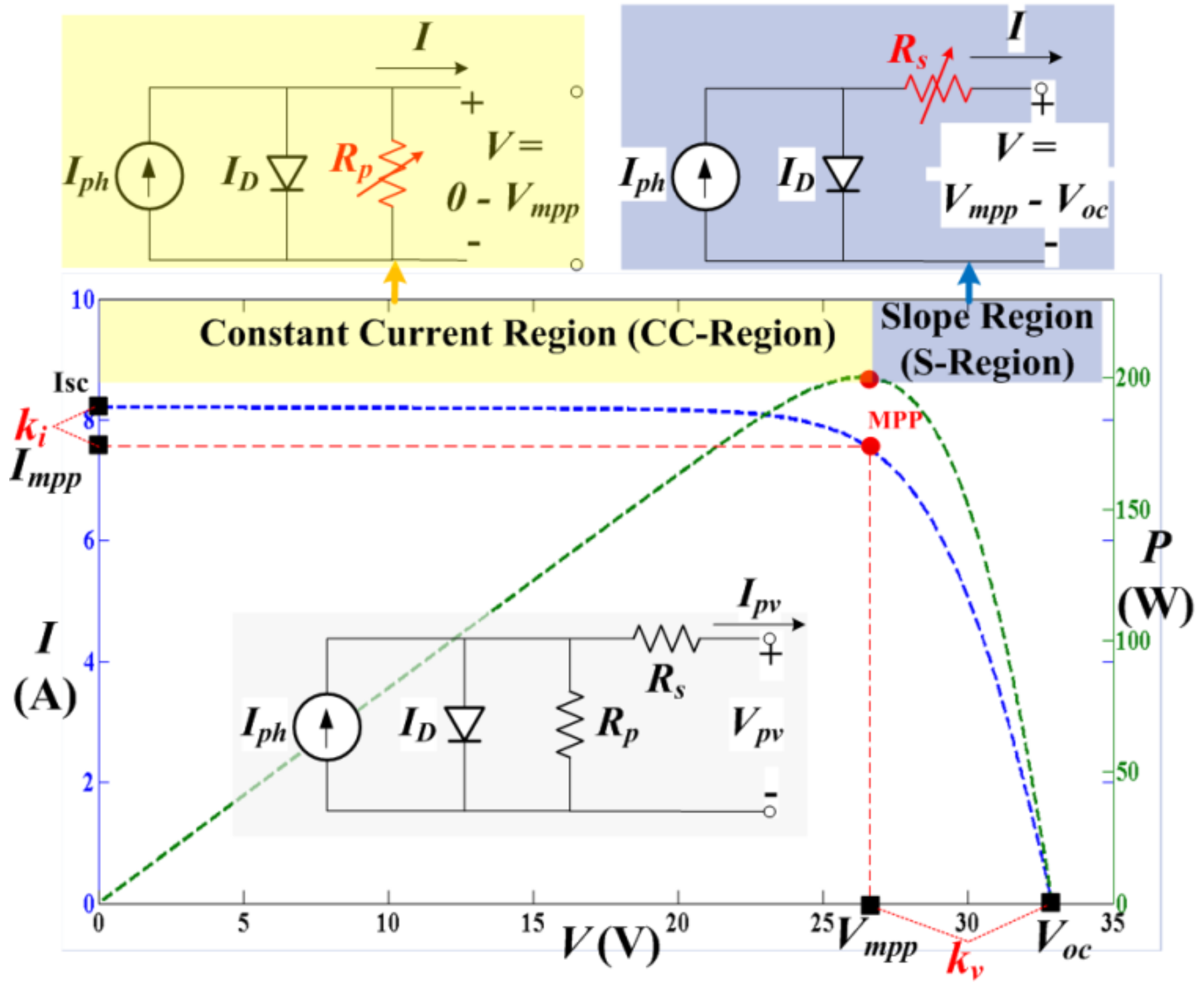
In order to determine Rp and Rs, the proposed model partitions the I-V curve into two regions: (1) from Isc (V = 0) to MPP point, i.e., constant current region (CC-R) and (2) from MPP point to Voc (I = 0), i.e., slope region (S-R), as appeared in Figure 1. In CC-R, Rs is supposed to be zero and Rp is estimated, while in S-region, Rp is considered as infinite and Rs is calculated.
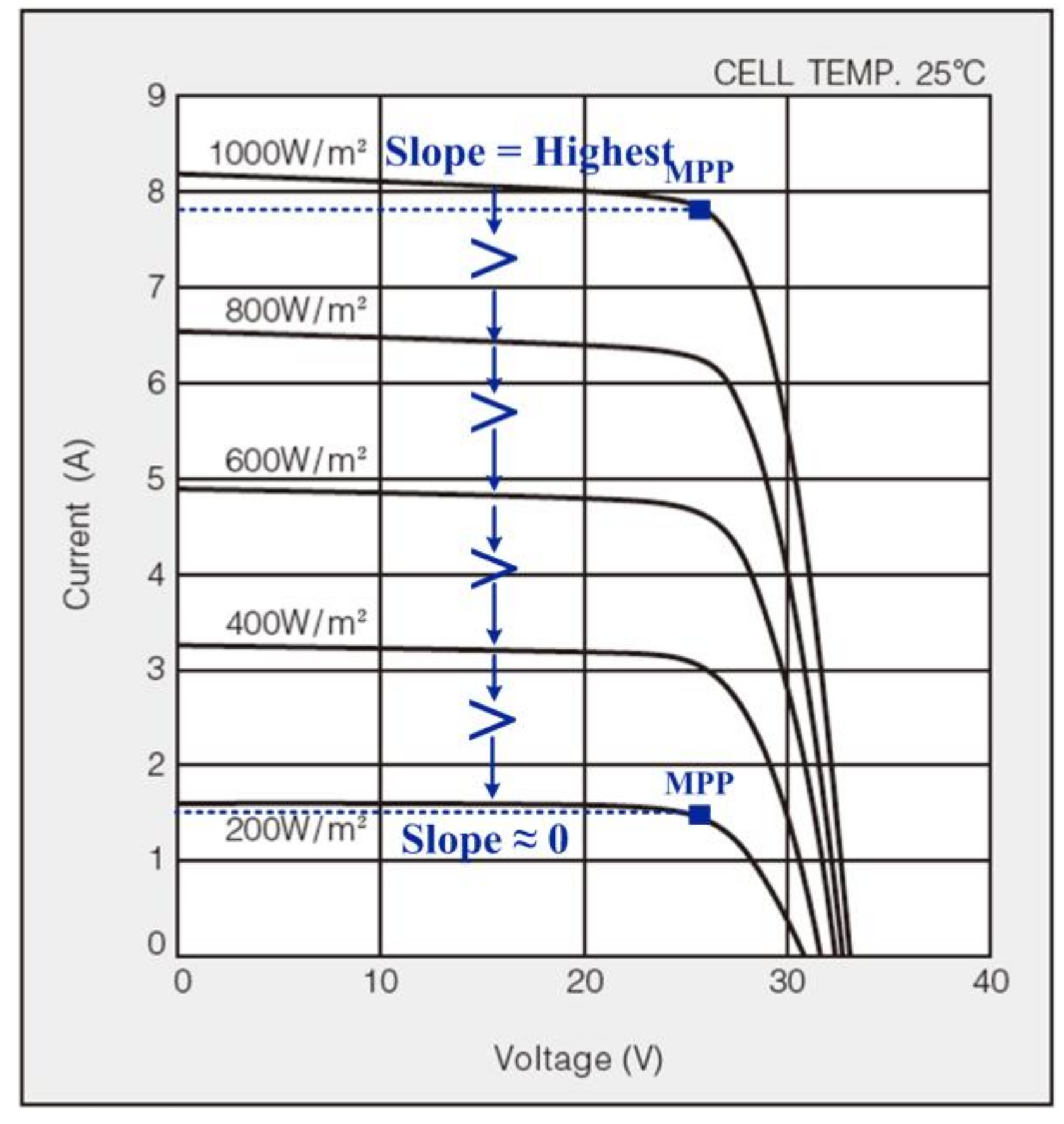
Consider the I-V curves of a multi-crystalline (also defined poly-crystalline) PV module at different irradiance levels presented in Figure 2. It can be observed that the slope of I-V curve in constant current region (CC-R) changes as irradiance level falls from STC. At higher irradiance levels, the slope of I-V curves is greater than the slope of curves at lower irradiance. In fact, at lower irradiance such as 200 W/m2, the slope almost remains constant. With this observation, it is logical to conclude that Rp and Rs should be dynamic with varying irradiance levels. However, the main obstacle in dynamic estimations of resistive parameters is the insufficient information available in manufacturer’s datasheet.
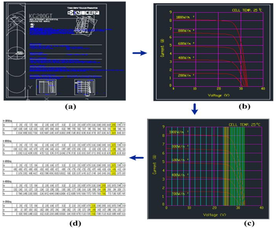
2.2.1. Data-Mining Using CAD Software
The I-V curves at different irradiance levels are difficult to analyze as no clarity for scale and precise tool for accurate measurement is present in portable document format (PDF) software, hence making it inconvenient for the designing of I-V models and I-V simulations to be verified. To get the data out of these raw curves, it has to be processed for better measurement of the I-V values. This is achieved using PDF with computer aided design (CAD) converter, in which datasheet page containing the I-V curve is imported and processed by the software.
In Figure 3a, the form of data sheet after conversion into CAD is represented. Since the data of only I-V curves are required, an exercise is performed for removing all other data from the converted CAD document. For this purpose, AutoCAD application is utilized. Unwanted data are deleted, and only the curves data stayed in CAD for further processing. In Figure 3b, the appearance of curves after removal of unnecessary information is shown. These data contain the information of five curves at different irradiance values, i.e., 1000 W/m2, 800 W/m2, 600 W/m2, 400 W/m2, and 200 W/m2.
The last step of this data processing is the scaling of these curves as per actual dimensions and measurements, as shown in Figure 3c. This exercise converted the cluttered data into a more comprehensible, readable, and presentable form. Finally, the data obtained are ready for data mining and information extraction as required. Figure 3d demonstrates final furnished form of the processed data in a spreadsheet file.
2.2.2. Estimation of Rp Value
To find Rp, its value is estimated using the MPP data. Let us consider MPP variables and, as already mentioned, that in CC-R, the proposed model considers Rs as zero, (1) can be rearranged to find Rp_mpp as
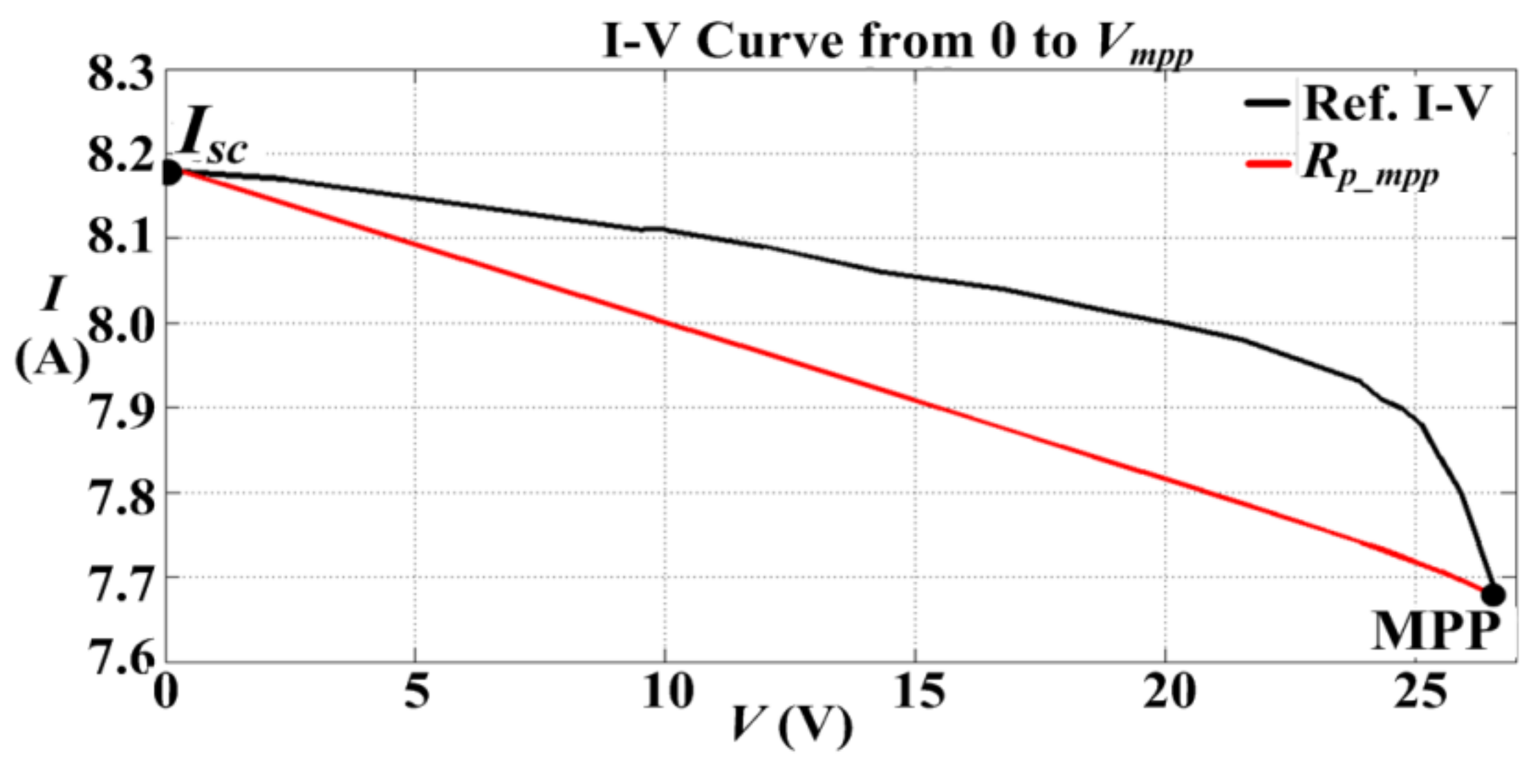
Figure 4 displays two I-V curves from Isc to MPP: The first curve corresponds to STC data (extracted from CAD software), and the second curve is plotted using (1). Here, Rs is assumed as zero; Io = 4.079 × 10⁻¹⁰ A and Rp_mpp = 62.3903 Ω are calculated from (5) and (6), respectively, using the STC data of multicrystalline photovoltaic module. It is obvious that the error at two extreme points (V = 0 and V = Vmpp) is zero. Apart from these two points, the two curves are mismatched, thus highlighting the inaccurate estimation of Rp.
As seen from Ref. I-V curve in Figure 4, I is comparatively large before the MPP region, which implies that Rp is also high in this region. Moreover, while tracing the I-V curve from Isc towards MPP, value of Rp continues to decline until it becomes equal to Rp_mpp at MPP. This observation leads to two considerations: (1) An additional resistive factor (Rp_Est) needs to be incorporated in Rp_mpp, which has more weightage near Isc point and zero weightage at MPP and (2) A mathematical operation is required, which makes the combination of Rp_Est and Rp_mpp dynamic while it moves from Isc to Vmpp. To fulfill the latter consideration, the proposed model utilizes the statistical concept of weighted mean, the generalized formula of which is indicated in (7):
in which x is the value of function parameter and w is the relative weight for the parameter Rp, which empirically adjusts the value of Rp on each operating point of I-V curve. In physical interpretation, it represents the ∆Rp of Rp from one operating point to another point on I-V curve. The above formula is transformed to find out the dynamic Rp_model value as
Let us consider that Rp_Est is estimated, and since Rp_mpp and Vmpp are fixed for a given condition, the only variable that makes Rp_model dynamic is w1, i.e., (Vmpp–V). For instance, at V = Vmpp, Equation (8) leads to Rp_model = Rp_mpp as w1 = 0. On the other hand, the movement of V towards Isc increases, and the weight of Rp_Est increases, which makes the value of Rp_model higher. For example, at V = 0, both Rp_Est and Rp_mpp contributed to Rp_model with equal weights (w1 = Vmpp, and w2 = Vmpp).
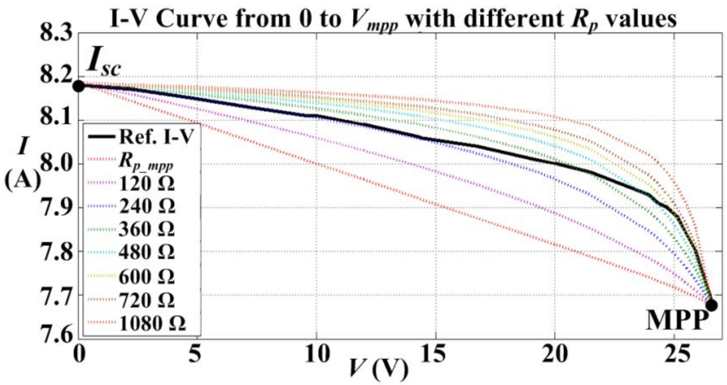
To estimate the Rp_Est, the condition of short-circuit is considered, in which the value of Rp_Est matters the most. Equation (8) implies that when V = 0, Rp_model becomes 0.5 × (Rp_Est + Rp_mpp), which gives an initial clue that Rp_Est should be significantly higher than Rp_mpp in order to settle a much higher Rp_model. Since Rp_mpp ≈ 60 Ω is known quantity from (6), the Rp_Est is estimated with integral multiples of Rp_mpp, i.e., 120 Ω, 240 Ω, 360 Ω, 480 Ω, 600 Ω, 720 Ω, and 1080 Ω. Using these values of Rp_Est, the corresponding Rp_model values are calculated from (8), and I-V curves are sketched from (1).
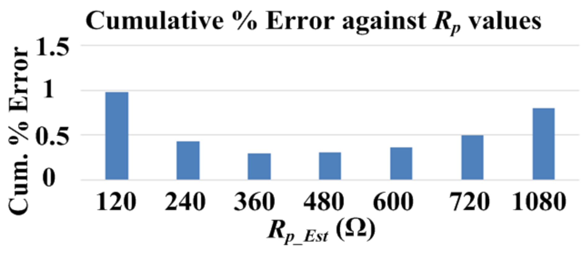
These curves are compared with the Ref. I-V curve (extracted from CAD software) that appears in Figure 5. It can be seen that the curves with Rp_Est of 360 Ω and 480 Ω values (significantly higher than Rp_mpp) depict excellent resemblance with Ref. I-V curve. However, if Rp_Est increases, i.e., 720 Ω, 1080 Ω, the I-V curves once again start diverging from Ref. I-V curve. To further illustrate this matter, Figure 6 gives an indication about the cumulative percent error. It can be noticed that the error starts to reduce from 240 Ω, while it rises once again at higher values. The values between 360 Ω and 480 Ω can be considered as optimum Rp_Est values.
Rp_Est can be calculated from the ratio Voc/Isc. The value turns out to be 4.04 at STC data, which is not the final value but assists in providing a final solution to estimate Rp_Est. Since the optimum range of RP_Est hovers between 360 Ω and 480 Ω, as shown in Figure 6, a factor of 100 is then multiplied with the ratio Voc/Isc to put the RP_Est within the range of 360 Ω to 480 Ω. This factor is not a unit conversion and is introduced based on the calculation of percentage error. To set the Rp_Est, the expression is
in which Isc and Voc values for different environment conditions can be calculated from (4) and the following equation, respectively:
in which β is the temperature coefficient of Voc. By substituting Rp_mpp from (6) and Rp_Est from (9) in (8), the benchmark formula to calculate Rp_model is
Since Voc and Isc values vary with weather conditions, the above Rp_model expression contains adjusting ability through Rp_Est = (Voc/Isc × 100). On the other hand, for steady condition, weighted mean adjusts the I-V curve over a complete range. Besides that, Impp and Vmpp can be computed from Isc and Voc using the following two relations, respectively:
Values of Isc and Voc can be formulated for different weather conditions using (4) and (10), respectively. At STC, the values of coefficients ki and kv can be pre-determined from manufacturer`s datasheet. To find values of these coefficients at various weather conditions, the data extracted from CAD software are utilized. The values of ki for different irradiance levels are numerically found as 0.94@1000 W/m2, 0.93@800 W/m2, 0.92@600 W/m2, 0.93@400 W/m2, and 0.93@200 W/m2. On the other hand, the values of kv are found as: 0.81@1000 W/m2, 0.82@800 W/m2, 0.83@600 W/m2, 0.82@400 W/m2, and 0.82@200 W/m2. Since ki and kv values are similar for different irradiance levels, the proposed model estimates ki and kv from STC information available in datasheet.
2.2.3. Estimation of Rs Value
As already mentioned, the proposed model considers infinite value of Rp from MPP to Voc point, as indicated in Figure 1. Consequently, (1) can be re-arranged to find the Rs value as:
The above equation can be transformed to find Rs value at MPP as
While moving from MPP to Voc, the Rs value should reduce and eventually become zero at Voc. Due to Rs being zero at Voc, weighted mean is not applicable. Therefore, Rs value is made dynamic by inducting the factor Vmpp/V in above equation as
It can be evaluated from above relation that at MPP, i.e., V = Vmpp, factor Vmpp/V becomes equal to 1, and Rs_model becomes equal to Rs_mpp. As soon as V increases, the factor becomes less than 1, which in turn reduces the Rs_model value. Not only factor Vmpp/V makes the value of Rs_model dynamic for a given weather condition, it also plays a role in adjusting the Rs_model with variable weather conditions through Vmpp. Also, Isc and Impp values for distinct weather conditions adjust the Rs_model.
3. Discussion of Implementation, Validation, and Comparative Study
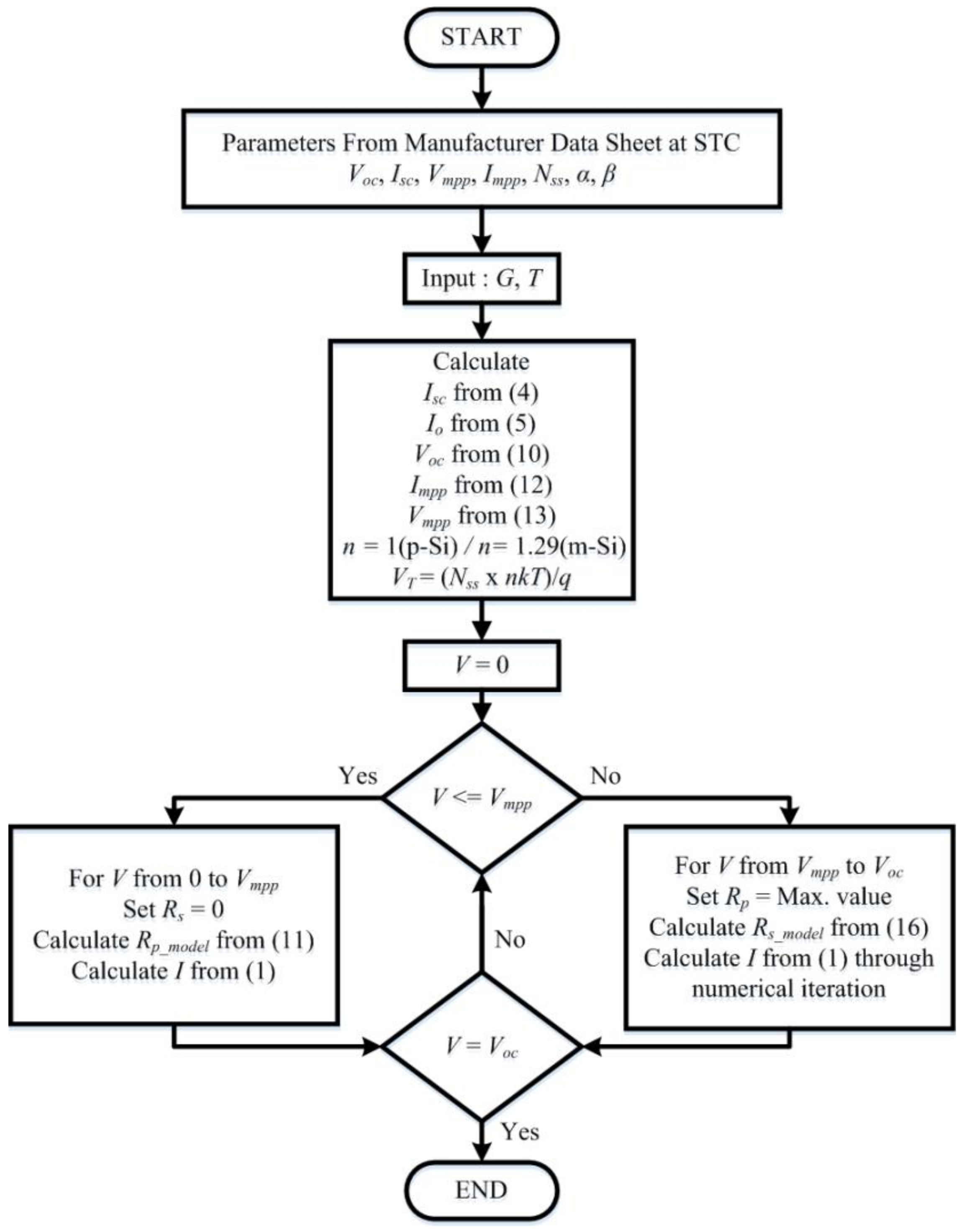
The proposed model can be implemented in software using the flowchart given in Figure 7. Note that from 0 V to MPP point, the proposed model will not use any iterative method to determine either Rp_model or I. However, from MPP to Voc, the model will only utilize simple numerical iteration to calculate I as it appears on both side of Equation (1), while Rs_model is estimated without iteration.
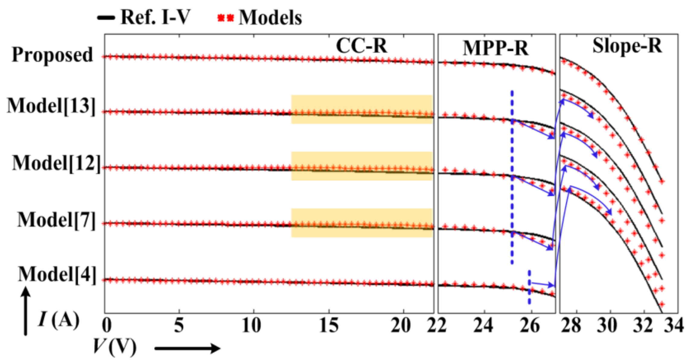
Matlab/Simulink environment is used to simulate the proposed model and numerous recently proposed models [4,7,12,13]. The polycrystalline technology-based PV module of type Kyocera 200GT is selected [24]. The I-V curves of all these models are first generated under STC condition, and comprehensive analysis is carried out. In Figure 8, three windows are highlighted, where in each window black line represents Ref. I-V curve and red dots represent respective performance of model. The Y-axis is a current axis; however, its axis values are irrelevant, as each model is deliberately shifted from other models for better visualization. The first window belongs to the constant current region (CC-R). In this window, the proposed model shows excellent resemblance to Ref. I-V curve and outperforms each model.
The cumulative performance of each model is represented in the form of root mean square error (RMSE) in Table 1. Model [4] also exhibits similar performance, while the remaining models are less accurate in CC-R. The mismatch portions of models [7,12,13] are highlighted in Figure 8.
The window of MPP region is represented next, in which the proposed model perfectly adopts the curvature nature of I-V curve and comprehensively follows the Ref. I-V. Compared to previous region, the RMSE of model [4] is enhanced, whereas other three models become less accurate. A key observation regarding the models [7,12,13] is indicated in Figure 8 that at dotted line position, these models already cross-over the line and start diverging from Ref. I-V curve. This will also produce negative repercussions in the upcoming section, as the arrows show the future trends of these models. Likewise, model [4] does not cross-over the line but struggles to match the knee of curve at the end of MPP-region.
In last Slope (S) region, with the exception of proposed model, the other models do not strictly follow the Ref. I-V. Models [7,12,13] continue to fade away from the Ref. I-V curve, and their curves are situated below the Ref. I-V. Model [4] also shows less accuracy compared to its previous regions, and unlike other models, it stays over the Ref. I-V curve. The proposed model stays close to the Ref. I-V curve.
In Table 1, the accuracy of all models can be sorted in descending order as CC-R, MPP-R, and S-R. The superiority of proposed model can be attributed to three points:
- Its parametric extraction is free from any complex or optimization procedures.
- It provides a non-iterative solution from 0 to Vmpp, while it only requires simple numerical iterations to estimate I from Vmpp to Voc.
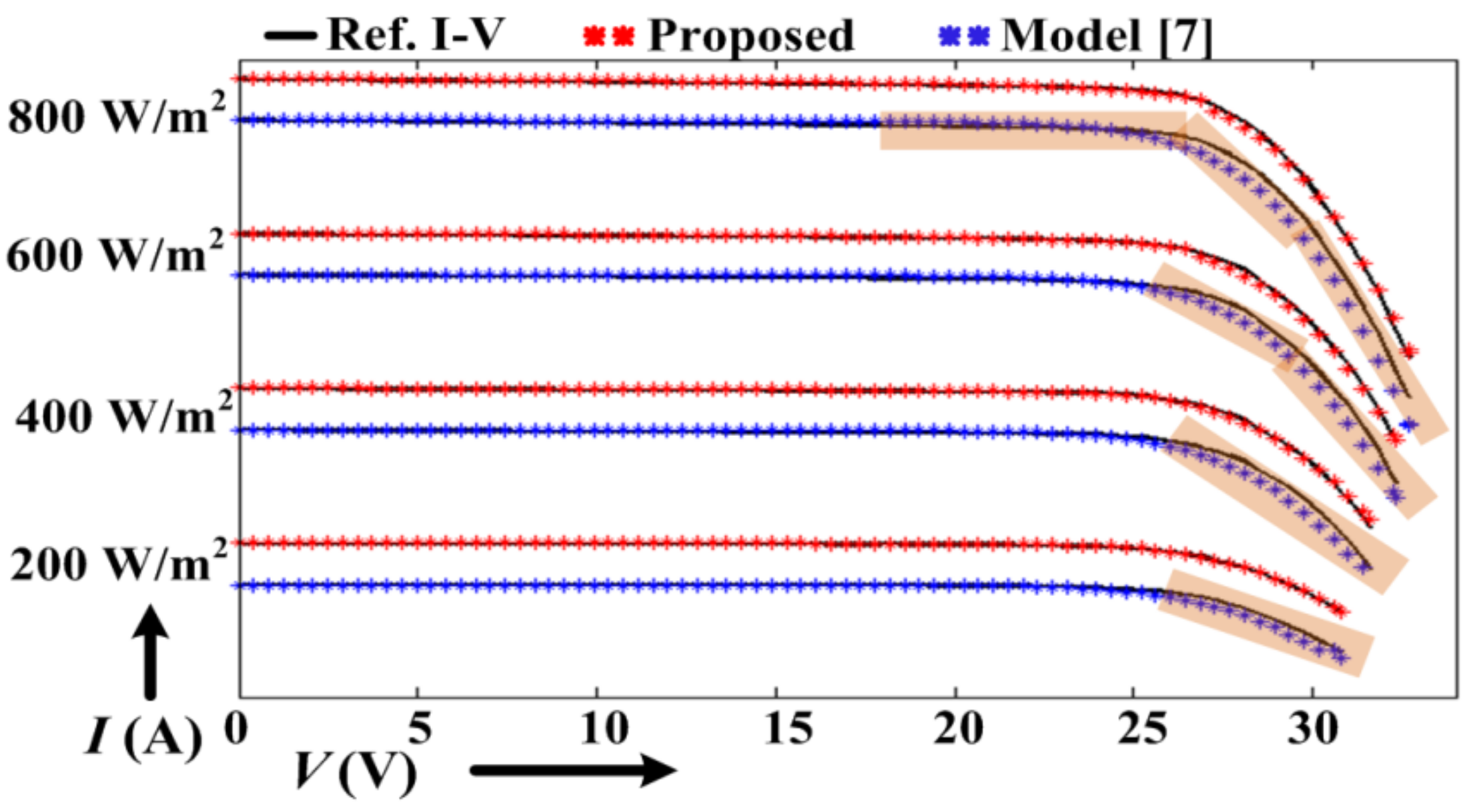
For the remaining conditions, i.e., 800 W/m2, 600 W/m2, 400 W/m2 and 200 W/m2, proposed model is compared with Model [7]. The RMSE values of two models are tabulated in Table 2. In Figure 9, the highlighted portions of different conditions are shown, where model [7] lacks the performance as compared to proposed model. With the exclusion of 200 W/m2, the proposed model holds the one-tenth advantage over model [7]. In addition, the proposed method maintains a similar performance over the entire spectrum of conditions, as depicted by Table 2. The accuracy of model [7] increases with the fall in weather conditions but struggles to produce the accuracy exhibited by proposed method.
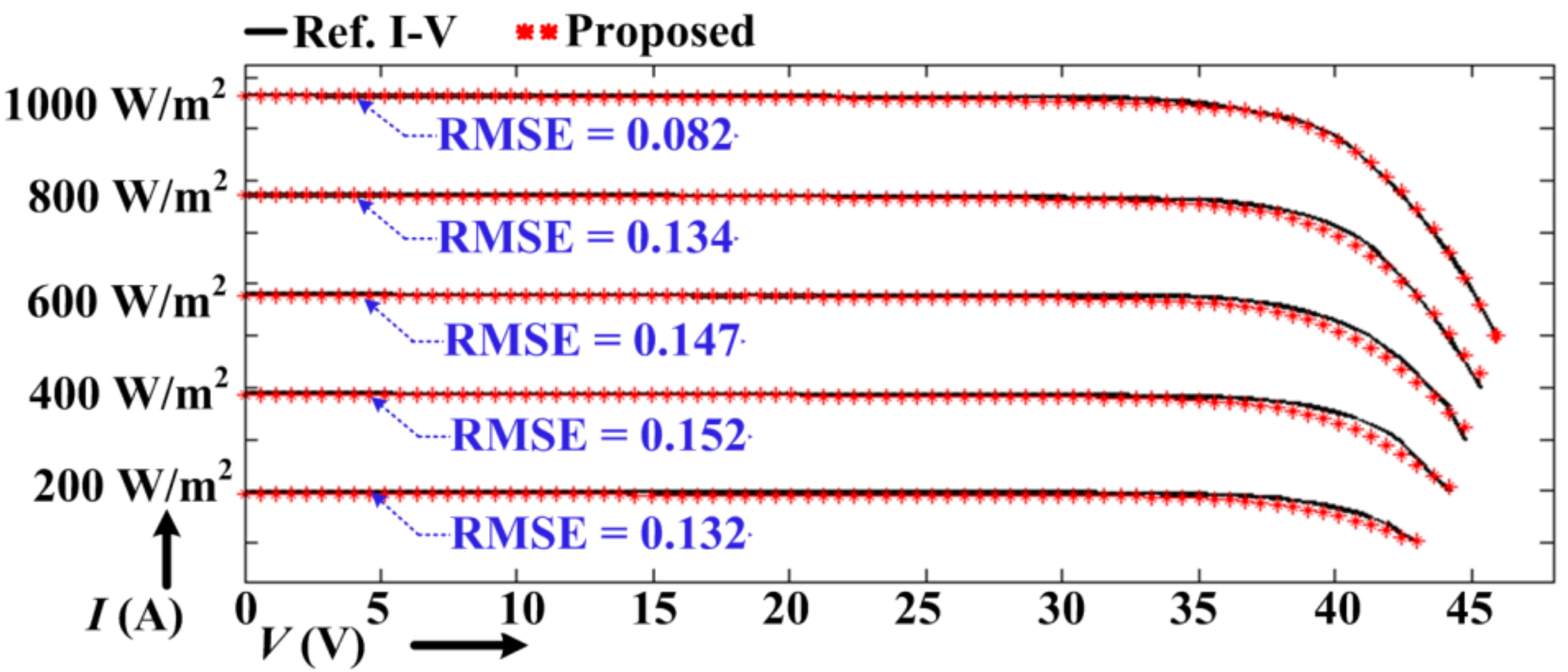
To elaborate, the performance of proposed model, a mono-crystalline (m-Si) PV module SL280-24M330, is selected [25]. The I-V curves of this module are extracted from the datasheet through CAD software in the same fashion as in the previous case. Initially, the model is realized with the same estimations of all parameters as in the case of poly-crystalline (p-Si) PV module [24]. The RMSE errors are high for m-Si module. Afterwards, numerous results are gathered by varying the factor n from 0.5 to 2, and finally the value of n = 1.29 comes out of the optimum value.
The corresponding results are presented in Figure 10, in which five black curves depict the Ref. I-V curves of different irradiance levels. It can be evaluated that the proposed model remains effective and strictly follows the Ref. I-V curve, and the only adjustment is made in n. The RMSE of each weather condition is mentioned in Figure 10 as well. The proposed model can be applicable to any c-Si module without any adjustments in its parameters except n,thus making it a simple and fast model. The optimum values of n are 1 and 1.4 for p-Si technology and m-Si technology, respectively.
As is well established in literature, the temperature change produces major impact in Voc value and minor impact in Isc value [3,4,5,6]. The proposed model has the ability to cope with temperature variations through its Voc and Isc relationships. Expression (10) depicts that the model has the temperature coefficient factor ‘β’ for Voc value. Similarly, (4) has the temperature coefficient factor ‘α’ for Isc value. Through these temperature coefficients, the model updates the values of Voc and Isc for every temperature change. In addition, the effects of temperature variations are also reflected in Vmpp and Impp values. Equations (12) and (13) show that Vmpp and Impp are estimated through Voc and Isc, respectively. In this way, the accuracy of proposed model remains intact with temperature variations.
4. Conclusions
With respect to the usage of the single-diode model with five parameters, its limited accuracy in the simulation of I-V curves is due to two main reasons: (1) the static estimation of the resistive parameters and (2) the fact that only STC data are available in manufacturer’s datasheet. In this paper, the database of I-V curves is developed by using CAD software for crystalline silicon and in the future for thin film technologies. The formulae to estimate resistive parameters are designed through the statistical concept of the weighted mean, MPP parameters, and a large database of I-V curves, the combination of which makes the resistive estimations adaptive for both steady and varying weather conditions, (and it is a non-iterative solution, too). In addition, the same database also provides the facility to compare the I-V curves of different models with the original I-V curves. A comparative analysis reveals superior accuracy, less computation burden, and a low complex algorithm compared to past-proposed models. In terms of root mean square error (RMSE) analysis, the proposed model outscores other models by a one-tenth advantage.
Author Contributions
Conceptualization, A.F.M., U.M., M.C., P.D.L. and F.S.; Formal analysis, A.F.M.; Investigation, A.F.M. and U.M.; Methodology, A.F.M., U.M., M.C., P.D.L. and F.S.; Software, A.F.M. and U.M.; Supervision, F.S.; Validation, M.C., P.D.L. and F.S.; Writing—original draft, A.F.M. and U.M.
Funding
This research received no external funding.
Conflicts of Interest
The authors declare no conflict of interest.
Nomenclature
| I & V | Operating current and voltage of PV module |
| Isc & Voc | Short-circuit current and open-circuit of PV module |
| Impp & Vmpp | Maximum power point current and voltage of PV module |
| Iph | Photo-generated current by the current source |
| ID | Current passing through the diode |
| ki | Proportionality factor between Isc and Impp |
| kv | Proportionality factor between Voc and Vmpp |
| Rs & Rp | Series resistance and parallel resistance of PV module |
| Rs_model | Proposed value of series resistance |
| Rp_model | Proposed value of parallel resistance |
| α | Temperature coefficient of Isc at STC |
| β | Temperature coefficient of Voc at STC |
References
- Cárdenas, A.A.; Carrasco, M.; Mancilla-David, F.; Street, A.; Cárdenas, R. Experimental parameter extraction in the single-diode photovoltaic model via a reduced-space search. IEEE Trans. Ind. Electr. 2017, 64, 1468–1476. [Google Scholar] [CrossRef]
- Sher, H.A.; Murtaza, A.F.; Addoweesh, K.E.; Chiaberge, M. Pakistan’s progress in solar PV based energy generation. Renew. Sustain. Energy Rev. 2015, 47, 213–217. [Google Scholar] [CrossRef]
- Batzelis, E.I.; Papathanassiou, S.A. A Method for the Analytical Extraction of the Single-Diode PV Model Parameters. IEEE Trans. Sustain. Energy 2016, 7, 504–512. [Google Scholar] [CrossRef]
- Silva, E.A.; Bradaschia, F.; Cavalcanti, M.C.; Nascimento, A.J. Parameter estimation method to improve the accuracy of photovoltaic electrical model. IEEE J. Photovolt. 2016, 6, 278–285. [Google Scholar] [CrossRef]
- Hosseini, S.M.H.; Keymanesh, A.A. Design and construction of photovoltaic simulator based on dual-diode model. Sol. Energy 2016, 137, 594–607. [Google Scholar] [CrossRef]
- Ishaque, K.; Salam, Z.; Syafaruddin. A comprehensive MATLAB Simulink PV system simulator with partial shading capability based on two-diode model. Sol. Energy 2011, 85, 2217–2227. [Google Scholar] [CrossRef]
- Hejri, M.; Mokhtari, H. On the Comprehensive Parameterization of the Photovoltaic (PV) Cells and Modules. IEEE J. Photovolt. 2017, 7, 250–258. [Google Scholar] [CrossRef]
- Spertino, F.; D’Angola, A.; Enescu, D.; Di Leo, P.; Fracastoro, G.V.; Zaffina, R. Thermal-electrical model for energy estimation of a water cooled photovoltaic module. Sol. Energy 2016, 133, 119–140. [Google Scholar] [CrossRef]
- Jena, D.; Ramana, V.V. Modeling of photovoltaic system for uniform and non-uniform irradiance: A critical review. Renew. Sustain. Energy Rev. 2015, 52, 400–417. [Google Scholar] [CrossRef]
- Xiao, W.; Edwin, F.F.; Spagnuolo, G.; Jatskevich, J. Efficient approaches for modeling and simulating photovoltaic power systems. IEEE J. Photovolt. 2013, 3, 500–508. [Google Scholar] [CrossRef]
- Rahman, S.A.; Varma, R.K.; Vanderheide, T. Generalised model of a photovoltaic panel. IET Renew. Power Gener. 2014, 8, 217–229. [Google Scholar] [CrossRef]
- Hasanien, H.M. Shuffled Frog Leaping Algorithm for Photovoltaic Model Identification. IEEE Tran. Sustain. Energy 2015, 6, 509–515. [Google Scholar] [CrossRef]
- Moshksar, E.; Ghanbari, T. Adaptive Estimation Approach for Parameter Identification of Photovoltaic Modules. IEEE J. Photovolt. 2017, 7, 614–623. [Google Scholar] [CrossRef]
- Xue, L.; Sun, L.; Wei, H.; Jiang, C. Solar cells parameter extraction using a hybrid genetic algorithm. In Proceedings of the 2011 Third International Conference on Measuring Technology and Mechatronics Automation (ICMTMA), Shanghai, China, 6–7 January 2011. [Google Scholar]
- Huang, W.; Jiang, C.; Xue, L.; Song, D. Extracting solar cell model parameters based on chaos particle swarm algorithm. In Proceedings of the International Conference on Electric Information and Control Engineering, Wuhan, China, 15–17 April 2011. [Google Scholar]
- Veissid, N.; Bonnet, D.; Richter, H. Experimental Investigation of the double exponential of a solar cell under illuminated conditions: considering the instrumental uncertainties in the current, voltage and temperature values. Solid-State Electron. 1995, 38, 1937–1943. [Google Scholar] [CrossRef]
- Cerofolini, G.F.; Polignano, M.L. Generation-recombination phenomena in almost ideal silicon p-n junctions. J. Appl. Phys. 1989, 64, 6349–6356. [Google Scholar] [CrossRef]
- Prorok, M.; Werner, B.; Zdanowicz, T. Applicability of equivalent diode models to modeling various, thin-film photovoltaic (PV) modules in a wide range of temperature and irradiance conditions. Electron Technol. Internet J. 2006, 37, 78–88. [Google Scholar]
- Attivissimo, F.; Adamo, F.; Carullo, A.; Lanzolla, A.M.L.; Spertino, F.; Vallan, A. On the performance of the double-diode model in estimating the maximum power point for different photovoltaic technologies. Measurement 2013, 46, 3549–3559. [Google Scholar] [CrossRef]
- Adamo, F.; Attivissimo, F.; Di Nisio, A.; Spadavecchia, M. Characterization and testing of a tool for photovoltaic panel modeling. IEEE Trans. Instrum. Meas. 2011, 60, 1613–1622. [Google Scholar] [CrossRef]
- Gow, J.A.; Manning, C.D. Development of a photovoltaic array model for use in power-electronics simulation studies. IEE Electr. Power Appl. 1999, 146, 193–200. [Google Scholar] [CrossRef]
- Villalva, M.G.; Gazoli, J.R.; Filho, E.R. Comprehensive approach to modeling and simulation of photovoltaic arrays. IEEE Trans. Power Electr. 2009, 24, 1198–1208. [Google Scholar] [CrossRef]
- Chin, V.J.; Salam, Z.; Ishaque, K. An accurate modelling of the two-diode model of PV module using a hybrid solution based on differential evolution. Energy Convers. Manag. 2016, 124, 42–50. [Google Scholar] [CrossRef]
- Highlights of KYOCERA Photovoltaic Modules. Available online: https://www.kyocerasolar.com/dealers/product-center/archives/spec-sheets/KC200GT.pdf (accessed on 21 May 2018).
- 340 W Maximum Power High Efficiency Mono-crystalline Solar Module. Available online: https://cdn.enfsolar.com/Product/pdf/Crystalline/594749db3bd6f.pdf (accessed on 21 May 2018).
Figure 1.
Basic philosophy of proposed PV model.

Figure 2.
I-V curve of multi-crystalline PV module at distinct irradiance levels [24].
Figure 2.
I-V curve of multi-crystalline PV module at distinct irradiance levels [24].

Figure 3.
Step by step transformation of I-V curves from raw datasheet to useful data, (a) the form of data sheet after conversion into CAD; (b) the appearance of curves after removal of unnecessary information; (c) the scaling of curves as per actual dimensions and measurements; (d) final furnished form of the processed data.

Figure 4.
Ref. I-V curve and I-V curve at Rp_mpp.

Figure 5.
Ref. I-V curves and I-V curves generated at different Rp values.

Figure 6.
Cumulative % error in Rp_Est values.

Figure 7.
Implementation flowchart of the proposed model.

Figure 8.
Resemblance between original I-V curve under STC versus different models’ curves.

Figure 9.
Performance advantage of proposed model over model [7].
Figure 9.
Performance advantage of proposed model over model [7].

Figure 10.
RMSE values of proposed model against I-V curve of different conditions of mono-crystalline module [25].
Figure 10.
RMSE values of proposed model against I-V curve of different conditions of mono-crystalline module [25].


Table 1.
Comparison of RMSE and complexity of different models.
| Models | Root Mean Square Error under STC | Complex/ Optimization Procedures | Iterative Solution | |||
|---|---|---|---|---|---|---|
| Constant Current Region | MPP Region | Slope Region | 0 to Vmpp | Vmpp to Voc | ||
| Proposed | 0.024 | 0.032 | 0.053 | No | No | Yes |
| Model [13] | 0.077 | 0.108 | 0.385 | Yes | Yes | Yes |
| Model [7] | 0.088 | 0.117 | 0.422 | Yes | Yes | Yes |
| Model [12] | 0.069 | 0.111 | 0.441 | Yes | Yes | Yes |
| Model [4] | 0.028 | 0.055 | 0.326 | Yes | Yes | Yes |
Table 2.
RMSE of two models against distinct conditions.
| Conditions at 25 °C | Root Mean Square Error | |
|---|---|---|
| Proposed Model | Model [7] | |
| 800 W/m2 | 0.041 | 0.187 |
| 600 W/m2 | 0.022 | 0.135 |
| 400 W/m2 | 0.031 | 0.115 |
| 200 W/m2 | 0.044 | 0.080 |
© 2018 by the authors. Licensee MDPI, Basel, Switzerland. This article is an open access article distributed under the terms and conditions of the Creative Commons Attribution (CC BY) license (http://creativecommons.org/licenses/by/4.0/).
Share and Cite
MDPI and ACS Style
Murtaza, A.F.; Munir, U.; Chiaberge, M.; Di Leo, P.; Spertino, F. Variable Parameters for a Single Exponential Model of Photovoltaic Modules in Crystalline-Silicon. Energies 2018, 11, 2138. https://doi.org/10.3390/en11082138
AMA Style
Murtaza AF, Munir U, Chiaberge M, Di Leo P, Spertino F. Variable Parameters for a Single Exponential Model of Photovoltaic Modules in Crystalline-Silicon. Energies. 2018; 11(8):2138. https://doi.org/10.3390/en11082138
Chicago/Turabian StyleMurtaza, Ali F., Umer Munir, Marcello Chiaberge, Paolo Di Leo, and Filippo Spertino. 2018. "Variable Parameters for a Single Exponential Model of Photovoltaic Modules in Crystalline-Silicon" Energies 11, no. 8: 2138. https://doi.org/10.3390/en11082138
Note that from the first issue of 2016, this journal uses article numbers instead of page numbers. See further details here.