Multi-Time Scale Rolling Economic Dispatch for Wind/Storage Power System Based on Forecast Error Feature Extraction


1
School of Electrical and Power Engineering, China University of Mining and Technology, Xuzhou 221116, China
2
School of Information and Control Engineering, China University of Mining and Technology, Xuzhou 221116, China
*
Author to whom correspondence should be addressed.
Energies 2018, 11(8), 2124; https://doi.org/10.3390/en11082124
Submission received: 24 July 2018
/
Revised: 4 August 2018
/
Accepted: 7 August 2018
/
Published: 15 August 2018
Abstract
:This paper looks at the ability to cope with the uncertainty of wind power and reduce the impact of wind power forecast error (WPFE) on the operation and dispatch of power system. Therefore, several factors which are related to WPFE will be studied. By statistical analysis of the historical data, an indicator of real-time error based on these factors is obtained to estimate WPFE. Based on the real-time estimation of WPFE, a multi-time scale rolling dispatch model for wind/storage power system is established. In the real-time error compensation section of this model, the previous dispatch plan of thermal power unit is revised according to the estimation of WPFE. As the regulating capacity of thermal power unit within a short time period is limited, the estimation of WPFE is further compensated by using battery energy storage system. This can not only decrease the risk caused by the wind power uncertainty and lessen wind spillage, but also reduce the total cost. Thereby providing a new method to describe and model wind power uncertainty, and providing economic, safe and energy-saving dispatch plan for power system. The analysis in case study verifies the effectiveness of the proposed model.
1. Introduction
In recent years, with the increasing prominence of energy consumption and environmental pollution, renewable energy generation, represented by wind power generation, has been paid more and more attention [1,2]. However, due to the strong uncertain and volatile characteristics of wind power, it is difficult to forecast and model accurately [3,4,5]. Overestimation or underestimation of wind power would lead to reserves under-committed, causing wind curtailment and load shedding [6]. Therefore, how to handle the wind power forecast error (WPFE) becomes a research hotspot [7,8,9].
To cope with the uncertainty of wind power, the dispatch model is mainly divided into two types. The first type is the certain model [10,11,12,13]. For example, in the literature [10], the requirement of spinning reserve and the additional cost caused by the valve point effect are considered. Furthermore, the upward and downward spinning reserve constraints are added to the dispatch model. In Reference [11], the network loss and the spinning reserve requirements for wind power uncertainty are considered, then a multi-objective dispatch model considering both emission and cost is established. This type of model needs to set a large capacity of spinning reserve to ensure the safety of the system operation, which is too conservative and not economical. The second type is the uncertain model, such as probabilistic model [14,15,16,17], fuzzy set theory [18,19], scenario analysis [6,20], stochastic programming theory [21,22,23,24], etc. For example, the authors in Reference [14] regard the forecast error of load demand and wind power as normal distribution, and propose a probabilistic model to estimate the reserve capacity demand. In Reference [19], the authors regard the wind power output as a fuzzy variable and establish a multi-time scale dispatch model considering chance constraints of spinning reserve. In Reference [20], a Monte Carlo sampling method based on polynomial chaotic expansion is proposed and used to generate wind power scenarios. In Reference [23], a risk adjustable unit commitment (UC) optimization model is proposed, which combines the chance constrained programming and the goal programming. Although these sorts of models can describe the uncertainty of wind power in different degrees, they have their own limitations. The choice of the distribution function of the probabilistic model is subjective, and the model is usually complex and time-consuming to solve. The selection of membership function and the fuzzy parameters needs an experience. For the scenario analysis method, a large amount of work is required for scenario generation and reduction. Stochastic programming is often combined with probabilistic model or fuzzy theory, which is also solved subjectively. Additionally, some scholars also handle the uncertainty of wind power using battery energy storage system (BESS) [25,26], electric vehicle (EV) [27,28], or demand side management (DSM) [29,30,31]. For example, in Reference [26], the charge/discharge loss costs of BESS are taken into account, and an optimization dispatch model based on fuzzy set theory is established. In Reference [27], the authors use point estimation method based on Nataf transform to express uncertainties in wind power, and an economic emission dispatch model for power system containing wind farms and EVs is established. As for BESS and DSM, the authors in Reference [29] establish a dynamic economic dispatch model considering the intermittency and uncertainty of power system with high wind penetration. Although the volatility of wind power can be stabilized using these uncertain models, the investment and maintenance cost of BESS is high. Moreover, the uncontrollable EVs and the improper coordination strategy cause more uncertain to power system. In addition, researchers also propose some new methods to describe the uncertainty of wind power. The authors in Reference [32] propose a nonparametric conditional probabilistic forecasting method and present a day-ahead UC model with different wind power forecasting confidence intervals, which can characterize the uncertainty and volatility of wind power. However, the model is also complex, and the selection of leading factors and the partition of space subset are subjective. In Reference [33], the authors propose four kinds of factors, which have positive correlations with WPFE. Based on this, an error estimation model is established by using multiple linear regression method. This model has a certain guiding significance for the estimate of WPFE. However, the actual results fluctuate beyond the estimated range occasionally. Therefore, it is necessary to set up a larger spinning reserve to handle the inaccurate estimate of WPFE.
In this paper, several factors which related to WPFE are analyzed to study how to extract their optimal features through correlation statistics of historical data. Then, according to the optimal factors and correlation coefficients, an estimation indicator for WPFE is calculated. By taking the estimation of WPFE into consideration, a multi-time scale rolling dispatch model based on real-time error compensation is established. The output of thermal power unit (referred to as ‘unit’) is revised based on the estimation of WPFE in real-time error compensation section, and the BESS is utilized to compensate furtherly. The dispatch results and the comparison analysis with alternative models from case study represent the comprehensive performance of proposed method in flexibility, improving wind power accommodation, reducing load shedding, saving computational time and decrease the total cost.
2. WPFE Estimation Based on Optimal Factor Features Extraction
2.1. Analysis on the Method to Extract Probabilistic Optimal Factor Features
In this section, the relationship between several factors and WPFF are analyzed to find the optimal representation of WPFF. WPFF is defined as eW in Equation (1). The factors, including wind power forecast output fluctuation (λ1), short-term wind power output stability (λ2), wind power output amplitude (λ3) and short-term wind power forecast output accuracy (λ4) are listed in Equations (2)–(5). The degree of relationship between these factors and eW is calculated by correlation coefficients, which is defined in Equation (6).
where, subscripts j = {1, 2, 3, 4} represent the four factors respectively. Nj = {N1, N2, N3, N4} are the numbers of sample data used when calculating λj = {λ1, λ2, λ3, λ4}. Rj = {R1, R2, R3, R4} are the correlation coefficients between λj and eW. t is the time label of forecast/dispatch point. wa and wf are the actual and 15 min ahead forecast of wind power. Vcap is the rated capacity of the wind farm.
By using the wind power data gathered from the public database of Elia [34], Rj = {R1, R2, R3, R4} can be calculated. The calculated results indicate that the correlation coefficients Rj are influenced by the numbers of sample data. Too large number of used sample data even leads to a negative Rj. To obtain the optimal factors defined in Equations (2)–(5), the historical wind power data are analyzed to find the optimal number of sample data.
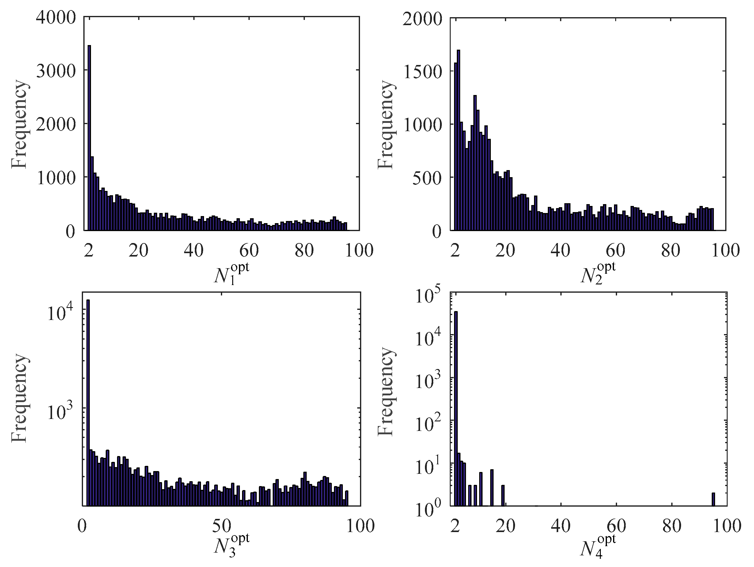
A whole year historical data of wind power is gathered from 1 June 2014 to 31 May 2015 of Elia. The number of used wind data is 365 × 24 × 4 = 35,040. For each time point, λj,t and etW are calculated by using Equations (1)–(5) when Nj = 2~96. After normalization of λj,t and etW, correlation coefficients Rj are calculated through Equation (6). After each step, 95 groups of correlation coefficients are calculated. The largest correlation coefficient Rj and the corresponding number of sample data Nj are obtained. For a whole year data, the previous calculations are implemented for 35,040 times. Then, we can achieve 35,040 groups of largest Rj (Rjopt) and the corresponding optimal Nj (Njopt).
The frequency distribution of Njopt is shown in Figure 1.
In Figure 1, N1opt = 2, the frequency is 3454 accordingly, which is larger than any other values of N1opt. It means that R1 has the largest probability to be optimal when N1opt is 2, namely, λ1 has the strongest relationship to WPFE when N1opt is 2 in Equation (2). For λ2, λ3, λ4, N2opt = 3, N3opt = 2 and N4opt = 2 respectively.
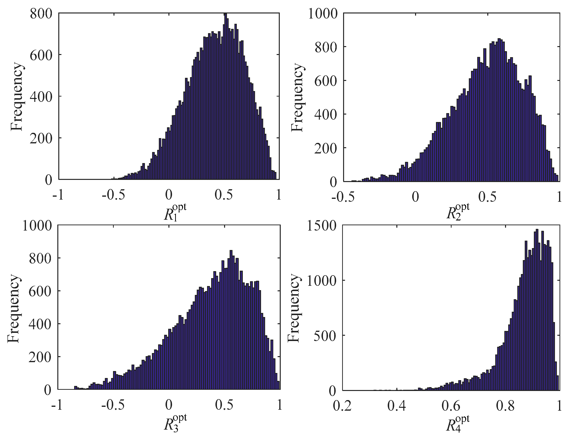
The frequency distribution of Rjopt are also shown in Figure 2.
In Figure 2, the largest frequency is 795 while R1opt ∈ [0.50, 0.52]. It indicates that in 35,040 times of calculation, the times that R1opt ∈ [0.50, 0.52] are 795. The largest frequency is 847 while R2opt ∈ [0.56, 0.58]. The largest frequency is 845 while R3opt ∈ [0.54, 0.56]. The largest frequency is 1460 while R4opt∈ [0.90, 0.92]. The frequency distributions in Figure 2 also indicate that R4opt has the largest probability to large, meaning that λ4 has stronger relationship with WPFE comparing to λ1, λ2, λ3. On the other hand, λ3 has weakest relationship with WPFE. To represent the correlation degree of λ1, λ2, λ3, λ4 with WPFE, the mean of each correlation coefficient Rjopt (Rjmean) are calculated. In Figure 2, R1mean, R2mean, R3mean, R4mean are 0.4152, 0.4932, 0.3778, 0.8716 respectively.
Additionally, the whole year data is divided into four seasons. The optimal values Njopt and the mean of Rjopt of each season and the whole year are listed in Table 1.
In WPFE estimation, the optimal values of different seasons in Table 1 are taken according to different dispatch dates. Among them, Njopt is used to calculate each factor λj to obtain its optimal value λjopt. This process is called optimal factor features extraction, and the normalized λjopt is used to estimate WPFE. Rjmean is used as the weight of each optimal factor λjopt in the estimation process.
The optimal values in this paper are obtained from the statistical analysis results by using the operation data from Elia. When data sets are different, the results may vary. According to the method in this paper, other operation data of wind farms can be statistically calculated to obtain the corresponding optimal values.
2.2. WPFE Estimation Based on Optimal Correlation Weights
From the previous discussion, it can be concluded that λ1, λ2, λ3, λ4 have relationships to WPFE. To estimate the WPFE, an error indicator λe is defined in Equation (7):
where, λe is the weighted average of λ1, λ2, λ3, λ4. By using the mean of correlation coefficient Rjopt as the weights of λ1, λ2, λ3, λ4, different factor influences λe in different degree. λe is more dependent on λ4 because R4mean is larger and λ4 has stronger relationship to forecast error than other three factors λ1, λ2, λ3.
In real time dispatch operation, λjopt and λe can be calculated for each time point based on the most recent data of wind power. By utilizing the historical normalize eW, λe is anti-normalized to obtain the estimation of WPFE (eW). In the dispatch model in next section, λe and eW are used to take the real-time WPFE into consideration.
3. Power System Multi-Time Scale Rolling Dispatch Model Based on Real-time Error Compensation
3.1. The Overall Idea of the Dispatch Model
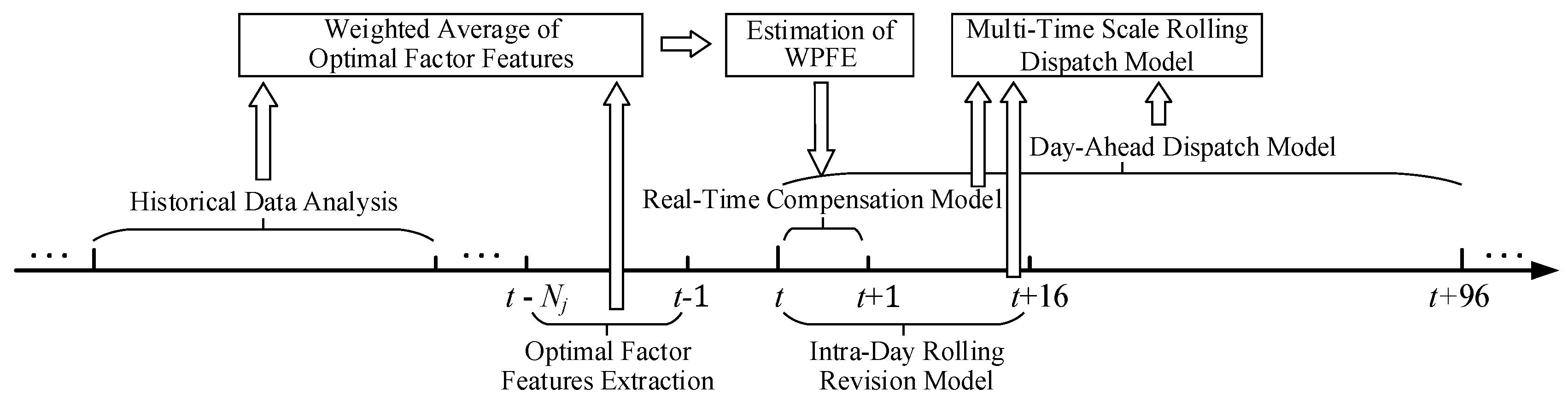
The dispatch model consists of three time-scale parts: (1) Day-ahead dispatch model ([t, t + 96]); (2) intra-day rolling revision model ([t, t + 16]); and (3) real-time error compensation model ([t, t + 1]). UC plan is formulated and adjusted according to the solution of the first two time-scale models. The unit output adjustment plan and charge/discharge plan of BESS are formulated based on the solution of the third time-scale model. Due to the WPFE estimation indicator involved in the third time-scale model, the dispatch schedule can be adjusted following the estimation of WPFE and compensate it on time. In this way, the dispatch schedule can be obtained following the actual wind power as closely as possible, which can keep the balance of power supply and load demand and decrease the wind power curtailment. With the overall ideas above, the time axis flowchart is shown in Figure 3.
In Figure 3, t is the time label of forecast/dispatch point. We analyze the historical data to obtain the optimal value Njopt and Rjmean. Then the recent data ([t − Njopt, t − 1]) is used to extract the optimal factor features λjopt. By the weight of Rjmean, the estimation indictor and the estimation of WPFE are achieved and to be taken into consideration in real-time compensation section of multi-time scale rolling dispatch model.
3.2. Day-Ahead Dispatch Model
The day-ahead dispatch model is established to provide a 24 h plan, ahead of time. It mainly draws up the UC plan, upward and downward spinning reserve for the next day. The goal of this model is to minimize the total cost. Since there are large errors in the day-ahead forecast wind power, some constraints in this model are appropriately relaxed. A larger capacity of spinning reserve would be set up in this step to provide an enough adjustable margin for intra-day rolling revision step.
3.2.1. Objective Functions
Considering the cost of unit coal consumption, start-up, upward and downward spinning reserve, the objective function of the day-ahead dispatch model is presented as follows:
where, the subscripts n and t are unit label and time label. The superscript D-A indicates the parameters in day-ahead model. CP, CS, CU and CD are the cost of unit coal consumption, start-up, upward and downward spinning reserve respectively. N and T are total unit number and total time number. P, rG,u, rG,d are active power output, upward and downward spinning reserve of units respectively. a, b, c are coal consumption cost coefficients of units. s, ku, kd are cost coefficients of unit start-up, upward and downward spinning reserve. uG is start-stop state variable of unit. 1 represents ‘start-up’, while 0 means ‘stop-out’.
3.2.2. Constraints of the Model
1 System Active Power Balance Constraints
where, wf,D−A is the day-ahead forecast of wind power. Lf,D−A is day-ahead forecast of load demand.
2 Unit Output Constraints
where, Pmax and Pmin are the upper limit and lower limit of unit output.
3 Unit Upward and Downward Spinning Reserve Constraints
The spinning reserve upper limits are set considering the maximum available power and the maximum ramping constraint that the unit can provide during dispatch time interval ∆T (15 min). The lower limits of the spinning reserve are set depending on the forecast values, which are expressed as:
where, ru and rd are upper and lower ramping rate of units. kw and kl are reserve capacity demand coefficients of wind farm and load.
3.3. Intra-Day Rolling Revision Model
The intra-day rolling revision model provides a plan which is 15 min to 4 h ahead. This plan is executed based on the results of the day-ahead dispatch decision and the recent ultra-short-term forecast of wind power and load demand. According to the intra-day plan, unit outputs are gradually revised to track the latest forecast values. The UC plans are also tested that whether it is necessary to change the start-stop plan of the unit during the subsequent period.
3.3.1. Objective Functions
Similar to the day-ahead dispatch model, the goal of intra-day rolling revision model is to achieve the minimum total cost. The model is established as follows:
where, the superscript I-D indicates the parameters in intra-day model. ∆P, ∆rG,u and ∆rG,d are revision power of unit output, upward and downward spinning reserve.
3.3.2. Constraints of the Model
1 System Active Power Balance Constraints
where, wf,I−D and Lf,I−D are recent ultra-short-term forecast of wind power and load demand.
2 Unit Output Revision Constraints
Considering the maximum ramp rate and output limits of the unit within the dispatch time interval ∆T, the constraints are listed as follows:
3 Upward and Downward Spinning Reserve Revision Constraint
The spinning reserve upper limits are similar to that in the day-ahead model, which are expressed as:
The spinning reserve lower limits are expressed by chance constraints based on the probabilistic model.
where, eW,p and eL,p are forecast errors of wind power and load demand obtained from the probabilistic models. In the intra-day rolling revision model. it is assumed that eW,p and eL,p all subject to normal distribution, and the parameters can be found in literature [14]. P{·} ≥ α means that the probability of an event is larger than the confidence level α.
Other constraints are similar to the conventional dispatch model.
3.4. Real-Time Error Compensation Model
Real-time error compensation model provides a plan 15 min ahead of time, according to the real-time estimation of WPFE based on the recent data of wind power. Due to the limited capacity and output power of BESS within a short time period, as well as the high operation and maintenance cost of BESS, units are used to prioritize compensation the WPFE within the adjustable range. Then, BESS is used for further compensation. Therefore, the method of block modeling and stratified solution is adopted here. Firstly, the compensation sub-model of unit is established. The total output of units is revised within its adjustable range to compensate the real-time estimation of WPFE. Then, the compensation sub-model of BESS is established. The charge/discharge strategies are formulated to furtherly compensate the estimation of WPFE. Finally, the main model of real-time error compensation is established. By substituting the solutions of the two sub-models into the main model, the total revised output of units is optimized and assigned to each unit with the object of minimizing the total cost.
3.4.1. The Compensation Sub-Model of the Units
In real-time error compensation model, a slack variable et′ is set to ensure that the model has a feasible optimal solution because the estimation of WPFE may not be compensated completely. The slack variable is minimized in the objective function so that the estimation of WPFE can be maximally compensated by the units. The estimation of WPFE etW obtained by the previous method is introduced and the compensation sub-model of the units is established as follows:
where
where the R−T indicates the parameters in real-time model. PR−T is the total output of units after intra-day rolling revision. The decision variable ∆PR−T is the total output of units needs to be revised in this model. PG is the total output of units after revision. ∆Pn′ are revised outputs need to assign to each unit, which are decision variables of the main model. wf and Lf are 15 min ahead forecast of wind power and load demand. The slack variable et′ represents the estimation of WPFE after being compensated by units and is used in the BESS sub-model.
Other constraints are similar to the intra-day model.
3.4.2. The Compensation Sub-Model of BESS
BESS is used to further compensate the estimation of WPFE after being compensated by units. The goal is to maximize the compensated power, meaning that maximize the charge/discharge output of BESS. As a result, the WPFE can be compensated as much as possible. The objective function is established as follows:
where, uB,ch and uB,dc are charge/discharge status variables of BESS (1 for charge/discharge, 0 for pause). PB,ch and PB,dc are the charge/discharge output power of BESS. et′ is used as a compensation demand coefficient to maximize the charge/discharge of BESS.
The BESS sub-model should be satisfied with the following constraints:
1 Charge/Discharge Constraints of BESS
The charge/discharge power of BESS in each dispatch point must be within the maximum and minimum charge/discharge power (PB,max and PB,min) that BESS can provide during the dispatch time interval ∆T:
2 Charge/Discharge Status Constraints of BESS
The charge/discharge consumptions of BESS are taken into consideration. In order to avoid charging and discharging frequently, charge/discharge performs when the magnitude of e′ exceeds a certain threshold.
where
where, RtG,u and RtG,d are the total upward and downward spinning reserve (SR) of units obtained from the chance constraints based on normal distribution model. If the SR is not set properly, it will result in wind curtailment or load shedding. kch and kdc are the charge/discharge threshold coefficient. When kch and kdc are higher (close to 1), the threshold is higher, and the times of charge/discharge is less. As a result, the effect of compensation is likely to reduce due to insufficient ramp rate and output power of BESS during a short time. On the contrary, the smaller kch and kdc are (closer to 0), the more the charge/discharge times and the compensated power are. However, it would increase the frequency of charging and discharging of BESS and the costs. In actual dispatch process, these two parameters can be set according to the compensation requirement.
3 BESS Compensation Range Constraints
The forecast error et′ after being compensated by BESS needs to be within the threshold of units SR:
4 BESS Capacity Constraints
The capacity of BESS after providing charge/discharge power at each time period must be within the BESS available capacity limits.
where, ηB,ch and ηB,dc are charge/discharge efficiency coefficients of BESS. EB, EB,max and EB,min are current available capacity, maximum and minimum available capacity of BESS.
3.4.3. Real-Time Compensation Main Model
The total revision output is assigned to each unit with the object of minimizing the cost. By taking the cost of charge/discharge loss of BESS (CB) into consideration, the main model is established as follows:
where FI−D is the objective function in intra-day model. CI and ntotal are investment cost and life cycles of BESS. Pn,tR−T is the output of unit n in dispatching time t after intra-day rolling revision. The decision variable ∆Pn,t′ is the revision output needs to distribute to unit n in dispatching time t. PtG is the total output of units in dispatching time t after revision by unit compensation sub-model.
Other constraints are similar to the intra-day model.
3.5. The Transformation and Solving Method for the Model
The multi-time scale rolling dispatch model established in this paper is a mixed integer nonlinear programming (MINLP) problem with chance constraints including uncertainty variables. Because of the large number of decision variables, the linear programming commercial solving software CPLEX is used in this paper. The first is to transformer the dispatch model to a linear and deterministic one.
3.5.1. Piecewise Linearization of Coal Consumption Cost
In this paper, the coal consumption cost CP in objective functions Equations (9) and (15) are nonlinear. The method in literature [26] is used to divide the cost curve of coal consumption into three equal parts to convert the nonlinear quadratic function to a linear piecewise function.
3.5.2. Simplification of Chance Constraints
In this paper, the chance constraint Equation (19) is nonlinear and containing uncertain variables. We use the method in literature [24] to make a deterministic and linear transformation for chance constraints. The forecast errors eW,p and eL,p are treated as normal distribution. Then the Fast Fourier Transform (FFT) is used to quickly calculate the convolution of them to obtain the probability density function of joint variable Zt. Next, according to the correspondence table in Reference [24], the cumulative distribution function of joint variables (FZt) is obtained. Finally, the dichotomy method is used to obtain the inverse function of Cumulative Distribution Function (CDF, FZt−1). Under the confidence levels αu and αd, the deterministic constraints are obtained as follows.
After the above deterministic and linearization processing, the model transforms to a MILP problem. Then CPLEX is used to solve the model, which can save a lot of calculation time.
3.5.3. The Overall Flowchart of the Proposed Method and Model
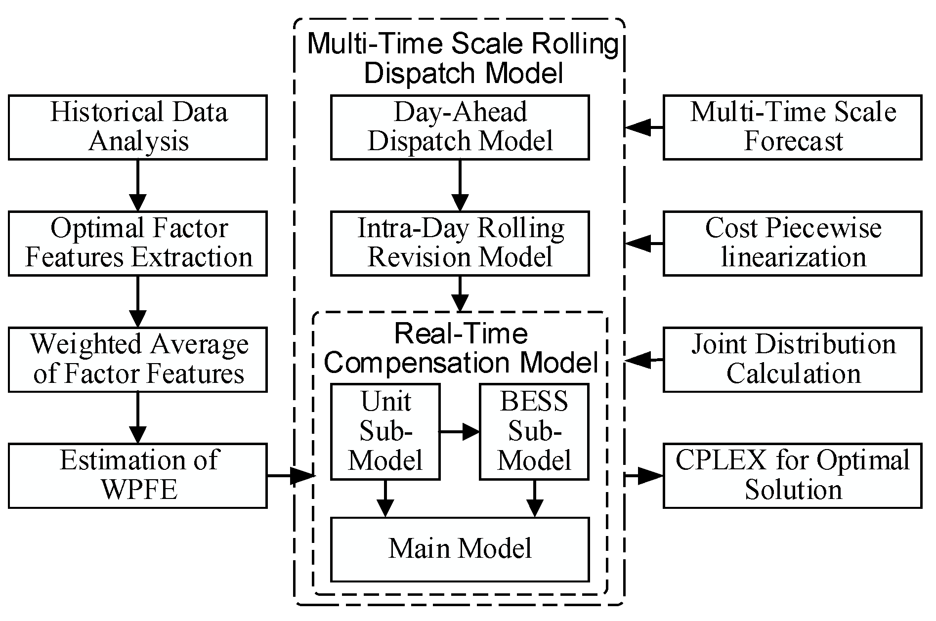
Integrating the estimation method, dispatch model and solution method proposed above, the flowchart is shown in Figure 4.
As shown in the middle part of Figure 4, the day-ahead dispatch model and the intra-day rolling revision model of multi-time scale rolling dispatch model is solved successively according to the forecast wind power at the corresponding time scale. Then, in the left part of Figure 4, WPFE is estimated by historical data analysis, optimal factor features extraction and weighted average of factor features. Finally, the real-time compensation model is solved to adjust units and BESS in real time based on the result of the intra-day rolling revision model and the estimate WPFE. In the whole solution process, the piecewise of coal consumption cost and the joint distribution calculation of wind power and load demand is adopted to linearize the model for optimal solution by using CPLEX.
4. Case Study
4.1. Case Analysis
The IEEE 39-bus test system and IEEE 118-bus test system are used respectively to illustrate the effectiveness of the dispatch model in WPFE compensation, four cases are set as follows:
- Case 1: The dispatch model consists of day-ahead dispatch model and intra-day rolling revision model. According to the chance constraint based on probability distribution of intra-day model, the spinning reserve (SR) are set to provide compensation. Real-time compensation section is not taken into consideration.
- Case 2: The dispatch model consists of day-ahead dispatch model, intra-day rolling revision model, real-time compensation sub-model of units and real-time compensation main model. Real-time estimation of WPFE is compensated only by the units.
- Case 3: The dispatch model consists of day-ahead dispatch model, intra-day rolling revision model, real-time compensation sub-model of BESS and real-time compensation main model. Real-time estimation of WPFE is compensated only by the BESS.
- Case 4: The dispatch model consists of day-ahead dispatch model, intra-day rolling revision model, real-time compensation sub-model of unit, real-time compensation sub-model of BESS and real-time compensation main model. Real-time estimation of WPFE is compensated by the units and the BESS.
All experiments are solved using the commercial software CPLEX12.8 MILP solver with MATLAB 2016a and are run on a computer with Intel Core 2.6 GHz CPU and 4G RAM.
4.2. Simulation and Analysis in IEEE 39-Bus System
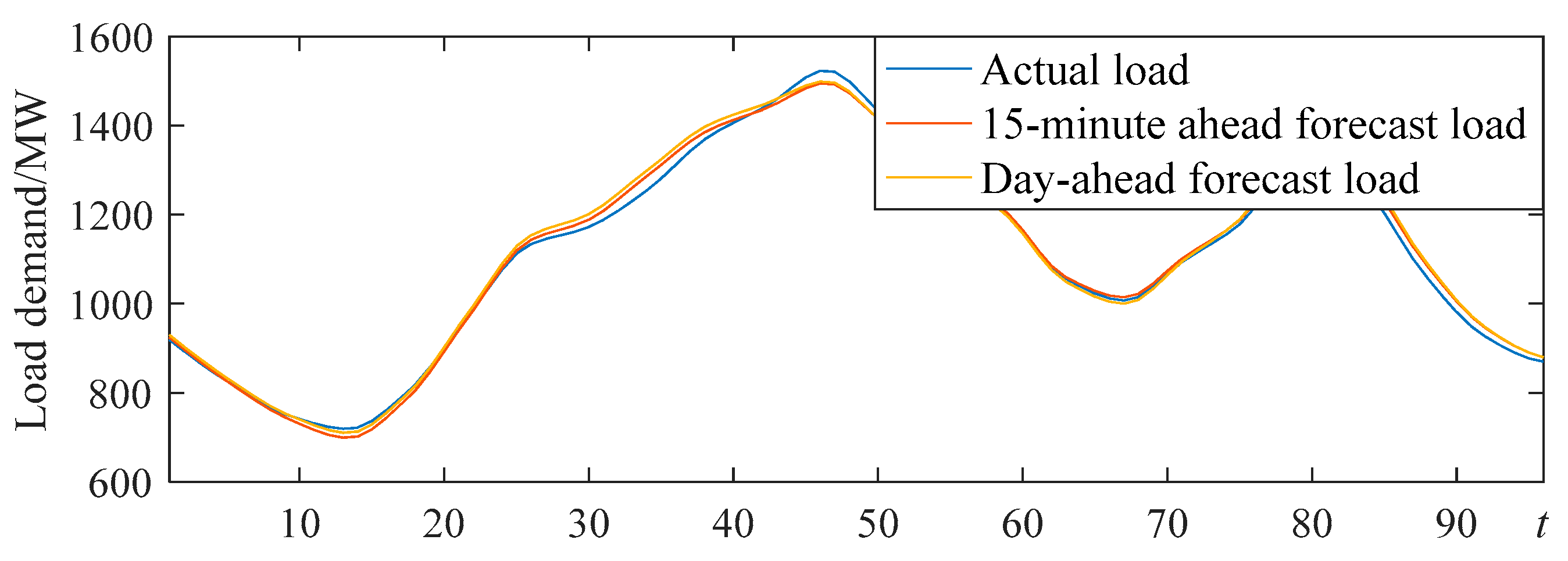
The data in March 2017 from the Elia company is used to test. The wind power data are normalized with rated capacity of 350 MW. The wind/storage system is connected to the 10-unit system. The parameters of the units can be found in literature [35]. The actual and forecast load demand is shown in Appendix A, Figure A1. The values of parameters in the model are shown in Table 2.
4.2.1. Estimation of Wind Power Forecast Error
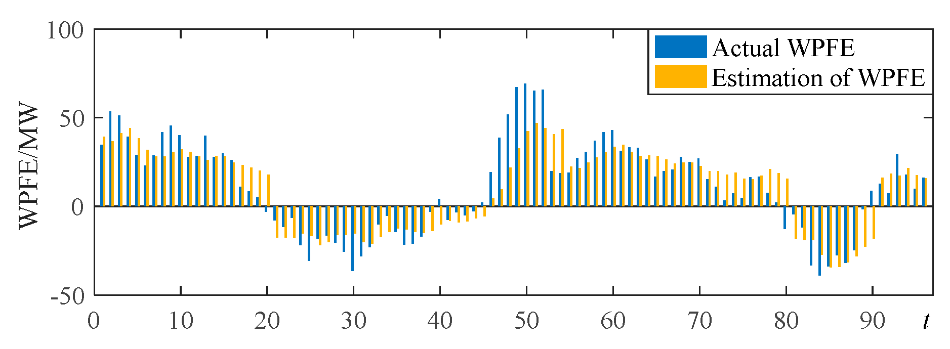
According to the spring optimal Njopt in Table 1, the factors are calculated using Equations (2)–(5) and normalized to obtain λ1,topt,n~λ4,topt,n. Then, according to the spring optimal Rjopt in Table 1, the WPFE estimation indicator λte is calculated by using Equation (7). The indicator λte is then anti-normalized to obtain the estimation of WPFE. The actual WPFE and the estimation of WPFE are shown in Figure 5. The wind power data used in Figure 5 is on 29 March gathered from Elia.
It can be seen that the actual WPFE can be estimated to different degrees in each sample time. When t = 85, the estimation of WPFE obtained by using this method is −34.04MW, and the actual WPFE is −34.48MW. The actual WPFE at the 85th sample time has been estimated accurately. When t = 50, the estimation of WPFE is 42.23 MW, and the actual WPFE is 69.22 MW. Although there is a large gap between the estimation of WPFE and the actual one, the WPFE is evaluated to be a large one and will be compensated in the proposed real-time error compensation model. Otherwise, without the estimation of WPFE (even is not precise enough), the system would face an unbalance of 69.22 MW instead of 26.99 MW (69.22 − 42.23 = 26.99).
In this paper, the real-time compensation model considering the WPFE estimation indicator is established on the basis of the units’ SR based on the chance constraint of probabilistic model in the intra-day dispatch model. By adjustment by units or BESS in advance, the actual invested SR of units can be reduced, so that more adjustable space of SR can be remained to cope with the sudden forecast error peak. The system operating risk including wind power curtailment and load shedding can be reduced.
In addition, the correlation coefficients between λ1opt~λ4opt and WPFE are expressed as R1~R4, and the correlation coefficient between λe and WPFE is represented as Re. They are calculated and shown in Table 3.
From Table 3, it can be seen that the correlation between a single factor and WPFE is relatively low. The largest correlation coefficient among the four factors is 0.5336 and the minimum is only 0.0831. However, the correlation coefficient of the indicator λe obtained by the comprehensive factor features reaches to 0.8775. Therefore, the WPFE can be estimated more accurately by λe.
4.2.2. Analysis of Case 1
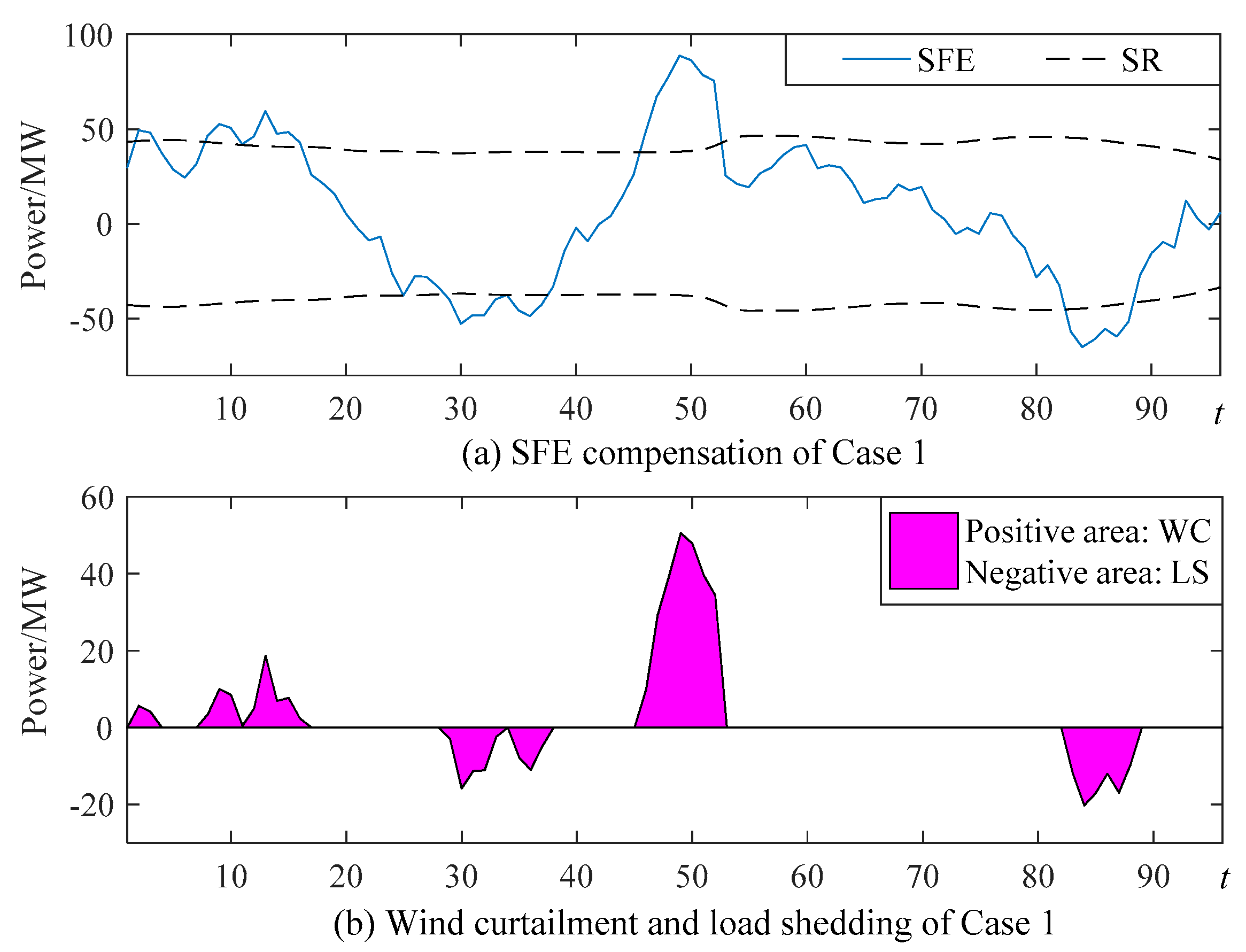
This case is a traditional multi-time scale rolling economic dispatch model based on chance constraint for power system containing a wind farm. After intra-day rolling revision, the grid dispatch schedule tracks to the 15 min ahead forecast of wind power. With the confidence levels αu = αd = 0.9 are set, the chance constraint model, based on normal distribution, are solved to get the possible range of WPFE. The upward and downward SR of units are set accordingly, which are the dotted line in Figure 6a. The Synthetic Forecast Error (SFE) is the sum of the actual forecast error of wind power and load demand, as shown by the blue line in Figure 6a. When the SFE is within the two dotted lines, it can be compensated completely by the SR. Otherwise, incomplete compensation of the SFE results in wind power curtailment (WC, represented as the positive area) and load shedding (LS, represented as the negative area), as shown in the purple area in Figure 6b.
For t = 50 in Figure 6a, the actual WPFE is 69.22 MW and the load forecast error is −17.14 MW. It is an extreme situation while wind power is underestimated, and the load demand is overestimated at the same time. The SFE reaches to 86.36 MW and exceeds the SR = −38.43 MW. In Figure 6b, the wind power curtailment is 47.93 MW at t = 50, and the ratio of the wind power curtailment is 16.7%. For t = 85 in Figure 6a, the actual WPFE is −34.48 MW, and the load forecast error is 26.69 MW. The extreme situation of wind power overestimation and load demand underestimation is occurred. The SFE reaches to −61.17 MW, which greatly exceeds SR = 44.09 MW. At this time, the load demand of −17.08 MW had to be removed and the load shedding ratio was 1.2% as shown in in Figure 6b.
In 96 sample times, the times that SFE exceeds the SR range reach to 34. The total invested SR is 623.1 MW, the total wind power curtailment is 324 MW and the total load shedding is 155.6 MW. It is difficult to compensate the sudden peaks of forecast error by the SR according to the chance constraint based on probabilistic model, thus resulting in larger wind power curtailment and load shedding.
4.2.3. Analysis of Case 2
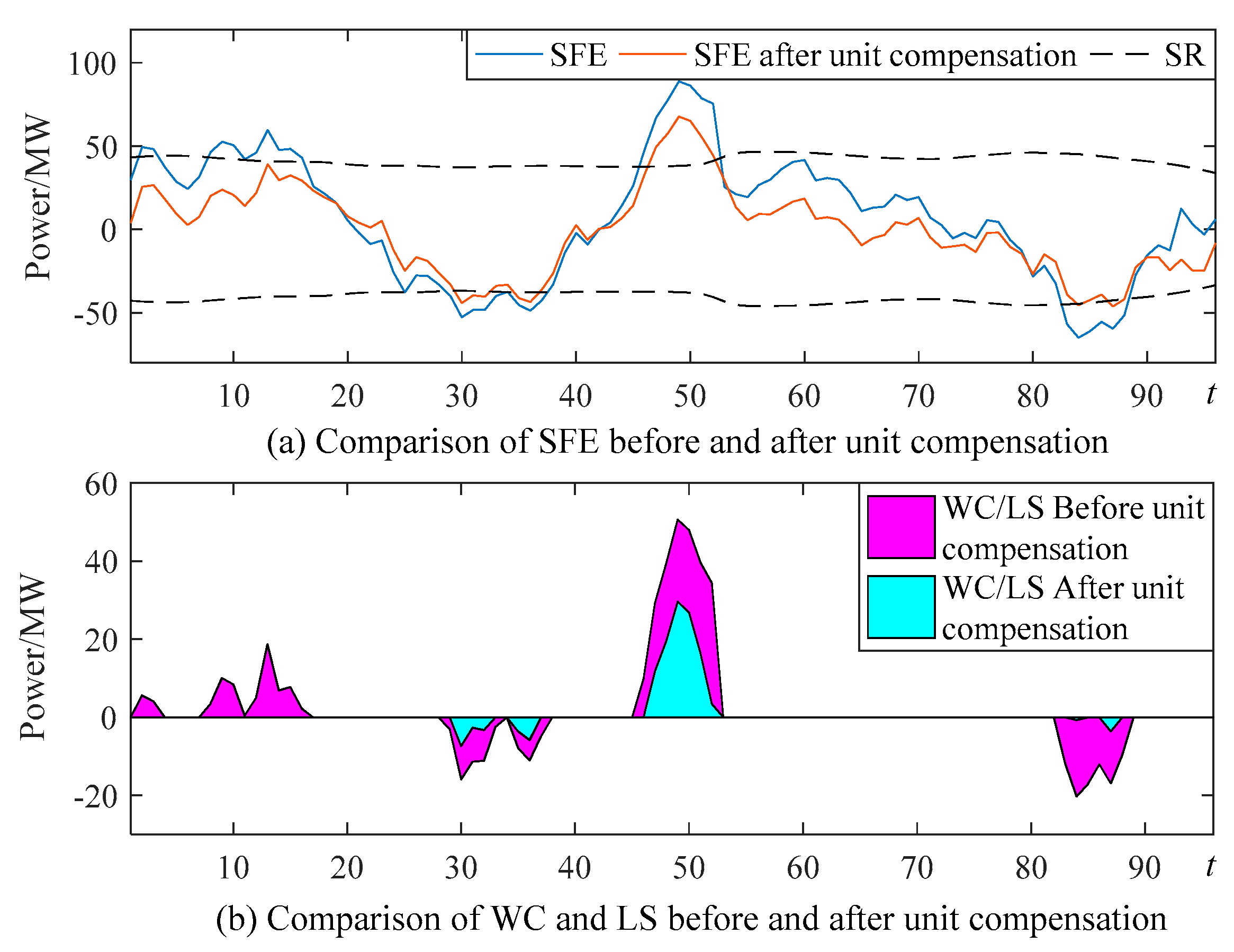
According to the estimation of WPFE, the real-time compensation section is taken into consideration. In Case 2, only the units are responsible for real-time compensation task. The SFE before and after compensation of units are shown in Figure 7a. The wind power curtailment (WC, represented as the positive area) and load shedding (LS, represented as the negative area) before and after compensation of units are shown in Figure 7b.
It can be seen from Figure 7a that depending on the real-time compensation sub-model of units, the SFE is compensated to a great extent. For t = 50, compared with Case 1, the SFE is decreased from 86.36 MW to 65.21 MW, with a reduction rate of 24.5%. As shown in Figure 7b, the wind power curtailment at this time is reduced from 47.93 MW to 26.78 MW, with a reduction rate of 44.1%. For t = 85 in Figure 7a, the SFE is decreased from −61.17MW to −44.09MW after being compensated by units, with a reduction rate of 27.9%. At this time, the load shedding in Figure 7b is decreased from −17.08 MW to 0 MW.
Among the 96 sample times, compared with Case 1, the times that SFE exceed the SR range decreases from 34 to 14. The invested SR of units decreases from 623.1 MW to 466.3 MW, with a reduction rate of 25.2%. The total wind power curtailment decreases from 324 MW to 107.6 MW, with a reduction rate of 66.8%. The total load shedding decreases from 155.6 MW to 27.2 MW, with a reduction rate of 82.5%.
Thus, due to the advanced compensation, the invested SR of units can be reduced. So that the SR has more adjustable space to cope with the sudden peak of forecast error and reduce the wind curtailment and load shedding. However, due to the constraints such as unit ramp rate, the compensation capacity that the units can provide in a short time period is limited. Therefore, the wind curtailment and load shedding is not compensated completely only by units.
4.2.4. Analysis of Case 3
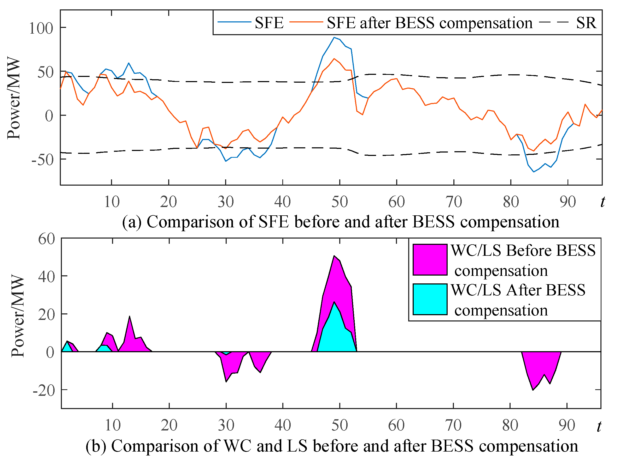
In this case, only the BESS is used to compensate the SFE. The SFE before and after compensation by BESS are shown in Figure 8a. The wind power curtailment (WC, represented as the positive area) and load shedding (LS, represented as the negative area) before and after compensation by BESS are shown in Figure 8b.
The compensation effect on the SFE is also acceptable by using charge/discharge of BESS based on the estimation of WPFE. For t = 50 in Figure 8a, after being compensated by BESS, the SFE decreases from 86.36 MW (in Case 1) to 59.64 MW, with a reduction rate of 30.9%. At this time, the wind power curtailment in Figure 8b decreases from 47.93 MW to 21.21 MW, with a reduction rate of 55.7%. For t = 85 in Figure 8a, after being compensated by BESS, the SFE decreases from −61.17 MW to −44.09 MW, with a reduction rate of 27.9%. At this time, the load shedding in Figure 8b is decreased from −17.08 MW to 0 MW.
Among the 96 sample times, compared with Case 1, the times that SFE exceed the SR range decreases from 34 to 10. The invested SR of units decreases from 623.1 MW to 518.6 MW, with a reduction rate of 16.8%. The total wind power curtailment decreases from 324 MW to 112.8 MW, with a reduction rate of 65.2%. The total load shedding decreases from 155.6 MW to 1.6 MW, with a reduction rate of 99.0%.
The charge/discharge power and the states of charge (SOC) of the BESS in each sample time are shown in Figure 9.
In the model proposed in this paper, compensation is only performed when the estimation of WPFE is greater than a certain threshold (kch/kdc × SR). Refer to Equation (23) for details. In this paper, kch = kdc = 0.8. As can be seen from Figure 9, the BESS schedule has 43 charge and discharge times at 96 sample times. The charge/discharge times are relatively concentrated. Too frequent charge and discharge do not occur. The upper and lower limits of the available capacity of the BESS are indicated by the dotted lines in Figure 9. It can be seen that the BESS schedule satisfies the available capacity constraints at each sample time. As the BESS has a limited charge/discharge power and ramp rate in a short time period, the SFE cannot be completely compensated only by the BESS.
4.2.5. Analysis of Case 4
From the results of Case 2 and Case 3, it can be seen that due to the ramp rate of units and the charge/discharge capacity constraints of BESS, only the unit or only the BESS has a deviation in compensating the SFE. Therefore, the multi-time-scale rolling dispatch model of power system based on real-time error compensation established in this paper integrates these two methods into the real-time compensation section. The effects on power system dispatch after compensation by units and BESS are analyzed in this case. According to the real-time error compensation model in 2.3, the units are adjusted firstly to compensate the estimation of WPFE, and then the charge/discharge of BESS are used to compensate further. The SFE before and after compensation by units and BESS are shown in Figure 10a. The wind power curtailment (WC, represented as the positive area) and load shedding (LS, represented as the negative area) before and after compensation by units and BESS are shown in Figure 10b.
From Figure 10, it can be seen that the compensation method in this case has the best compensation effect on SFE among the four cases. For t = 50 in Figure 10a, after being compensated by units and BESS, the SFE decreases from 86.36 MW to 42.28 MW, with a reduction rate of 51.0%. At the same time, the wind power curtailment in Figure 10b decreases from 47.93 MW to 3.85 MW, with a reduction rate of 92.0%. For t = 85 in Figure 10a, after compensation in this case, the SFE decreases from −61.17 MW to −17.32 MW, with a reduction rate of 71.7%. At this time, the load shedding in Figure 10b decreases from −17.08 MW to 0 MW, and it can be completely avoided.
In the 96 sample times, the times that the SFE exceed the SR decreases from 34 to 4. The invested SR decreases from 623.1 MW to 353.5 MW, with a reduction rate of 43.3%. The total wind power curtailment decreases from 324.0 MW to 32.4 MW, with a reduction rate of 90.0%. The total load shedding decreases from 155.6 MW to 0, with a reduction rate of 100.0%.
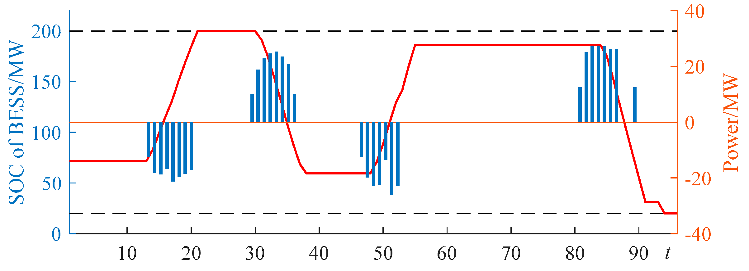
The charge/discharge power and the SOC of the BESS in each sample time are shown in Figure 11.
As can be seen from Figure 11, in the 96 sample times of Case 4, the charge and discharge times of BESS decreases from 43 to 32 compared with being compensated only by BESS in Case 3, which reduces the charge and discharge loss of BESS. The charge/discharge times are very concentrated, and the frequent charge and discharge implements do not occur. From the SOC curve in Figure 11, the BESS schedule satisfies the available capacity constraints in each sample time.
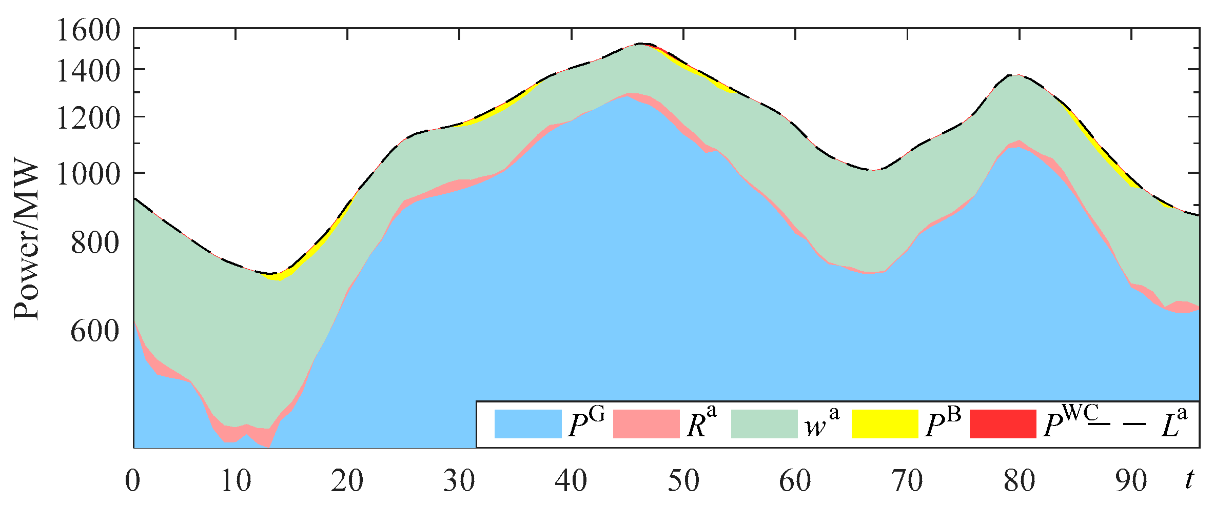
The total output of units (PG), the total invested upward and downward SR of units (Ra, which includes Ru,a and Rd,a), the actual wind power (wa), the charge/discharge power of BESS (PB, which includes PB,ch and PB,dc), wind curtailment and load shedding (PWC and PLS), the total power supply and the load demand (Ptotal and La) in each sample time of this case are shown in Appendix A, Table A1. The power balances in each sample time are verified by area stack diagram, as shown in Figure 12.
The results in Appendix A, Table A1 and Figure 12 indicate that for the 96 sample times in one day, except for the SFE at t = 47~50, which is too large to be fully compensated, the SFE at other sample times can be compensated completely. Therefore, the wind power curtailment and load shedding in most sample times can be eliminated. This shows that the method is effective, and the model is reasonable.
4.2.6. Comprehensive Comparison of Cases
The operation costs in all sample times of Cases 1−4 are shown in Table 4.
In Table 4, CP and CS are costs of unit coal consumption and start-up. CU and CD are costs of invested unit upward and downward SR. CB is charge/discharge loss costs of BESS. Ctotal is the total cost. CR is operation risk penalty cost, which includes wind power curtailment penalty cost (CWC) and load shedding penalty cost (CLS). The cost penalty coefficients are set as $25/MW and $18.75/MW respectively.
From the comparison of power generation costs in Table 4, the costs of the invested SR decrease to a large extent by advanced adjustments in Case 2 and Case 3. In Case 2, the cost of the invested SR decreases from $10,604.50 to $8274.00, which has a reduction rate of 22.0% compared with Case 1. In Case 3, the cost of the invested SR decreases from $10,604.50 to $8740.30, which has a reduction rate of 17.6% compared with Case 1. Furtherly, the cost of invested SR in Case 4 decreases from $10,604.50 to $6234.50, which has a reduction rate of 41.2% compared with Case 1. At the same time, due to the priority adjustment of the unit, the charge and discharge times of BESS in Case 4 are significantly reduced compared with Case 3. Thereby, the charge/discharge loss cost of BESS is decreased from $1655.50 to $1232.00, with a reduction rate of 25.6%.
From the comparison of system operation risk penalty cost in Table 4, it can be seen that the unit SR set based on the probability distribution model (Case 1) can hardly cope with large forecast errors during actual operation, the system operation risk penalty costs are high. Based on the WPFE estimation method in this paper, with the advanced adjustment of Case 2, the operation risk penalty cost decreases from $11,017.50 to $3200.00, with a reduction rate of 71.0% compared with Case 1. Similarly, with the advanced adjustment of Case 3, the operation risk penalty cost decreases from $11,017.50 to $2850.00, with a reduction rate of 74.1% compared with Case 1. Furtherly, after compensation by units and BESS in Case 4, the operation risk penalty cost decreases from $11,017.50 to $810.00, with a reduction rate of 92.6% compared with Case 1. At the same time, the total costs in Case 4 can be minimum, which has a reduction of $16,574.90 compared with Case 1.
The computational times to solve Case 1 to Case 4 are listed in Table 5.
It can be seen from Table 4 and Table 5 that Case 1 has a shortest computational time but with the largest wind curtailment, load shedding and total cost. Conversely, Case 4 can achieve the best dispatch result than Case 2 and Case 3 without sacrificing a lot of computing times. Therefore, it is worthwhile to spend more little time to get the best results.
4.2.7. Analysis for Different BESS Capacities
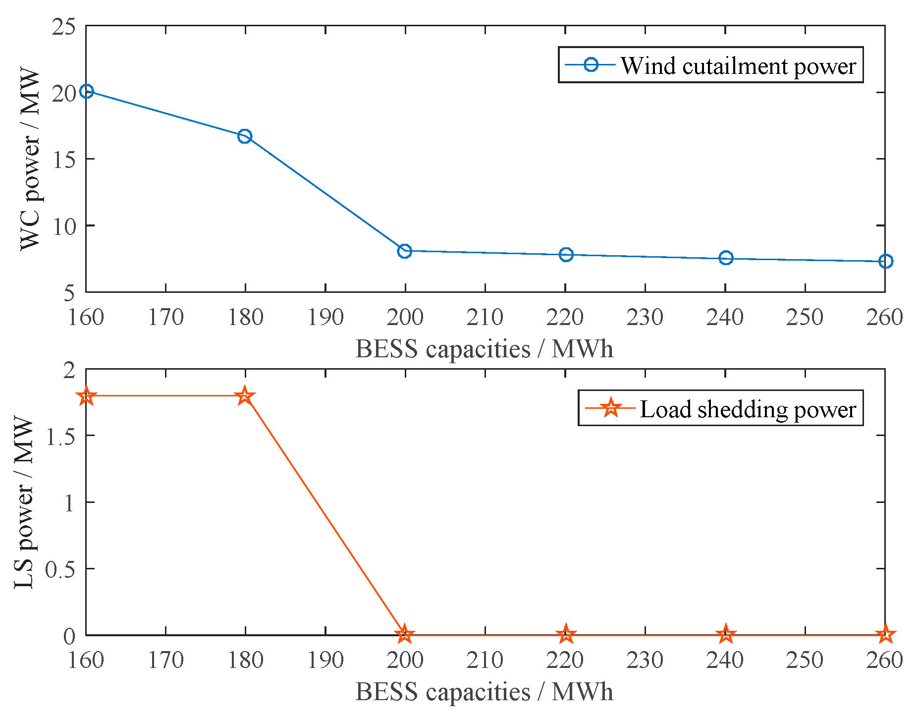
Further, in order to reflect the improvement to the dispatch results by the different BESS capacities, the capacities of BESS are changed with the step of 10 MW. The wind curtailment and load shedding power in different BESS capacities are shown in Figure 13.
It can be seen from Figure 13 that with the increase of BESS capacity, both the wind curtailment and load shedding show a decreasing trend. By comparing the decreasing trend, it can be found that when the BESS capacity is larger than 200 MW, the increase of the BESS capacity is not obvious for the improvement of the wind curtailment and load shedding. The reason is not the insufficient of BESS capacity, but that the BESS can charge or discharge a limited power in a short period of time. Therefore, the improvement for wind curtailment and load shedding is not obvious but the cost of BESS is increased when the BESS capacity is too large. Therefore, it is necessary to properly allocate the BESS capacity and the discussion in this section may be helpful. Reasonable adjustment of the charge/discharge threshold coefficient of BESS described in Equation (23) can extend the adjustment time of BESS, so that it can be adjusted in advance to achieve the goal of no wind curtailment. This is specifically analyzed in Section 4.3.3.
4.3. Simulation and Analysis in IEEE 118-Bus System
To further illustrate the effectiveness of the proposed method and model and its optimization effect in large-scale power systems, the IEEE 118-bus system consists of 186 transmission lines, 54 thermal power units, 91 load points and 3 connected wind farms are used to test. The data in March 2017 from Elia company is used to test. The wind power data are normalized with rated capacity of 600 MW. The parameters of the units can be found in literature [36]. The values of parameters in the model are shown in Table 6.
4.3.1. The Estimation of WPFE
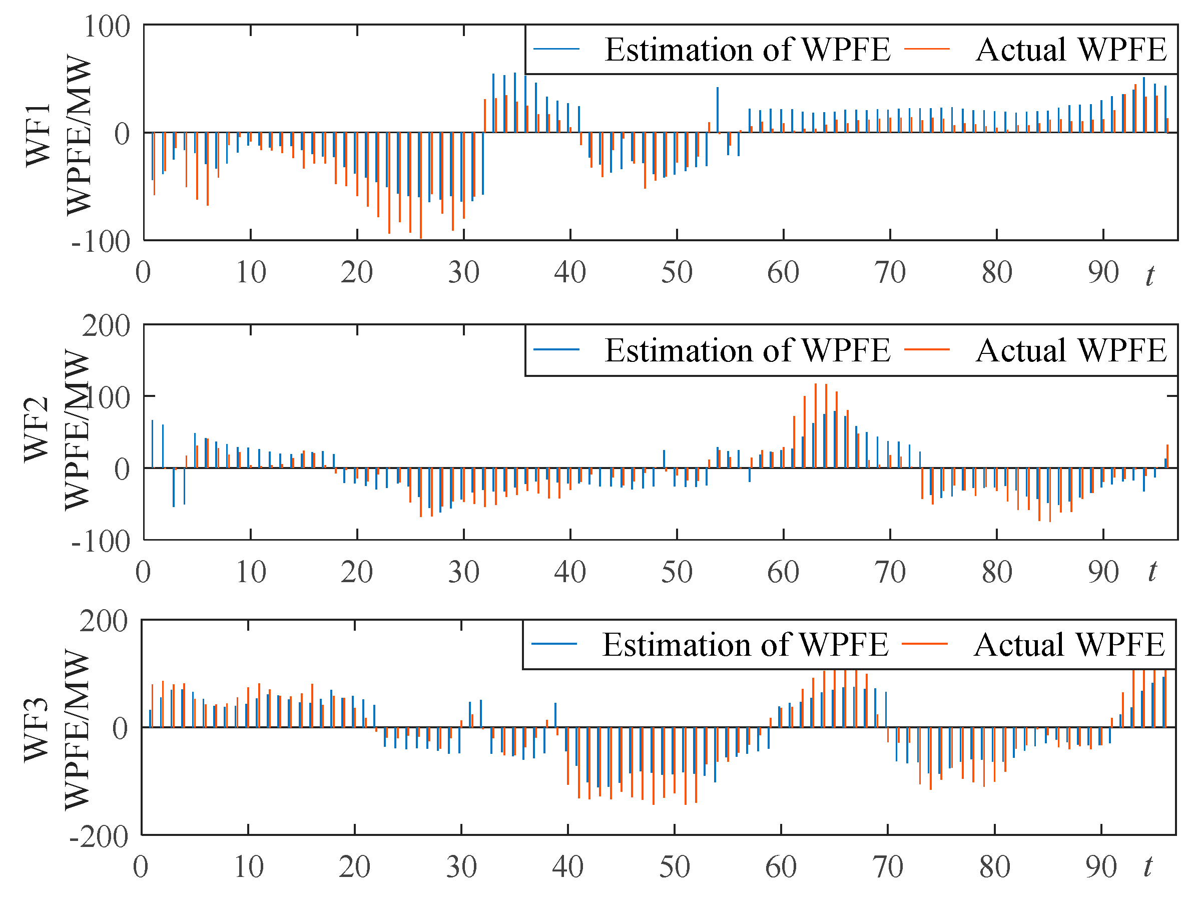
The wind power data in 2 to 4 March 2017 from Elia company are used respectively for the three wind farms (WF1, WF2, WF3). The WPFE of them is estimated according to the previous method. The comparison between the actual and the estimation of WPFE are shown in Figure 14.
It can be seen from Figure 14 that the trend and magnitude of the estimation and the actual WPFE of the three wind farms are approximately the same trend. The correlation coefficients between them are 0.8587, 0.7942, and 0.8949 respectively. It shows that the WPFEs are well estimated.
4.3.2. Analysis of Dispatch Results of Case 4
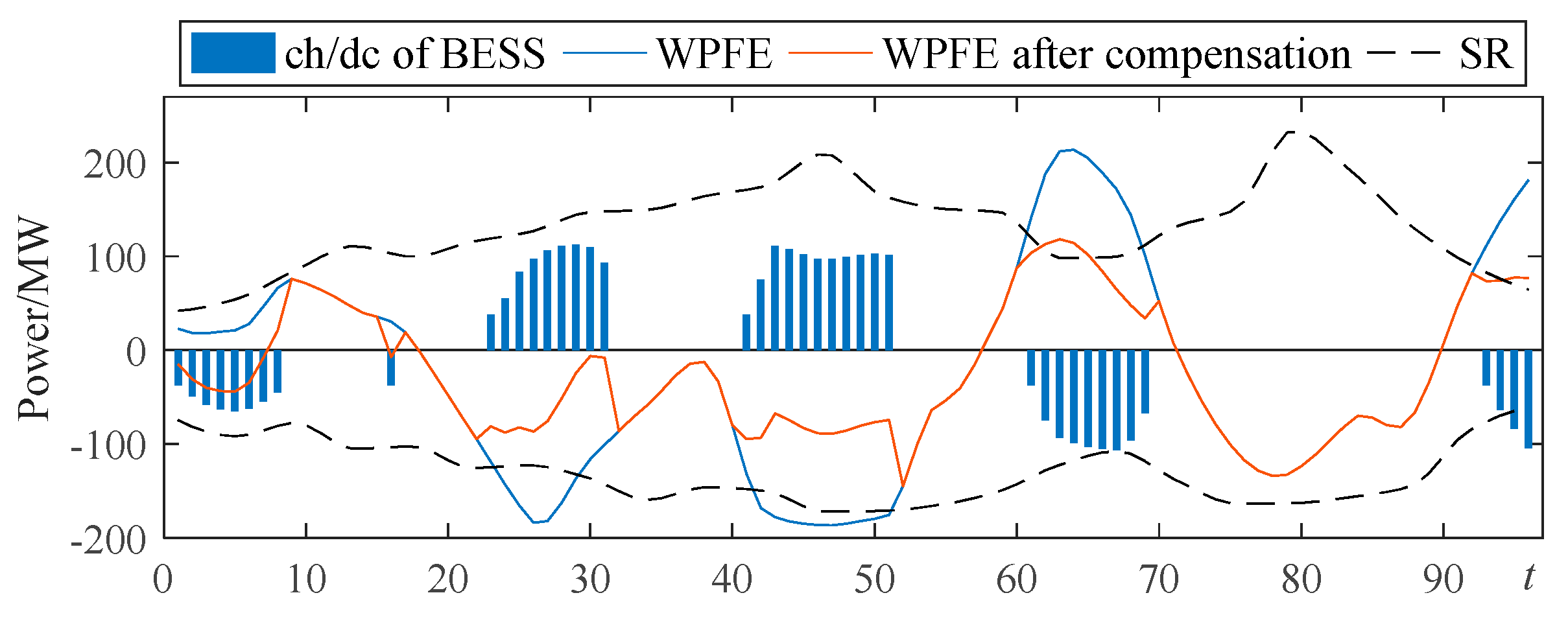
According to the estimation of WPFE, the multi-time scale rolling dispatch model is optimized with the settings of Case 4. The results before and after the compensation by units and BESS are obtained, as shown in Figure 15.
In Figure 15, SR is the upward and downward spinning reserve that all start-up units can provide in a single time period (15 min). The WPFE (the blue curve) is compensated to the red curve by unit and BESS. The blue histogram shows the charge and discharge power of BESS (positive values for discharge and negative values for charge). It can be seen from the blue curve in Figure 15 that before compensation by units and BESS, the WPFE exceeds the boundary of SR multiple times. In the whole dispatch period, 941.5 MW of wind curtailment and 372.4 MW of load shedding power are caused. The wind curtailment rate reaches to 3.7%, and the system operation risk is high. After compensation by units and BESS, the WPFE is well stabilized to the adjustable range of SR for most of sample times. In 96 sample times, except for a small amount of wind curtailment near t = 63 and t = 96, there is no wind curtailment in other sample times. The wind curtailment is 67.9 MW, which is reduced by 873.6 MW than before compensation. The wind curtailment rate is reduced to 0.28%. No load shedding occurs in all sample times.
4.3.3. Analysis for Different Charge/Discharge Threshold of BESS
According to the Equation (23) and its description, the setting of different charge and discharge thresholds of BESS (kch and kdc) have an effect on the dispatch results such as the number of charge and discharge times, the cost of BESS, the amount of wind curtailment and load shedding. The relationship between them are shown in Table 7.
It can be seen from Table 7 that with the decrease of charge/discharge thresholds, the times of charge and discharge times of BESS increase accordingly. The WPFE can be well compensated, and the amount of wind curtailment and load shedding are also reduced. At the same time, the cost of BESS increases accordingly. When the thresholds decrease to 0.8, the load shedding reduces to 0 MW, and a small amount of wind is curtailed. When the thresholds reduce to 0.7, the WPFE can be fully compensated. At this time, the wind curtailment and load shedding reduce to 0 MW, but the charge and discharge times of BESS also increase to 46 and the cost also reaches to the highest. Therefore, this threshold can be adjusted for requirement in actual dispatch process.
4.3.4. Analysis and Comparison with Alternative Models
The various dispatch costs of Case 4 proposed in this paper for IEEE 118-bus test system are shown in Table 8.
Where, CP and CS are costs of unit coal consumption and start-up. CSR are costs of invested unit upward and downward SR. CB is charge/discharge loss costs of BESS. CWC and CLS are penalty costs of wind power curtailment and load shedding. Ctotal is the total cost.
The results of the proposed multi-time scale dispatch model (M-T SDM) in this paper and the results of several models in the literature [36] for the IEEE 118-bus test system are compared in terms of total cost, calculation time and wind curtailment rate, as shown in Table 9.
It can be seen from Table 9 that in the control of wind curtailment, the fully adaptive two-stage robust UC model proposed in Reference [36] and the multi-time scale rolling dispatch model based on real-time error adjustment proposed in this paper can achieve both satisfactory results. The wind curtailment rates of these models are mostly controlled below 1%. By reasonably setting up the wind power scenarios and the establish of unified robust-stochastic model, the method in Reference [36] can achieve a lower wind curtailment rate than the stochastic model and the robust model. However, with a large number of variables and constraints, especially the increase of scenarios, the computational time of the unified robust-stochastic model is still too long, although the author is trying to shorten it. Compared with this, there are fewer variables and constraints of the multi-time scale dispatch model proposed in this paper, which can significantly save computational time with almost the same amount of the wind power accommodation. Thus, it saves precious time for the system adjustment. In addition, the expression of wind power by any method or model will inevitably cause errors, and it is difficult to cope with large error fluctuations only by units. Therefore, the model in this paper can reduce wind power curtailment to a greater extent by adjusting the charge and discharge threshold of BESS, and in this case, the wind curtailment rate can be reduced to 0%. Of course, this is a trade-off between the wind curtailment and the investment of BESS. It is worth noting that due to the differences in the settings of the established models and parameters, the calculation results of the total cost are different, but the overall gap is not large.
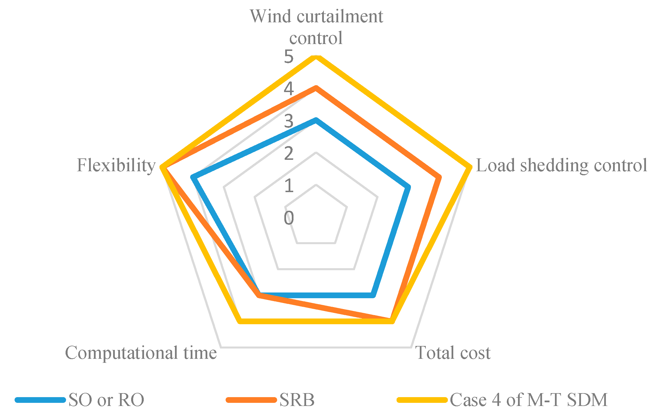
After the above analysis, we comprehensively evaluate the stochastic (SO), robust (RO), unified robust–stochastic (SRB) and the multi-time scale dispatch model (M-T SDM).
Figure 16 shows the strengths of the five abilities of these models from inside to outside. It is divided into five levels, and the larger the number is, the stronger the abilities are. For flexibility, wind curtailment control and load shedding control, by the adjustment of objective function weight, level of conservation and wind curtailment penalty coefficient, the SRB model can balance the wind curtailment rate and the total cost flexibility. However, it is constrained by the large wind power expression errors and the adjustable range of the units and cannot completely eliminate the wind curtailment or load shedding. On the contrary, the M-T SDM in this paper can achieve the trade-off between wind curtailment, load shedding and the investment of BESS by the adjustment of charge/discharge threshold and the cost coefficient of BESS. It can also completely compensate the WPFE and reduce the wind curtailment and load shedding to 0. Therefore, the SRB and the M-T SDM have the same level in flexibility, and the M-T SDM have the higher level in wind curtailment control and load shedding control than SRB. For computational time and total cost, as described above, the M-T SDM with fewer variables and constraints spend much less time to solve than SRB model. The total cost of them are almost the same. Therefore, the SRB and the M-T SDM have the same level in total cost, and the M-T SDM have the higher level in computational time. Finally, as illustrated in Figure 16, the comprehensive level among five abilities of M-T SDM is higher than SRB model.
5. Conclusions and Discussion
This paper proposes a WPFE estimation method based on optimal factor features extraction. A multi-time rolling dispatch model for wind/storage power system based on real-time WPFE estimation is established. The results of case analysis illustrate:
- According to wind power forecast output fluctuation, short-term wind power output stability, wind power output amplitude and short-term wind power forecast output accuracy, a weighted average indicator is obtained to estimate the WPFE. The estimation of WPFE can measure the actual WPFE accurately.
- The estimation of WPFE obtained by this method is introduced, and a multi-time scale rolling dispatch model based on day-ahead dispatch model, intra-day rolling revision model and real-time error compensation model is established. The model can arrange the compensation plan of units and BESS in real-time, thereby increase the adjustable space of the SR set by probability model.
- The case study of 10-units power system with wind farms, and BESS, verifies that the WPFE estimation method and dispatch model proposed in this paper are reasonable and effective. The obtained dispatch plan can maximally track the actual wind power, minimize the wind curtailment and load shedding. Therefore, the security and economic results can be obtained.
Although the work of this paper has achieved economic, security and energy-saving dispatch method as much as possible, the indescribability of wind power brings inevitable errors to the dispatch work. More accurate results may be obtained by finding and analyzing factors that are more correlated with wind power forecast errors. In addition, the current model is slightly complicated and spent long time to solve. How to build a more concise and effective model to save computing time while maintaining performance is also a research point. Moreover, how to take more accurate and effective methods to forecast and model wind power will be the focus of the author's next research.
Author Contributions
All of the authors have contributed to this research. L.H. and X.W. provide the research ideas and guide the revision of the draft; R.Z. and Y.D. perform case studies, analysis, write and revised the paper.
Funding
This research was funded by [the Fundamental Research Funds for the Central Universities] grant number [2017XKQY032].
Acknowledgments
This work is supported by the Fundamental Research Funds for the Central Universities 2017XKQY032.
Conflicts of Interest
The authors declare no conflict of interest.
Appendix A
Figure A1.
The actual and forecast load demand.


Table A1.
The operation of system dispatch plan in each time period.
| Time | PG/MW | Ru,a/MW | Rd,a/MW | wa/MW | PB,ch/MW | PB,dc/MW | PWC/MW | PLS/MW | Ptotal/MW | La/MW |
|---|---|---|---|---|---|---|---|---|---|---|
| 1 | 620.7 | 0.0 | −3.9 | 302.6 | 0.0 | 0.0 | 0.0 | 0.0 | 919.4 | 919.4 |
| 2 | 595.3 | 0.0 | −25.6 | 324.1 | 0.0 | 0.0 | 0.0 | 0.0 | 893.9 | 893.9 |
| 3 | 571.5 | 0.0 | −26.5 | 324.6 | 0.0 | 0.0 | 0.0 | 0.0 | 869.6 | 869.6 |
| 4 | 549.5 | 0.0 | −18.1 | 315.4 | 0.0 | 0.0 | 0.0 | 0.0 | 846.8 | 846.8 |
| 5 | 529.5 | 0.0 | −9.4 | 305.4 | 0.0 | 0.0 | 0.0 | 0.0 | 825.5 | 825.5 |
| 6 | 510.5 | 0.0 | −2.7 | 297.1 | 0.0 | 0.0 | 0.0 | 0.0 | 804.9 | 804.9 |
| 7 | 491.7 | 0.0 | −7.5 | 300.4 | 0.0 | 0.0 | 0.0 | 0.0 | 784.5 | 784.5 |
| 8 | 475.2 | 0.0 | −20.2 | 311.2 | 0.0 | 0.0 | 0.0 | 0.0 | 766.2 | 766.2 |
| 9 | 463.3 | 0.0 | −23.9 | 312.5 | 0.0 | 0.0 | 0.0 | 0.0 | 751.8 | 751.8 |
| 10 | 457.2 | 0.0 | −20.6 | 304.6 | 0.0 | 0.0 | 0.0 | 0.0 | 741.2 | 741.2 |
| 11 | 455.6 | 0.0 | −14.1 | 289.8 | 0.0 | 0.0 | 0.0 | 0.0 | 731.3 | 731.3 |
| 12 | 457.4 | 0.0 | −22.0 | 288.1 | 0.0 | 0.0 | 0.0 | 0.0 | 723.5 | 723.5 |
| 13 | 461.4 | 0.0 | −26.6 | 296.9 | −12.5 | 0.0 | 0.0 | 0.0 | 719.2 | 719.2 |
| 14 | 469.1 | 0.0 | −11.5 | 282.2 | −18.1 | 0.0 | 0.0 | 0.0 | 721.7 | 721.7 |
| 15 | 488.2 | 0.0 | −13.8 | 281.2 | −18.7 | 0.0 | 0.0 | 0.0 | 737.0 | 737.0 |
| 16 | 515.7 | 0.0 | −12.5 | 274.6 | −16.8 | 0.0 | 0.0 | 0.0 | 761.1 | 761.1 |
| 17 | 547.4 | 0.0 | −1.9 | 265.0 | −21.3 | 0.0 | 0.0 | 0.0 | 789.2 | 789.2 |
| 18 | 581.0 | 0.5 | 0.0 | 256.6 | −19.6 | 0.0 | 0.0 | 0.0 | 818.5 | 818.5 |
| 19 | 625.2 | 2.6 | 0.0 | 247.5 | −18.4 | 0.0 | 0.0 | 0.0 | 856.8 | 856.8 |
| 20 | 675.5 | 9.4 | 0.0 | 233.5 | −17.2 | 0.0 | 0.0 | 0.0 | 901.2 | 901.2 |
| 21 | 724.9 | 0.0 | −4.0 | 225.4 | 0.0 | 0.0 | 0.0 | 0.0 | 946.3 | 946.3 |
| 22 | 767.6 | 0.0 | −1.1 | 221.3 | 0.0 | 0.0 | 0.0 | 0.0 | 987.8 | 987.8 |
| 23 | 811.6 | 0.0 | −5.2 | 226.0 | 0.0 | 0.0 | 0.0 | 0.0 | 1032.4 | 1032.4 |
| 24 | 854.4 | 12.3 | 0.0 | 209.9 | 0.0 | 0.0 | 0.0 | 0.0 | 1076.5 | 1076.5 |
| 25 | 889.1 | 24.7 | 0.0 | 198.9 | 0.0 | 0.0 | 0.0 | 0.0 | 1112.7 | 1112.7 |
| 26 | 909.4 | 16.7 | 0.0 | 207.9 | 0.0 | 0.0 | 0.0 | 0.0 | 1134.0 | 1134.0 |
| 27 | 920.7 | 18.9 | 0.0 | 205.8 | 0.0 | 0.0 | 0.0 | 0.0 | 1145.3 | 1145.3 |
| 28 | 929.0 | 26.2 | 0.0 | 198.2 | 0.0 | 0.0 | 0.0 | 0.0 | 1153.3 | 1153.3 |
| 29 | 936.7 | 33.0 | 0.0 | 191.6 | 0.0 | 0.0 | 0.0 | 0.0 | 1161.3 | 1161.3 |
| 30 | 946.1 | 34.1 | 0.0 | 182.1 | 0.0 | 10.0 | 0.0 | 0.0 | 1172.4 | 1172.4 |
| 31 | 957.4 | 20.7 | 0.0 | 191.5 | 0.0 | 18.9 | 0.0 | 0.0 | 1188.4 | 1188.4 |
| 32 | 970.2 | 17.5 | 0.0 | 197.7 | 0.0 | 22.9 | 0.0 | 0.0 | 1208.3 | 1208.3 |
| 33 | 986.0 | 9.2 | 0.0 | 210.9 | 0.0 | 24.6 | 0.0 | 0.0 | 1230.7 | 1230.7 |
| 34 | 1006.3 | 7.9 | 0.0 | 214.8 | 0.0 | 25.3 | 0.0 | 0.0 | 1254.3 | 1254.3 |
| 35 | 1035.0 | 17.8 | 0.0 | 204.9 | 0.0 | 23.4 | 0.0 | 0.0 | 1281.1 | 1281.1 |
| 36 | 1071.5 | 22.5 | 0.0 | 196.9 | 0.0 | 20.9 | 0.0 | 0.0 | 1311.8 | 1311.8 |
| 37 | 1109.6 | 26.1 | 0.0 | 196.8 | 0.0 | 10.1 | 0.0 | 0.0 | 1342.5 | 1342.5 |
| 38 | 1142.8 | 26.4 | 0.0 | 199.9 | 0.0 | 0.0 | 0.0 | 0.0 | 1369.0 | 1369.0 |
| 39 | 1167.9 | 8.2 | 0.0 | 213.1 | 0.0 | 0.0 | 0.0 | 0.0 | 1389.3 | 1389.3 |
| 40 | 1189.4 | 0.0 | −2.6 | 219.6 | 0.0 | 0.0 | 0.0 | 0.0 | 1406.4 | 1406.4 |
| 41 | 1209.5 | 6.2 | 0.0 | 206.6 | 0.0 | 0.0 | 0.0 | 0.0 | 1422.2 | 1422.2 |
| 42 | 1230.4 | 0.0 | −0.3 | 208.6 | 0.0 | 0.0 | 0.0 | 0.0 | 1438.8 | 1438.8 |
| 43 | 1255.5 | 0.0 | −1.4 | 205.0 | 0.0 | 0.0 | 0.0 | 0.0 | 1459.1 | 1459.1 |
| 44 | 1285.7 | 0.0 | −6.6 | 205.4 | 0.0 | 0.0 | 0.0 | 0.0 | 1484.5 | 1484.5 |
| 45 | 1312.8 | 0.0 | −14.3 | 209.7 | 0.0 | 0.0 | 0.0 | 0.0 | 1508.2 | 1508.2 |
| 46 | 1328.0 | 0.0 | −32.9 | 227.8 | 0.0 | 0.0 | 0.0 | 0.0 | 1522.9 | 1522.9 |
| 47 | 1322.4 | 0.0 | −37.7 | 248.0 | 0.0 | 0.0 | −11.8 | 0.0 | 1520.8 | 1520.8 |
| 48 | 1294.6 | 0.0 | −37.9 | 262.1 | −12.5 | 0.0 | −7.1 | 0.0 | 1499.3 | 1499.3 |
| 49 | 1254.1 | 0.0 | −38.1 | 280.3 | −19.8 | 0.0 | −9.8 | 0.0 | 1466.7 | 1466.7 |
| 50 | 1210.5 | 0.0 | −38.4 | 286.9 | −22.9 | 0.0 | −3.8 | 0.0 | 1432.2 | 1432.2 |
| 51 | 1171.8 | 0.0 | −33.1 | 287.4 | −22.3 | 0.0 | 0.0 | 0.0 | 1403.7 | 1403.7 |
| 52 | 1128.4 | 0.0 | −30.8 | 292.5 | −13.6 | 0.0 | 0.0 | 0.0 | 1376.5 | 1376.5 |
| 53 | 1082.5 | 0.0 | −3.3 | 296.0 | −26.1 | 0.0 | 0.0 | 0.0 | 1349.1 | 1349.1 |
| 54 | 1039.5 | 9.7 | 0.0 | 296.2 | −23.0 | 0.0 | 0.0 | 0.0 | 1322.3 | 1322.3 |
| 55 | 1004.7 | 0.0 | −5.6 | 297.7 | 0.0 | 0.0 | 0.0 | 0.0 | 1296.9 | 1296.9 |
| 56 | 975.8 | 0.0 | −9.3 | 307.3 | 0.0 | 0.0 | 0.0 | 0.0 | 1273.8 | 1273.8 |
| 57 | 949.2 | 0.0 | −9.1 | 311.4 | 0.0 | 0.0 | 0.0 | 0.0 | 1251.6 | 1251.6 |
| 58 | 923.0 | 0.0 | −12.9 | 318.0 | 0.0 | 0.0 | 0.0 | 0.0 | 1228.0 | 1228.0 |
| 59 | 894.6 | 0.0 | −16.7 | 322.8 | 0.0 | 0.0 | 0.0 | 0.0 | 1200.7 | 1200.7 |
| 60 | 857.9 | 0.0 | −18.5 | 324.3 | 0.0 | 0.0 | 0.0 | 0.0 | 1163.7 | 1163.7 |
| 61 | 816.6 | 0.0 | −6.4 | 311.2 | 0.0 | 0.0 | 0.0 | 0.0 | 1121.4 | 1121.4 |
| 62 | 779.2 | 0.0 | −7.3 | 310.8 | 0.0 | 0.0 | 0.0 | 0.0 | 1082.7 | 1082.7 |
| 63 | 754.0 | 0.0 | −5.8 | 308.1 | 0.0 | 0.0 | 0.0 | 0.0 | 1056.3 | 1056.3 |
| 64 | 738.6 | 0.8 | 0.0 | 299.2 | 0.0 | 0.0 | 0.0 | 0.0 | 1038.6 | 1038.6 |
| 65 | 727.1 | 9.4 | 0.0 | 286.6 | 0.0 | 0.0 | 0.0 | 0.0 | 1023.2 | 1023.2 |
| 66 | 720.6 | 5.2 | 0.0 | 286.2 | 0.0 | 0.0 | 0.0 | 0.0 | 1012.0 | 1012.0 |
| 67 | 720.2 | 3.2 | 0.0 | 283.9 | 0.0 | 0.0 | 0.0 | 0.0 | 1007.3 | 1007.3 |
| 68 | 731.8 | 0.0 | −4.3 | 287.7 | 0.0 | 0.0 | 0.0 | 0.0 | 1015.2 | 1015.2 |
| 69 | 757.6 | 0.0 | −3.0 | 282.7 | 0.0 | 0.0 | 0.0 | 0.0 | 1037.3 | 1037.3 |
| 70 | 788.9 | 0.0 | −6.9 | 283.9 | 0.0 | 0.0 | 0.0 | 0.0 | 1065.9 | 1065.9 |
| 71 | 817.4 | 4.7 | 0.0 | 271.1 | 0.0 | 0.0 | 0.0 | 0.0 | 1093.2 | 1093.2 |
| 72 | 837.5 | 10.9 | 0.0 | 266.0 | 0.0 | 0.0 | 0.0 | 0.0 | 1114.3 | 1114.3 |
| 73 | 853.9 | 10.2 | 0.0 | 269.5 | 0.0 | 0.0 | 0.0 | 0.0 | 1133.6 | 1133.6 |
| 74 | 870.9 | 9.1 | 0.0 | 273.9 | 0.0 | 0.0 | 0.0 | 0.0 | 1153.9 | 1153.9 |
| 75 | 892.6 | 13.5 | 0.0 | 272.0 | 0.0 | 0.0 | 0.0 | 0.0 | 1178.1 | 1178.1 |
| 76 | 927.9 | 2.1 | 0.0 | 284.3 | 0.0 | 0.0 | 0.0 | 0.0 | 1214.3 | 1214.3 |
| 77 | 984.9 | 1.9 | 0.0 | 285.7 | 0.0 | 0.0 | 0.0 | 0.0 | 1272.6 | 1272.6 |
| 78 | 1044.1 | 10.5 | 0.0 | 278.2 | 0.0 | 0.0 | 0.0 | 0.0 | 1332.8 | 1332.8 |
| 79 | 1083.9 | 14.6 | 0.0 | 274.4 | 0.0 | 0.0 | 0.0 | 0.0 | 1372.9 | 1372.9 |
| 80 | 1087.7 | 26.9 | 0.0 | 261.0 | 0.0 | 0.0 | 0.0 | 0.0 | 1375.5 | 1375.5 |
| 81 | 1071.4 | 14.8 | 0.0 | 269.7 | 0.0 | 0.0 | 0.0 | 0.0 | 1356.0 | 1356.0 |
| 82 | 1043.5 | 19.5 | 0.0 | 261.2 | 0.0 | 0.0 | 0.0 | 0.0 | 1324.2 | 1324.2 |
| 83 | 1009.4 | 39.0 | 0.0 | 238.7 | 0.0 | 0.0 | 0.0 | 0.0 | 1287.1 | 1287.1 |
| 84 | 972.9 | 32.9 | 0.0 | 231.9 | 0.0 | 12.5 | 0.0 | 0.0 | 1250.2 | 1250.2 |
| 85 | 927.0 | 17.3 | 0.0 | 234.5 | 0.0 | 25.0 | 0.0 | 0.0 | 1203.9 | 1203.9 |
| 86 | 875.4 | 11.6 | 0.0 | 237.0 | 0.0 | 27.4 | 0.0 | 0.0 | 1151.5 | 1151.5 |
| 87 | 825.3 | 18.7 | 0.0 | 228.9 | 0.0 | 27.4 | 0.0 | 0.0 | 1100.4 | 1100.4 |
| 88 | 783.4 | 14.7 | 0.0 | 232.2 | 0.0 | 27.2 | 0.0 | 0.0 | 1057.5 | 1057.5 |
| 89 | 744.3 | 0.0 | −3.6 | 251.2 | 0.0 | 26.2 | 0.0 | 0.0 | 1018.2 | 1018.2 |
| 90 | 707.4 | 0.0 | −9.3 | 257.1 | 0.0 | 26.2 | 0.0 | 0.0 | 981.4 | 981.4 |
| 91 | 676.3 | 16.7 | 0.0 | 256.8 | 0.0 | 0.0 | 0.0 | 0.0 | 949.8 | 949.8 |
| 92 | 654.6 | 24.5 | 0.0 | 247.1 | 0.0 | 0.0 | 0.0 | 0.0 | 926.2 | 926.2 |
| 93 | 641.1 | 5.6 | 0.0 | 247.9 | 0.0 | 12.5 | 0.0 | 0.0 | 907.1 | 907.1 |
| 94 | 633.9 | 24.7 | 0.0 | 231.9 | 0.0 | 0.0 | 0.0 | 0.0 | 890.5 | 890.5 |
| 95 | 633.5 | 24.7 | 0.0 | 219.5 | 0.0 | 0.0 | 0.0 | 0.0 | 877.7 | 877.7 |
| 96 | 640.3 | 8.2 | 0.0 | 221.6 | 0.0 | 0.0 | 0.0 | 0.0 | 870.1 | 870.1 |
| Total | 20,593.1 | 186.6 | −166.9 | 6216.1 | −70.7 | 85.1 | −8.1 | 0.0 | 26,835.1 | 26,835.1 |
References
- Zhao, X.; Liu, S.; Yan, F.; Yuan, Z.; Liu, Z. Energy conservation, environmental and economic value of the wind power priority dispatch in China. Renew. Energy 2017, 111, 666–675. [Google Scholar] [CrossRef]
- Denny, E.; O’Malley, M. Wind generation, power system operation, and emissions reduction. IEEE Trans. Power Syst. 2006, 21, 341–347. [Google Scholar] [CrossRef]
- Lujano-Rojas, J.M.; Osório, G.J.; Matias, J.C.O.; Catalão, J.P.S. A heuristic methodology to economic dispatch problem incorporating renewable power forecasting error and system reliability. Renew. Energy 2016, 87, 731–743. [Google Scholar] [CrossRef]
- Archer, C.L.; Simão, H.P.; Kempton, W.; Powell, W.B.; Dvorak, M.J. The challenge of integrating offshore wind power in the U.S. electric grid. Part I: Wind forecast error. Renew. Energy 2017, 103, 346–360. [Google Scholar] [CrossRef]
- Zhao, X.; Wu, L.; Zhang, S. Joint environmental and economic power dispatch considering wind power integration: Empirical analysis from Liaoning Province of China. Renew. Energy 2013, 52, 260–265. [Google Scholar] [CrossRef]
- Wang, Z.; Shen, C.; Liu, F. A Conditional Model of Wind Power Forecast Errors and Its Application in Scenario Generation. Appl. Energy 2018, 212, 771–785. [Google Scholar] [CrossRef]
- Ummels, B.C.; Gibescu, M.; Pelgrum, E.; Kling, W.L.; Brand, A.J. Impacts of Wind Power on Thermal Generation Unit Commitment and Dispatch. IEEE Trans. Energy Convers. 2007, 22, 44–51. [Google Scholar] [CrossRef] [Green Version]
- Tuohy, A.; Meibom, P.; Denny, E.; O’Malley, M. Unit Commitment for Systems with Significant Wind Penetration. IEEE Trans. Power Syst. 2009, 24, 592–601. [Google Scholar] [CrossRef] [Green Version]
- Hetzer, J.; Yu, D.C.; Bhattarai, K. An Economic Dispatch Model Incorporating Wind Power. IEEE Trans. Energy Convers. 2008, 23, 603–611. [Google Scholar] [CrossRef]
- Zhou, W.; Peng, Y.; Sun, H.; Wei, Q. Dynamic Economic Dispatch in Wind Power Integrated System. Proc. CSEE 2009, 29, 13–18. [Google Scholar]
- Zhu, Y.S.; Wang, J.; Qu, B.Y; Suganthan, P.N. Multi-Objective Dynamic Economic Emission Dispatching of Power Grid Containing Wind Farms. Power Syst. Technol. 2015, 39, 1315–1322. [Google Scholar]
- Narimani, H.; Razavi, S.E.; Azizivahed, A.; Ehsan, N.; Mehdi, F.; Ateai, M.H.; Narimani, M.R. A Multi-Objective Framework for Multi-Area Economic Emission Dispatch. Energy 2018, 154, 126–142. [Google Scholar] [CrossRef]
- Naderi, E.; Azizivahed, A.; Narimani, H.; Faith, M.; Narimani, M.R. A Comprehensive Study of Practical Economic Dispatch Problems by a New Hybrid Evolutionary Algorithm. Appl. Soft Comput. 2017, 61, 1186–1206. [Google Scholar] [CrossRef]
- Ortega-Vazquez, M.A.; Kirschen, D.S. Estimating the Spinning Reserve Requirements in Systems with Significant Wind Power Generation Penetration. IEEE Trans. Power Syst. 2009, 24, 114–124. [Google Scholar] [CrossRef]
- Zhou, B.; Geng, G.; Jiang, Q. Hierarchical Unit Commitment with Uncertain Wind Power Generation. IEEE Trans. Power Syst. 2015, 31, 94–104. [Google Scholar] [CrossRef]
- Tang, C.; Xu, J.; Sun, Y.; Liu, J.; Li, X.; Ke, D.; Yang, J.; Peng, X. Look-Ahead Economic Dispatch with Adjustable Confidence Interval Based on a Truncated Versatile Distribution Model for Wind Power. IEEE Trans. Power Syst. 2018, 33, 1755–1767. [Google Scholar] [CrossRef]
- Li, Y.Z.; Jiang, L.; Wu, Q.H.; Wang, P.; Gooi, H.B.; Li, K.C.; Liu, Y.Q.; Lu, P.; Cao, M.; Imura, J. Wind-thermal power system dispatch using MLSAD model and GSOICLW algorithm. Knowl. Based Syst. 2017, 116, 94–101. [Google Scholar] [CrossRef]
- Xiong, P.; Jirutitijaroen, P.; Singh, C.A. Distributionally Robust Optimization Model for Unit Commitment Considering Uncertain Wind Power Generation. IEEE Trans. Power Syst. 2017, 33, 39–49. [Google Scholar] [CrossRef]
- Zhai, J.Y.; Ren, J.W.; Zhou, M.; Li, Z. Multi-Time Scale Fuzzy Chance Constrained Dynamic Economic Dispatch Model for Power System with Wind Power. Power Syst. Technol. 2016, 40, 1094–1099. [Google Scholar]
- Safta, C.; Chen, L.Y.; Najm, H.N.; Pinar, A.; Watson, J. Efficient Uncertainty Quantification in Stochastic Economic Dispatch. IEEE Trans. Power Syst. 2017, 32, 2535–2546. [Google Scholar] [CrossRef]
- Wang, Q.; Guan, Y.; Wang, J. A Chance-Constrained Two-Stage Stochastic Program for Unit Commitment with Uncertain Wind Power Output. IEEE Trans. Power Syst. 2012, 27, 206–215. [Google Scholar] [CrossRef]
- Uçkun, C.; Botterud, A.; Birge, J.R. An Improved Stochastic Unit Commitment Formulation to Accommodate Wind Uncertainty. IEEE Trans. Power Syst. 2016, 31, 2507–2517. [Google Scholar] [CrossRef]
- Wang, Y.; Zhao, S.; Zhou, Z.; Botterud, A.; Xu, Y.; Chen, R. Risk Adjustable Day Ahead Unit Commitment with Wind Power Based on Chance Constrained Goal Programming. IEEE Trans. Sustain. Energy 2017, 8, 530–541. [Google Scholar] [CrossRef]
- Zhang, X.Y.; Yang, J.Q.; Zhang, X.J. Dynamic economic dispatch incorporating multiple wind farms based on FFT simplified chance constrained programming. J. Zhejiang Univ. 2017, 51, 976–983. [Google Scholar]
- Wen, Y.; Li, W.; Huang, G.; Liu, X. Frequency Dynamics Constrained Unit Commitment with Battery Energy Storage. IEEE Trans. Power Syst. 2016, 31, 5115–5125. [Google Scholar] [CrossRef]
- Zhang, X.S.; Yuan, Y.; Cao, Y. Modeling and Scheduling for Battery Energy Storage Station with Consideration of Wearing Costs. Power Syst. Technol. 2017, 41, 1541–1548. [Google Scholar]
- Andervazh, M.R.; Javadi, S. Emission-economic dispatch of thermal power generation units in the presence of hybrid electric vehicles and correlated wind power plants. IET Gener. Transm. Distrib. 2017, 11, 2232–2243. [Google Scholar] [CrossRef]
- Narimani, M.R.; Maigha; Joo, J.Y.; Crow, M. Multi-Objective Dynamic Economic Dispatch with Demand Side Management of Residential Loads and Electric Vehicles. Energies 2017, 10, 624. [Google Scholar] [CrossRef]
- Alham, M.H.; Elshahed, M.; Ibrahim, D.K.; Zahab, E.E. A dynamic economic emission dispatch considering wind power uncertainty incorporating BESS and demand side management. Renew. Energy 2016, 96, 800–811. [Google Scholar] [CrossRef]
- Narimani, M.R.; Joo, J.Y.; Crow, M.L. Dynamic economic dispatch with demand side management of individual residential loads. In Proceedings of the North American Power Symposium, Charlotte, NC, USA, 4–6 October 2015. [Google Scholar]
- Jiang, Y.; Xu, J.; Sun, Y.; Wei, C.; Wang, J.; Ke, D.; Li, X.; Yang, J.; Peng, X.; Tang, B. Day-ahead stochastic economic dispatch of wind integrated power system considering demand response of residential hybrid energy system. Appl. Energy 2017, 190, 1126–1137. [Google Scholar] [CrossRef]
- Ye, Y.D.; Wei, L.J.; Qiao, Y.; Li, Y.; Lu, Z. Optimal Method of Improving Wind Power Accommodation by Nonparametric Conditional Probabilistic Forecasting. Power Syst. Technol. 2017, 41, 1443–1450. [Google Scholar]
- Zhang, K.F.; Yang, G.Q.; Chen, H.Y.; Wang, Y.; Ding, Q. An Estimation Method for Wind Power Forecast Errors Based on Numerical Feature Extraction. Autom. Electr. Power Syst. 2014, 16, 22–27. [Google Scholar]
- Elia. Wind-Power Generation Data. Available online: http://www.elia.be/en/grid-data/power-generation/wind-power (accessed on 1 April 2017).
- Carrion, M.; Arroyo, J.M. A computationally efficient mixed-integer linear formulation for the thermal unit commitment problem. IEEE Trans. Power Syst. 2006, 21, 1371–1378. [Google Scholar] [CrossRef]
- Morales-España, G.; Lorca, Á.; de Weerdt, M.M. Robust unit commitment with dispatchable wind power. Electr. Power Syst. Res. 2018, 155, 58–66. [Google Scholar] [CrossRef]
Figure 1.
The frequency distribution of the optimal number of sample number for factor j (Njopt).

Figure 2.
The frequency distribution of the optimal correlation coefficients between WPFE and factor j (Rjopt).
Figure 2.
The frequency distribution of the optimal correlation coefficients between WPFE and factor j (Rjopt).

Figure 3.
Time axis flowchart of wind power forecast error (WPFE) estimation method and multi-time scale dispatch model.
Figure 3.
Time axis flowchart of wind power forecast error (WPFE) estimation method and multi-time scale dispatch model.

Figure 4.
Flowchart of WPFE estimation method and multi-time scale dispatch model.

Figure 5.
The actual and the estimation of WPFE.

Figure 6.
SFE compensation and wind power curtailment (WC, represented as the positive area)/load shedding (LS, represented as the negative area) conditions of Case 1.
Figure 6.
SFE compensation and wind power curtailment (WC, represented as the positive area)/load shedding (LS, represented as the negative area) conditions of Case 1.

Figure 7.
Comparison of the Synthetic Forecast Error (SFE), WC and LS before and after unit compensation.
Figure 7.
Comparison of the Synthetic Forecast Error (SFE), WC and LS before and after unit compensation.

Figure 8.
Comparison of SFE, WC and LS before and after battery energy storage system (BESS) compensation.
Figure 8.
Comparison of SFE, WC and LS before and after battery energy storage system (BESS) compensation.

Figure 9.
Charge/discharge power and states of charge (SOC) of BESS in each sample time.

Figure 10.
Comparison of SFE, wind power curtailment (WC, represented as the positive area) and LS before and after unit/unit and BESS compensation.
Figure 10.
Comparison of SFE, wind power curtailment (WC, represented as the positive area) and LS before and after unit/unit and BESS compensation.

Figure 11.
Charge/discharge power and SOC of BESS in each sample time.

Figure 12.
Power balance verification diagrams for each sample time.

Figure 13.
Wind curtailment and load shedding power with different BESS capacities.

Figure 14.
The comparison between the estimation of WPFE and the actual WPFE of three wind farms.

Figure 15.
The compensation result for WPFE by units and BESS.

Figure 16.
Comprehensively evaluation spider chart of the stochastic (SO), robust (RO), unified robust–stochastic (SRB) model and the multi-time scale dispatch model (M-T SDM).
Figure 16.
Comprehensively evaluation spider chart of the stochastic (SO), robust (RO), unified robust–stochastic (SRB) model and the multi-time scale dispatch model (M-T SDM).

Table 1.
Njopt and the mean of Rjopt of each season and a whole year.
| Wind Power Data | N1opt | N2opt | N3opt | N4opt | R1mean | R2mean | R3mean | R4mean |
|---|---|---|---|---|---|---|---|---|
| Spring | 2 | 3 | 2 | 2 | 0.4049 | 0.5122 | 0.3684 | 0.8688 |
| Summer | 2 | 2 | 2 | 2 | 0.4067 | 0.4973 | 0.4188 | 0.8843 |
| Autumn | 2 | 5 | 2 | 2 | 0.4559 | 0.5064 | 0.3708 | 0.8677 |
| Winter | 2 | 3 | 2 | 2 | 0.3913 | 0.4513 | 0.3500 | 0.8643 |
| A whole year | 2 | 3 | 2 | 2 | 0.4152 | 0.4932 | 0.3778 | 0.8716 |
Table 2.
The values of various parameters in the model.
| EB,min | EB,max | PB,min | PB,max | ηB,ch | ηB,dc | CI | ntotal |
| 20 MW·h | 200 MW·h | 0 MW | 50 MW | 0.9 | 0.9 | 7.7 × 10⁵ $ | 2 × 10⁴ |
| kch | kch | ku | kd | kw | kl | αu | αd |
| 0.8 | 0.8 | 20 $/MW | 15 $/MW | 0.4 | 0.02 | 0.9 | 0.9 |
Table 3.
The correlation coefficients obtained by single factor and comprehensive indicator
| R1 | R2 | R3 | R4 | Re |
|---|---|---|---|---|
| 0.0831 | 0.3094 | 0.2060 | 0.5336 | 0.8775 |
Table 4.
The operation costs in the four cases.
| Cases | Unit Power Generation Costs | BESS Costs | Operation Risk Penalty Costs | Total | |||||
|---|---|---|---|---|---|---|---|---|---|
| CP+CS/$ | CU/$ | CD/$ | CU+CD/$ | CB/$ | CWC/$ | CLS/$ | CR/$ | Ctotal/$ | |
| Case1 | 430,496.7 | 5033.5 | 5571.0 | 10,604.5 | - | 8100.0 | 2917.5 | 11,017.5 | 452,118.7 |
| Case2 | 427,267.3 | 5123.0 | 3151.0 | 8274.0 | - | 2690.0 | 510.0 | 3200.0 | 438,741.3 |
| Case3 | 430,496.7 | 3845.8 | 4894.5 | 8740.3 | 1655.5 | 2820.0 | 30.0 | 2850.0 | 443,742.5 |
| Case4 | 427,267.3 | 3731.7 | 2502.8 | 6234.5 | 1232.0 | 810.0 | 0.0 | 810.0 | 435,543.8 |
Table 5.
Computational times to solve Case 1 to Case 4.
| Case 1 | Case 2 | Case 3 | Case 4 |
|---|---|---|---|
| 4.67 s | 10.92 s | 9.07 s | 14.03 s |
Table 6.
The values of various parameters in the model.
| EB,min | EB,max | PB,min | PB,max | ηB,ch | ηB,dc | CI | ntotal |
| 50 MW·h | 500 MW·h | 0 MW | 150 MW | 0.9 | 0.9 | 1.3 × 10⁶ $ | 2 × 10⁴ |
| kch | kch | ku | kd | kw | kl | αu | αd |
| 0.8 | 0.8 | 16.5 $/MW | 16.5 $/MW | 0.4 | 0.02 | 0.9 | 0.9 |
Table 7.
The results for different charge/discharge threshold of BESS.
| kchkdc | ch/dc Times | Cost of BESS/$ | Wind Curtail/MW | Wind Curtailment Rate (%) | Load Shedding/MW |
|---|---|---|---|---|---|
| 1.00 | 16 | 1040.0 | 293.7 | 1.19% | 177.5 |
| 0.95 | 20 | 1300.0 | 181.2 | 0.74% | 119.9 |
| 0.90 | 29 | 1885.0 | 108.8 | 0.44% | 96.3 |
| 0.85 | 32 | 2080.0 | 108.8 | 0.44% | 29.8 |
| 0.80 | 42 | 2730.0 | 67.9 | 0.28% | 0.0 |
| 0.75 | 44 | 2860.0 | 11.4 | 0.05% | 0.0 |
| 0.70 | 46 | 2990.0 | 0.0 | 0.00% | 0.0 |
Table 8.
The various costs of Case 4
| CP + CS | CSR | CB | CWC | CLS | Ctotal |
|---|---|---|---|---|---|
| 661,442.8 | 100,671.5 | 2730.0 | 1697.5 | 0.0 | 766,541.8 |
Table 9.
The comparison between alternative models.
| Models | Parameter Settings | Total Cost /k$ | Computational Times/s | Wind Curtail Rate (%) |
|---|---|---|---|---|
| SO (stochastic) | SC = 30 | 763.80 | 980.6 | 0.16 |
| RO (robust) | SC = 1 | 813.16 | 13.8 | 1.05 |
| ROB (robust) | SC = 1 | 816.78 | 184.4 | 1.11 |
| SR (unified robust–stochastic) | SC = 20 | 764.47 | 289.6 | 0.14 |
| SRB (unified robust–stochastic) | SC = 10 | 765.23 | 654.8 | 0.17 |
| M-T SDM | kch = kdc = 0.80 | 766.54 | 94.91 | 0.28 |
| M-T SDM | kch = kdc = 0.75 | 765.26 | 93.28 | 0.05 |
| M-T SDM | kch = kdc = 0.70 | 765.10 | 95.01 | 0.00 |
© 2018 by the authors. Licensee MDPI, Basel, Switzerland. This article is an open access article distributed under the terms and conditions of the Creative Commons Attribution (CC BY) license (http://creativecommons.org/licenses/by/4.0/).
Share and Cite
MDPI and ACS Style
Han, L.; Zhang, R.; Wang, X.; Dong, Y. Multi-Time Scale Rolling Economic Dispatch for Wind/Storage Power System Based on Forecast Error Feature Extraction. Energies 2018, 11, 2124. https://doi.org/10.3390/en11082124
AMA Style
Han L, Zhang R, Wang X, Dong Y. Multi-Time Scale Rolling Economic Dispatch for Wind/Storage Power System Based on Forecast Error Feature Extraction. Energies. 2018; 11(8):2124. https://doi.org/10.3390/en11082124
Chicago/Turabian StyleHan, Li, Rongchang Zhang, Xuesong Wang, and Yu Dong. 2018. "Multi-Time Scale Rolling Economic Dispatch for Wind/Storage Power System Based on Forecast Error Feature Extraction" Energies 11, no. 8: 2124. https://doi.org/10.3390/en11082124
Note that from the first issue of 2016, this journal uses article numbers instead of page numbers. See further details here.