An Extreme Scenario Method for Robust Transmission Expansion Planning with Wind Power Uncertainty

Abstract

The rapid incorporation of wind power resources in electrical power networks has significantly increased the volatility of transmission systems due to the inherent uncertainty associated with wind power. This paper addresses this issue by proposing a transmission network expansion planning (TEP) model that integrates wind power resources, and that seeks to minimize the sum of investment costs and operation costs while accounting for the costs associated with the pollution emissions of generator infrastructure. Auxiliary relaxation variables are introduced to transform the established model into a mixed integer linear programming problem. Furthermore, the novel concept of extreme wind power scenarios is defined, theoretically justified, and then employed to establish a two-stage robust TEP method. The decision-making variables of prospective transmission lines are determined in the first stage, so as to ensure that the operating variables in the second stage can adapt to wind power fluctuations. A Benders’ decomposition algorithm is developed to solve the proposed two-stage model. Finally, extensive numerical studies are conducted with Garver’s 6-bus system, a modified IEEE RTS79 system and IEEE 118-bus system, and the computational results demonstrate the effectiveness and practicability of the proposed method.

1. Introduction

Conventional deterministic transmission network expansion planning (TEP) problem generally aims at obtaining the optimal investment solution that minimizes the costs of power generation and investment for new lines without consideration for environmental pollution effects, and without incorporating wind power generation into the electric power system. In recent years, the large-scale consumption of fossil fuels and massive discharge of pollutants has prompted the increasing application of renewable wind power resources due to the relatively mature technology involved and broad prospects for development. In China, the installed wind power capacity was 128.30 GW in 2015, which accounted for greater than 30% of the total installed wind power capacity worldwide [1,2]. China is expected to increase this value to greater than 200 GW by 2020, and to greater than 1000 GW by 2030 to contribute toward meeting the targeted goal announced by the Chinese government of non-fossil fuels representing 20% of all primary energy consumption [3]. However, the inherent unpredictability and intermittency of wind power generation introduces significant challenges for TEP methods. Therefore, TEP processes must take the uncertainty of wind power resources into account.

Several optimization methods and algorithms have been employed to solve the TEP problem without considering wind power uncertainty. These methods can be categorized into two main groups: mathematical programming-based optimization methods and meta-heuristic optimization methods. Specifically, Reference [4] uses linear flow estimation method to network design. Probabilistic search optimization method is employed to search the optimal construction solution of neighboring network [5]. Reference [6] solves the coordinated expansion planning model by games theory. A branch & bound optimization algorithm is proposed to solve the mixed-integer planning problem in [7,8]. These mathematical optimization methods classically do not need to specify the initial parameters, but they only solve the model with a specific structure. Meta-heuristic optimization methods include ant colony method [9], bee algorithm [10], differential evolution [11], artificial immune system [12], and frog leaping algorithm [13], etc. These meta-heuristic methods do not required to covert the detailed TEP model into an optimization set, thus are easy to use and very straightforward. However, the methods are quite sensitive to various parameter settings, and the solution is not unique for each trial.

Currently, little research has been applied toward establishing nondeterministic TEP models, and the existing work can be roughly classified into three categories: scenario-based stochastic programming (SSP) [14,15,16,17,18,19], chance-constrained stochastic programming (CSP) [20,21,22,23,24], and robust optimization (RO) [25,26,27,28,29]. Each of these approaches is associated with particular advantages and disadvantages, which are discussed as follows.

The SSP approach assumes that wind power generation follows a predefined probability distribution (e.g., a Weibull distribution or normal distribution) [15,16] that is usually obtained from historical data. Then, an advanced sampling technique, such as Monte Carlo or Latin-hypercube sampling simulation [17,18], is employed to generate a series of wind power scenarios that are representative of all possible realizations of stochastic wind power outputs. Finally, the wind power scenarios are employed for conducting TEP with the objective of minimizing the expected value of expansion planning costs under all wind power scenarios. Since the SSP approach relies on an approximation of the true distribution of wind power generation, the quality of the obtained planning solution depends heavily on the representativeness of the preselected wind power scenarios. Consequently, a massive number of scenarios are required to accurately represent the stochastic nature of wind power, and thereby ensure the accuracy and reliability of planning solutions. However, this can lead to excessive computational requirements and poor algorithm performance [19]. Moreover, pristine historical data are generally assumed to be available for obtaining accurate probability distributions of wind power generation. However, this assumption may be unrealistic because it is difficult to precisely determine the concrete types and parameters of wind power probability distributions for TEP.

To overcome these disadvantages of SSP, the CSP approach was developed to address wind power uncertainty problems in TEP by applying one or several constraints that should be satisfied with a high probability, typically 90% or 95% [20,21,22]. However, a CSP problem can be converted into a closed form expression and tractably solved only in a limited number of particular cases. The primary reasons for this are: (1) probability constraints are generally difficult to compute analytically for any feasible control variables due to their complex multi-dimensional integration formulation, and (2) the feasible region defined by a series of probability constraints is generally not convex, even though the original constraints without probability level are convex for any realization of wind power generation. While these disadvantages have been addressed to some extent by applying Monte Carlo or Latin-hypercube sampling simulation [23,24] to solve the resulting complex computational problem by replacing the true distribution with a group of discrete approximations, the approach still continues to suffer from problems associated with excessively high computational costs.

In contrast to SSP and CSP, the RO approach addresses wind power uncertainty problems in TEP through establishing an output interval of wind power, rather than seeking to obtain an accurate probability distribution. The RO approach attempts to obtain an optimized solution that is immune to the effects of all possible wind power realizations within the uncertainty interval. Correspondingly, the approach minimizes the worst-case cost over all possible realizations of wind power generation, rather than minimizing the total expected cost in SSP. Jabr [25] established a three-layer minimum-maximum-minimum robust TEP model by adopting a polyhedral uncertainty set, and merged the inner layer into the middle layer based on duality theory. In contrast, two robust structures respectively corresponding to the criteria of minimax cost and minimax regret have been proposed to address wind power generation uncertainties [26]. Here, the proposed models were solved using Karush-Kuhn-Tucker (KKT) conditions in the inner layer of three-layer robust model, and the models were finally transformed into two-stage optimization problems. Conejo [27] employed Konno’s mountain climbing algorithm [30] to solve the previously adopted bilinear sub-problem [25,26], and the results demonstrated the effectiveness of the proposed algorithm to some extent. Furthermore, Mínguez and García-Bertrand [28] established an effective uncertainty set to reduce the computational complexity and improve the convergence performance of TEP solutions. However, the approach still requires considerable computation time when applied to an entire TEP model, and it readily becomes trapped in local optimal solutions due to the highly non-linear and non-convex bilinear terms included within the sub-problem. Moreover, the complex mathematical theory adopted in the algorithm greatly obscures the physical meaning of the robust model, which limits its practical application.

To address the aforementioned shortcomings, we first define extreme wind power generation scenarios in the present work to represent worst-case fluctuations in wind power output. We then apply these extreme wind power generation scenarios to develop a novel robust TEP (RTEP) method that avoids the emergence of non-convex bilinear terms. In detail, the following work is discussed in this paper:

(1)

A low-emission TEP model is established that considers the cost of pollution emissions produced by generation units, and auxiliary relaxation variables are introduced to transform the non-linear terms into linear forms, which helps to improve the computational performance of the model.

(2)

The novel concept of extreme wind power scenarios is presented based on robust control and RO methodology. We prove theoretically that the extreme scenarios can be fully representative of all possible error scenarios over the entire wind power output space.

(3)

We reduce the number of dimensions and the computational complexity of the problem by adopting an effective iterative procedure based on a Benders decomposition algorithm to solve a two-stage TEP model, where the master problem represents a mixed-integer programming (MIP) problem while the sub-problem is made equivalent to a linear programming (LP) problem.

(4)

The proposed method is applied to three test systems incorporating a high proportion of wind power. The robustness and applicability of the proposed RTEP method are demonstrated by comparing the results acquired by the proposed method with those acquired by a conventional TEP method.

The remainder of this paper is organized as follows: the low-emission TEP model incorporating wind power is introduced in Section 2. The two-stage RTEP method based on extreme wind power scenarios is presented in Section 3. The Benders decomposition algorithm is presented in Section 4. The numerical studies conducted using the three test systems are presented and analyzed in Section 5. Finally, the conclusions of this paper are presented in Section 6.

2. Low-Emission Transmission Expansion Planning Incorporating Wind Power

The TEP problem of electrical power systems try to obtain a planning solution so that the system can operate in an adequate way. In this paper, the low-emission TEP model is established with the objective of minimizing the costs of investment for new lines as well as the costs of operation, which includes the cost of pollution emissions produced by generation units, and the risk of load shedding and wind power curtailment. The proposed TEP model is formulated as a two-stage optimization problem, with the first stage representing the decision making process of transmission system operators (TSOs), and the second stage representing the operation simulation problem. It should be noted that the expansion plan and the operation simulation part interrelate in the process of optimization. The detailed mathematical expression of the model is presented as follows.

2.1. Objective

The objective of minimization includes the costs of investment for new lines and for the maintenance of existing and new lines, denoted as $C_{\mathrm{Inv}}$, and the costs of operation. Specifically, the operation costs comprise three terms, namely the costs associated with power generation by conventional power units ($C_{\mathrm{Gen}}$), environmental pollution ($C_{\mathrm{Env}}$), and the risk costs of load shedding and wind power curtailment ($C_{\mathrm{Ris}}$). Therefore, the objective of minimization is presented as follows:

$$\min C=\left(C_{\mathrm{Inv}}+C_{\mathrm{Gen}}+C_{\mathrm{Env}}+C_{\mathrm{Ris}}\right)$$

(1)

The detailed formulation of (1) can be given from left to right as follows. The detailed formulation of $C_{\mathrm{Inv}}$ is given as follows:

$$C_{\mathrm{Inv}}={\displaystyle \sum _{(i,j)\in \mathsf{\Omega }}{\displaystyle \sum _{k\in K_{ij}^{+}}\left(\varsigma c_{ij,k}^{\mathrm{L}}{I}_{ij,k}\right)}}+{\displaystyle \sum _{(i,j)\in \mathsf{\Omega }}{\displaystyle \sum _{k\in K_{ij}}\left(c_{ij,k}^{\mathrm{M}}{I}_{ij,k}\right)}}$$

(2)

Here, $\mathsf{\Omega }$ denotes the set of all transmission corridors ij; K_ij and K_ij⁺ respectively denote the sets of all transmission lines and candidate transmission lines in $\mathsf{\Omega }$; $c_{ij,k}^{\mathrm{L}}$ denotes the costs of building a new transmission line k in corridor ij; $c_{ij,k}^{\mathrm{M}}$ denotes the costs of maintenance for existing and new lines; $I_{ij,k}$ is a binary decision variable indicating whether candidate transmission line k in corridor ij has been built, where $I_{ij,k}$ takes a value of 1 if candidate transmission line k is installed in corridor ij, and 0 otherwise; $\varsigma$ denotes the coefficient associated with the equal annual value of a transmission line, which can be calculated as follows:

$$\varsigma =\frac{z{(1+z)}^Y}{{(1+z)}^Y-1}$$

(3)

where Y denotes the service life of transmission line; $z$ denotes the discount rate of funds.

For the operation costs, the present work adopts a quasi-quadratic function with rectified sinusoidal curve [31,32] and a linear function to express $C_{\mathrm{Gen}}$ and $C_{\mathrm{Env}}$, respectively, which are given as follows:

$$C_{\mathrm{Gen}}=\sigma {\displaystyle \sum _{i=1}^N{\displaystyle \sum _{g=1}^{G_i}\left(a_{i,g}+b_{i,g}{P}_{i,g}^{\mathrm{G}}+c_{i,g}{\left(P_{i,g}^{\mathrm{G}}\right)}^2+e_{i,g}\left|\sin u_{i,g}(P_{i,g}^{\mathrm{G}}-P_{i,g}^{\mathrm{G}\min })\right|\right)}}$$

(4)

$$C_{\mathrm{Env}}=\sigma {\displaystyle \sum _{\lambda \in ƛ}\left(C_{\lambda }{\displaystyle \sum _{i=1}^N{\displaystyle \sum _{g=1}^{G_i}\left({\delta }_{i,g,\lambda }{P}_{i,g}^{\mathrm{G}}\right)}}\right)}$$

(5)

Here, N denotes the set of buses in the transmission system; G_i denotes the set of generators connected with bus i; $a_{i,g}$, $b_{i,g}$, $c_{i,g}$, $e_{i,g}$ and $u_{i,g}$ are the cost coefficients of power generator g at bus i; $P_{i,g}^{\mathrm{G}}$ denotes the power output of generator g connected with bus i; $C_{\lambda }$ denotes the costs per volume for treating pollutant emission $\lambda$ included within set $ƛ$ of pollutant emissions from conventional generators, which include CO, CO₂, SO₂, and NO_x; ${\delta }_{i,g,\lambda }$ denotes the volume of emission $\lambda$ per power generation of generator g connected with bus i; $\sigma$ denotes the equivalent factor to make the annualized investment costs and operation costs comparable.

In Equation (4), the generation costs are approximated by two terms: the smooth quadratic function and the rectified sinusoidal function considering the valve-point effects. It should be noted that, although we employ a quasi-quadratic function for the generation costs, it can be transformed into a linear form using a previously proposed piecewise linearization method [33].

Finally, $C_{\mathrm{Ris}}$ is formulated as follows:

$$C_{\mathrm{Ris}}=\sigma \left({\displaystyle \sum _{i=1}^N\left(c_i^{\mathrm{D}}{R}_i^{\mathrm{D}}\right)}+{\displaystyle \sum _{i=1}^N\left(c_i^{\mathrm{W}}{R}_i^{\mathrm{W}}\right)}\right)$$

(6)

where $c_i^{\mathrm{D}}$ and $c_i^{\mathrm{W}}$ denote the cost coefficients of load shedding and wind power curtailment at bus i, respectively, and $R_i^{\mathrm{D}}$ and $R_i^{\mathrm{W}}$ respectively denote the extents of load shedding and wind power curtailment at bus i. Here, load demands and wind power outputs are considered to be non-controllable. When the values of load demands or wind power outputs exceed the maximum transmission capability of network, some emergency measures, i.e., load shedding or wind power curtailment, should be taken to ensure the bus power balance in the transmission network.

2.2. Constraints

The constraints can be divided into two parts: the decision-making constraints of TSOs and the operation constraints. The detailed formulation is presented as follows.

2.2.1. Decision-Making Constraints of TSOs

(1) The total budget for building new transmission lines is not infinite, and is constrained by a maximum value $\varpi$ as follows:

$${\displaystyle \sum _{(i,j)\in \mathsf{\Omega }}{\displaystyle \sum _{k\in K^{+}}\left(c_{ij,k}^{\mathrm{L}}{I}_{ij,k}\right)}}\le \varpi$$

(7)

(2) The following sequential installation constraints of lines should be satisfied within each transmission corridor ij:

$$I_{ij,k+1}\le I_{ij,k},k=1,\cdots ,K_{ij}-1,\forall (i,j)\in \mathsf{\Omega }$$

(8)

Equation (8) indicates that, when transmission line k in corridor ij is not selected for construction (I_{ij, k} = 0), transmission lines from k + 1 to K_ij will not be built. Thus, transmission line k + 1 in corridor ij will not be considered for construction until transmission line k has first been selected.

(3) The binary variable value of the existing transmission lines is set to 1 before conducting optimization, and the binary variable of the candidate transmission lines will be determined in the process of model optimization:

$$\begin{array}{l}{I}_{ij,k}=1,k\in K_{ij}/K_{ij}^{+}\\ I_{ij,k}\in \left\{0,1\right\},k\in K_{ij}^{+}\end{array}$$

(9)

(4) The transmission lines are defined along the pre-selected transmission corridors, and those lines with the same beginning and end buses usually share a common corridor for the purposes of resource saving [34]. However, the number of potentially constructed transmission lines allowed for each corridor ij is constrained to a minimum value $n_{ij}^{\min }$ and a maximum value $n_{ij}^{\max }$. $n_{ij}^{\min }$ refers to the existing line number in corridor ij of the original network. In particular, when there are no existing transmission lines in corridor ij, $n_{ij}^{\min }$ will be set to zero. The detailed expressions are given as:

$$n_{ij}^{\min }\le {\displaystyle \sum _{k\in K_{ij}}{I}_{ij,k}}\le n_{ij}^{\max },(i,j)\in \mathsf{\Omega }$$

(10)

2.2.2. Operation Constraints

In this paper, the DC model is employed to establish the operation constraints of the TEP problem since it is less complex and easier to solve than the AC model. Furthermore, the DC model can handle disconnected systems where generators or loads are not electrically connected to the initial network. Based on per-unit (p.u.) system, the detailed operation constraints are presented as follows:

(1) The branch power flow constraints of existing transmission lines are given as:

$$f_{ij,k}=b_{ij,k}({\theta }_i-{\theta }_j),(i,j)\in \mathsf{\Omega },k\in K/K^{+},$$

(11)

where $b_{ij,k}$ denotes the susceptance of transmission line k in corridor ij, and ${\theta }_i$ and ${\theta }_j$ respectively denote the voltage angles of buses i and j.

(2) The branch power flow constraints of candidate transmission lines are given as:

$$f_{ij,k}=I_{ij,k}{b}_{ij,k}({\theta }_i-{\theta }_j),(i,j)\in \mathsf{\Omega },k\in K^{+}$$

(12)

Note that, when candidate transmission line k is selected, (12) is equivalent to (11). Otherwise, the branch power flow of the transmission line is set to zero.

(3) The line transmission capacity constraints of existing transmission lines are given as:

$$-F_{ij}^{\max }\le f_{ij,k}\le F_{ij}^{\max },\forall (i,j)\in \mathsf{\Omega },k\in K/K^{+}$$

(13)

where $F_{ij}^{\max }$ denotes the maximum capacity of transmission line ij.

(4) The line transmission capacity constraints of candidate transmission lines are given as:

$$-F_{ij}^{\max }{I}_{ij,k}\le f_{ij,k}\le F_{ij}^{\max }{I}_{ij,k},\forall (i,j)\in \mathsf{\Omega },k\in K^{+}$$

(14)

Similarly, (14) is equivalent to (13) if candidate transmission line k is selected. Otherwise, the line capacity of the transmission line is set to zero.

(5) Bus angle constraints are given as:

$${\theta }^{\min }\le {\theta }_i\le {\theta }^{\max },i\in N$$

(15)

where ${\theta }^{\min }$ and ${\theta }^{\max }$ respectively denote the minimum and maximum bus angle values. Note that, the branch power flow constraints (11), (12) are derived from the polar power-voltage AC power flow model [35], where voltage angles ${\theta }_i$ are included in sine and cosine function. For simplicity, we can set the values of ${\theta }^{\min }$ and ${\theta }^{\max }$ to be $-\pi$ and $\pi$, respectively.

(6) Bus power balance constraints are given as:

$${\displaystyle \sum _{g\in G_i}\left(P_{i,g}^{\mathrm{G}}\right)}+{\displaystyle \sum _{w\in W_i}\left(P_{i,w}^{\mathrm{W}}\right)}-R_i^{\mathrm{W}}+{\displaystyle \sum _{j\in N_{\mathrm{receive}}(i)}\left({\displaystyle \sum _{k\in K}{f}_{ij,k}}\right)}={\displaystyle \sum _{d\in D_i}\left(P_{i,d}^{\mathrm{D}}\right)}-R_i^{\mathrm{D}}+{\displaystyle \sum _{j\in N_{\mathrm{send}}(i)}\left({\displaystyle \sum _{k\in K}{f}_{ij,k}}\right)},i\in N$$

(16)

where $P_{i,w}^{\mathrm{W}}$ denotes the output of wind turbine w connected with node i; W_i and D_i respectively denote the sets of wind turbines and loads connected with node i; $R_i^{\mathrm{W}}$ and $R_i^{\mathrm{D}}$ respectively denotes the wind power curtailment and load shedding at bus i; ${\mathsf{\Omega }}_{\mathrm{send}}(i)$ and ${\mathsf{\Omega }}_{\mathrm{receive}}(i)$ denote the set of all transmission lines with node i as the power sending end and receiving end respectively; $P_{i,d}^{\mathrm{D}}$ denotes the load demand d connected at bus i.

(7) Generator capacity constraints are given as:

$$P_{i,g}^{\mathrm{G}\min }\le P_{i,g}^{\mathrm{G}}\le P_{i,g}^{\mathrm{G}\max },g\in G_i,$$

(17)

where $P_{i,g}^{\mathrm{G}\min }$ and $P_{i,g}^{\mathrm{G}\max }$ respectively denote the minimum and maximum outputs of generator g connected at bus i.

(8) Bus load shedding constraints are given as:

$$0\le R_i^{\mathrm{D}}\le r_i^{\mathrm{D}}\left({\displaystyle \sum _{d\in D_i}{P}_{i,d}^{\mathrm{D}}}\right),i\in N$$

(18)

where $r_i^{\mathrm{D}}$ denotes the maximum allowed proportion of load shedding at bus i.

(9) To promote the consumption of wind power, wind power curtailment at each bus i should be constrained to within a maximum allowed value $r_i^{\mathrm{W}}$, as follows:

$$0\le R_i^{\mathrm{W}}\le r_i^{\mathrm{W}}\left({\displaystyle \sum _{w\in {\mathrm{W}}_i}{P}_{i,w}^{\mathrm{W}}}\right),i\in N.$$

(19)

2.3. Linearization of the TEP Model

The TEP model established in Section 2.2 includes nonlinear terms in (12), which are the products of continuous variables and binary transmission decision-making variables $I_{ij,k}$. To address this issue, we first set $p_{ij,k}=b_{ij,k}({\theta }_i-{\theta }_j)$, and obtain $f_{ij,k}=I_{ij,k}{p}_{ij,k}$. Secondly, we propose a linearization method implemented by introducing auxiliary relaxation variables ${\widehat{p}}_{ij,k}=b_{ij,k}({\widehat{\theta }}_i-{\widehat{\theta }}_j)$ to transform (12) into the following set of mixed-integer linear expressions:

$$f_{ij,k}=p_{ij,k}-{\widehat{p}}_{ij,k}.$$

(20)

$$-F_{ij}^{\max }{I}_{ij,k}\le f_{ij,k}\le F_{ij}^{\max }{I}_{ij,k}.$$

(21)

$$-F_{ij}^{\max }(1-I_{ij,k})\le {\widehat{p}}_{ij,k}\le F_{ij}^{\max }(1-I_{ij,k}).$$

(22)

$$I_{ij,k}\in \{0,1\},k\in K_{ij}^{+}.$$

(23)

Here, we note that, when transmission line k in corridor ij is selected for construction, we can obtain ${\widehat{p}}_{ij,k}=0$ by substituting $I_{ij,k}=1$ into (22). Thus, (20)–(23) degenerate into the branch power flow constraints of the existing transmission line. Similarly, when transmission line k in corridor ij is not selected, the branch power flow is set to zero by substituting $I_{ij,k}=0$ into (21). Therefore, the TEP model can be transformed by replacing (12) with (20)–(23) into the mixed-integer linear expressions (1)–(11) and (13)–(23). Here, the values of auxiliary relaxation variables ${\widehat{\theta }}_i$ have no necessary relation with that of ${\theta }_i$, and are determined in the process of model optimization.

3. Two-Stage RTEP Method Based on Extreme Wind Power Scenarios

The RTEP model (1)–(11) and (13)–(23) can be rewritten in compact form as follows.

$$\{\begin{array}{ll}\min & F(x,y,\chi )\\ s.t.& H(x)\le 0\\ & h(y,\chi )\le 0\\ & q(x,y,\chi )\le 0\end{array}$$

(24)

Here, x is a vector of decision-making variables representing the construction state of transmission lines; y is a vector of operation variables such as generation output, load shedding, wind power curtailment, voltage angles, and power flows; $\chi$ is a vector of wind turbine outputs; $H(·)$ denotes the constraints related to transmission line investment; $h(·)$ and $q(·)$ denote the operation constraints, such as branch power flow constraints, line capacity constraints, and bus power balance constraints, that respectively depend on y and $\chi$, or x, y, and $\chi$. It should also be noted that, although the constraints in (16) are in the form of an equality, this can be transformed into an inequality constraint by the equality relaxation method. However, we do not discuss this in further detail here. In addition, we note that $H(·)$, $h(·)$, and $q(·)$ in (24) are linear functions.

We now propose the RTEP model incorporating wind power uncertainty based on (24) above. The goal of our model is to obtain a solution for x that can adapt to any fluctuation in wind power by adjusting y. Assuming that all possible outputs will be used as error scenario constraints, the RTEP model can be expressed as follows:

$$\{\begin{array}{ll}\min & {\displaystyle \sum _{u}F(x,y_u,{\chi }_u)}\\ s.t.& H(x)\le 0\\ & h(y_1,{\chi }_1)\le 0,q(x,y_1,{\chi }_1)\le 0\\ & \hfill ⋮\hfill \\ & h(y_m,{\chi }_m)\le 0,q(x,y_m,{\chi }_m)\le 0\end{array}$$

(25)

Here, ${\chi }_u$ denotes the u-th wind power error scenario and $y_u$ denotes the operation variables corresponding to the u-th error scenario. During the planning period, the binary decision-making variables $I_{ij,k}$, which represent a component of the first-stage variables of the RTEP, are determined prior to network operation, and may not change with respect to ${\chi }_u$. In contrast, the continuous operation variables are fully adjustable for coping with the random fluctuations represented by ${\chi }_u$, and correspond to second-stage variables.

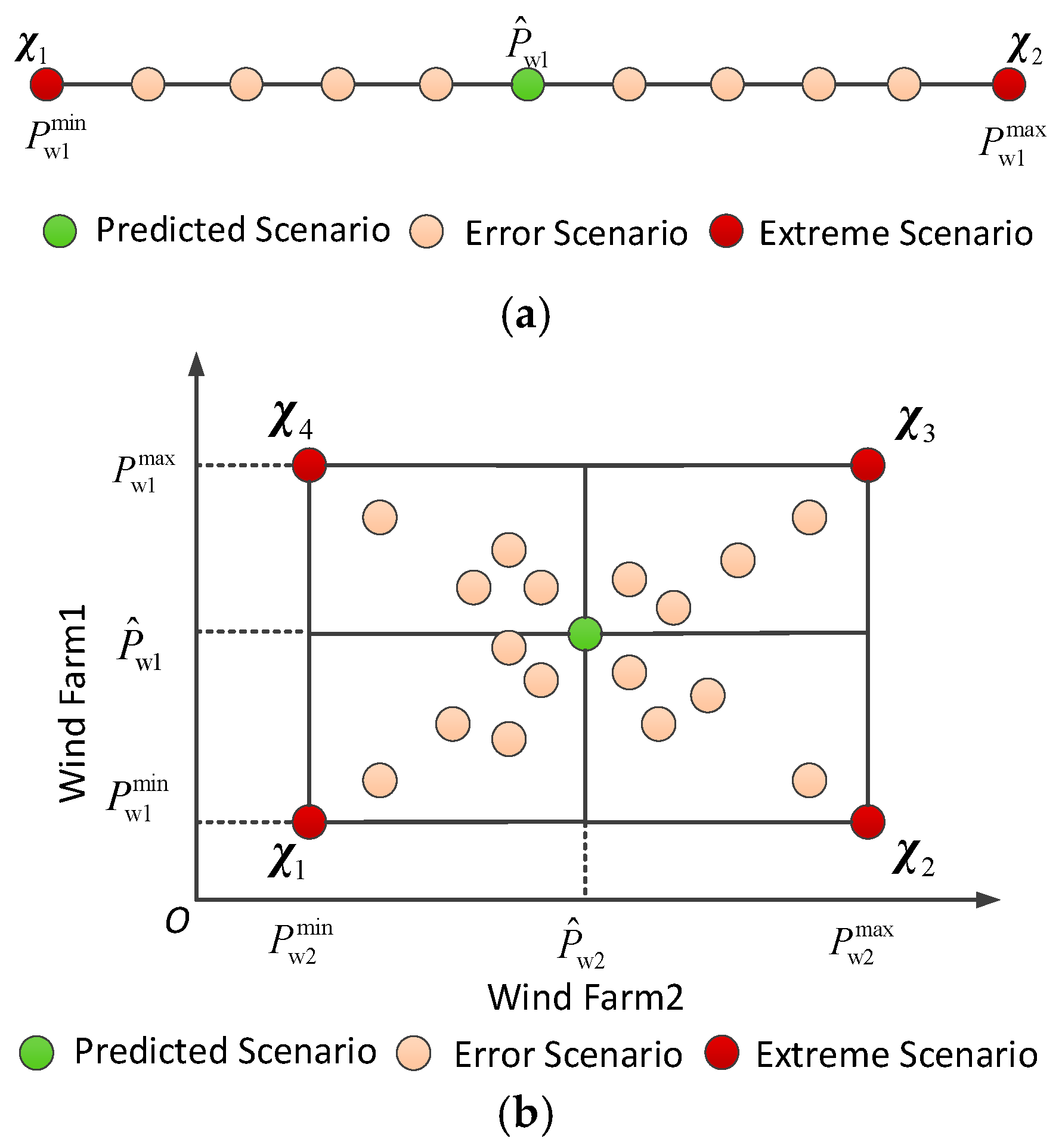
However, it must be noted that, from the perspective of mathematical optimization, an unlimited number of wind power error scenarios will correspond to an unlimited number of operation constraints in the second stage, and problems with unlimited constraints are generally not solvable. Therefore, the present approach attempts to obtain a limited number of discrete scenarios with which to represent the entire wind power output scenario space. To this end, we define extreme scenarios as the boundary condition that constrains possible wind power outputs under all possible fluctuation scenarios. This scenario space is illustrated in Figure 1 for one wind farm and two wind farms.

In Figure 1, $P_w^{\min }$ and $P_w^{\max }$ denotes the lower and upper bounds of confidence interval in a wind farm respectively, and ${\widehat{P}}_w$ is the arithmetic mean of $P_w^{\min }$ and $P_w^{\max }$. It should be noted that, $P_w^{\min }$ and $P_w^{\max }$ can be calculated by the probability density function of wind power under a given confidence level. ${\chi }_s\left(s=1,2,3,4\right)$ denotes the extreme scenario that consists of confidence interval bounds of wind farms. For a single wind farm, there exist two extreme scenarios (${\chi }_1$, ${\chi }_2$) and other possible wind generation outputs lie on the line segment between ${\chi }_1$ and ${\chi }_2$. Similarly, for two wind farms, we can obtain four extreme scenarios (${\chi }_1$, ${\chi }_2$, ${\chi }_3$, ${\chi }_4$), and other possible wind generation outputs lie in the rectangle made of ${\chi }_1$, ${\chi }_2$, ${\chi }_3$ and ${\chi }_4$. Thus, the value space of wind generation output will be an n-dimensional convex polyhedron with $2^n$ vertex when there are n (n ≥ 3) wind farms. In addition, the characteristics of this constraining boundary condition are discussed and formally verified as follows.

Theorem 1.

The extreme scenarios are fully representative of all possible error scenarios in the entire wind power output space. Therefore, provided the operation variables for a given decision-making solution of transmission lines can be adapted to extreme scenarios, they can also be adapted to all possible error scenarios in the wind power output space.

Proof of Theorem 1.

Assuming that ${\chi }_1$, ${\chi }_2$, …, ${\chi }_S$ denote extreme scenarios in the wind power output space and $y_1$, $y_2$, …, $y_S$ respectively denote the solutions corresponding to these extreme scenarios, any scenario in the output space can be expressed as a linear combination of extreme scenarios. Thus, for a group of positive rational numbers ${\alpha }_1$, ${\alpha }_2$, …, ${\alpha }_S$, and each error scenario satisfies the following formulation:

$${\chi }_u={\displaystyle \sum _s\left({\alpha }_s{x}_s\right)}$$

(26)

$${\alpha }_1+{\alpha }_2+\cdots +{\alpha }_S=1$$

(27)

Here, ${\alpha }_s\in \left[0,1\right]$, and $s=1,2,\dots ,S$. Both of $h(·)$ and $q(·)$ in (24) are linear functions of $x$, $y$, and $\chi$. Therefore, without loss of generality, they can be expressed as follows:

$$\begin{array}{l}h(y,\chi )=By-C\chi \le 0\\ q(x,y,\chi )=Mx+Ny-O\chi \le 0\end{array}$$

(28)

Here, A, B, C, M, N, and O denote the coefficient matrix of constraints. This can be extended by including $s=1,2,\dots ,S$, which yields the following:

$${\alpha }_{s}B{y}_s-{\alpha }_{s}C{\chi }_s={\alpha }_{s}h(y_s,{\chi }_s)\le 0$$

(29)

$${\alpha }_{s}Mx+{\alpha }_{s}N{y}_s-{\alpha }_{s}O{\chi }_s={\alpha }_{s}q(x,y_s,{\chi }_s)\le 0$$

(30)

This yields the following constraint expressions:

$${\displaystyle \sum _s\left({\alpha }_{s}h(y_s,{\chi }_s)\right)}\le 0$$

(31)

$${\displaystyle \sum _s\left({\alpha }_{s}q(x,y_s,{\chi }_s)\right)}\le 0$$

(32)

According to linear programming theory [36], any point in the feasible region can be linearly expressed by the boundary point $y_1$, $y_2$, …, $y_S$. Thus, a group of positive rational numbers ${\alpha }_1$, ${\alpha }_2$, …, ${\alpha }_S$ exists for which the following equation holds:

$$y_u={\displaystyle \sum _s\left({\alpha }_s{y}_s\right)}$$

(33)

Substituting $x$ with ${\displaystyle \sum _s{\alpha }_{s}x}$ for any scenario in the wind power output space, and similarly for $y$ and $\chi$ we can obtain the following:

$$\begin{array}{ll}q(x,y_u,{\chi }_u)& =h({\displaystyle \sum _s\left({\alpha }_{s}x\right)},{\displaystyle \sum _s\left({\alpha }_s{y}_s\right)},{\displaystyle \sum _s\left({\alpha }_s{\chi }_s\right)})\\ & =M{\displaystyle \sum _s\left({\alpha }_{s}x\right)}+N{\displaystyle \sum _s\left({\alpha }_s{y}_s\right)}-O{\displaystyle \sum _s\left({\alpha }_s{\chi }_s\right)}\\ & ={\displaystyle \sum _s\left({\alpha }_s\left(Mx+N{y}_s-O{\chi }_s\right)\right)}\\ & ={\displaystyle \sum _s\left({\alpha }_{s}q(x,y_s,{\chi }_s)\right)}\le 0\end{array}.$$

(34)

In the same way, we can also prove:

$$h(y_u,{\chi }_u)={\displaystyle \sum _s\left({\alpha }_{s}h(y_s,{\chi }_s)\right)}\le 0,$$

(35)

which concludes our proof of Theorem 1. □

Accordingly, model (25) can be transformed into the following expression:

$$\{\begin{array}{ll}\min & {\displaystyle \sum _{s}F(x,y_s,{\chi }_s)}\\ s.t.& H(x)\le 0\\ & h(y_1,{\chi }_1)\le 0,q(x,y_1,{\chi }_1)\le 0\\ & \hfill ⋮\hfill \\ & h(y_S,{\chi }_S)\le 0,q(x,y_S,{\chi }_S)\le 0\end{array}.$$

(36)

4. Solution of the Proposed Model

4.1. Two-Stage RTEP Method with Benders Decomposition Algorithm

It should be noted that the RTEP model contains a few binary variables and many continuous variables, thus solving the problems as a whole is computationally exhausting and inefficient. Benders decomposition algorithm [37,38,39] is adopted to transform model (36) into a two-stage RTEP model. Accordingly, we first rewrite (36) as follows.

$$\{\begin{array}{l}\underset{x,y}{\min }{c}^{\mathrm{T}}x+b^{\mathrm{T}}y\\ Ax\le e\\ By\le C\chi \\ Mx+Ny\le O\chi \\ x\in \left[0,1\right],y\in {ℝ}^n\end{array}.$$

(37)

Here, the first stage represents the issue of line construction decision making to determine the network topology under the line investment constraints. The second stage is the operation simulation problem under the constraints of extreme scenarios after the determination of the network topology in the first stage. Thus, problem (37) can be written as follows:

$$\{\begin{array}{ll}\underset{x}{\min }& \left(c^{\mathrm{T}}x+b^{\mathrm{T}}y\right)\\ s.t.& Ax\le e\\ & x\in \left[0,1\right]\\ & \underset{y}{\min }{b}^{\mathrm{T}}y\\ & s.t.By\le C\chi \\ & Mx+Ny\le O\chi \\ & y\in R^n\end{array}.$$

(38)

Letting $\lambda$ and $\mu$ denote the Lagrange multiplier vectors of $By\ge C\chi$ and $Mx+Ny\ge O\chi$, respectively, the second-stage sub-problem in (38) can be given according to duality theory as:

$$Sub\left(\lambda ,\mu \right)=\underset{\lambda ,\mu }{\max }{\lambda }^T\left(-C\chi \right)+{\mu }^T\left(Mx-O\chi \right)$$

(39)

subject to the following conditions:

$$\begin{array}{l}-{\lambda }^{T}B-{\mu }^{T}N=b\\ \lambda \ge 0,\mu \ge 0\end{array}$$

(40)

According to strong duality theory [40], when an optimal solution exists for the original sub-problem in (38), an optimal solution will also exist for the dual problem (39)–(40). Furthermore, the objective function value of the original problem is equal to that of the dual problem at the optimal point. After solving the dual problem, we introduce an auxiliary variable $\eta$ to return the valid Benders cut information in (39) to the first-stage master investment problem of (38), as follows:

$$\begin{array}{ll}Mas(x)=& \underset{x}{\min }{c}^{\mathrm{T}}x+\eta \\ & Ax\le e\\ & \eta \ge {\lambda }^T\left(-C\chi \right)+{\mu }^T\left(Mx-O\chi \right)\\ & x\in \left[0,1\right]\end{array}.$$

(41)

Notice that, the dual sub-problem (39)–(40) is a linear programming problem without binary variables, thus it can be solved by the dual simplex algorithm. Also, the master investment model (41) is a mixed-integer programming problem and can be effectively solved by the branch-and-cut algorithm which solves a series of linear programming problems. In our experiments, we implemented the dual simplex algorithm and the branch-and-cut algorithm using the CPLEX solver [41].

4.2. Summary of the Two-Step RTEP Solution Algorithm

An iterative procedure based on the Benders decomposition algorithm is proposed to solve the two-stage RTEP problem. Master problem (41) is solved at each iteration to update the lower bound of the optimal value with progressively increasing values, and to provide new values for the first stage variables. For given values for the first stage variables, the sub-problem is solved at each iteration to obtain progressively decreasing values of the upper bound of the optimal value. The algorithm terminates after the gap between the lower and upper bounds falls below a preset convergence tolerance $\epsilon$ (here, $\epsilon ={10}^{-6}$ in the present work). A flow chart of the algorithm is summarized in Figure 2, and the proposed iterative steps are described in detail as follows:

(1)

Initialization: Set the value of $\epsilon$. Initialize the upper bound (UB) and lower bound (LB) to $UB=+\infty$ and $LB=-\infty$, and set the iteration counter to l = 1.

(2)

Initial Solution: Prior to conducting iterations, a feasible decision-making solution is first computed. This can be obtained by solving the deterministic TEP without considering wind power uncertainty, where the wind power output is set at the predicted values.

(3)

Sub-problem: Solve the dual problem (39)–(40) by LP for given values of decision-making variables to obtain the optimal dual variables (${\lambda }^{\ast },{\mu }^{*}$). Compute Benders cut information and return it to (41). Update the upper bound as $UB=c^{\mathrm{T}}{x}^{*}+Sub\left({\lambda }^{*},{\mu }^{*}\right)$.

(4)

Master Problem: Add Benders cut information into (41), and then solve (41) by MIP to obtain the optimal master problem variables ($x^{\ast },{\eta }^{*}$). Update the lower bound as $LB=c^{\mathrm{T}}{x}^{*}+{\eta }^{*}$.

(5)

Convergence Checking: If $\left(UB-LB\right)/UB\le \epsilon$, terminate iterations and return the optimal solution. Otherwise, update the iteration counter as $l\to l+1$, and return to Step 3.

5. Numerical Studies

In this section, we analyze the results of numerical studies to determine the effectiveness of the proposed RTEP model in comparison with the results obtained for the conventional TEP (CTEP) method that neglects to account for wind power uncertainty and the costs of pollutant emissions. We first consider Garver’s 6-bus system [42] to illustrate the performance of the proposed extreme-scenario-based method. We then consider the IEEE reliability test system (RTS-79) [43] to investigate the low-emission performance of the proposed model. We employed the Monte Carlo method for both systems to generate 8760 wind power scenarios in the operational simulations of the obtained solutions. In addition, we employed two distinct types of operation simulations, including stochastic operation simulation (SOS) and extreme operation simulation (EOS). In this paper, EOS is defined as the scenarios with the worst operation cost in all possible simulation scenarios, which is contained in the extreme scenario set. For simplicity, the valve-point effects are not considered in numerical studies. The proposed two-stage solution algorithm for the RTEP model is implemented using the commercial General Algebraic Modeling System (GAMS-24.4) mathematical optimization software [41]. The MIP solutions of the master problem and the LP solutions of the sub-problem are obtained using the CPLEX solver. All of the experiments were conducted on a personal computer equipped with an IntelR Dual-coreTM i5 Duo Processor (2.6 GHz) and 8 GB of RAM.

5.1. Garver’s 6-Bus System

5.1.1. Experimental Setting

The topology of Garver’s 6-bus system is depicted in Figure 3, and includes six buses, three generators, and six lines. Two 300 MW wind farms are located at bus # 6. Up to three transmission lines can be installed in each existing corridor or candidate corridor except for corridors 2–6 and 3–5, which can include up to four lines. The construction cost of transmission lines is set to $1.5\times {10}^5$ $/mile, the discount rate is 10%, and the service life of transmission lines is 10 years. We set the cost coefficients of load shedding and wind power curtailment at 1600 $/MWh and 150 $/MWh, respectively. The maximum percentage of wind power curtailment is restricted to not more than 15%. The network parameters is presented in

Table 1. Branch parameters for Garver’s 6-bus system.

From-To	nijmin	nijmax	bij,k (p.u.)	Fijmax (p.u.)	From-To	nijmin	nijmax	bij,k (p.u.)	Fijmax (p.u.)
1–2	1	3	2.5000	1.00	2–6	0	4	3.3333	1.00
1–3	0	3	2.6316	1.00	3–4	0	3	1.6949	0.82
1–4	1	3	1.6667	0.80	3–5	1	4	5.0000	1.00
1–5	1	3	5.0000	1.00	3–6	0	3	2.0833	1.00
1–6	0	3	1.4706	0.70	4–5	0	3	1.5873	0.75
2–3	1	3	5.0000	1.00	4–6	0	3	3.3333	1.00
2–4	1	3	2.5000	1.00	5–6	0	3	1.6393	0.78
2–5	0	3	3.2258	1.00	-	-	-	-	-

. All of the other information regarding the locations of loads and generators can be found elsewhere [42]. The wind power fluctuation was set to 40%, and the output was uniformly distributed in the interval.

5.1.2. Comparison and Analysis of Optimal Results

The results obtained for the two methods under different simulation scenarios are presented as

Table 2. Results of the proposed RTEP method and the conventional TEP (CTEP) method for Garver’s 6-bus system ¹.

OST	TEPM	OPS	NIL	IC ($)	WPC (MWh)	LS (MWh)	OC ($)	CC ($)
SOS	CTEP	2–6(3), 3–5, 4–6(2)	6	6.64 × 106	4.03 × 105	0	5.4345 × 108	5.5009 × 108
	RTEP	2–6(4), 3–5, 4–6(3)	8	8.98 × 106	2.62 × 104	0	4.3427 × 108	4.4326 × 108
EOS	CTEP	2–6(3), 3–5, 4–6(2)	6	6.64 × 106	7.14 × 105	0	6.3629 × 108	6.4293 × 108
	RTEP	2–6(4), 3–5, 4–6(3)	8	8.98 × 106	7.85 × 104	0	4.5201 × 108	4.6099 × 108

¹ OST denotes the operation simulation type, including the stochastic operation simulation (SOS) and the extreme operation simulation (EOS). TEPM denotes the TEP method. OPS denotes the optimal planning solution obtained with the corresponding planning method. NIL denotes the total number of newly installed lines. WPC and LS respectively denote the extent of wind power curtailment and load shedding. IC, OC, and CC denote the investment costs for new lines, the operation costs, and the comprehensive costs, respectively.

. The proposed RTEP method provides an optimal solution that is immune to the realization of all of the possible extreme wind power scenarios. As shown in Figure 3 and Table 2, the proposed RTEP method constructs more transmission lines connected to wind farm node 6 than the CTEP method, and two additional circuit transmission lines 2–6 and 4–6 are accordingly selected. Thus, the investment costs for new lines is increased by 2.34 × 10⁶ $ using the proposed RTEP method. However, while the proposed RTEP method includes higher investment costs, it effectively improves the ability of planning solutions to accommodate wind power output uncertainty. Thus, the proposed RTEP method significantly reduces the quantity of wind power curtailment and the operation costs in the SOS, which therefore reduces the comprehensive costs by 19.42% relative to those of the CTEP method. In contrast to the SOS results, both the CTEP and RTEP methods result in higher wind power curtailment, operation costs, and comprehensive costs under the EOS. However, the RTEP method can take extreme scenarios into account in the optimization process. Therefore, compared with CTEP method, the proposed RTEP method reduces the wind power curtailment and the operation costs by 6.355 × 10⁵ MWh and 1.8428 × 10⁸ $, respectively. Moreover, the proposed RTEP method demonstrates a prominent advantage in terms of the comprehensive costs obtained under extreme operation conditions, where the comprehensive costs are reduced by 28.30% relative to those of the CTEP method.

Both the SOS and EOS results indicate that the RTEP solution includes some degree of wind power curtailment, rather than incorporating all of the possible wind power fluctuations. However, it should be noted that an optimization that simply pursues the goal of incorporating all of the wind power without any curtailment does not always provide an optimal solution in terms of both investment costs for new lines and the capacity for accommodating wind power. In fact, allowing for some degree of wind power curtailment may be more conducive toward obtaining an optimal decision-making solution. Actually, the RTEP method can be regarded as a competitive process between concerns related to investment costs and the capacity for accommodating wind power. Here, although a solution suggesting the construction of fewer new lines can reduce investment costs, the correspondingly decreased capacity for accommodating wind power may lead to greater wind power curtailment. Conversely, a solution suggesting the construction of additional new lines increases the capacity for accommodating wind power, resulting in reduced wind power curtailment. However, the installation of additional new lines increases the investment costs. To some extent, the RTEP method searches for a solution that represents a reasonable trade-off between line investment and wind power capacity.

5.1.3. Analysis of Wind Farm Location

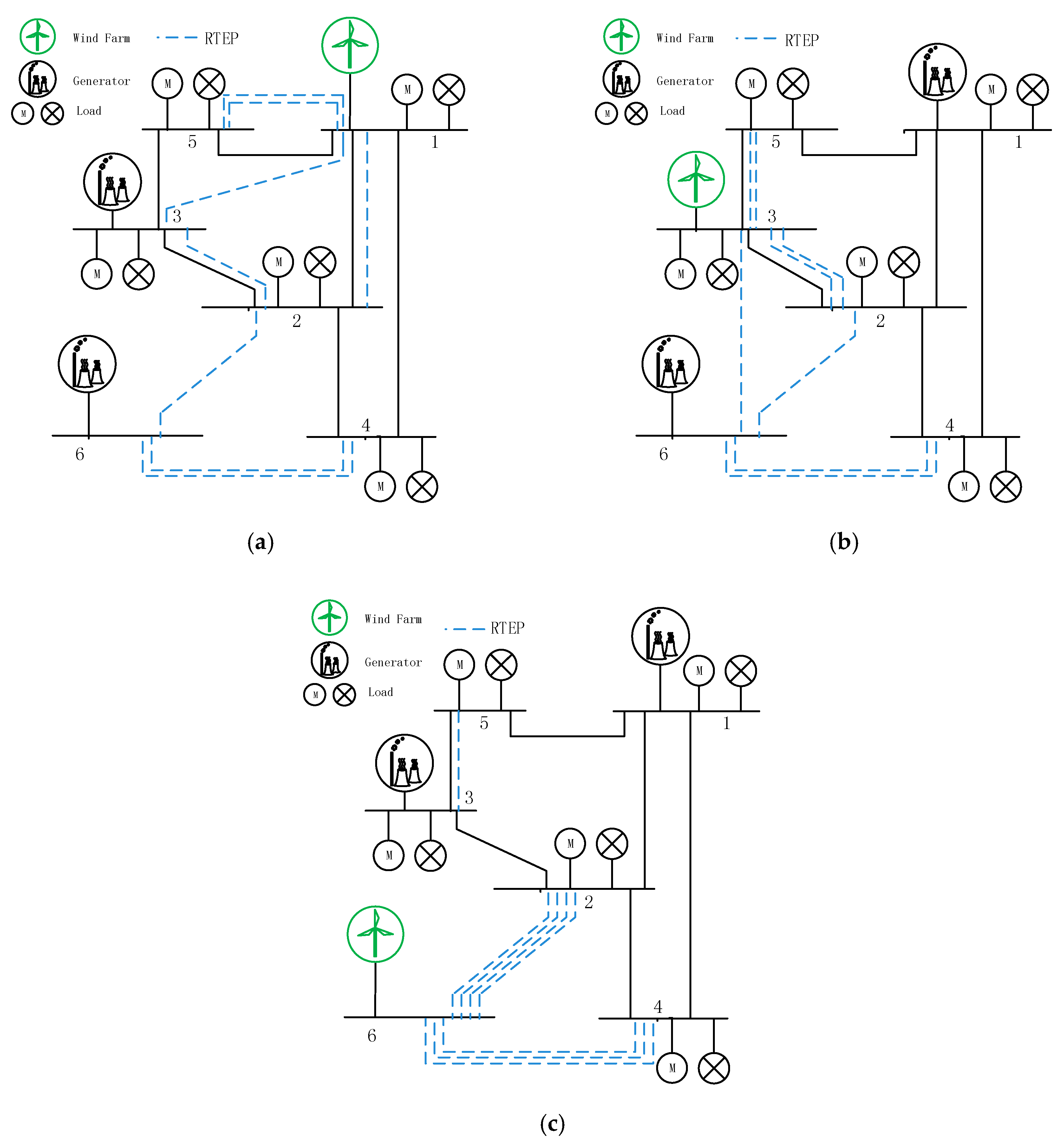
To illustrate the impact of different wind farm locations on the RTEP solution, we test the RTEP model under three location scenarios of wind farms and conventional generators: (1) scenario # 1: wind farms are located at bus # 1, and conventional generators are located at buses # 3 and # 6; (2) scenario # 2: wind farms are located at bus # 3, and conventional generators are located at buses # 1 and # 6; (3) scenario # 3: wind farms are located at bus # 6, and conventional generators are located at buses # 1 and # 3. The SOS results of RTEP obtained under different wind farm location scenarios are listed in

Table 3. RTEP results obtained under different wind farm locations.

Scenarios	NIL	IC ($)	WPC (MWh)	LS (MWh)	OC ($)	CC ($)
Scenario # 1	8	8.91 × 106	0	0	4.2668 × 108	4.3559 × 108
Scenario # 2	8	8.51 × 106	0	5.36 × 103	4.3452 × 108	4.4303 × 108
Scenario # 3	8	8.98 × 106	2.62 × 104	0	4.3427 × 108	4.4326 × 108

, and the detailed selected transmission line solutions are presented in Figure 4.

It can be seen in Table 3 and Figure 4 that although the obtained solutions under different location scenarios have the same number of newly installed lines, the specific locations of the proposed transmission lines and the total investment costs for newly installed lines are quite different. The highest investment costs are found in scenario # 3 where wind farms are located at bus # 6, because bus # 6 is isolated and far away from the controllable generators and loads, compared with the other two scenarios. Note that, more than half selected transmission lines have relation with the bus with wind power integration in all obtained solutions. The transmission lines connected to wind farm bus are more inclined to be selected for construction, for the purpose of promoting wind power consumption and reducing wind power curtailment. Thus, in practice, to improve the capacity of wind power consumption, an appropriate location should be considered when we carry out wind farm planning.

5.1.4. Analysis of Wind Power Fluctuations

To illustrate the impact of different levels of wind power fluctuation on the RTEP solution, we employed the wind power deviation intensity $\beta$ to characterize the maximum degree of wind power fluctuation. Here, $\beta$ is defined as the maximum percentage that the actual output of wind power $P_{i,w}^{\mathrm{W}}$ deviates from its predicted output ${\widehat{P}}_{i,w}^{}$, which can be expressed as follows:

$$\beta =\max \left(\frac{\left|P_{i,w}^{\mathrm{W}}-{\widehat{P}}_{i,w}\right|}{{\widehat{P}}_{i,w}}\right)$$

(42)

For the sake of simplicity, it is assumed that a single value of $\beta$ applies to all wind farms. Note that, the predicted output ${\widehat{P}}_{i,w}$ is a fixed value, which can be obtained by multiple wind power forecasting technologies [44], i.e., artificial neural network method, support vector machine regression method, neuro-fuzzy network method, etc. Thus, the value of $\beta$ is determined by $P_{i,w}^{\mathrm{W}}$, and $\beta$ obtains its maximum value when wind power $P_{i,w}^{\mathrm{W}}$ reaches the lower or upper bounds of confidence interval. That is, $\beta =\left(P_{i,w}^{\max }-{\widehat{P}}_{i,w}\right)/{\widehat{P}}_{i,w}=\left({\widehat{P}}_{i,w}-P_{i,w}^{\min }\right)/{\widehat{P}}_{i,w}$. It should be noted that, $\beta$ can greatly influence the obtained solutions via the values of $P_{i,w}^{\max }$ and $P_{i,w}^{\min }$. For a given confidence level, the value of $\beta$ reflects accurate wind power forecasting technology to a certain extent. The results of RTEP obtained under different values of $\beta$ are listed in

Table 4. RTEP results obtained under different levels of wind power deviation intensity $\beta$.

$\mathit{\beta }$	IC ($)	WPC (MWh)	LS (MWh)	OC ($)	CC ($)
0%	6.64 × 106	0	0	4.2924 × 108	4.3588 × 108
20%	7.81 × 106	0	0	4.2924 × 108	4.3705 × 108
40%	8.98 × 106	7.85 × 104	0	4.5201 × 108	4.6099 × 108
60%	1.0858 × 107	8.58 × 104	2.30 × 105	7.9049 × 108	8.0135 × 108
74%	NA 2	NA	NA	NA	NA

² This indicates that an RTEP solution was not available (NA).

.

It can be seen from Table 4 that the investment costs for new lines increases with increasing $\beta$, and the optimal solution becomes increasingly conservative for the sake of accommodating stochastic fluctuations in wind power, and for promoting the effective integration of wind power. For $\beta$ ≤ 20%, the solutions can fully accommodate the stochastic fluctuations in the wind power, and no wind power curtailment or load shedding is required during operation. In contrast, we note that an increasing degree of wind power curtailment and/or load shedding is required for $\beta$ > 20%, which indicates that the additional investment costs that would be required for incorporating all wind power without any curtailment are greater than the costs associated with the adopted degree of wind power curtailment and load shedding. Thus, it is preferable to adopt a partial abandonment of wind power, rather than continuing to increase the investment costs for new lines. In addition, the absence of a feasible solution for $\beta$ = 74% indicates that the range of wind power fluctuation that can be accommodated by the planning model has limits due to the limited number of candidate corridors and transmission lines. Thus, in practice, an appropriate value of $\beta$ should be secured via accurate wind power forecasting technology and the experience of TSOs.

In this paper, we define the extreme wind power deviation intensity as the maximum value of $\beta$ that the planning model can accommodate. Then, we investigated the effect of the degree of wind power penetration on the extreme wind power deviation intensity. This effect was investigated for five levels of wind power penetration, and the results are presented in Figure 5.

It can be observed from Figure 5 that the maximum value of $\beta$ that the planning model can accommodate decreases significantly with increasing wind power penetration. The reasons for this are expected to be twofold: (i) the upper limit on the number of candidate corridors and transmission lines that the system can include limits the total possible quantity of wind power that the system can accommodate. Thus, wind power fluctuations are increasingly restricted with increasing wind power penetration; (ii) the relative proportion of flexible resources (i.e., coal-fired generators and gas-fired generators) decreases with increasing wind power penetration, and a lower proportion of flexible resources limits the ability of the system to accommodate extreme wind power fluctuations. These results suggest that increasing the number of candidate transmission lines or increasing the penetration of flexible resources can increase the maximum value of $\beta$ that the planning model can accommodate to some extent.

5.2. IEEE RTS-79 System

The modified IEEE RTS-79 system includes 38 existing lines, 85 candidate lines, and 25 generators. Buses # 2, # 7, and # 22 are respectively connected with six, four, and six wind turbines, each with a rated capacity of 350 MW, and the wind power penetration was 52.1%, which represents a typical high-penetration wind power system. The other buses are connected with conventional coal-fired generators, except for bus # 23, to which three 500 MW gas-fired generators are connected. All of the other information regarding network parameters and the locations of loads and generators can be found elsewhere [43]. The pollutant emission coefficients of the individual generator types are listed in

Table 5. Pollutant emission coefficients for individual generator types.

Pollutant Emissions		CO	CO2	SO2	NOx
Treatment Costs ($·kg−1)		1.160	0.033	7.283	9.687
Pollutant Emission Coefficient (kg·(MWh)−1)	Wind Turbine	0.000	0.000	0.000	0.000
	Coal-fired Generator	0.140	834.746	0.514	4.007
	Gas-fired Generator	0.000	402.000	0.003	0.010

[45,46].

Here, it should be noted that the generation costs and emission characteristics of gas-fired and coal-fired generators are quite different. Gas-fired generators have a greater generation cost, but environmental pollution costs are reduced due to their low-emissions characteristics (i.e., CO, CO₂, SO₂ and NO_x). In contrast, although coal-fired generators have a relatively low generation cost, greater environmental pollution costs are incurred per equivalent power generation because they generate more emissions during the power generation process.

5.2.1. Comparison and Analysis of Optimal Results

A comparison of the results obtained for the two methods under different simulation scenarios are listed in

Table 6. Results of the proposed RTEM method and the CTEP method for the IEEE RTS-79 system.

OST	TEPM	IC ($)	WPC (MWh)	LS (MWh)	OC ($)	CC ($)
SOS	CTEP	8.4840 × 107	6.1977 × 106	8.9919 × 105	1.4260 × 1010	1.4340 × 1010
	RTEP	1.7107 × 108	1.0888 × 106	0	5.0387 × 109	5.2098 × 109
EOS	CTEP	8.4840 × 107	1.3224 × 107	9.1702 × 105	2.3532 × 1010	2.3617 × 1010
	RTEP	1.7107 × 108	2.9958 × 106	0	9.1450 × 109	9.3161 × 109

. In terms of the investment costs for transmission lines, the proposed RTEP method constructed 15 more transmission lines to accommodate the uncertainty associated with a high penetration of wind power than the CTEP method, which accordingly increased the investment costs for new lines by 8.623 × 10⁷ $. As for operation costs, the RTEP solutions significantly reduced the extent of wind power curtailment and load shedding under both SOS or EOS conditions. Thus, the proposed RTEP method effectively improved the robustness of the solution for accommodating wind power fluctuations, and the operation costs were reduced significantly. Specifically, the operation costs of the proposed RTEP method under SOS and EOS conditions were respectively reduced by 9.2213 × 10⁹ $ and 1.4387 × 10⁹ $ relative to the corresponding operation costs of the CTEP method. Overall, the decrease in operation costs was much greater than the increase in investment costs, such that the proposed RTEP method demonstrated a prominent advantage with respect to comprehensive costs.

5.2.2. Analysis of Environmental Pollution

As discussed, the environmental pollution costs associated with power generation is embedded in the objective function of the proposed RTEP model, and the impact of environmental pollution on RTEP solutions is illustrated by comparing the planning results and pollutant emissions obtained with the RTEP model with those obtained with the CTEP method that neglects environmental pollution costs. The results are listed in

Table 7. Results of the proposed low-emission RTEP method and the CTEP method for the IEEE RTS-79 system.

TEPM	LA 3	NIL	Pollutant Emissions (kg)				OC ($)	CC ($)
			CO	CO2	SO2	NOx
RTEP	9–11, 10–11, 19–23	36	1.6254 × 104	1.4019 × 108	5.9997 × 104	4.6628 × 105	5.0387 × 109	5.2098 × 109
CTEP	13–14, 15–24, 16–19	36	3.0605 × 104	1.8433 × 108	1.1238 × 105	8.7600 × 105	5.3300 × 109	5.4905 × 109

³ LA denotes the different transmission lines added by the two decision-making solutions.

.

It should be noted from Table 7 that, although the RTEP and CTEP solutions construct the same number of transmission lines, the specific locations of the proposed transmission lines differ, and the investment costs for new lines are slightly higher for RTEP than for CTEP. This is because the CTEP solution is obtained without considering the environmental pollution costs associated with generator infrastructure. Thus, the optimal solution is more inclined to construct transmission lines 13–14, 15–24, and 16–19 connected to the coal-fired generator buses at buses # 13, # 15, and # 16 because of the lower generation cost of coal-fired generators compared with that of gas-fired generators. In contrast, the low-emission characteristics of gas-fired generators are taken into account in the RTEP solution, such that the obtained optimal solution is more likely to invest in transmission lines connected with gas-fired generators to reduce emissions. Furthermore, we note from Table 5 that the CO, CO₂, SO₂, and NO_x emissions obtained by the proposed RTEP method are significantly reduced by 46.89%, 23.95%, 46.61%, and 46.77%, respectively, relative to those obtained by the CTEP method. In addition, we note that the operation costs and comprehensive costs obtained by the proposed RTEP approach are respectively 5.47% and 5.11% less than those obtained by the CTEP model. Therefore, the RTEP approach can yield economic benefits for TEP solutions, and demonstrates good engineering application value.

5.3. IEEE 118-Bus System

To show the applicability of proposed RETP method, we test the large-scale case based on the modified IEEE 118-bus system in this part. The system comprises 118 buses, 186 existing lines, 61 candidate lines, 54 generators, and 94 loads. Buses # 49, # 77, and # 100 are respectively connected with seven, four, and five wind turbines, each with a rated capacity of 350 MW. All of the other information regarding the network parameters and the locations of loads and generators can be found elsewhere [47]. The results obtained for the two methods under different simulation scenarios are presented as

Table 8. Results of the proposed RTEM method and the CTEP method for the IEEE 118-bus system.

OST	TEPM	IC ($)	OC ($)	CC ($)
SOS	CTEP	8.8575 × 107	9.295 × 1010	9.3036 × 1010
	RTEP	1.4177 × 108	9.282 × 1010	9.2958 × 1010
EOS	CTEP	8.8575 × 107	9.623 × 1010	9.6322 × 1010
	RTEP	1.4177 × 108	9.401 × 1010	9.4147 × 1010

.

In terms of the investment costs for transmission lines, the proposed RTEM method increased the investment costs for new lines by 5.3195 × 10⁷ $ compared with CTEP method, since more transmission lines are selected for construction to accommodate wind power uncertainty. However, the proposed RTEP solutions could effectively improve the robustness of the solution for accommodating wind power fluctuations, and significantly reduce the operation costs. As a whole, the decrease in operation costs was much greater than the increase in investment costs, such that the proposed RTEP method demonstrated a prominent advantage with respect to comprehensive costs. Specifically, the comprehensive costs of proposed RTEP method under SOS and EOS conditions were respectively reduced by 7.8 × 10⁷ $ and 2.2 × 10⁹ $ relative to the corresponding operation costs of the CTEP method.

6. Conclusions

This paper proposed a novel definition of extreme scenarios for conducting TEP with high wind power penetration and wind power output uncertainty. It was theoretically proven that decision-making solutions adaptable to extreme scenarios in the wind power output space can be adapted to all possible error scenarios therein. Extreme scenarios were then adopted to establish a two-stage robust TEP model that considers the pollution emissions of the generation infrastructure. Here, the first-stage optimization pertains to the issue of line construction decision making, and the second-stage optimization represents the operation simulation problem under the constraints of extreme scenarios. The proposed model avoids the emergence of non-convex bilinear terms that can arise in conventional robust TEP methods, while ensuring that the obtained solutions can accommodate any degree of wind power fluctuation. Numerical studies conducted with Garver’s 6-bus system, a modified IEEE RTS-79 system and IEEE 118-bus system demonstrated the good applicability and robustness of the proposed model. The detailed conclusions of the study are given below:

(1)

Compared with the CTEP model, the proposed RTEP model can effectively reduce operation costs and the extent of wind power curtailment, and therefore yields lower comprehensive costs. Moreover, the proposed RTEP method demonstrates a prominent advantage in terms of comprehensive costs under both the SOS and EOS.

(2)

The decision-making solutions obtained by RTEP exhibit increasing costs associated with line investment, wind power curtailment, and load shedding with the increasing extent to which the actual wind power output deviates from its predicted output. This limits the maximum extent of this deviation that can be accommodated by the planning solutions obtained by RTEP to a value that decreases with increasing wind power penetration.

(3)

Compared with the CTEP model, the proposed RTEP model can significantly reduce the pollution emissions of power generation.

This study is a first attempt to build the extreme scenario based TEP model incorporating the uncertainty of wind power. Apart from its advantages, it inevitably has certain drawback. The computational cost will largely increase when the model is employed to the large-scale power system with wind power uncertainty. In addition, the proposed model mainly focuses on the uncertainty of wind power. Further research can extend the model to accommodate more complex uncertain factors.

References

- Zhou, S.; Wang, Y.; Zhou, Y.; Clarke, L.E.; Edmonds, J.A. Roles of wind and solar energy in China’s power sector: Implications of intermittency constraints. Appl. Energy 2018, 213, 22–30. [Google Scholar] [CrossRef]
- Sun, X.; Zhang, B.; Tang, X.; McLellan, B.; Höök, M. Sustainable energy transitions in china: Renewable options and impacts on the electricity system. Energies 2016, 9, 980. [Google Scholar] [CrossRef]
- Chen, X.; Mcelroy, M.; Kang, C. Integrated energy systems for higher wind penetration in china: Formulation, implementation and impacts. IEEE Trans. Power Syst. 2017, 33, 1309–1319. [Google Scholar] [CrossRef]
- Mutale, J.; Strbac, G. Transmission network reinforcement versus FACTS: An economic assessment. IEEE Trans. Power Syst. 2000, 15, 961–967. [Google Scholar] [CrossRef]
- Dusonchet, Y.P.; Elabiad, A. Transmission planning using discrete dynamic optimizing. IEEE Trans. Power Appar. Syst. 1973, 92, 1358–1371. [Google Scholar] [CrossRef]
- Li, X.; Li, Y.; Zhu, X. Generation and transmission expansion planning based on game theory in power engineering. Syst. Eng. Procedia 2012, 4, 79–86. [Google Scholar]
- Bahiense, L.; Oliveira, G.C.; Pereira, M.; Granville, S. A mixed integer disjunctive model for transmission network expansion. IEEE Trans. Power Syst. 2001, 16, 50–60. [Google Scholar] [CrossRef]
- Haffner, S.; Monticelli, A.; Garcia, A.; Mantovani, J.; Romero, R. Branch and bound algorithm for transmission system expansion planning using a transportation model. IEE Gener. Transm. Distrib. 2000, 147, 149–156. [Google Scholar] [CrossRef]
- Silva, A.M.L.D.; Rezende, L.S.; Manso, L.A.D.F. Reliability worth applied to transmission expansion planning based on ant colony system. Int. J. Electr. Power Energy Syst. 2010, 32, 1077–1084. [Google Scholar] [CrossRef]
- Kuo, T.; Ming, Z.; Fan, Y. Chance constrained transmission system expansion planning method based on chaos quantum honey bee algorithm. In Proceedings of the IEEE Asia-Pacific Power and Energy Engineering Conference (APPEEC), Chengdu, China, 28–31 March 2010; Available online: https://www.infona.pl/resource/bwmeta1.element.ieee-art-000005448170 (accessed on 9 August 2018).
- Zhao, J.; Dong, Z.; Lindsay, P. Flexible transmission expansion planning with uncertainties in an electricity market. IEEE Trans. Power Syst. 2009, 24, 479–488. [Google Scholar] [CrossRef]
- Rezende, L.; da Silva, A.; de Mello Honório, L. Artificial immune system applied to the multi-stage transmission expansion planning. Artif. Immune Syst. 2009, 5666, 178–191. [Google Scholar]
- Eghbal, M.; Saha, T.K.; Hasan, K.N. Transmission expansion planning by meta-heuristic techniques: A comparison of Shuffled Frog Leaping Algorithm, PSO and GA. In Proceedings of the IEEE Power and Energy Society General Meeting, Detroit, MI, USA, 24–29 July 2011. [Google Scholar]
- Park, H.; Baldick, R. Transmission planning under uncertainties of wind and load: Sequential approximation approach. IEEE Trans. Power Syst. 2013, 28, 2395–2402. [Google Scholar] [CrossRef]
- Sun, C.; Bie, Z.; Xie, M.; Ning, G. Effects of wind speed probabilistic and possibilistic uncertainties on generation system adequacy. IET Gener. Trans. Distrib. 2014, 9, 339–347. [Google Scholar] [CrossRef]
- Hemmati, R.; Hooshmand, R.A.; Khodabakhshian, A. Coordinated generation and transmission expansion planning in deregulated electricity market considering wind farms. Renew. Energy 2016, 85, 620–630. [Google Scholar] [CrossRef]
- Saboya, G.L.; Quelhas, O.L.G.; Caiado, R.G.G.; Franca, S.L.B. Monte Carlo simulation for planning and decisions making in transmission project of electricity. IEEE Latin Am. Trans. 2017, 15, 31–438. [Google Scholar]
- Qiu, J.; Zhao, J.; Wang, D. Flexible multi-objective transmission expansion planning with adjustable risk aversion. Energies 2017, 10, 1036–1053. [Google Scholar] [CrossRef]
- Zheng, Q.P.; Wang, J.; Liu, A.L. Stochastic optimization for unit commitment—A review. IEEE Trans. Power Syst. 2015, 30, 1913–1924. [Google Scholar] [CrossRef]
- Yu, H.; Chung, C.Y.; Wong, K.P.; Zhang, J.H. A chance constrained transmission network expansion planning method with consideration of load and wind farm uncertainties. IEEE Trans. Power Syst. 2009, 24, 1568–1576. [Google Scholar] [CrossRef]
- Qiu, J.; Dong, Z.Y.; Zhao, J.; Xu, Y.; Luo, F. A risk-based approach to multi-stage probabilistic transmission network planning. IEEE Trans. Power Syst. 2016, 31, 4867–4876. [Google Scholar] [CrossRef]
- Hong, S.; Cheng, H.; Zeng, P. An N-k analytic method of composite generation and transmission with interval load. Energies 2017, 10, 168. [Google Scholar] [CrossRef]
- Li, C.X.; Dong, Z.Y.; Chen, G.; Luo, F.J.; Liu, J. Flexible transmission expansion planning associated with large-scale wind farms integration considering demand response. IET Gener. Trans. Distrib. 2015, 9, 2276–2283. [Google Scholar] [CrossRef]
- Li, Y.; Wang, J.; Ding, T. Clustering-based chance-constrained transmission expansion planning using an improved benders decomposition algorithm. IET Gener. Trans. Distrib. 2018, 12, 935–946. [Google Scholar] [CrossRef]
- Jabr, R.A. Robust transmission network expansion planning with uncertain renewable generation and loads. IEEE Trans. Power Syst. 2013, 28, 4558–4567. [Google Scholar] [CrossRef]
- Chen, B.; Wang, J.; Wang, L.; He, Y.; Wang, Z. Robust optimization for transmission expansion planning: minimax cost vs. minimax regret. IEEE Trans. Power Syst. 2014, 29, 3069–3077. [Google Scholar] [CrossRef]
- Zhang, X.; Conejo, A.J. Robust transmission expansion planning representing long-and short-term uncertainty. IEEE Trans. Power Syst. 2018, 33, 1329–1338. [Google Scholar] [CrossRef]
- Mínguez, R.; García-Bertrand, R. Robust transmission network expansion planning in energy systems: Improving computational performance. J. Oper. Res. 2015, 126, 21–32. [Google Scholar] [CrossRef]
- Dehghan, S.; Amjady, N.; Conejo, A.J. Adaptive robust transmission expansion planning using linear decision rules. IEEE Trans. Power Syst. 2017, 32, 4024–4034. [Google Scholar] [CrossRef]
- Konno, H. A cutting plane algorithm for solving bilinear programs. Math. Program. 1976, 11, 14–27. [Google Scholar] [CrossRef] [Green Version]
- Naderi, E.; Azizivahed, A.; Narimani, H.; Fathi, M.; Narimani, M.R. A comprehensive study of practical economic dispatch problems by a new hybrid evolutionary algorithm. Appl. Soft Comput. 2017, 61, 1186–1206. [Google Scholar] [CrossRef]
- Rathore, C.; Roy, R. Impact of wind uncertainty, plug-in-electric vehicles and demand response program on transmission network expansion planning. Int. J. Electr. Power Energy Syst. 2016, 75, 59–73. [Google Scholar] [CrossRef]
- Carrion, M.; Arroyo, J.M. A computationally efficient mixed-integer linear formulation for the thermal unit commitment problem. IEEE Trans. Power Syst. 2006, 21, 1371–1378. [Google Scholar] [CrossRef]
- Ding, H.; Zhang, Y.; Gole, A.M.; Woodford, D.A.; Han, M.X. Analysis of coupling effects on overhead VSC-HVDC transmission lines from AC lines with shared right of way. IEEE Trans. Power Deliv. 2011, 25, 2976–2986. [Google Scholar] [CrossRef]
- Glover, J.D.; Sarma, M.S.; Overbye, T. Power System Analysis & Design, SI Version; Cengage Learning: Boston, MA, USA, 2012; ISBN 9781111425791. [Google Scholar]
- Boyd, S.; Vandenberghe, L. Convex Optimization; Cambridge University Press: Cambridge, UK, 2004; ISBN 9780521833783. [Google Scholar]
- Benders, J. Partitioning procedures for solving mixed variables programming problems. Numerische Math. 1962, 4, 238–252. [Google Scholar] [CrossRef]
- Wydra, F.M. Performance and accuracy investigation of the two-step algorithm for power system state and line temperature estimation. Energies 2018, 11, 1005. [Google Scholar] [CrossRef]
- Rahmaniani, R.; Crainic, T.G.; Gendreau, M.; Rei, W. The Benders decomposition algorithm: A literature review. J. Oper. Res. 2016, 259, 801–817. [Google Scholar] [CrossRef]
- Rockafellar, R.T. Lagrange multipliers and optimality. Siam Rev. 1993, 35, 183–238. [Google Scholar] [CrossRef]
- Rosenthal, R.E. GAMS, A User’s Guide; GAMS Development Corp: Washington, DC, USA, 2014. [Google Scholar]
- Garver, L.L. Transmission network estimation using linear programming. IEEE Trans. Power Appar. Syst. 1970, 89, 1688–1697. [Google Scholar] [CrossRef]
- Grigg, C.; Wong, P.; Albrecht, P. The IEEE reliability test system-1996, a report prepared by the reliability test system task force of the application of probability methods subcommittee. IEEE Trans. Power Syst. 2002, 14, 1010–1020. [Google Scholar] [CrossRef]
- Colak, I.; Sagiroglu, S.; Yesilbudak, M. Data mining and wind power prediction: A literature review. Renew. Energy 2012, 46, 241–247. [Google Scholar] [CrossRef]
- Zhang, N.; Cai, R. The proper order of magnitude of penalty for pollutant emission. Proc. Chin. Soc. Electr. Eng. 1997, 17, 286–288. [Google Scholar]
- Wan, Y.; Adelman, S. Distributed Utility Technology Cost, Performance, and Environmental Characteristics; Office of Scientific & Technical Information Technical Reports: Washington, DC, USA, 1995.
- IEEE 118-Bus System. 2011. Available online: http://motor.ece.iit.edu/ data/data 118 bus.pdf (accessed on 7 August 2018).
Figure 1.
Schematic of the wind power output scenario space. (a) One wind farm; (b) Two wind farms.
Figure 2.
Flow chart of the two-stage robust TEP (RTEP) solution algorithm.
Figure 3.
Connection diagram of Garver’s 6-bus system.
Figure 4.
RTEP solutions obtained under different wind farm locations. (a) Wind farms located at bus # 1; (b) Wind farms located at bus # 3; (c) Wind farms located at bus # 6.
Figure 5.
Extreme wind power deviation intensity under different degrees of wind power penetration.