Analysis of Propagation Delay for Multi-Terminal High Voltage Direct Current Networks Interconnecting the Large-Scale Off-Shore Renewable Energy

Abstract

Voltage-source-converter-based multi-terminal high voltage direct current (MTDC) networks are extensively recognized as a viable solution for meeting the increasing demand of electrical energy and escalating penetration of renewable energy sources. DC faults are major limitations to the development of MTDC networks. The analysis of variable constraints has become mandatory in order to develop a reliable protection scheme. This paper contributes in assessing the propagation delay with the analytical approximation in MTDC networks. The propagation delay is analyzed in the time domain by taking only the forward traveling wave into account and considering the initial voltage step of magnitude at the fault position. Numerous simulations were carried out for different parameters and arrangements in Power System Computer Aided Design (PSCAD) to explore the proposed expressions. The results accurately depicted the time development of fault current. The results obtained from the real-time digital simulator (RTDS) confirmed that the proposed approach is capable of evaluating propagation delay in MTDC networks. Moreover, the influence of fault resistance is also taken into account for investigating its effect on the system parameters.

1. Introduction

In recent years, the consumption of electrical energy has escalated dramatically. To cope with this increasing demand, the power scales and distances from load centers to power production units have also grown significantly. As per the prediction of the European Energy Association (EEA), by the year 2030, the installed capacity will be inclined up to 150 GW, vide offshore wind projects [1,2]. Moreover, there exists an increasing desire to interconnect various regions of the world, in particular the proposal for a North Sea offshore grid concept [3,4].

Most of the recommended future projects based on offshore wind farms will be located significantly far away from the load centers. Different studies have investigated that the use of traditional high voltage alternating current (HVAC) transmission to interconnect wind farms to the load center becomes progressively expensive as the distance increases and would ultimately become infeasible beyond a particular distance [5,6]. High voltage direct current (HVDC) is expected to be recognized in the development of future offshore projects. Voltage-source converter (VSC) technology offers a wide range of flexibility and power control for the development of HVDC. VSCs are also chosen for employment in a meshed offshore grid or multi-terminal scenarios as compared to the conventional current source converter (CSC) technology that has been extensively used for point-to-point HVDC interconnection projects [7,8].

DC faults are considered as the major limitations in the development of multi-terminal high voltage DC (MTDC) networks. With the occurrence of fault, a voltage surge propagates to the terminating points of the system and the propagation speed of the signal is taken as the speed of light for communications among the relays. Numerous researchers have considered the random propagation speed of 200 km/ms as the speed of light in the optical cable [9,10,11,12,13,14,15,16]. Besides this, if we assume that a line breakage fault occurs, the direct communication delay between converter stations will be affected. In this situation, the communication signal has to travel via other converter stations. Fault detection and selective isolation in the MTDC network is considered through fault wave propagation in Reference [9]. A dedicated communication channel is used for each DC cable to provide support to the communication path between both ends of the cable. A communication delay is taken as a transport delay of the wave propagation and presumed as a light speed of 200 km/ms through the fiber optic transmission line for 600 km. Fault detection for MTDC networks joining large-scale offshore wind farms based on differential current approaches with less fault clearing time is described in Reference [10]. In this study, the communication delay between the over-current relays is considered as 1.5 ms for a 300 km DC cable. Single-ended differential protection scheme for MTDC networks has been presented in Reference [11]. The current is obtained by utilizing the optical measuring sensors distributed along the transmission lines. The sensors are installed every 30 km along the transmission line. In case of a fault adjacent to a sensor, the propagation delay is assumed to be 0.3 ms over a distance of 60 km, which is cogitated for forward and backward traveling waves. Analysis, identification and isolation of faults in MTDC networks have been proposed in References [12,13,14,15]. The propagation delay is considered to be 200 km/ms. A non-communication based protection algorithm for MTDC has been depicted in Reference [16]; however, in this study, the propagation speed is selected as 299.2 km/ms, whereas the delay is considered as 1 ms for a 300 km long DC cable. Due to these considerations, the propagation delay needs meticulously investigation with analytical approximation and validation through real-time hardware tests for standardized calculations.

The basic aim of the paper is to investigate the propagation delay in the MTDC network for connecting the large offshore energy production units. In order to solve the aforementioned problem of assuming the propagation delay, standardized calculations have been done for evaluating the propagation delay among the relaying points in the MTDC network based on the individual surges. Numerous simulations are performed for different arrangements in Power System Computer Aided Design (PSCAD) to investigate the proposed expressions. The results exhibit a precise depiction of the time development of the fault current and propagation of signal. Moreover, results are also validated in real-time digital simulator (RTDS) and the proposed approach be standardized for the evaluation of propagation delay in large MTDC networks.

The remaining paper is structured as follows: Section 2 illuminates the reflection coefficient of cable. Section 3 presents the simulation modeling. Methodology and proposed model for the analysis of propagation delay are discussed in Section 4 and Section 5 respectively. Results and evaluations are expressed in Section 6. Finally, the conclusion is drawn in Section 7.

2. Reflection Coefficient

Pole to ground (P–G) faults are the major frailty in MTDC networks. At the time of ground fault, the current ascends rapidly, meanwhile the voltage of the fault location descends quickly. Moreover, the voltage of the different terminals of MTDC drops within a few milliseconds in accordance with the distance from fault locations. The decrement in voltage at the fault point is rapid, not immediate and is in reverence to distributed capacitance of the cable, and the fault path resistance. The voltage drop depends on the attributes of the soil and its resistivity [17]. In general, the greater the resistance of the fault, the lesser the voltage drop of the cable. If a P–G fault occurs at the center of cable, right after the fault, a negative voltage surge travels in both directions through the cable in the direction of terminating points as depicted in Figure 1a. At the same time, the distributed capacitance of the cable is discharged gradually through the ground fault. Due to capacitive termination of the voltage-source converter (VSC) system, the negative voltage surge reflects back as a positive after arriving at the terminating points. The positive voltage surge is named as the reflected voltage [18], and mathematically described as:

$$v_{ref}(t)=v_{incident}(t)\times \left[-\Delta \partial (t)+\frac{2}{R_{c}C}{e}^{-\frac{t}{R_{c}C}}u(t)\right],$$

(1)

where Δ$\partial$ is the Dirac pulse, concentrated cable resistance is represented with R_c, and u(t) is the step function.

Afterward, the positive surge reaches the fault point again, one part is transmitted through the fault into the other side of the cable and signified as the transmission coefficient, whereas, another part is reflected back and known as the reflection coefficient, as explained in Figure 1b. Multiple peaks are due to the forward and backward traveling surges. The reflection coefficient is described as:

$$\mathrm{Reflection}\mathrm{Coefficient}=-\left(\frac{1}{1+2\frac{R_f}{Z}}\right)$$

(2)

where the surge impedance of the cable is the combination of resistance, inductance, capacitance and the conductance as expressed:

$$Z=\sqrt{\frac{R+j\omega L}{G+j\omega C}}$$

(3)

The reflection coefficient is dependent on the value of the fault resistance. Figure 2 represents the relation between the fault resistance and the reflection coefficient at the fault point. A considerable fault resistance may cause low reflection coefficient. Since the reflection coefficient leans to 0 for very high fault resistance, the reflection coefficient becomes −1 for zero fault resistance [19]. In case of zero resistance, the entire wave is reflected back with an opposite sign.

3. System Modeling

3.1. Cable Model

The model of the cable has been simulated in PSCAD and its cross-section is developed from a 230 kV cross-linked polyethylene electrical insulation (XLPE) [20]. Cross-section of the cable was adjusted to 300 kV indicating the thickness of the copper conductor; properties of the material are developed according to the standards provided in [21,22].

Table 1. Transmission cable properties (300 kV XLPE).

Layer	Material	Outer Radius (mm)	Resistivity (mΩ)	Relative Permittivity	Relative Permeability
Core	Copper	40.0	$1.68\times {10}^{-8}$	1	1
Insulation 1	XLPE	59.5	-	2.3	1
Sheath	Lead	64.0	$2.2\times {10}^{-7}$	1	1
Insulation 2	XLPE	67.5	-	2.3	1
Armor	Steel	78.3	$1.8\times {10}^{-7}$	1	400
Insulation 3	PP	83.5	-	2.1	1

XLPE: cross-linked polyethylene electrical insulation; PP: polypropylene.

describes the characteristics of the material and Figure 3 explains the cross-section of cable measurements across all layers. Tiny semiconducting films are squashed out on the internal and external surfaces of the core insulation of the cable to maintain smoothness of surfaces without field enhancing projection. The PSCAD provides fixed built-in corrections criteria for the permittivity of the semiconducting layers.

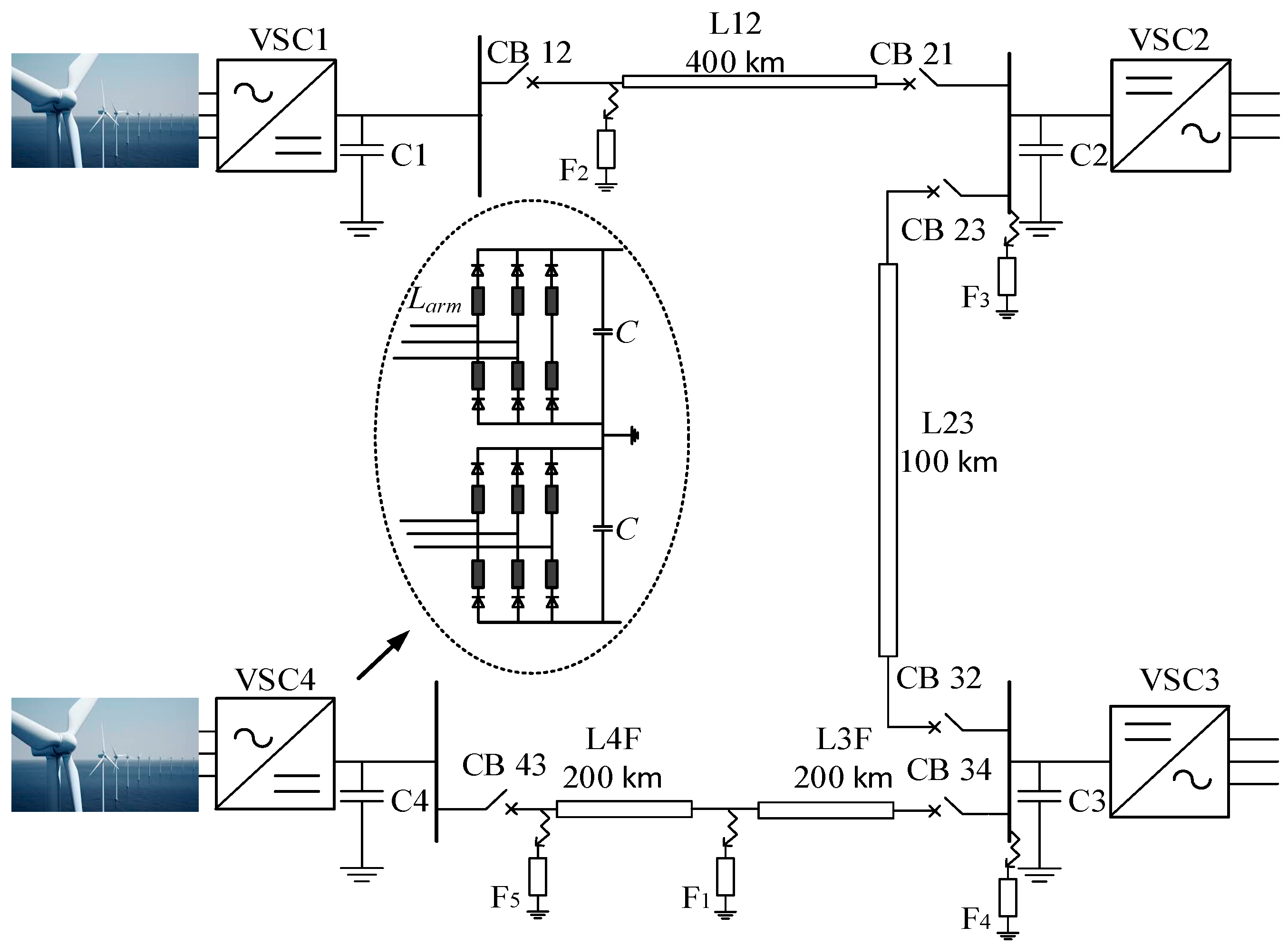
3.2. Converter and Network Model

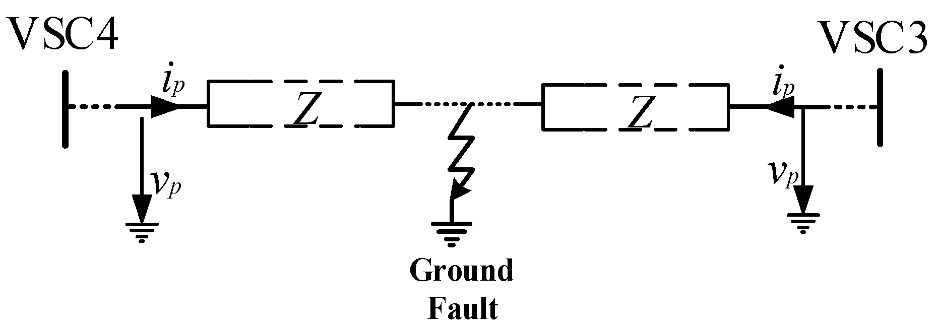
A four-terminal MTDC network is simulated in PSCAD and utilized properly during all circumstances as demonstrated in Figure 4. Terminal 1 and 4 are linked to wind farms that are placed in an offshore location. Terminal 2 and 3 are connected with the AC grid. The system voltage is 300 kV according to the initial conditions. A P–G fault is induced between Terminal 3 and 4 by performing simulation at the center of the cable. Numerous contributing sources are analyzed separately at the time of fault with the aim of designing the most suitable breaker schemes to minimalize the fault current. Additionally, the dependence of fault current and terminal voltage is critically analyzed with certain parameters. The converters are designed as ±300 kV bipolar half-bridge VSC configuration with DC link capacitors that are independently grounded at respective terminals. The parameters of the system are articulated in

Table 2. System parameters.

Parameters	Values
Rated converter power	1000 MW
Alternating current (AC) voltage (P–P, RMS)	500 kV
Direct current voltage	±300 kV
Reactance to resistance ratio of AC network	10
Transformer leakage reactance	0.1 p.u.
Total resistance of converter diodes	0.005 p.u.
Converter phase reactor	0.05 p.u.

P–P: pole to pole; RMS: root mean square value.

and the equivalent model of the VSC converter is shown in Figure 4.

4. Methodology

A P–G fault with a fault resistance of 0.01 Ω is simulated at the center of VSC3 and VSC4 in a base case. A propagation delay is considered as the signal transportation delay to evaluate the limited speed between two terminals of the transmission cable. In Figure 5, the propagation delay, T_p is induced between Terminal 3 and Terminal 4 of the cable having length 400 km. The methodology applied for the analysis of propagation delay is based on the forward and backward traveling waves.

The basic computations, based on traveling wave theory [18], for voltage V and current I at any point p of the cable, are carried out through partial differential equations, as expressed in Equations (4) and (5).

$$\frac{\partial v}{\partial p}=-\left(L\frac{\partial i}{\partial t}+Ri\right)$$

(4)

$$\frac{\partial i}{\partial p}=-\left(C\frac{\partial v}{\partial t}+Gi\right)$$

(5)

The factor R indicates the resistance per unit length and is responsible for voltage drop owing to the conductor’s ohmic losses, whereas, the parameter G signifies the conductivity per unit length at the constant voltage between conductors. The dual conductor model of the cable with losses can be solved using the Laplace domain:

$$-\left(\frac{dV}{dp}\right)=I\times Z\left(s\right)$$

(6)

$$-\left(\frac{dI}{dp}\right)=V\times Y\left(s\right)$$

(7)

The impedance and the admittance are the factors for the inductance and the capacitance respectively as explained by the equations as follows:

$$Z(s)=R+sL$$

(8)

$$Y(s)=G+sC$$

(9)

solving for the independent expression of the current and voltage to assess the parameters at any point in the cable, Equations (10) and (11) are obtained as:

$$\frac{d^{2}V}{d{p}^2}=-k^2(s)V=0$$

(10)

$$\frac{d^{2}I}{d{p}^2}=-k^2(s)I=0$$

(11)

Here, k(s) is the propagation constant and its value is given as follows:

$$k(s)=\sqrt{Y(s)\times Z(s)}$$

(12)

Afterward, the second order differential Equations (10) and (11) for current and voltages are expressed as:

$$V(p,s)=\left[V^{+}(s)e^{-k(s)p}+V^{-}(s)e^{k(s)p}\right]$$

(13)

$$I(p,s)=\frac{1}{Z^{\ast }(s)}\left[V^{+}(s)e^{-k(s)p}-V^{-}(s)e^{k(s)p}\right]$$

(14)

where $V^{+}(s)$ and $V^{-}(s)$ are the amplitude of the forward and backward traveling waves correspondingly and the value of Z*(s) is expressed as:

$$Z^{\ast }(s)=\sqrt{\frac{Z(s)}{Y(s)}}$$

(15)

Equations (13) and (14) are applicable to evaluate the basic parameters of a cable.

5. Proposed Model

The shunt parameters of conductance G and capacitance C are independent of the frequency, whereas the resistance divulges the maximum dependence on the frequency due to skin effect as expressed in Figure 6. The current travels on the surface of the conductor at high frequencies and commensurate with small penetration depths producing escalation in the effective resistance. The expressions for the current $i_p(x,y)$ and voltage $v_p(x,y)$ at any point p of the cable can be obtained in the time domain for analyzing the propagation delay. As mentioned previously, only the cable resistance is highly dependent on the frequency, whereas the remaining parameters are virtually constant and can be neglected in the thorough evaluation. The ground fault originates a negative voltage surge with an extremely steep waveform, which results in the production of high frequencies. The impedance and admittance of the cable can be expressed in the Laplace domain, as described in Equations (16) and (17):

$$Z\left(s\right)=K·\sqrt{s}+L·s$$

(16)

$$Y\left(s\right)=C·s$$

(17)

where K represents the skin effect, expending the propagation constant and characteristic impedance respectively.

$$k(s)=\sqrt{(K·\sqrt{s}+L·s)·C·s}$$

(18)

$$Z_0(s)=\sqrt{\frac{K·\sqrt{s}+L·s}{C·s}}$$

(19)

By applying binomial expansion on Equations (18) and (19), and truncating the higher terms for the approximate solution, the propagation speed at the higher frequencies can be calculated using the expression, $c=1/\sqrt{LC}$. However, the impedance of the cable characteristics can be determined using the relation, $R_0=\sqrt{L/C}$. As a result, a suitable solution is determined as expressed in Equations (20) and (21).

$$k(s)\approx \frac{s}{c}\left(1+\frac{K}{2L}·s^{-\raisebox{1ex}{$1$}\!\left/ \!\raisebox{-1ex}{$2$}\right.}\right){\displaystyle \sum _{i=1}^n{X}_i}$$

(20)

$$Z_0(s)\approx R_0\left(1+\frac{K}{2L}·s^{-\raisebox{1ex}{$1$}\!\left/ \!\raisebox{-1ex}{$2$}\right.}\right)$$

(21)

Equations (13) and (14) are used for the forward and backward traveling waves. However, by considering the forward traveling wave only and taking the initial voltage step of magnitude V₀ at the fault position. These equations lead to determine the solutions for the fundamental parameters in forward traveling waves as described in Equations (22) and (23):

$$V(p,s)=V^{+}(s)·e^{-k(s)p}$$

(22)

$$I(p,s)=\frac{1}{Z_0(s)}{V}^{+}(s)·e^{-k(s)p}$$

(23)

Using the inverse Laplace transform for determining the time domain solution [23].

$$v_p(x,t)=V_0·erfc\left(\frac{\partial }{2\sqrt{t-T}}·T\right)·u(t-T)$$

(24)

$$i_p(x,t)=\frac{V_0}{R_0}·e^{{\partial }^{2}t}·erfc\left(\frac{\partial }{2\sqrt{t-T}}·T+\partial \sqrt{t-T}\right)·u(t-T)$$

(25)

Equation (26) indicates the traveling wave delay.

$$T=\raisebox{1ex}{$x$}\!\left/ \!\raisebox{-1ex}{$c/n$}\right.$$

(26)

where $\partial =k/2L$ is the distortion factor, u(t) represents the unit step function, erfc is expressed as the complementary error function [24], x is the distance between the measuring points, c is the speed of light in vacuum and n signifies the reflection index of the optical fiber.

A reflection index was assumed to be 1.4682 for a SMF-28 ultra-optical fiber. The proposed expressions give an exact approximation for the analysis of propagation delay and evaluation of the current and voltage during the faults for high frequency surges. Hence, the approximate propagation delay of 400 km cable must be about 2 ms accordingly.

6. Results and Evaluation

In this section, the results for different cases of propagation time delay in MTDC network, depending on the distance between the terminals of transmission lines, are obtained in PSCAD and validated through RTDS. In case of a fault, a fault surge arises, which travels towards the relay measuring points with a short delay, known as propagation delay or transportation delay. A P–G fault in a four-terminal MTDC network is analyzed in the base case. Results are presented for the propagation delay to assist in designing the reliable protection schemes and investigating the performance of the system. The critical analysis of the results is carried out regarding different fault locations in a MTDC network in order to evaluate the fault current and terminal voltage.

6.1. Propagation Time Delay Testing for Cable

The illustration of propagation delay is an important aspect for designing the protection scheme of MTDC networks. The propagation delay in the MTDC network has been confirmed for the base case. A P–G fault F₁ is incepted at t = 1.0 s at the center of the cable between VSC3 and VSC4 on the cable having its total length of 400 km. The fault surge arrives after a certain time delay at each terminal according to the distance from the fault point. Voltages and fault currents across each terminal are taken into account in this study. T_f is the time of fault, which is expressed with a dotted line, and t₁ to t₄ represents the time delays for VSC1 to VSC4 respectively. Figure 7 depicts the propagation delay for voltages and currents. As it can be shown in Figure 7, prior to the occurrence of fault, the rated value of voltage is 300 kV. The fault occurs at t = 1.0 s, as represented with T_f. VSC3 (blue curve) and VSC4 (pink curve) are 200 km away from the fault point, and the voltage drops after a time delay of 1 ms time. Moreover, VSC2 (red curve) and VSC1 (black curve) are 300 km and 700 km from the fault point respectively, and the voltage drop for them are 1.5 ms and 3.5 ms accordingly. Fault current across the MTDC terminals can also be determined by the same phenomenon as that of voltage. The fault current rises with a steep at the time of fault at T_f, beyond which the current rises after the specific propagation delay according to the response of the voltage depending upon their distance from the fault location. The first steep peak is due to discharging of the capacitive elements, whereas remaining peaks are due to the contribution of fault currents from other terminals consequently. These peaks also authenticate propagation delay of the faults signals from different terminals to the fault point, which has been explained previously as a backward surge in Section 2.

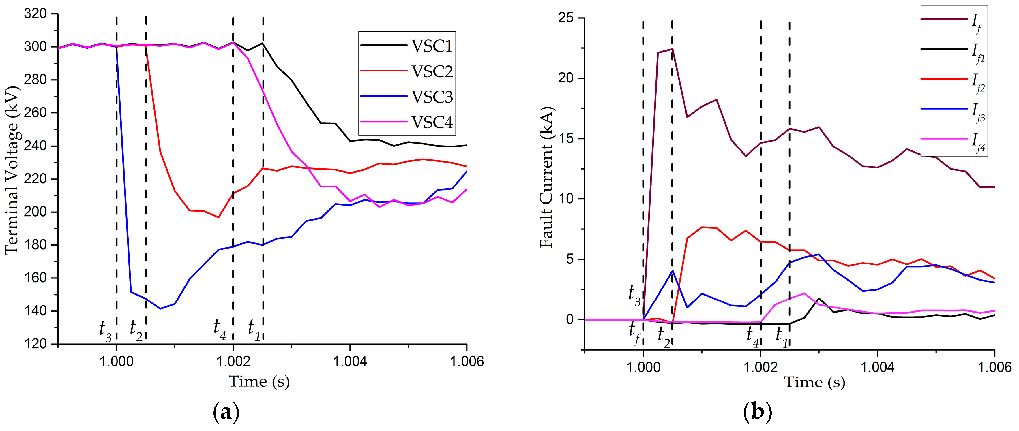
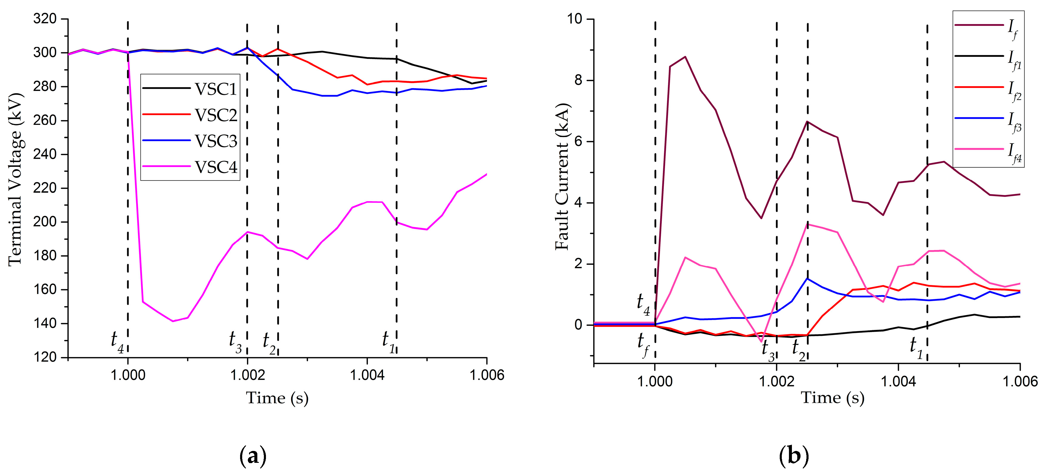
6.2. Different Cases for Propagation Time Delay

Different cases have been considered for evaluation of the proposed expressions, which are in exact approximation to the analysis of propagation delay. These considerations have been verified under different cases in MTDC network, with the inception of fault at multiple locations of the network. Fault cases are classified from F₂ to F₅ as depicted in Figure 4. The distance from fault location to different terminals of MTDC network and the prospective propagation delay is exhibited in

Table 3. Different fault scenarios.

Fault Type	Fault Location	Distance (km)	Propagation Delay (ms)
F2	F-T1	0	0
	F-T2	400	2
	F-T3	500	2.5
	F-T4	900	4.5
F3	F-T1	400	2
	F-T2	0	0
	F-T3	100	0.5
	F-T4	500	2.5
F4	F-T1	500	2.5
	F-T2	100	0.5
	F-T3	0	0
	F-T4	400	2
F5	F-T1	900	4.5
	F-T2	500	2.5
	F-T3	400	2
	F-T4	0	0

. The results for these cases are explained in Figure 8, Figure 9, Figure 10 and Figure 11.

Figure 8 expresses the response of voltages and fault currents during the fault F₂ which is incepted close to Terminal 1 as shown in Figure 4. The distances are calculated from the fault point to each terminal of the MTDC network as shown in Figure 8. However, before the occurrence of fault, the system is stable and a fault is incepted at t = 1.0 s as represented with T_f. The fault occurs at VSC1, with reciprocal changes in voltage and current, the voltage stoops down to the lowest level with simultaneous rise in the current. Afterward, the VSC2 (red curve) is 400 km away from the fault point, and the voltage drops after 2 ms time delay for them. Moreover, VSC3 (blue curve) and VSC4 (pink curve) are 500 km and 900 km from the fault point correspondingly, and the voltage drop for them are 2.5 ms and 4.5 ms respectively. Similarly, fault current can also be determined for the MTDC network by employing similar phenomenon. The calculated outputs in Table 3, using the proposed expressions, are in accordance with the results depicted in Figure 8. Likewise, Figure 9 expresses the results during the fault, F₃ which occurs close to the VSC2. The response shows that the voltage and current across the VSC2 (red curve) changes rapidly just after the occurrence of the fault. Moreover, the voltage drops on other terminals, with respect to the distance. Hence, the calculated output values using the proposed expressions are the same as the results presented in Figure 9. Correspondingly, the results of F₄ and F₅ are illustrated in Figure 10 and Figure 11 respectively, which have the same response as that calculated by the proposed expressions. Therefore, it is substantiated that the outputs of the proposed analytical expressions for propagation delay are in exact approximation with the simulated results at different fault locations.

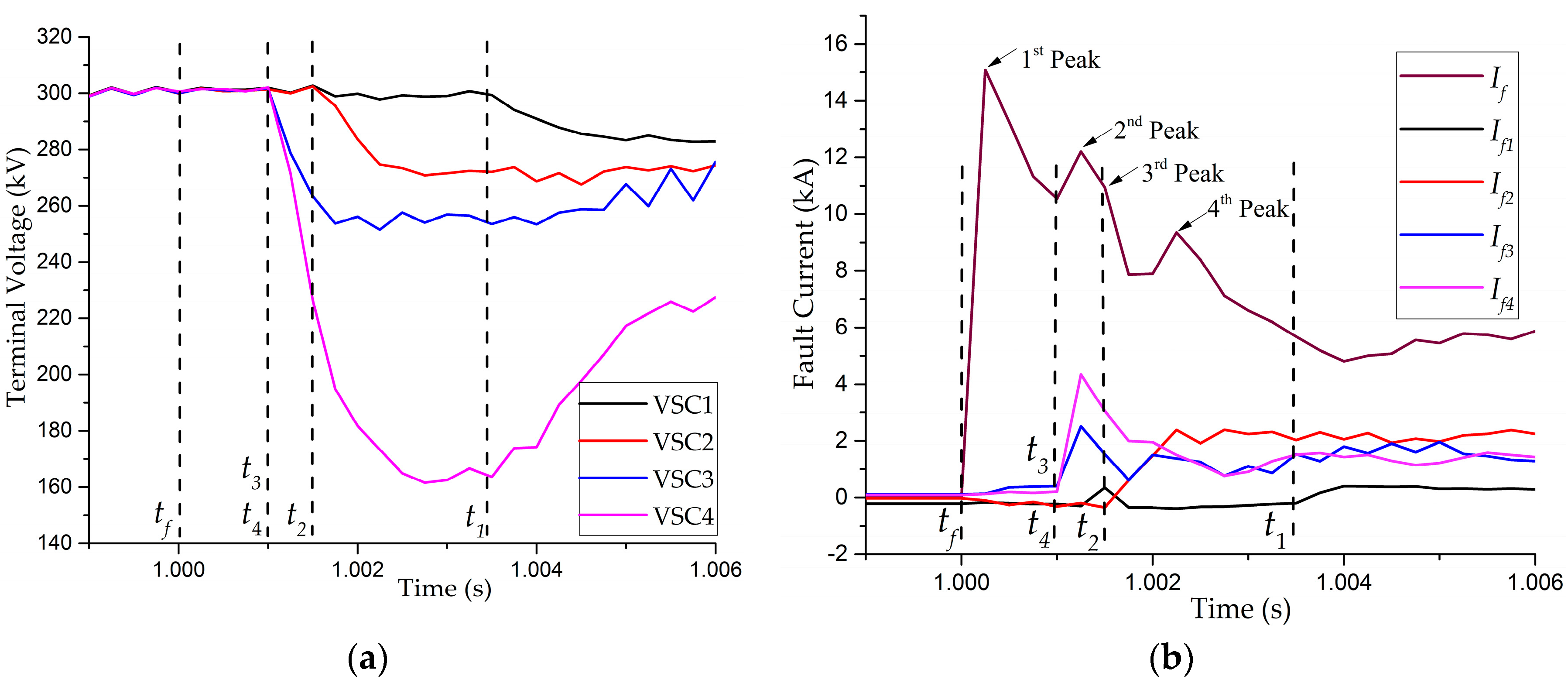
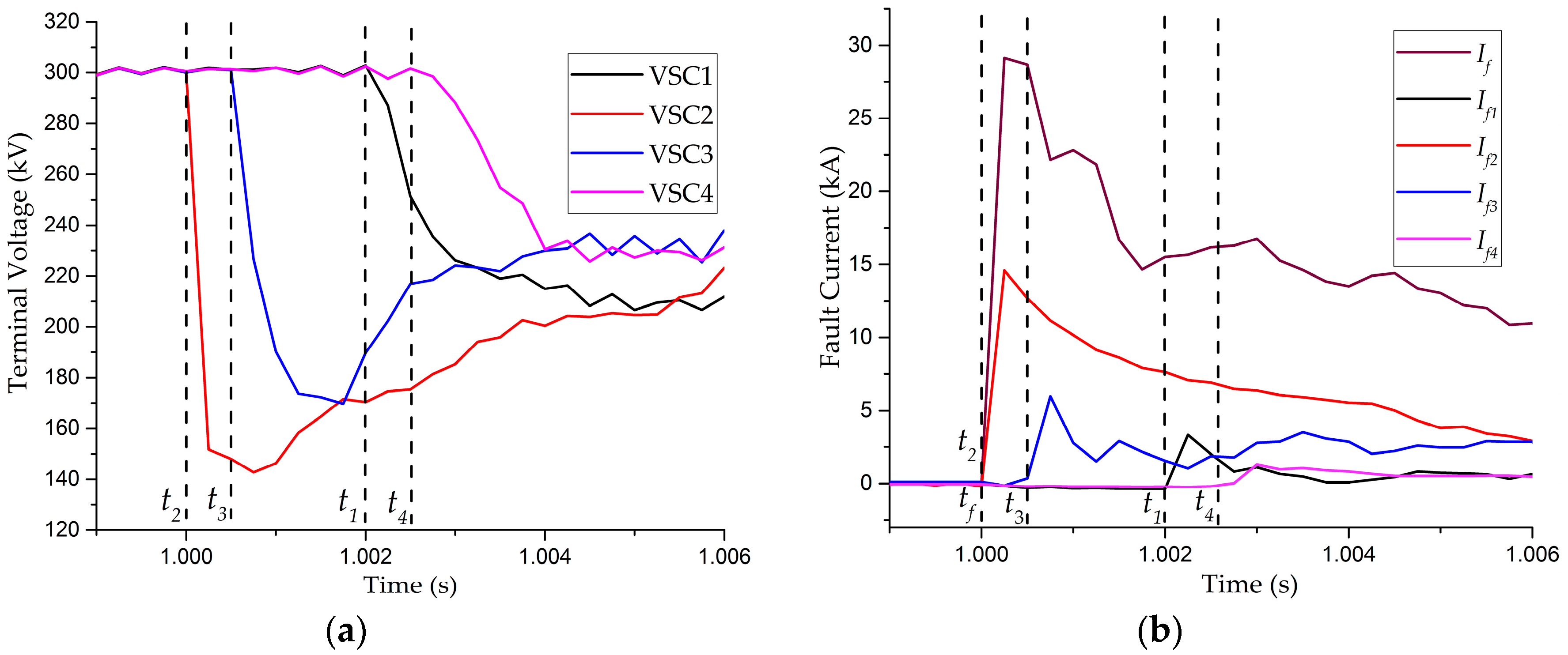
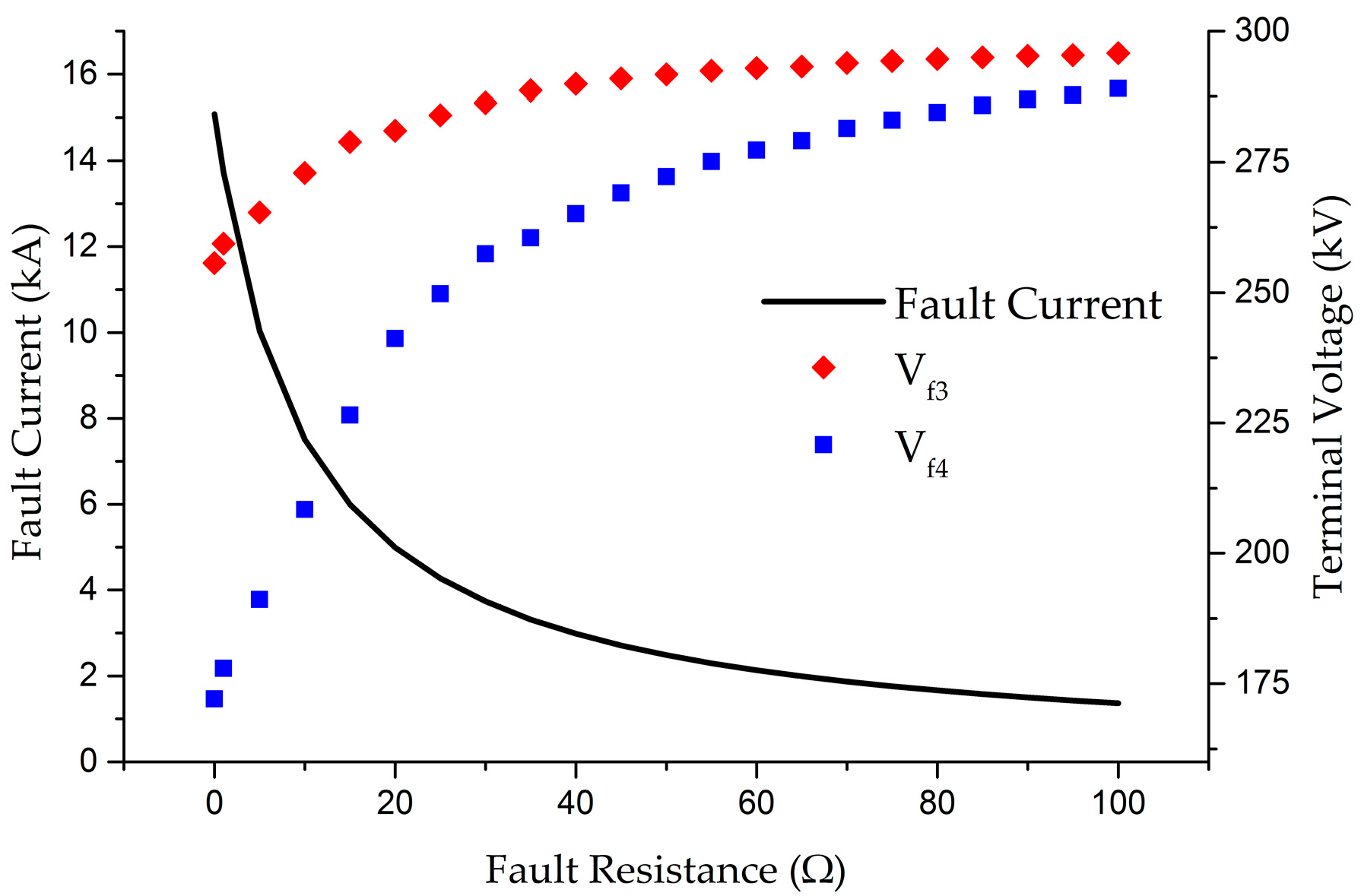
6.3. Terminal Voltage and Fault Current Dependence

Numerous simulations were performed to analyze the dependence of terminal voltage and fault current in the calculation of propagation delay. The results express the utmost dependence on the fault resistance. The value of the fault resistance increased from 0 Ω to 100 Ω for the base case and all other parameters stayed constant. The fault current gradually decreased up to 2 kA at higher value of the fault resistance as expressed in Figure 12 (black curve). Moreover, the voltage drop had its minimal values at the higher fault resistance values. The nearest terminal voltages were taken into account for the analysis of the dependence of the fault resistance, as can be seen with the lowest voltage drop at higher values of the fault resistance for VSC3 (red dots) and for VSC4 (blue dots) is exhibited in Figure 12.

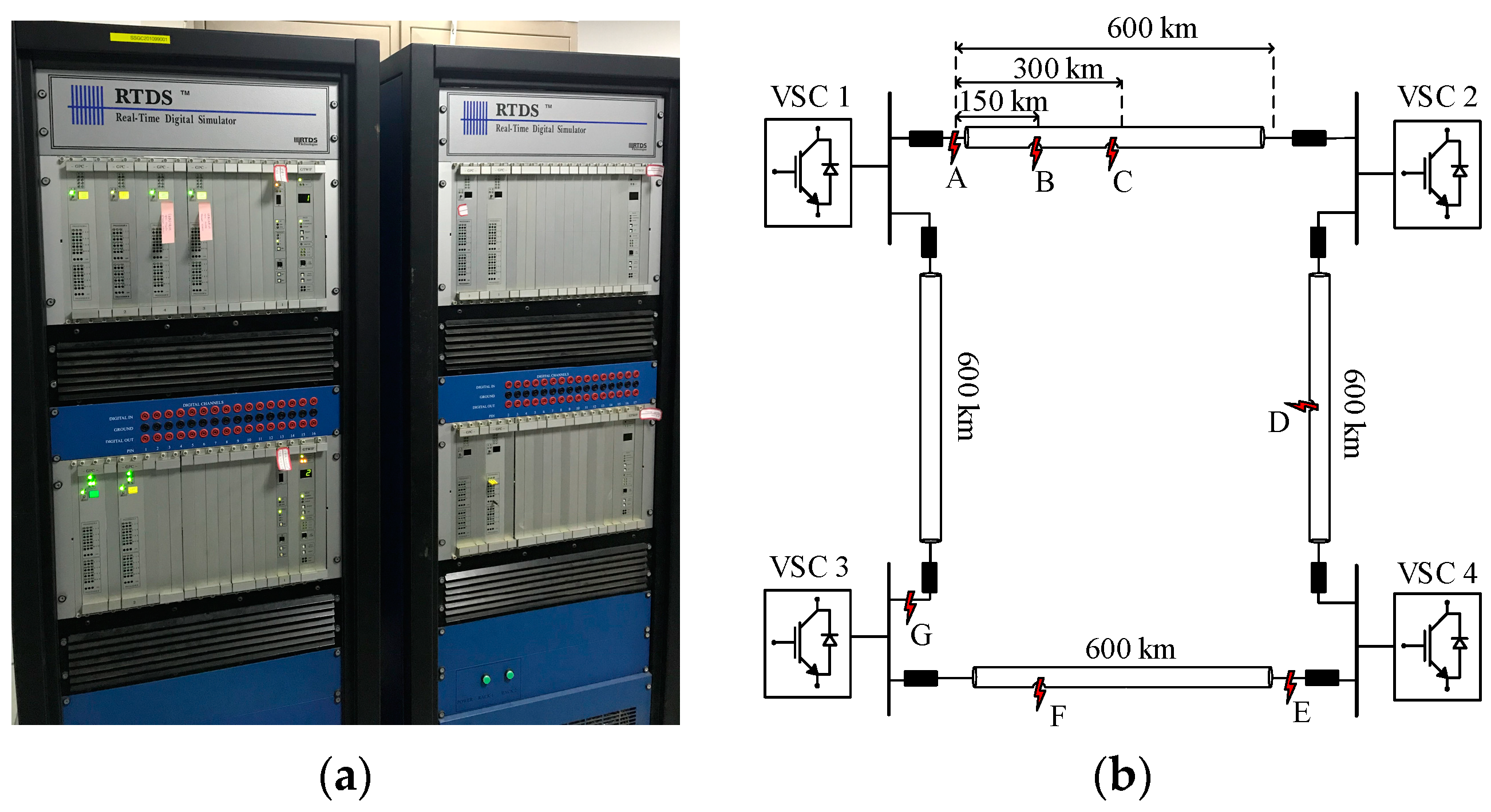
6.4. Validation of Propagation Delay with Real-Time Digital Simulator (RTDS)

MTDC networks are adequate solutions for the development of future HVDC grids. A ±400 kV four-terminal MTDC network for a VSC is constructed on the real-time digital simulator to investigate the adaptability of the proposed expression for propagation delay. Figure 13a expresses the system topology and real-time digital simulator (RTDS) module. Faults are incepted at different locations at t = 1.0 s, named as A to G, with the fault resistance of 0.01 Ω, as it can be seen in Figure 13b. The black spots represent the measuring points in the system. The voltage drop is measured for every fault at each measuring point and the results are tabulated in

Table 4. Performance of the proposed protection scheme.

Fault Name	Tvsc1 (CALC)	Tvsc1 (MEAS)	Tvsc2 (CALC)	Tvsc2 (MEAS)	Tvsc3 (CALC)	Tvsc3 (MEAS)	Tvsc4 (CALC)	Tvsc4 (MEAS)
A	1.00000	1.000000	1.00300	1.003001	1.00300	1.003001	1.0060	1.006012
B	1.00075	1.000754	1.00225	1.002248	1.00375	1.003748	1.00525	1.005261
C	1.00150	1.001496	1.00150	1.001503	1.00450	1.004500	1.00450	1.004495
D	1.00450	1.004504	1.00150	1.001497	1.00150	1.001501	1.00450	1.005453
E	1.00600	1.006007	1.00300	1.003000	1.00300	1.003007	1.00000	1.000000
F	1.00375	1.003745	1.00525	1.005298	1.00075	1.000749	1.00225	1.002248
G	1.00300	1.003002	1.00600	1.006003	1.00000	1.00000	1.00600	1.006012

. Meanwhile, the propagation of the signals is also calculated with the proposed expressions which are listed in Table 4. The results illustrate that the proposed expressions are found accurate for calculating the propagation delay, and that this method can be utilized for proposing the protection schemes of future MTDC networks.

7. Conclusions

This paper contributes in assessing the propagation delay in multi-terminal high voltage DC networks during faulty conditions. The propagation delay is analyzed through analytical approximation in the time domain by taking only the forward traveling wave into account and considering the initial voltage step of magnitude at the fault position. These analytical formulas prove to be propitious for the evaluation of propagation delay in transmission lines, with consideration of fault resistance and its effect on basic system parameters during calculations. The proposed scheme is corroborated through detailed simulations in PSCAD for different parameters and arrangements to explore the proposed model. Furthermore, RTDS validated that the proposed approach is promising for the evaluation of propagation delay in large MTDC networks. Additionally, this method solves the discrepancy of assuming random values of propagation delay, as presumed previously by various researchers while proposing their respective protection schemes; however, the proposed expression calculates a standard value of 200 km/ms as propagation delay. In general, good accuracy is achieved with negligible errors below 0.3% and the proposed scheme enables a simple and highly accurate representation of the temporal development of initial voltage step without detailed simulations, even for very complex curves with multiple surges. These calculations may serve as a benchmark for future MTDC network standard calculations.

References

1. Yaramasu, V.; Wu, B.; Sen, P.C.; Kouro, S.; Narimani, M. High-power wind energy conversion systems: State-of-the-art and emerging technologies. Proc. IEEE 2015, 103, 740–788. [Google Scholar] [CrossRef]
2. Zervos, A.; Kjaer, C. Pure Power: Wind Energy Targets for 2020 and 2030. Available online: http://www.ewea.org/ (accessed on 20 May 2018).
3. De Decker, J.; Kreutzkamp, P. OffshoreGrid: Offshore Electricity Infrastructure in Europe. 2011. Available online: http://www.offshoregrid.eu/ (accessed on 8 June 2018).
4. The North Seas Countries’ Offshore Grid Initiative. NSCOGI 2013/2014 Progress Report. Available online: http://www.benelux.int/files/9814/0922/7026/NSCOGI_2013_2014.pdf (accessed on 8 August 2017).
5. Hertem, D.V.; Ghandhari, M. Multi-terminal VSC HVDC for the European super grid: Obstacles. Renew. Sustain. Energy Rev. 2010, 14, 3156–3163. [Google Scholar] [CrossRef]
6. Negra, N.B.; Todorovic, J.; Ackermann, T. Loss evaluation of HVAC and HVDC transmission solutions for large offshore wind farms. Electr. Power Syst. Res. 2006, 76, 916–927. [Google Scholar] [CrossRef]
7. Flourentzou, N.; Agelidis, V.; Demetriades, G. VSC-based HVDC power transmission systems: An overview. IEEE Trans. Power Electron. 2009, 24, 592–602. [Google Scholar] [CrossRef]
8. Liu, C.C.; He, L.; Finney, S.; Adam, G.P.; Curis, J.B.; Despouys, O.; Prevost, T.; Moreira, C.; Phulpin, Y.; Silva, B. Preliminary Analysis of HVDC Networks for Off-Shore Wind Farms and Their Coordinated Protection; Technical Report for Status Report for European Commission; European Commission: Brussels, Belgium; Luxembourg, 2011. [Google Scholar]
9. Hajian, M.; Zhang, L.; Jovcic, D. DC transmission grid with low-speed protection using mechanical DC circuit breakers. IEEE Trans. Power Deliv. 2015, 30, 1383–1391. [Google Scholar] [CrossRef]
10. Sanusi, W.; Hosani, M.A.; Moursi, M.S.E. A novel DC fault ride-through scheme for MTDC networks connecting large-scale wind parks. IEEE Trans. Sustain. Energy 2017, 8, 1086–1095. [Google Scholar] [CrossRef]
11. Tzelepis, D.; Dyśko, A.; Fusiek, G.; Nelson, J.; Niewczas, P.; Vozikis, D.; Orr, P.; Gordon, N.; Booth, C.D. Single-ended differential protection in MTDC networks using optical sensors. IEEE Trans. Power Deliv. 2017, 32, 1605–1615. [Google Scholar] [CrossRef]
12. Nadeem, M.H.; Tai, N.; Zheng, X.; Gul, M. Multi-Terminal HVDC Fault Current Analysis During Line to Ground Fault. In Proceedings of the IEEE Innovative Smart Grid Technologies IGST Asia 2017, Auckland, New Zealand, 1–5 December 2017. [Google Scholar]
13. Nadeem, M.H.; Zheng, X.; Tai, N.; Gul, M.; Baloch, M.H. Analysis of Fault Current Contribution and Impact of Key Parameters in MTDC Network. Interciencia J. 2017, 42, 257–268. [Google Scholar]
14. Nadeem, M.H.; Zheng, X.; Tai, N.; Gul, M. Identification and Isolation of Faults in Multi-terminal High Voltage DC Networks with Hybrid Circuit Breakers. Energies 2018, 11, 1086. [Google Scholar] [CrossRef]
15. Nadeem, M.H.; Zheng, X.; Tai, N.; Gul, M. Detection and Classification of Faults in MTDC Networks. In Proceedings of the IEEE PES Asia-Pacific Power and Energy Engineering Conference 2018, Sabah, Malaysia, 7–10 October 2018. [Google Scholar]
16. Abu-Elanien, A.E.B.; Abdel-Khalik, A.S.; Massoud, A.M.; Ahmed, S. A non-communication based protection algorithm for multi-terminal HVDC grids. Electr. Power Syst. Res. 2017, 144, 41–51. [Google Scholar] [CrossRef]
17. Wang, J.; Liew, A.C.; Darveniza, M. Extension of dynamic model of impulse behavior of concentrated grounds at high currents. IEEE Trans. Power Deliv. 2015, 20, 2160–2165. [Google Scholar] [CrossRef]
18. Miano, G.; Antonio, M. Transmission Lines and Lumped Circuits: Fundamentals and Applications; Academic Press: San Diego, CA, USA, 2001; Available online: https://www.elsevier.com/books/transmission-lines-and-lumped-circuits/miano/978-0-12-189710-9 (accessed on 25 March 2018).
19. Bucher, M.K.; Franck, C.M. Contribution of fault current sources in multiterminal HVDC cable networks. IEEE Trans. Power Deliv. 2013, 28, 1796–1803. [Google Scholar] [CrossRef]
20. Worzyk, T. Submarine Power Cables: Design, Installation, Repair, Environmental Aspects; Springer Science & Business Media: Berlin, Germany, 2009. [Google Scholar]
21. Mura, F.; Christoph, M.; Doncker, R.W.D. Stability analysis of high-power dc grids. IEEE Trans. Ind. Appl. 2010, 46, 584–592. [Google Scholar] [CrossRef]
22. Dodds, S. HVDC VSC (HVDC Light) Transmission—Operating Experiences; CIGRE: Paris, France, 2010. [Google Scholar]
23. Magnusson, P. Transient wavefronts on lossy transmission lines—Effect of source resistance. IEEE Trans. Circuit Theory 1968, 15, 290–292. [Google Scholar] [CrossRef]
24. Abramowitz, M.; Stegun, I.A. Handbook of Mathematical Functions: With Formulas, Graphs, and Mathematical Tables; US Government Printing Office: Washington, DC, USA, 1964.
Figure 1. Reflection coefficient: (a) Right after the fault occurrence and negative voltage surge travels towards terminals, (b) Backward traveling surge, divides into transmission and reflection coefficient.
Energies 11 02115 g001
Figure 2. Function of fault current and the reflection coefficient at the fault point.
Energies 11 02115 g002
Figure 3. Cable cross-sectional layout model.
Energies 11 02115 g003
Figure 4. Multi-terminal high voltage direct current network layout indicating voltage-source converter (VSC)-based converter topology.
Energies 11 02115 g004
Figure 5. Propagation delay between the two ends of cable.
Energies 11 02115 g005
Figure 6. Discharge of ground fault.
Energies 11 02115 g006
Figure 7. Propagation time delay in MTDC (multi-terminal high voltage direct current) network. (a) Voltage response, (b) current response.
Energies 11 02115 g007
Figure 8. Propagation time delay in MTDC network in case of fault near VSC1. (a) Voltage response, (b) current response.
Energies 11 02115 g008
Figure 9. Propagation time delay in MTDC network in case of fault near VSC2. (a) Voltage response, (b) current response.
Energies 11 02115 g009
Figure 10. Propagation time delay in MTDC network in case of fault near VSC3. (a) Voltage response, (b) current response.
Energies 11 02115 g010
Figure 11. Propagation time delay in MTDC network in case of fault near VSC4. (a) Voltage response, (b) current response.
Energies 11 02115 g011
Figure 12. Effects of fault resistance on fault current and the surrounding terminal voltage.
Energies 11 02115 g012
Figure 13. Real-time digital simulator (RTDS) device and VSC-MTDC network for the validation of propagation delay (a) RTDS device, (b) Four-terminal VSC-MTDC network.
Energies 11 02115 g013