A Numerical Investigation of Frost Growth on Cold Surfaces Based on the Lattice Boltzmann Method

1
MOE Key Laboratory of Thermo-Fluid Science and Engineering, School of Energy and Power Engineering, Xi’an Jiaotong University, Xi’an 710049, China
2
School of Mechatronic Engineering, Xi’an Technological University, Xi’an 710021, China
3
Department of Thermal Power Engineering, School of Energy and Power Engineering, Xi’an Jiaotong University, Xi’an 710049, China
*
Author to whom correspondence should be addressed.
Energies 2018, 11(8), 2077; https://doi.org/10.3390/en11082077
Submission received: 17 July 2018
/
Revised: 4 August 2018
/
Accepted: 7 August 2018
/
Published: 9 August 2018
Abstract
:A numerical investigation of frost growth on a cold flat surface was presented based on two-dimensional Lattice Boltzmann model. This model has been validated to have less prediction error by past experiments. According to the results, it is shown that average frost density appears different at an increasing rate at different frosting stages. In addition, cold surface temperature has great influence on frost growth parameters such as frost crystal deposition mass, frost deposition rate, and frost crystal volume fraction. It was found that the frost crystal deposition mass, frost crystal volume, and the deposition rate first increase rapidly, then gradually slow down, finally remaining unchanged while the cold surface temperature decreases. The further away from the cold surface, the more sparser the frost layer structure becomes due to the smaller frost crystal volume fraction.
1. Introduction
Heat exchangers will be subjected to deposition and progressive growth of frost, when humid air flows through the heat exchangers’ surface where the temperature is less than both zero degrees centigrade and the ambient air dew point temperature. Because of the frost layer insulation and its blockage of airflow, frosting will bring about the reduction of a heat exchanger’s performance and a greater pressure drop. In addition, unavoidable defrosting has to consume extra energy. Therefore, to guarantee normal operation of the heat exchanger, a frosting investigation on a cold surface is necessary. Apart from previous experimental studies [1,2,3], theoretical studies on frost growth predictions have been paying more attention.
A lot of predictions of frost growth have been carried out. In 1984, a molecules diffusion model was proposed by O’Neal et al. [4]. In their model, the frost layer was regarded as a porous media and the mass transfer in the frost formation process not only increases frost thickness but also increases frost density simultaneously. Later, this model was continually simplified and improved by researchers [5,6,7].
Tao et al. [8] assumed the frost a homogeneous porous medium and proposed a model to simulate the fully developed frost growth defined by Hayashi et al. [9]. Lee et al. [10] assumed humid air at the frost surface as a saturated state and developed a one-dimensional model considering water vapor molecular diffusion. Different from previous theoretical models with the assumption of saturated humid air, a new model within the threshold (15%) was established by Webb et al. [11] to predict frost deposition and growth. According their work, the air at the frost surface was confirmed to be in supersaturated state. Hermes et al. [12] formulated a mathematical model within ±10% error bands. In their model, they considered the air to be in a supersaturated state and regarded the frost as a porous media. In another study, a one-dimensional frost growth model was developed by Kandula [13] based on Jones and Parker [14] and Cheng et al. [15]. New frost correlations for density and effective thermal conductivity on a flat plate were formulated in Kandula’s study. Depending on semi-empirical correlations, Loyola et al. [16] presented a one-dimensional model to simulate the frost formation on parallel-plate channels under the conditions of the supersaturated humid air near the frost surface. All these above listed studies are one-dimension models simulating frost growth, assuming the frost layer to be a homogeneous porous media. These models mainly depend on empirical correlations to calculate frost parameters such as density and effective thermal conductivity and so on. Furthermore, some two-dimensional models were established to study frost growth without using frost empirical correlations in recent years. Lüer et al. [17] developed a two-dimensional transient model to study frost formation between parallel plate channels based on the conservation laws of mass, energy, and momentum. Their numerical results show good agreement with their experimental findings. With this model, local temperature and porosity of frost layer can be provided. Armengol et al. [18] also presented a two-dimensional model for frost growth over parallel plates adopting the finite volume method. The predicted frost thickness shows agreement with experimental data within a 10% error. Without adopting any experimental correlations, Lee et al. [6] established a transient two-dimensional prediction of frost deposition on a cold flat surface with agreement of about 10%. Another two-dimensional model was also proposed by Lenic et al. with initial frost density of 30 kg/m3 and initial frost thickness of 0.02 mm [19]. In his model, the moist air was assumed to be in a super-saturated state. Some CFD models were also adopted to simulate frost formation within acceptable deviation [20,21,22]. More recently, Negrelli et al. [23] investigated the frost effective thermal conductivity in details based on fractal theory with an approximately ±15% uncertain threshold compared to experimental results. Although the above models show good tendency with experimental points, the deviations in most models are about 10%. Therefore, better accurate prediction is needed.
The lattice-Boltzmann (LB) method is a novel numerical method. Compared with the traditional simulation methods, the LB model has attracted wide attention for its adaptability to complex structures and has achieved success in some areas, such as porous media and multiphase [24]. Manz et al. [25] conducted experiments and numerical simulations of randomly stacked porous bodies and found that the results of the LB simulation agree well with the experimental data, demonstrating the suitability of LB for simulating flow in porous media. Tang et al. [26] proposed a simplified analytical model for micro-scale porous media, and used the LB model to simulate the flow field of micro-scale porous media. Li et al. [27] proceeded from the lattice-Boltzmann collision model to realize the numerical simulation of the fluid migration process in dual porous media. Xu et al. [28] adopted a regular hexagonal model (FHP-7Bit model). They also established a corresponding seepage numerical model according to the relevant LB theory. This model was verified to be accurate. Wang et al. [29] used the LB model to simulate the process of gas seepage in dense porous media. The correctness of the simulation results was verified. With this approach, the flow field in the porous medium in the seepage flow was obtained. All the above studies show that the LB model is feasible and suitable to simulate the flow and heat transfer phenomenon in porous media. As mentioned above, it is known that the frost layer, consisting of a great number of frost crystals, acts as a porous media [4]. We have been trying to use the LB model to predict frost growth in recent years. We established a LB model to simulate the solidification process of water droplets effectively. Furthermore, we have also adopted this LB model to investigate frost growth and have acquired some preliminary findings [30]. In order to obtain more detailed information on frost growth, we will continue our study deeply following our previous LB model.
This study presents a two-dimensional LB model to simulate the frost growth on a cold flat surface based on the fractal theory (DLA model). In this model, the frost layer was regarded as a heterogeneous medium and the humid air near the frost surface is considered to be in actual super-saturation state. Compared to experimental data, the simulation results show good agreement; the maximum relative error is 8.05%. According to this model, the dynamic variation rules of frost layer properties have been investigated thoroughly.
The frost layer growth model based on the LB method has a good agreement with the experimental results. The model can be used to predict the growth of the frost layer and explain the characteristics of each stage of frost layer growth. It can provide more detailed information about frosting on flat cold surfaces. Meanwhile, it can also help to find reasonable defrost strategies and to optimize heat exchanger design under frosting conditions. In the following research, this study will provide necessary information for frosting issues on complex cold, instead of flat cold, surfaces.
2. Numerical Model and Theory
This simulation was carried out based on the following hypothesis: (1) for the nucleation process of frost crystals, homogeneous nucleation is adopted; (2) the crystal nucleus with a critical size formed by the water vapor condensation directly deposited on the existing frost crystals; (3) the humid air is considered as an incompressible Newton fluid; (4) in the simulation process, super-saturation and the relative humidity of humid air are assumed to be fixed; (5) during the frost growth, the melting and sublimation of frost crystals in some areas were neglected.
In order to create frost porous structure, the fractal theory (DLA model) is adopted in this two-dimensional LB model. According to DLA model, a certain number of seed particles are randomly generated on the cold surface (X-axis) firstly. Then, in order to simulate the frost crystal after the phase transition nucleus of water vapor, a certain number of random particles are generated in the calculation region using a random function; the probability of random particles generated is related to the freezing probability in Equation (1). The distance between random particles and seed particles is firstly calculated, and random particles will attach to the main frost crystal at the seed position with the smallest distance. In this way, the random particles generated at the frost top layer calculation area will preferentially attach to the main frost trunk, which is the strong longitudinal growth characteristics. At the same time, in order to simulate the water vapor bypasses around the main frost crystals and condenses at the inside of the frost layer, random particles are also generated inside the frost layer and move towards downward, left, and right directions with equal probability. Then these random particles will attach to the nearest cold surface or existing frost crystals.
2.1. The Mass of Frost Layer
Based on the nucleation theory, the increase of frost crystal mass within the controlled volume per unit time is calculated by the following Equation [31]:
where the critical radius of the nucleus is:
where is the interface energy, is the water vapor saturation ratio, is the super-saturation degree of humid air. The nucleation rate is:
where is the Boltzmann constant. Based on the assumption of homogeneous nucleation, the contact angle is 180°. The kinetic constant of nucleation rate is:
where kg is the water molecular mass. The non-isothermal correction factor is:
In Equation (1), is the freezing probability, . is the frost crystal volume fraction. Based on the frost crystal volume fraction , the parameter [32] is written as . The diffusion resistance factors , and are equal to 0.58, 3, and 10, respectively. The frost crystal volume fraction is written as .
The equivalent density of frost layer is defined as . is porosity which refers to the volume fraction of voids between particles in a porous structure.
2.2. The Velocity Field and the Temperature Field in LB Model
In this LB model, the Bhatnagar–Gross–Krook (BGK) [33,34] approximation with two dimensions and nine velocities was adopted. For the velocity field, the distribution function is:
where is the velocity distribution function. and are the position of the particle and time, respectively. is the dimensionless relaxation time which is connected with the kinematic viscosity . The discrete velocity is:
where and are the lattice spacing and the time step, respectively. The equilibrium distribution function of velocity field is:
where is the isothermal sound velocity. The weight coefficients are .
The macroscopic density ρ and velocity u are defined as:
where v is an auxiliary velocity with two parameters and . is the geometric function and [35] is the permeability, is the diameter of the solid particle.
For the temperature field, the distribution function is:
where the dimensionless relaxation time is connected with the thermal diffusivity . The discretized source term is . The equilibrium distribution function of temperature field is:
The macroscopic temperature is:
where the heat capacity ratio [36] reflects the influence of the porous medium on the temperature field. and are the solid and fluid densities, and are the solid and fluid specific heats at the constant pressure.
The evolution of LB model mainly includes two processes: migration and collision.
- Migration:
- Collision:
During the process of evolution, temperature will be transferred into the system through the migration of particles on the boundary. And particle collision will occur due to the change of temperature. Therefore, migration process is regarded to happen before collision in this model.
2.3. Initial and Boundary Condition
The initial condition. The initial velocity of the velocity entrance boundary is equal to the air velocity, and the other nodes are zero. The initial temperature of cold wall is equal to the cold surface temperature, and the other nodes are equal to the air temperature.
The boundary condition. In the rectangular calculation area, the macroscopic temperature and velocity on the corresponding boundary were set as following. The velocity of left boundary is constant and equal to the inlet air velocity, and the temperature is equal to the humid air temperature. The velocity and temperature of the nodes on the right boundary and the top boundary are determined by the nearby front layer nodes by the non-equilibrium extrapolation format in the calculation process. The velocity of the bottom boundary (cold surface) is zero and the temperature is constant and equal to the cold surface temperature.
In the LB model, the velocity and temperature of the boundary nodes in each direction are determined by the distribution functions. Based on the macroscopic parameters of the boundary, the boundary conditions of the corresponding nodes are obtained. The details are as follows. For the cold wall nodes, the bounce-back format was adopted. A detailed schematic is shown in Figure 1a, and the distribution function of the boundary node is:
For the other three boundary nodes, the non-equilibrium extrapolation format was adopted. A detailed schematic is shown in Figure 1b, the nodes E, O, and A are located on the boundary, the nodes B, C, and D are located in the flow field, the nodes F, G, and H are located outside the flow field. The distribution function of the boundary node O is calculated in the following Equations:
2.4. Procedure of Numerical Model
Figure 2 shows the calculation flowchart.
In the simulation process, the initial physical parameters were firstly determined. The physical parameters include humidity, velocity, temperature and density of the humid air, cold surface temperature, relaxation time, lattice space, and boundary conditions. At the same time, a certain number of random nuclei were distributed on the cold wall nodes. Then the particles representing the frost crystal after the phase transition nucleus of water vapor, are randomly generated at the top of the calculation area and these particles move towards the left, right, and bottom directions with equal probability until they contact with the solid nodes. According to the frost crystal volume fraction, the number of crystals can be calculated. The initial velocity and temperature distribution functions are determined by and , respectively. Based on the Equation (1), the mass increase of the frost layer can be calculated. At the same time, the frost crystal volume fraction will be updated. Finally, based on the boundary conditions, the velocity and temperature distribution functions, as well as the macroscopic parameters, such as density, velocity and temperature, can be obtained.
2.5. Validation of LB Model
Figure 3 shows the comparison of the model results with the experimental data provided by a previous paper [19]. In Figure 3, air temperature Ta = 19.8 °C, air relative humidity = 58.0%, air velocity = 0.6 m/s, and cold surface temperature Tw = −20.5 °C. It can be seen from Figure 3 that the simulation results are in good agreement with the experimental data and that the maximum relative error is 8.05%.
3. Results and Discussion
Here, a domain of 4 mm × 3 mm is used, and the lattice number adopts 800 × 600. The following simulated air conditions are set as followings: Ta = 10.8 °C, = 41.2%, and = 0.16 m/s.
3.1. Frost Density
Figure 4 shows the variation of average density of frost layer over time. The cold surface temperature Tw = −16.5 °C. Generally speaking, the average density of frost layer increases with time. However, it can be seen that frost average density shows a different increasing rate at different frosting stages. In the incipient frosting, the curve has a little concave tendency. It is known that the frost exhibits strong dendritic growth during this early stage of frosting. That means the water vapor from the humid air mainly contributes to increase frost thickness while the rest proportion of water vapor increases and the density decreases. Therefore, the frost density growth slows down in the early stage of frosting. As the frost crystals continue to grow, the water vapor molecules continue to diffuse and desublimate to form nucleation deposits inside the frost layer. Therefore, the average density of frost increases gradually over time. However, due to the rise of the frost crystal surface temperature at the later stage of the frost growth, the freezing probability of the crystal nuclei decreases. As a result, the increase of the frost layer average density in the later stage is slower.
3.2. Frost Thickness
Figure 5 shows that the frost thickness changes with time under different cold surface temperatures. The cold surface temperature Tw are set as: 4.0 °C, −8.0 °C, −12.0 °C, and −16.0 °C. It can be seen that the frost thickness increases with the decrease of cold surface temperature and that the lower the cold surface temperature is, the greater the frost thickness increases. The main reason is that the water vapor will undergo the phase transition and form the crystal nucleus when the humid air approached the cold surface. Therefore, there will be a water vapor concentration gradient near the cold surface, which can force water vapor to move toward the cold surface. The lower the cold surface temperature, the greater the driving force due to the concentration gradient. It means that more water vapor molecules are able to contact and deposit on the cold surface or the existing frost crystal. Consequently, frost grows dramatically faster with the decrease of cold surface temperature.
3.3. Frost Deposition
The quantitative variation of frost crystal deposition can be used to measure the frost growth speed. Figure 6 and Figure 7 show the effect of cold surface temperature on the frost crystal deposition and the frost crystal deposition rate.
Figure 6 shows the evolution of frost crystal deposition per unit area over time at different cold surface temperatures. The cold surface temperature Tw are set as: −5.0 °C, −10.0 °C, −15.0 °C, and −20.0 °C. It can be observed that as the temperature of the cold surface decreases, the frost growth rate tends to increase, and the mass of the frost crystals increases significantly.
Figure 7 shows the evolution of frost crystal deposition rate with time. The cold surface temperature Tw are set as: −5.0 °C, −10.0 °C, −15.0 °C, and −20.0 °C. At first sight, the cold surface temperature has a prominent effect on frost crystal deposition rate. The frost crystal deposition rate increases dramatically with cold surface temperature decreasing. Besides, it can also be found that the frost crystal deposition rate increases with time and finally tends to remain unchanged. During the early frosting period, the increase in the frost crystal deposition rate is very rapid and occurs in a short time. This is due to the fact that in the early frost period, the crystals continue to grow upward in a dendritic form. Such dendritic structure acts as fins enhancing the effect of heat transfer and increasing the probability of phase transition. As a result, the frost crystals deposit faster. At the later frosting period, the water vapor hardly diffuses into the interior of the frost layer due to the increase of the frost surface temperature. Such a diffusion opportunity lessens with frost developing. Therefore, it is reflected that the deposition rate of frost crystals slows down gradually and approaches a constant value. Therefore, the deposition rate of the frost crystal is slowed down.
3.4. Frost Crystal Volume Fraction
Frost crystal volume fraction is the volume percentage of the frost crystal in the frosted area. It directly reflects the number of frost crystals and the density of the frost layer. At the same time, it can also reflect the porosity of the frost structure.
Figure 8 shows the distribution of the frost crystal volume fraction versus different frost thickness under different cold surface temperatures. The cold surface temperature Tw are set as: −5.0 °C, −10.0 °C, −15.0 °C, and −20.0 °C. It can be observed the frost crystal volume fraction distributes non-uniformly within the frost layer. The closer to the cold surface, the larger the frost crystal volume fraction, the more concentrated the frost crystal, and the larger the frost structure density. The further away from the cold surface, the smaller the frost crystal volume fraction, and the more sparse the frost crystal distribution. As the frost thickness increases, the volume fraction gradually decreases. This is due to the fact that water vapor diffuses from the outside to the inside of the frost layer and finally deposits at the bottom of the frost layer. So the more upwards along the frost thickness direction, the more sparsely the distribution of frost crystal is. At the same frost thickness, the lower the cold surface temperature, the frost crystal volume fraction is larger.
4. Conclusions
This paper presented a two-dimensional LB model to simulate frosting process on a cold surface based on the fractal theory (DLA model). This model was validated by experimental data with greater accuracy. According to the model, the dynamic variation rules of frost properties have been studied in detail. Some conclusions have been drawn out.
- (1)
- Frost average density shows different increasing rates at different frosting stages. The increase in the frost layer average density in the later frost growth stage is slower due to the rise of frost surface temperature.
- (2)
- Due to the effect of the cold surface temperature on the water vapor concentration gradient, the frost thickness increases dramatically with the decrease in the cold surface temperature.
- (3)
- The frost crystal deposition mass and deposition rate are greatly affected by the cold surface temperature. With the decrease in the cold surface temperature, the frost crystal deposition mass increase rapidly, and the deposition rate first increases rapidly, then gradually slows down, finally remaining unchanged.
- (4)
- The frost crystal volume fraction is greatly affected by the cold surface temperature. When the cold surface temperature decreases, the frost crystal volume fraction is greater. The further away from the cold surface, the smaller the frost crystal volume fraction. As a result, the frost layer porous structure appears more obvious.
Author Contributions
Conceptualization, J.G. and T.G.; Data curation, J.G., J.S., and G.L.; Investigation, J.G.; Methodology, J.H. and J.S.; Software, J.S.; Supervision, J.G. and G.L.; Validation, J.G., J.H., and J.S.; Writing—original draft, J.G. and J.H.; Writing—review & editing, J.G. and J.H.
Funding
The present paper is financially supported by the National Natural Science Foundation of China (No. 51776149, 51106013), which is gratefully acknowledged.
Conflicts of Interest
The authors declare no conflicts of interest.
Nomenclature
| isothermal sound velocity, m/s | |
| parameter of auxiliary velocity | |
| specific heat at the constant pressure | |
| ,, | diffusion resistance factor |
| Diameter of the solid particle | |
| discrete velocity, m/s | |
| velocity distribution function | |
| geometric function | |
| specific enthalpy in the gas-solid phase transition, J/kg | |
| nucleation rate | |
| kinetic constant of nucleation rate, /m2s | |
| Boltzmann constant, J/K | |
| permeability | |
| increase of frost crystal mass, kg | |
| water molecular mass, kg | |
| nucleation correction factor | |
| freezing probability | |
| pressure, Pa | |
| critical radius, m | |
| universal gas constant, J/(mol⋅K) | |
| water vapor super-saturation degree | |
| temperature, K | |
| velocity, m/s | |
| auxiliary velocity | |
| Greek symbols | |
| water vapor saturation ratio | |
| thermal diffusivity | |
| lattice spacing | |
| time step | |
| contact angle, rad | |
| kinematic viscosity, m2/s | |
| density, kg/m3 | |
| interface energy, J/m2 | |
| , | dimensionless relaxation time |
| air relative humidity | |
| weight coefficient | |
| specific heat capacity ratio | |
| non-isothermal correction factor | |
| heat capacity ratio | |
| frost crystal volume fraction | |
| porosity | |
| discretized source term | |
| nucleation parameter | |
| Subscript | |
| air | |
| frost | |
| frost surface | |
| ice | |
| direction | |
| water vapor in saturated state | |
| water vapor in local state | |
| cold flat surface | |
| Superscript | |
| equilibrium state | |
References
- Lee, M.Y.; Kim, Y.; Lee, D.Y. Experimental study on frost height of round plate fin-tube heat exchangers for mobile heat pumps. Energies 2012, 5, 3479–3491. [Google Scholar] [CrossRef]
- Gao, T.; Gong, J. Modeling the airside dynamic behavior of a heat exchanger under frosting conditions. J. Mech. Sci. Technol. 2011, 25, 2719. [Google Scholar] [CrossRef]
- Xu, B.; Han, Q.; Chen, J.; Li, F.; Wang, N.; Li, D.; Pan, X. Experimental investigation of frost and defrost performance of microchannel heat exchangers for heat pump systems. Appl. Energy 2013, 103, 180–188. [Google Scholar] [CrossRef]
- O’Neal, D.L.; Tree, D.R. Measurement of frost growth and density in a parallel plate geometry. Ashrae Trans. 1984, 90, 278–290. [Google Scholar]
- Sami, S.M.; Duong, T. Mass and heat transfer during frost growth. Ashrae Trans. 1989, 95, 158–165. [Google Scholar]
- Lee, K.S.; Jhee, S.; Yang, D.K. Prediction of the frost formation on a cold flat surface. Int. J. Heat Mass Transf. 2003, 46, 3789–3796. [Google Scholar] [CrossRef]
- Yang, Y.; Jiang, Y.; Deng, S.; Ma, Z. A study on the performance of the airside heat exchanger under frosting in an air source heat pump water heater/chiller unit. Int. J. Heat Mass Transf. 2004, 47, 3745–3756. [Google Scholar]
- Tao, Y.X.; Besant, R.W.; Rezkallah, K.S. A mathematical model for predicting the densification and growth of frost on a flat plate. Int. J. Heat Mass Transf. 1993, 36, 353–363. [Google Scholar] [CrossRef]
- Hayashi, Y.; Aoki, A.; Adachi, S.; Hori, K. Study of frost properties correlating with frost formation types. J. Heat Transf. 1977, 99, 239. [Google Scholar] [CrossRef]
- Lee, K.S.; Kim, W.S.; Lee, T.H. A one-dimensional model for frost formation on a cold flat surface. Int. J. Heat Mass Transf. 1997, 40, 4359–4365. [Google Scholar] [CrossRef]
- Na, B.; Webb, R.L. New model for frost growth rate. Int. J. Heat Mass Transf. 2004, 47, 925–936. [Google Scholar] [CrossRef]
- Hermes, C.J.L.; Piucco, R.O.; Barbosa, J.R., Jr.; Melo, C. A study of frost growth and densification on flat surfaces. Exp. Therm. Fluid Sci. 2009, 33, 371–379. [Google Scholar] [CrossRef]
- Kandula, M. Frost growth and densification in laminar flow over flat surfaces. Int. J. Heat Mass Transf. 2011, 54, 3719–3731. [Google Scholar] [CrossRef] [Green Version]
- Jones, B.W.; Parker, J.D. Frost formation with varying environmental parameters. Int. J. Heat Mass Transf. 1975, 97, 255–259. [Google Scholar] [CrossRef]
- Cheng, C.H.; Cheng, Y.C. Predictions of frost growth on a cold plate in atmospheric air. Int. Commun. Heat Mass Transf. 2001, 28, 953–962. [Google Scholar] [CrossRef]
- Loyola, F.R.; Nascimento, V.S., Jr.; Hermes, C.J.L. Modeling of frost build-up on parallel-plate channels under supersaturated air-frost interface conditions. Int. J. Heat Mass Transf. 2014, 79, 790–795. [Google Scholar] [CrossRef]
- Lüer, A.; Beer, H. Frost deposition in a parallel plate channel under laminar flow conditions. Int. J. Therm. Sci. 2000, 39, 85–95. [Google Scholar] [CrossRef]
- Armengol, J.M.; Salinas, C.T.; Xaman, J.; Ismail, K.A.R. Modeling of frost formation over parallel cold plates considering a two-dimensional growth rate. Int. J. Therm. Sci. 2016, 104, 245–256. [Google Scholar] [CrossRef]
- Lenic, K.; Trp, A.; Frankovic, B. Transient two-dimensional model of frost formation on a fin-and-tube heat exchanger. Int. J. Heat Mass Transf. 2009, 52, 22–32. [Google Scholar] [CrossRef]
- Cui, J.; Li, W.Z.; Liu, Y.; Jiang, Z.Y. A new time- and space-dependent model for predicting frost formation. Appl. Therm. Eng. 2011, 31, 447–457. [Google Scholar] [CrossRef]
- Kim, D.; Kim, C.; Lee, K.S. Frosting model for predicting macroscopic and local frost behaviors on a cold plate. Int. J. Heat Mass Transf. 2015, 82, 135–142. [Google Scholar] [CrossRef]
- Wu, X.; Ma, Q.; Chu, F.; Hu, S. Phase change mass transfer model for frost growth and densification. Int. J. Heat Mass Transf. 2016, 96, 11–19. [Google Scholar] [CrossRef]
- Negrelli, S.; Cardoso, R.P.; Hermes, C.J.L. A finite-volume diffusion-limited aggregation model for predicting the effective thermal conductivity of frost. Int. J. Heat Mass Transf. 2016, 101, 1263–1272. [Google Scholar] [CrossRef]
- Gao, D.; Chen, Z. Lattice Boltzmann method for heat transfer of melting in porous media with high Darcy number. CIESC J. 2011, 62, 321–328. [Google Scholar]
- Manz, B.; Gladden, L.F.; Warren, P.B. Flow and dispersion in porous media: Lattice-Boltzmann and NMR studies. AICHE J. 2010, 45, 1845–1854. [Google Scholar] [CrossRef]
- Tang, G. Microscale Gas Flow and Heat Transfer Characteristics and Lattice-Boltzmalm Method Analysis. Ph.D. Thesis, Xi’an Jiaotong University, Xi’an, Shanxi, China, 2004. [Google Scholar]
- Li, X.; Cao, J.; Wang, X. Fluid Flow Modeling Using the Lattice Boltzmann Method. Comput. Tech. Geophys. Geochem. Explor. 2002, 3, 220–223. [Google Scholar]
- Xu, Y. A new numerical method for simulating fluid flow through porous media. Acta Phys. Sin. 2003, 52, 626–629. [Google Scholar]
- Wang, H.; Chai, Z.; Guojun, Z. Lattice Boltzmann Simulation of gas transfusion in compact porous media. Chin. J. Comput. Phys. 2009, 26, 389–395. [Google Scholar]
- Sun, J.; Gong, J.; Li, G. A lattice Boltzmann model for solidification of water droplet on cold flat plate. Int. J. Refrig. 2015, 59, 53–64. [Google Scholar] [CrossRef]
- Liu, Y. A Fractal Model and Experimental Study of Frost Deposition on Cold Surface. Ph.D. Thesis, Beijing University of Technology, Beijing, China, 2012. [Google Scholar]
- Gall, R.L.; Grillot, J.M.; Jallut, C. Modelling of frost growth and densification. Int. J. Heat Mass Transf. 1997, 40, 3177–3187. [Google Scholar] [CrossRef]
- Guo, Z.L.; Zheng, C.G. Theory and Applications of Lattice Boltzmann Method; Science Press: Beijing, China, 2009. [Google Scholar]
- He, Y.-L.; Wang, Y.; Li, Q. Lattice Boltzmann Method: Theory and Applications; Science Press: Beijing, China, 2009. [Google Scholar]
- Vafai, K. Convective flow and heat transfer in variable porosity media. J. Fluid Mech. 2006, 147, 233–259. [Google Scholar] [CrossRef]
- Guo, Z.; Zhao, T.S. A Lattice Boltzmann Model for convection heat transfer in porous media. Numer. Heat Transf. Part B Fundam. 2005, 47, 157–177. [Google Scholar] [CrossRef]
Figure 1.
Boundary scheme: (a) bounce-back scheme (b) non-equilibrium extrapolation scheme.

Figure 2.
The flow chart of the Lattice-Boltzmann method.
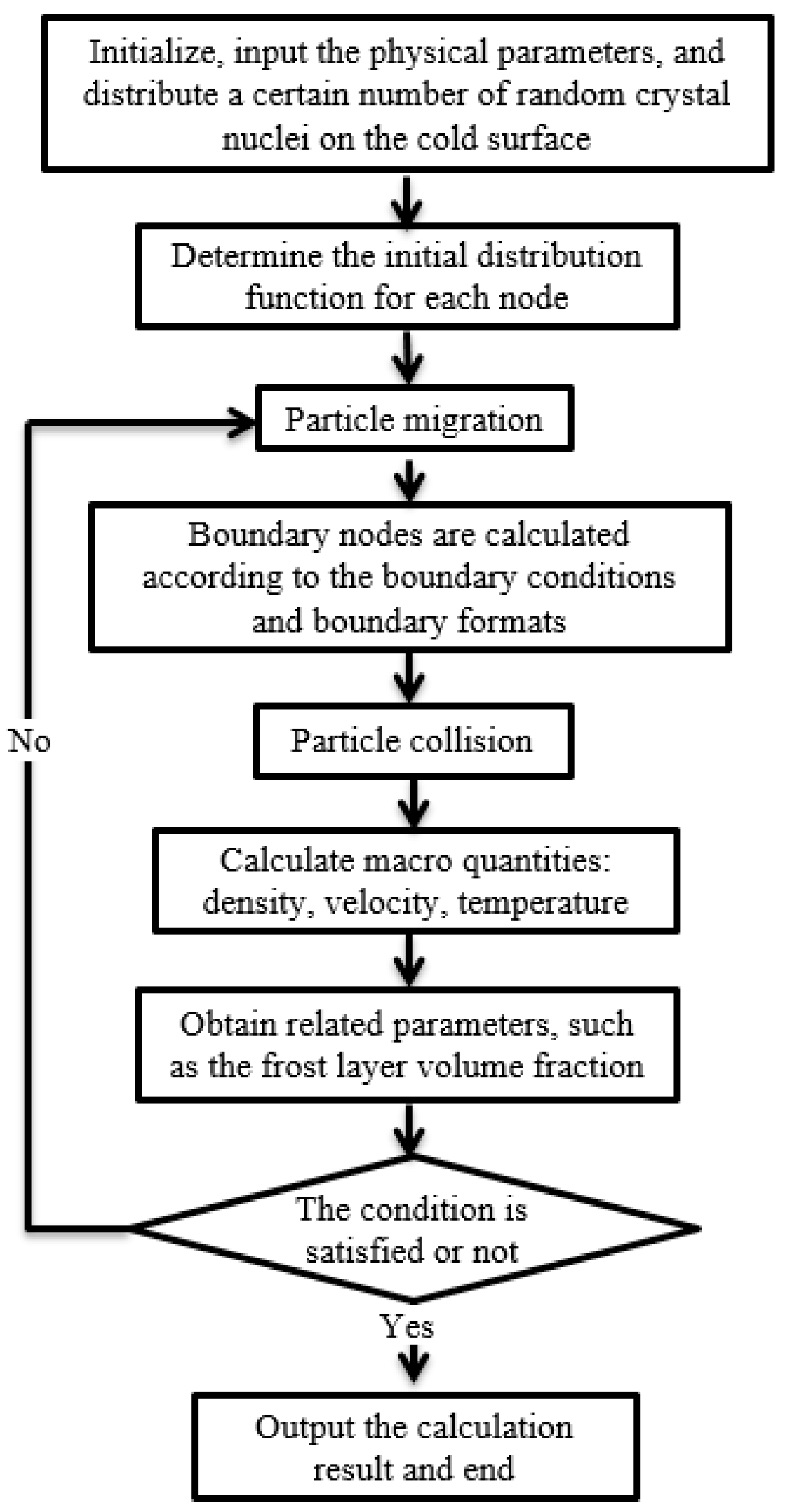
Figure 3.
Comparison between simulation results and experimental data [19].
Figure 3.
Comparison between simulation results and experimental data [19].
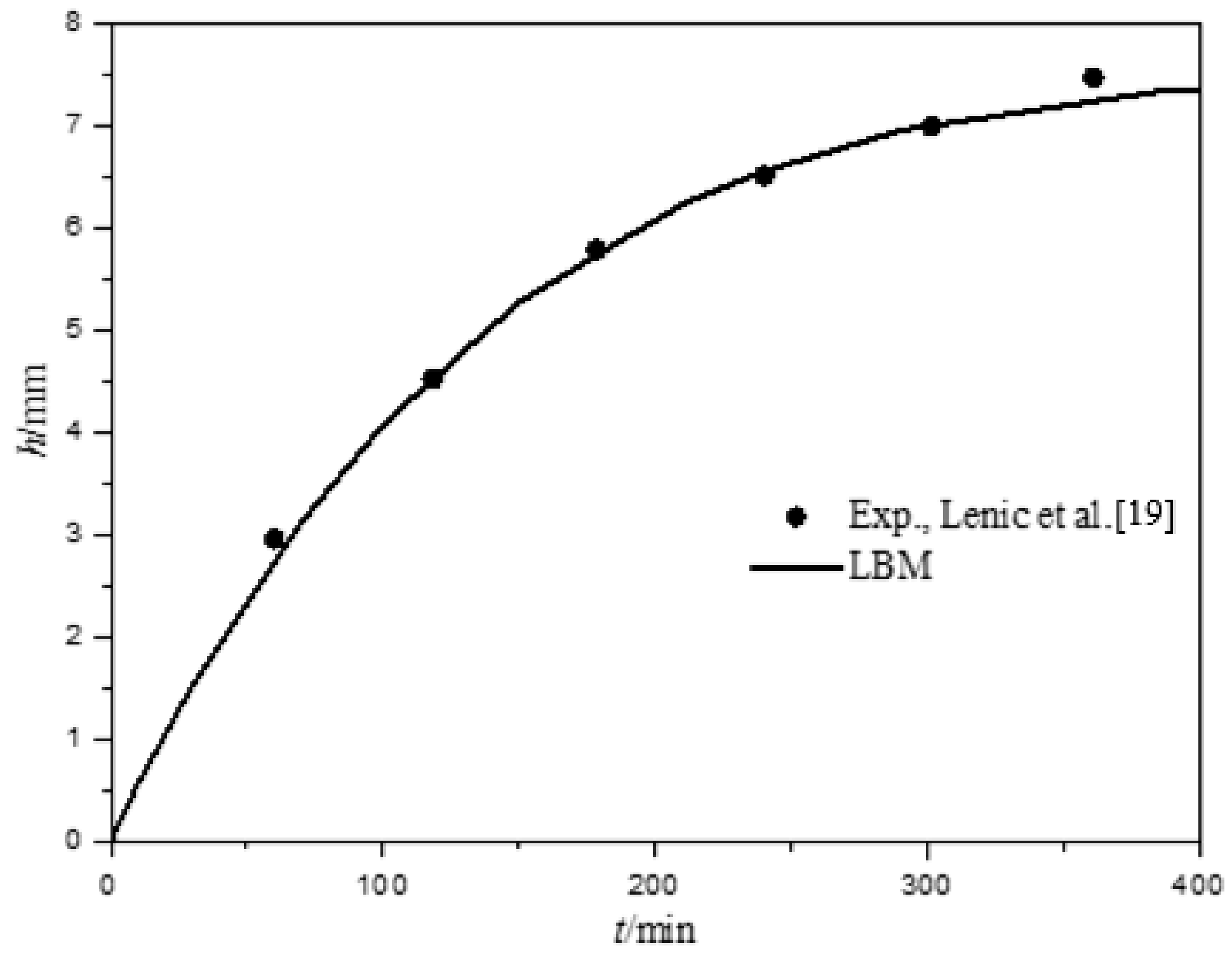
Figure 4.
Variation of average density of the frost layer over time.
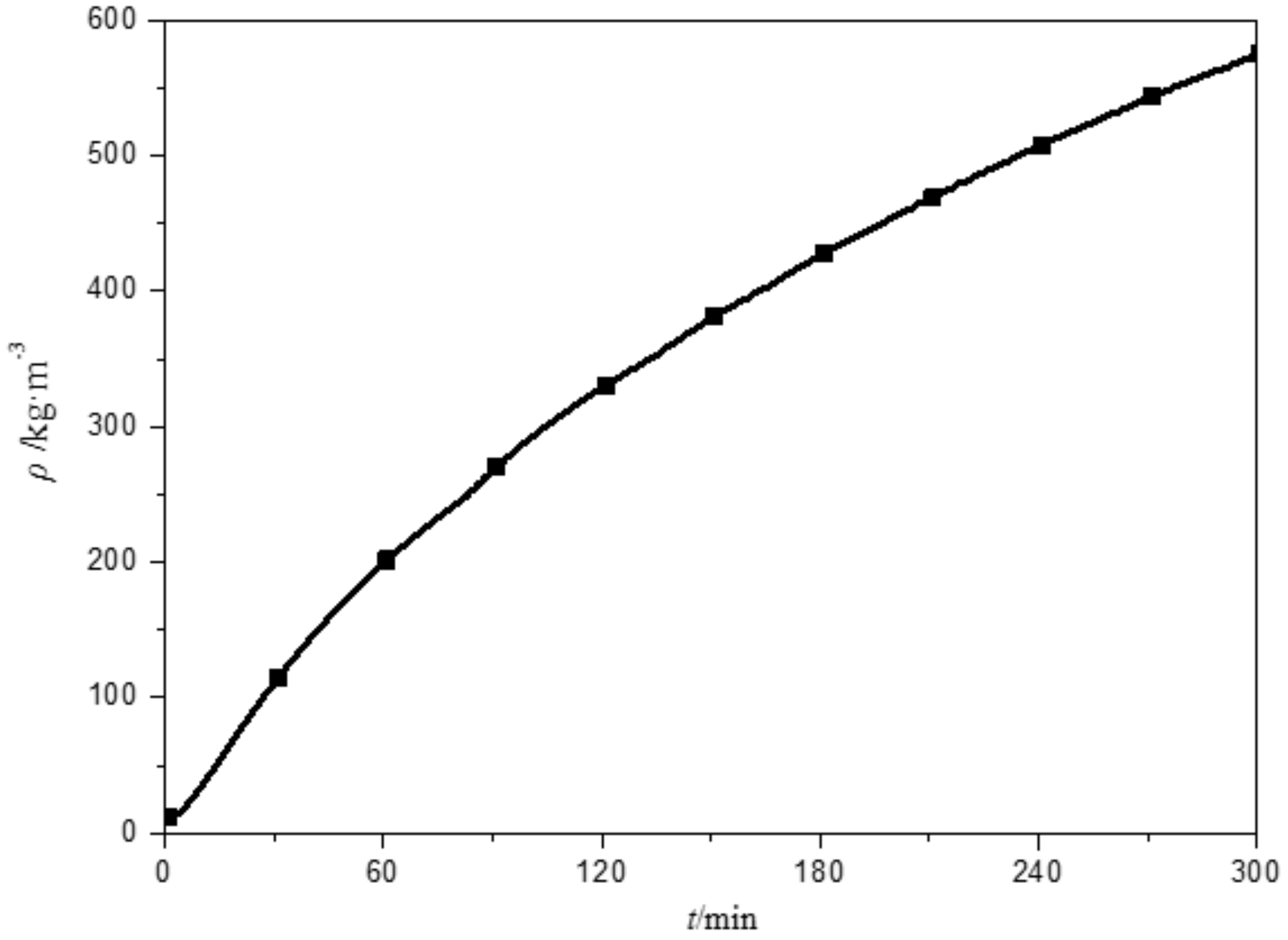
Figure 5.
Variation of frost thickness over time.
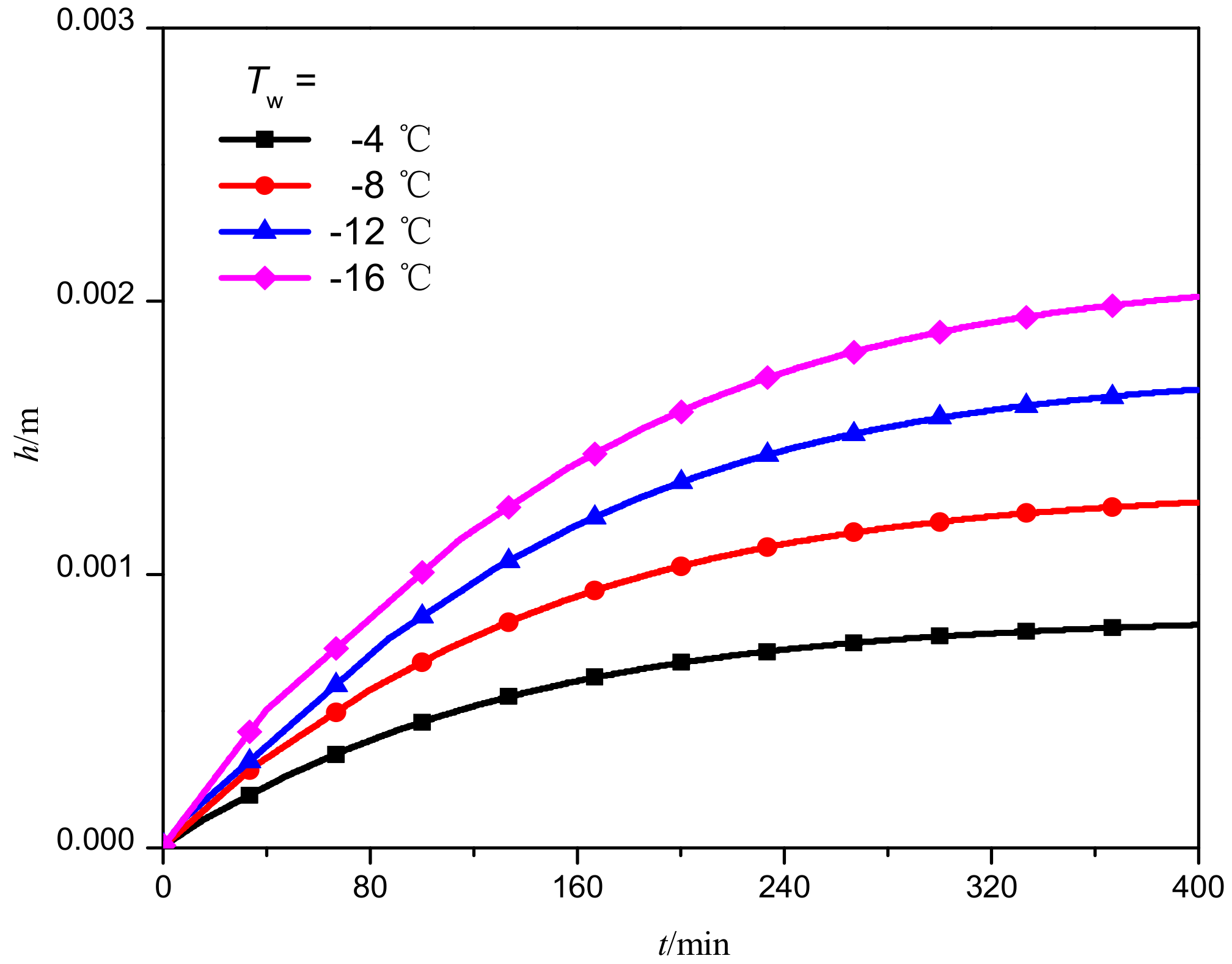
Figure 6.
Variation of frost deposition over time at different cold surface temperatures.
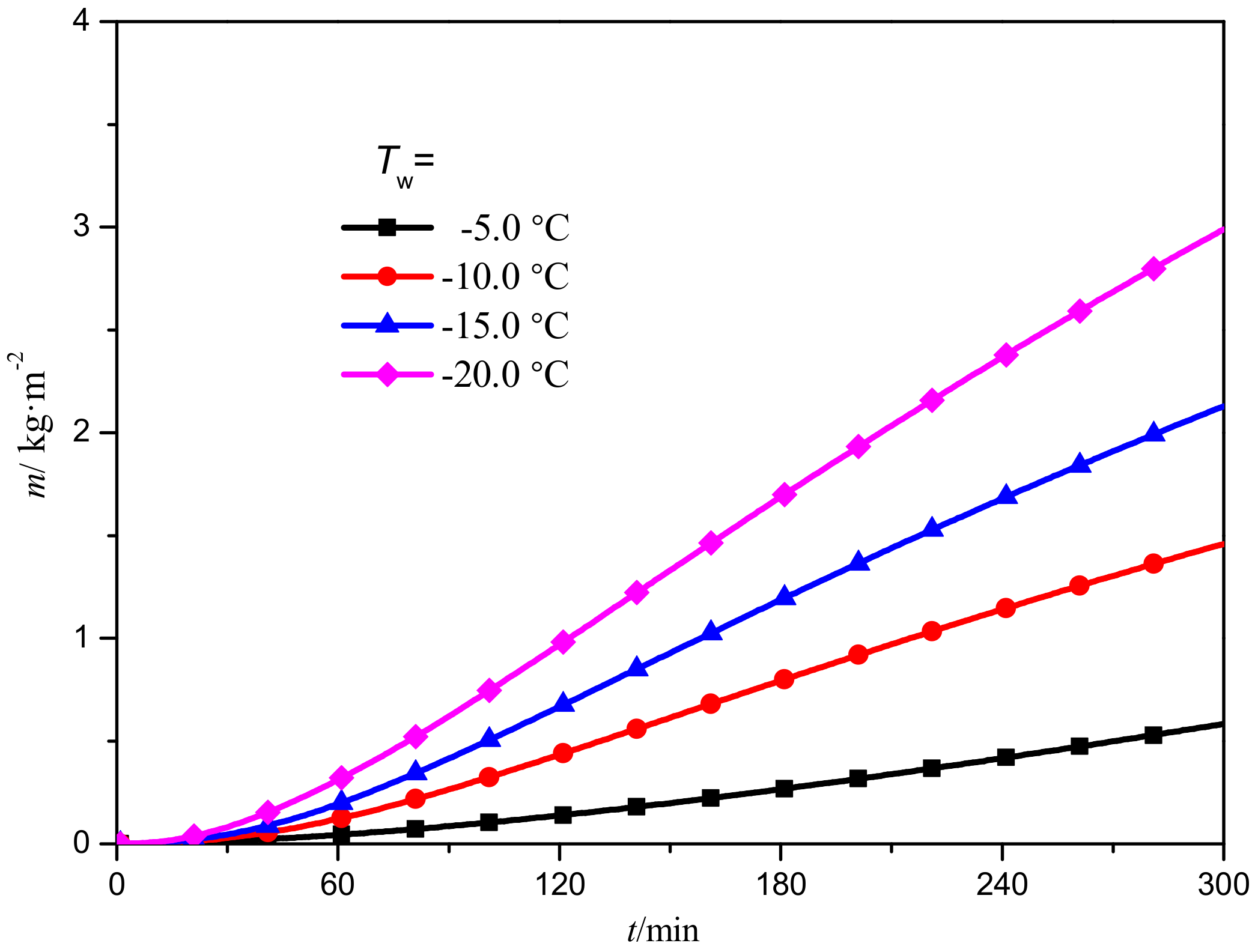
Figure 7.
Variation of frost crystal deposition rate over time at different cold surface temperatures.
Figure 7.
Variation of frost crystal deposition rate over time at different cold surface temperatures.

Figure 8.
Distribution of frost crystal volume fraction in the frost layer.

© 2018 by the authors. Licensee MDPI, Basel, Switzerland. This article is an open access article distributed under the terms and conditions of the Creative Commons Attribution (CC BY) license (http://creativecommons.org/licenses/by/4.0/).
Share and Cite
MDPI and ACS Style
Gong, J.; Hou, J.; Sun, J.; Li, G.; Gao, T. A Numerical Investigation of Frost Growth on Cold Surfaces Based on the Lattice Boltzmann Method. Energies 2018, 11, 2077. https://doi.org/10.3390/en11082077
AMA Style
Gong J, Hou J, Sun J, Li G, Gao T. A Numerical Investigation of Frost Growth on Cold Surfaces Based on the Lattice Boltzmann Method. Energies. 2018; 11(8):2077. https://doi.org/10.3390/en11082077
Chicago/Turabian StyleGong, Jianying, Jianqiang Hou, Jinjuan Sun, Guojun Li, and Tieyu Gao. 2018. "A Numerical Investigation of Frost Growth on Cold Surfaces Based on the Lattice Boltzmann Method" Energies 11, no. 8: 2077. https://doi.org/10.3390/en11082077
Note that from the first issue of 2016, this journal uses article numbers instead of page numbers. See further details here.