Article

A Fractional Order Power System Stabilizer Applied on a Small-Scale Generation System

by
Florindo A. de C. Ayres Junior
1,*,
Carlos T. da Costa Junior
2,
Renan L. P. de Medeiros
1,
Walter Barra Junior
2,
Cleonor C. das Neves
3,
Marcelo K. Lenzi
4 and
Gabriela De M. Veroneze
5
1
Department of Electricity, Faculty of Technology, Federal University of Amazonas, Manaus 69080-900, Brazil
2
Electrical Engineering Faculty, Institute of Technology, Federal University of Pará, Belém 66075-110, Brazil
3
Federal Institute of Amazonas, Manaus 69075-351, Brazil
4
Chemical Engineering Department, Federal University of Paraná, Curitiba 81531-980, Brazil
5
Department of Engineering of Production, Faculty of Technology, Federal University of Amazonas, Manaus 69080-900, Brazil
*
Author to whom correspondence should be addressed.
Energies 2018, 11(8), 2052; https://doi.org/10.3390/en11082052
Submission received: 3 July 2018 / Revised: 21 July 2018 / Accepted: 1 August 2018 / Published: 8 August 2018
(This article belongs to the Section F: Electrical Engineering)

Abstract

:
In this paper, a Fractional Order Power System controller (FOPSS) is designed, and its performance and robustness are experimentally evaluated by tests in a 10 kVA laboratory scale power system. The FOPSS design methodology is based on the tuning of an additional design variable, namely the fractional order of the controller transfer function. This design variable is tuned aiming to obtain a tradeoff between satisfactory damping of dominant oscillating mode and improved closed-loop system robustness. For controller synthesis, transfer function models were estimated from data collected at selected operating points and subsequently applied for the controller design and for obtaining upper bounds estimates on the operating-point depends on plant uncertainties. The experimental results show that the FOPPS was able to obtain a robust performance for the considered set of the power system operating conditions.

1. Introduction

Due to the continuously growing electrical energy demand, electric power systems need to be operated close to their stability limits [1]. Consequently, new research on advanced and intelligent control techniques is required to improve the system stability margins. In particular, the dominant electromechanical oscillation mode must be well-damped for the range of allowed operating conditions to preserve system stability and to assure safe operation. To accomplish this task, Power System Stabilizers (PSS) are used to improve the damp of dominant oscillation mode in the interconnected power system [2]. Research on new advanced control for PSS performance improvment is a very active field in control system engineering. Therefore, many studies, including on adaptive control [3], gain-scheduling fuzzy control [4] and robust control [5], to name a few, have been carried out in the last two decades. A promising robust control strategy whose potential is now being investigated in different engineering applications is Fractional Order Control. Fractional order controllers can be seen as a natural extension of conventional control techniques [6]. Considerable attention in fractional order controllers have been carried out in recent years, mainly because of their additional design parameters gives a more flexible degree of freedom on the design task when compared to conventional Lead-Lag controllers [6]. Some applications of fractional control are discussed in [7], where a Fractional Order PID (FOPID) is investigated to track a servomechanism position with actuator nonlinearity’s consideration. In [8], a FOPID tuning study is based on a Taylor’s series expansions method to design a regulating control for DC motors. The tuning of a fractional order Automatic Voltage Regulator (AVR) controller using the particle swarm optimization method is present in [9]. In [6], an auto-tuning method for fractional order controllers is presented along with practical tests carried out in a Basic Process Rig 38–100 Feedback Unit industrial device to control the water column level. Indeed, three of the works mentioned above only present simulation results, which demonstrates a need for experimental works to validate fractional order based control strategies in real engineering systems.
In this paper, the application of fractional order control in a real-world laboratory power system is reported to assess the potential of this control methodology in real power systems. A fractional order damping controller is designed, and its performance is evaluated by performing a set of experimental tests in a 10 kVA power system for a range of allowed operating conditions. The authors believe that the main contribution of this paper is on providing a link between real-world practical power system applications and fractional control theory. The proposed fractional order based approach is implemented as a fixed-parameter digital control law which presents some robustness properties to cope with variations on the plant operating conditions. No adaptive approaches were investigated. The main contribution of this paper can be summarized as follow:
Novel methodology to design PSS based on fractional-order network compensator, emphasizing the novel form to choose α parameter.
Experimental assessment of PSS based on fractional-order applied on generates a system in small scale.
The remainder of this paper is organized as follows: Section 2 presents a brief introduction to fractional order systems. Section 3 presents the tuning method for the classical power system stabilizer and the fractional order power system stabilizer. In Section 4, after a brief description of the 10 kVA laboratory power system, the identification tests for local model identification is presented and discussed. Section 5 presents the design of both fractional PSS (FOPSS) and conventional PSS. In Section 6, a robustness assessment of the designed controllers regarding a set of operating pointing dependent plant uncertainties is performed. Section 7 presents and discusses the results of experimental tests performed in a small-scale power plant. Finally, in Section 8, the conclusions of this study are presented.

2. Fractional Order System

2.1. Background of Fractional Order System in the Frequency Domain

A fractional order operator may be described as
D a t q = { 1 Γ ( t τ ) 0 t f ( m ) ( τ ) ( t τ ) ( q + 1 m ) d τ ,   for   m 1 < q < m d m d t m f ( t ) ,   for   q = m    
Γ ( t z ) = 0 t z 1 e t d t ,
where q is a rational number, defining the fractional order, and a and t are the limits for the derivative and the integral operators. This fractional order operator definition is known as Caputo’s definition [10,11].
Because the Laplace transform is widely used for control analysis and design, it is usually useful expressing the fractional order operator in its frequency domain version, by using the Laplace´s transform of Equation (2), as follows
L { D 0 t α f ( t ) } = s α F ( s ) , α   ,
where null initial conditions have been assumed in Equation (3).

2.2. Phase and Gain Contributions Due to Fractional Order Lead-Lag System

A fractional order system is defined in the following form,
F ( s ) = ( s T 1 + 1 ) α ,
By using s = jω, the corresponding magnitude and phase are given by:
20 log 10 | ( j ω T 1 + 1 ) α | = 20 log 10 | ( j ω T 1 + 1 ) | α = 20 α log 10 1 2 + ( ω T 1 ) 2 ,
( j ω T 1 + 1 ) α = α a r c t g ( ω T 1 ) ,
It can be seen, from Equations (5) and (6), that both magnitude and phase contributions can be controlled by setting the value of the fractional order parameter α. Therefore, besides the time constant T1, the fractional order parameter α allows for an additional degree of freedom for the design of damping controllers. This property will be exploited in the next sections to design fractional order based PSS.

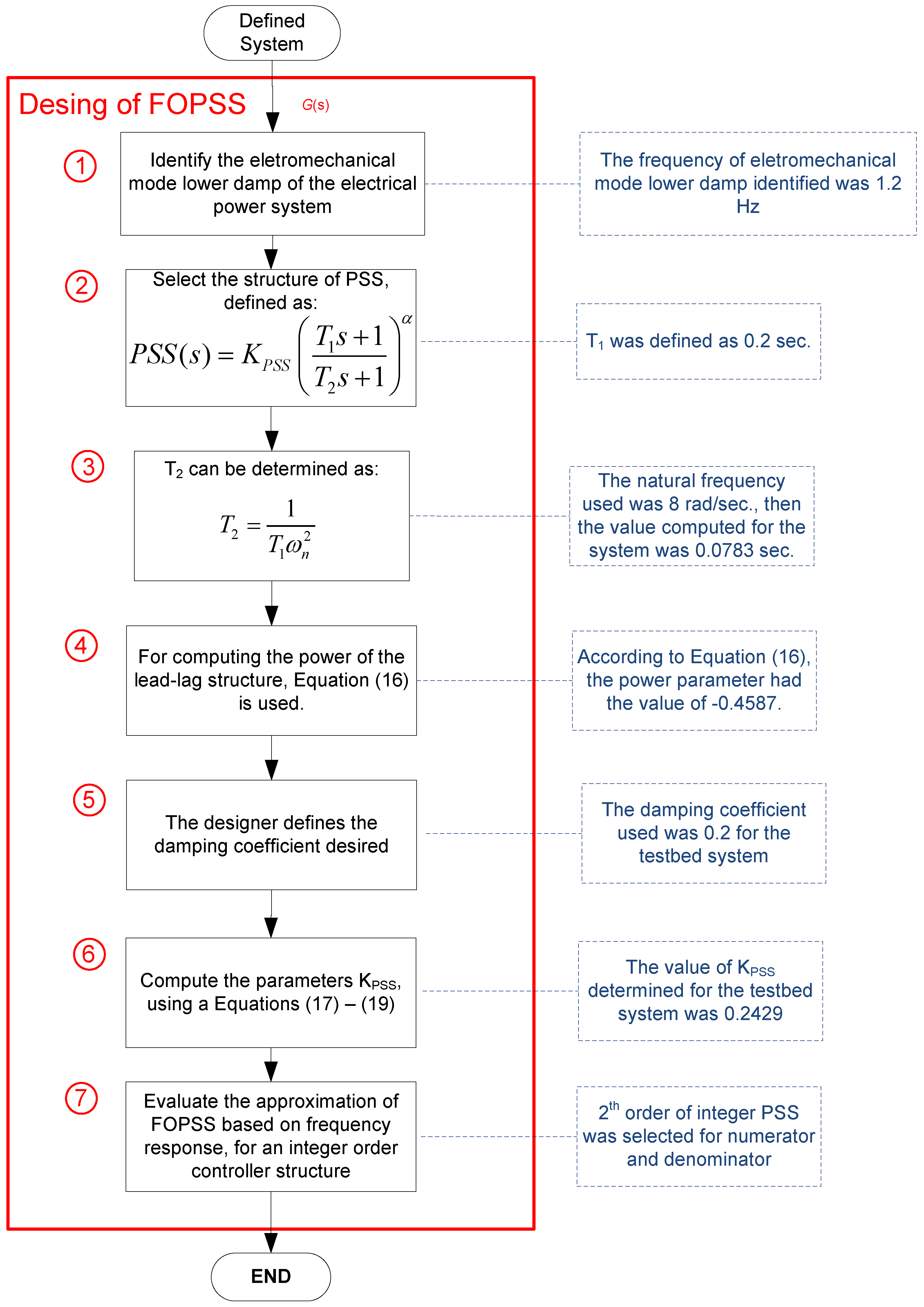
3. Tuning Method for Fractional Order Power System Stabilizer

3.1. Classical Tuning Method for Power System Stabilizer

To tune the conventional PSS compensator as well as the fractional compensator, GEP(s) represents the dynamics from Automatic Voltage Regulator (AVR) set point increment to the corresponding increment on the electrical torque component via excitation system. In this work, this transfer function was obtained by using the experimental identification method previously presented in Section 4. The classical Lead-Lag compensator tuning method was obtained based on the methodology proposed in the seminal paper by Larsen and Swann [12]. This standard method is based on phase compensation design followed by PSS gain tuning by using the root-locus method. The Lead-Lag Classical transfer function is given by Equations (7) and (8):
P S S ( s ) = K P S S P S S ' ( s ) ,
P S S ' ( s ) = ( T 1 s + 1 T 2 s + 1 ) 2 .
Step 1: Use the obtained electromechanical natural frequency value shown previously in Figure 1; find the phase needed to accomplish phase compensation of Lead-Lag Compensator; and choose the value of the parameter T1. Typical values of the parameter T1 are within 0.2–1.5 s [2], applying Equations (9) and (10):
P S S ' ( s ) | j ω n + G E P ( s ) | j ω n + G ( s ) | j ω n = 0 ,
T 2 = 1 ω n ( arctan ( ω n T 1 ) arctan ( P S S ( j ω n ) ) 2 ) .
Step 2: Find the desired Torque damping coefficient to tune KPSS gain, applying Equation (11):
D P S S = 4 H ω n ξ d ω o .
Step 3: Find the Lead-Lag compensator gain, applying Equations (12) and (13):
D P S S = K P S S | G E P ( j ω n ) | | G ( j ω n ) | | P S S ' ( j ω n ) | ,
K P S S = D P S S | G E P ( j ω n ) | | G ( j ω n ) | | P S S ' ( j ω n ) | .

3.2. Fractional Order Compensator Tuning Method

The tuning of the FOPSS parameters is accomplished by using a frequency domain approach which consists in extending the classical PSS design to calculate the parameters of the compensator, raised to a fractional power value. The fractional power parameter enables shaping the desired closed-loop frequency. Therefore, to design FOPSS, this section presentes a sequence of four steps: Steps 1–3 are to find parameters of Lead-Lag compensator, while, in Step 4, the gain tuning is performed:
Step 1: Find natural electromechanical frequency modes with a low damping ωn.
Step 2: Choose T1 parameter value, and then find T2 parameter value by using Equation (14):
T 2 = 1 T 1 ω n 2 .
Remark 1: In Step 2, the phase condition imposes a single equation having two unknown variables, namely the values of time constants T1 and T2. As a possible choice, the value of T1 has been fixed at the same value obtained for the conventional PSS and T2 has been calculated using Equation (14).
Step 3: Applying Equations (15) and (16), the fractional order power α is found:
α ( arctan ( ω n T 1 ) arctan ( ω n T 2 ) ) = arctan ( F O P S S ' ( j ω n ) ) ,
α = F O P S S ' ( j ω n ) ( arctan ( ω n T 1 ) arctan ( ω n T 2 ) ) .
Step 4: After parameters T1, T2 and α have been calculated, the value of KPSS gain is then obtained by specifying a desired damping coefficient ξd and using the modulus condition, as follows:
D F O P S S = 4 H ω n ξ d ω o ,
D F O P S S = K F O P S S | G E P ( j ω n ) | | F O P S S ' ( j ω n ) | ,
K F O P S S = D F O P S S | G E P ( j ω n ) | | F O P S S ' ( j ω n ) | .
Finally, the transfer function of Fractional Order PSS (FOPPS) is obtained in the following fractional order Lead-Lag [13,14] form:
F O P S S ( s ) = K F O P S S ( T 1 s + 1 T 2 s + 1 ) α .

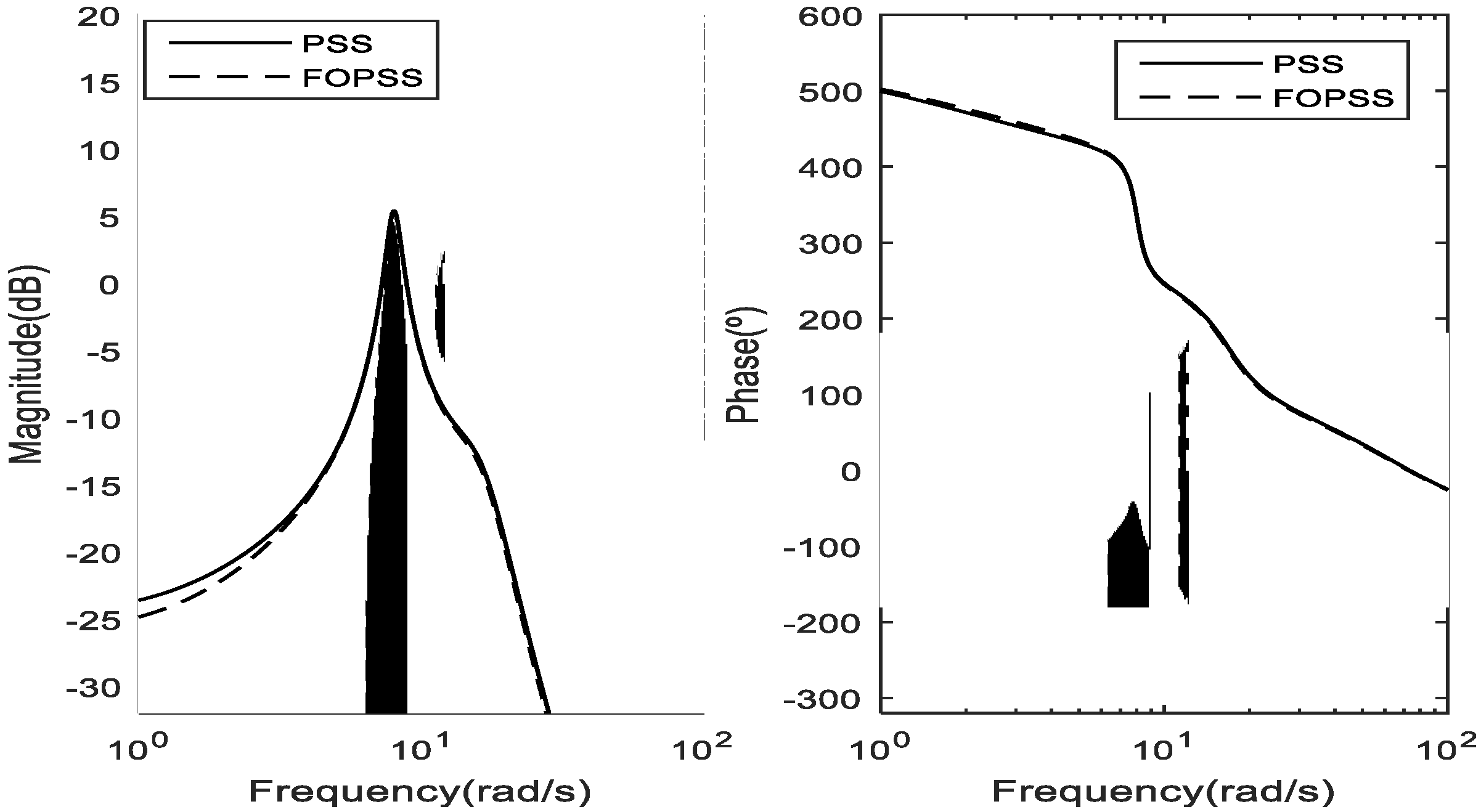
3.3. Fractional Order Approximation

After its design, real-world implementation of the fractional order controller must be done. This task is carried out by searching for an integer order dynamic system which approximates the dynamic behavior of the designed fractional order controller in a specified frequency range. In this work, the approach proposed in [14], which is based on pole-zero network synthesis is adopted. This approach can be outlined by the following steps [14]:
Step 1: Get the exact frequency response of fractional order system.
Step 2: Select an appropriate order for the numerator and denominator of the approximating integer order system, in a range of frequencies of interest (for PSS design, this range can be, for instance, the range of frequencies containing the frequencies of the target electromechanical oscillating modes).
Step 3: Find the values of the parameters (values of poles and zeros) of the approximating integer order model by using the invfreqs function, in the Matlab R2015a software.
Step 4: Verify if the obtained controller satisfies the desired performance behavior. If the control objective was not reached, then return to Step 2 and select other values for the numerator and denominator order or modify the range of frequencies of interest.

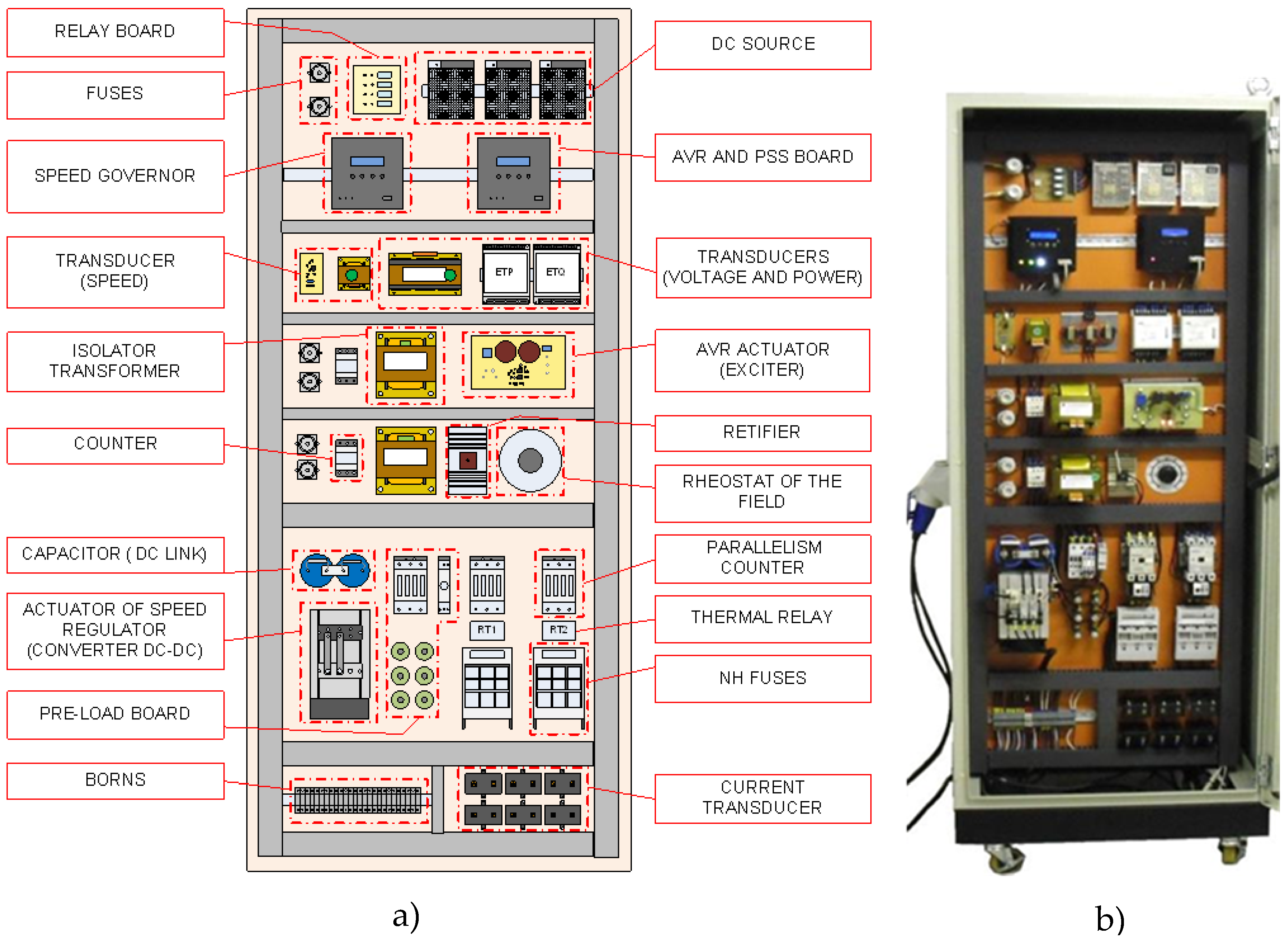
4. Laboratory Power System and Identification Tests

4.1. Small-Scale 10 kVA Power System

Controller evaluation was performed in a small-scale power system comprised of a synchronous generating unit (10 kVA, 220 VRMS, 60 Hz), a transmission line model, transformers, as well as measurement and control subsystems (Figure 2a). The system has a typical machine-infinite bus bar power system configuration (Figure 2b). The synchronous generator was specially built so that its physical parameter values are similar, in per unit values, to that of large synchronous generators. An inductive branch represents a typical short transmission line. Table 1 presents the corresponding values for some nominal values of physical parameters of the laboratory power system. The synchronous generator unit is equipped with a fast-actuating field excitation system based on a DC-DC buck converter. The automatic voltage regulator (AVR) is of proportional type, as described in [4], by the same research group of this paper.

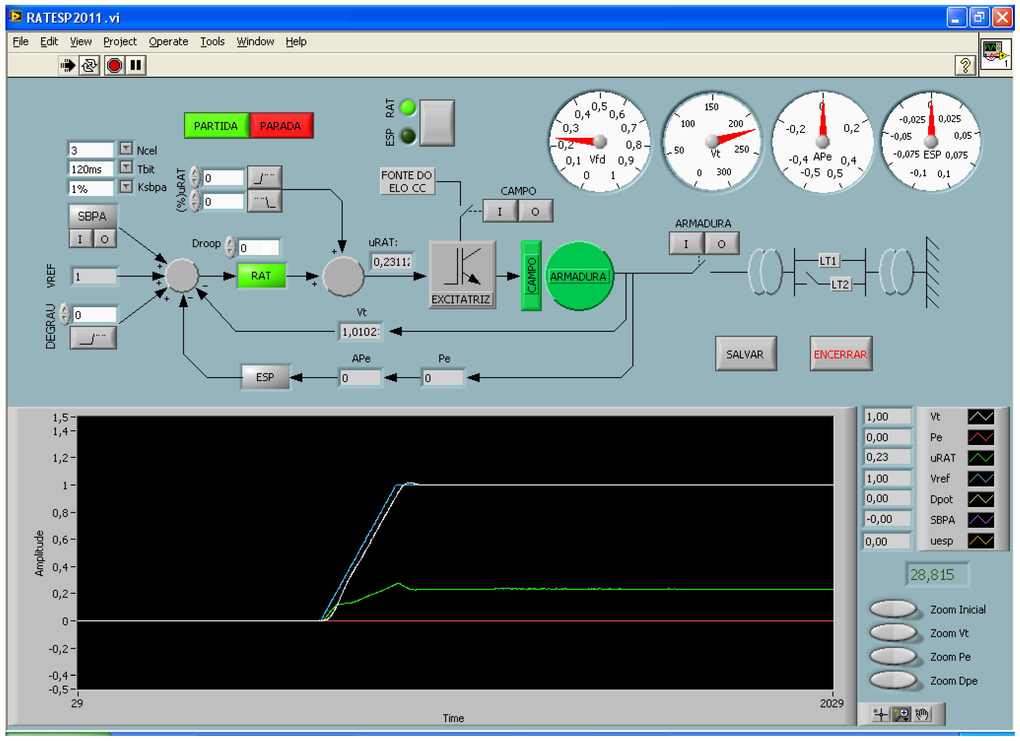
4.2. Experimental Environment

The control and drive panel is installed in an industrial standard panel where the components responsible for the activation and small-scale 10 kVA power generation system control are installed. This panel comprises the components responsible for the drive, measurement of current and voltage signals necessary for the system operation. Figure 1 presents a control panel design scheme and a panel photograph are shown. The Exciter actuator is a DC-DC buck power converter that controls the synchronous machine rotor current directly, the microcontroller that the embedded systems control laws of AVR and PSS is a Microchip dsPIC 30F4011.
In Figure 3, the AVR and PSS graphical man–machine interface (MMI) is shown. The MMI that operates the digital AVR and PSS has a set of keys to send commands directly to the instrument and numerical and graphical displays to show several parameters and signals during operation.

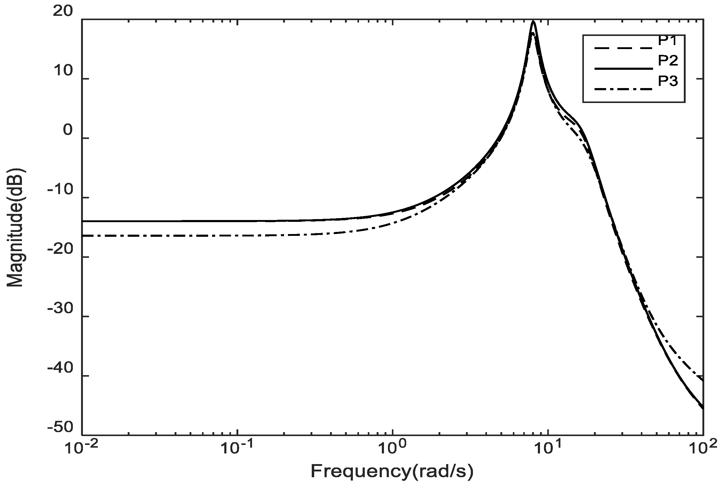
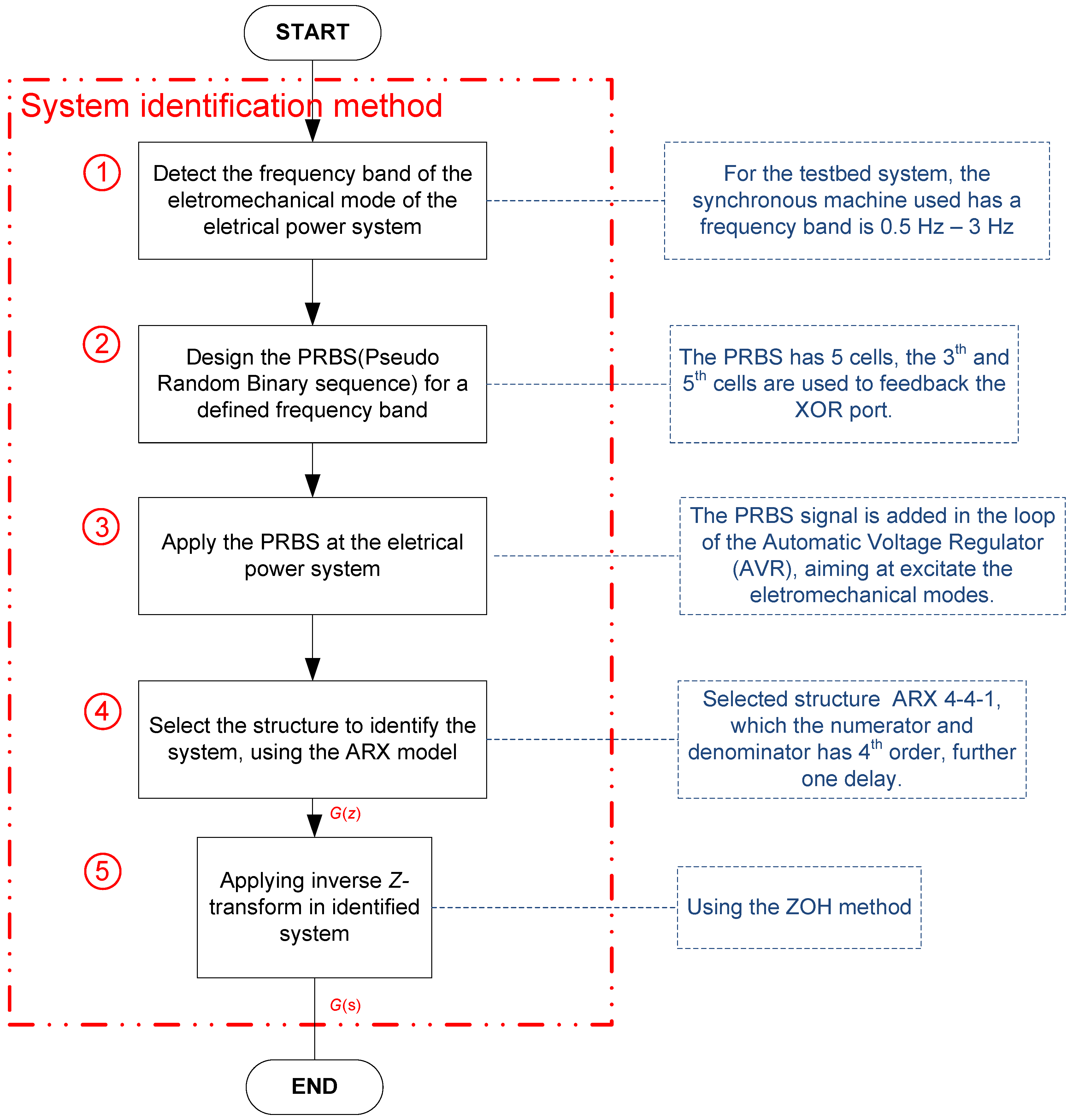
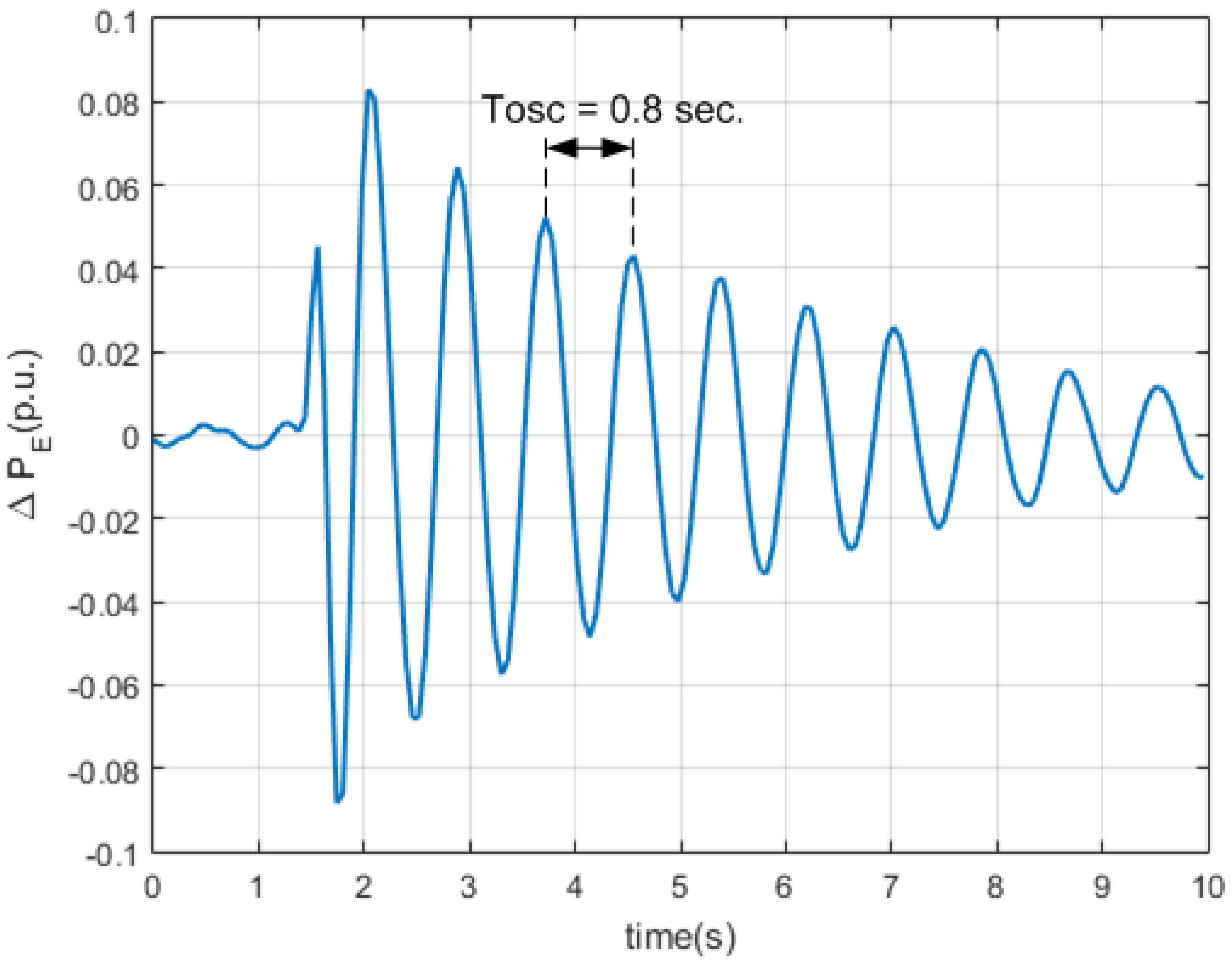
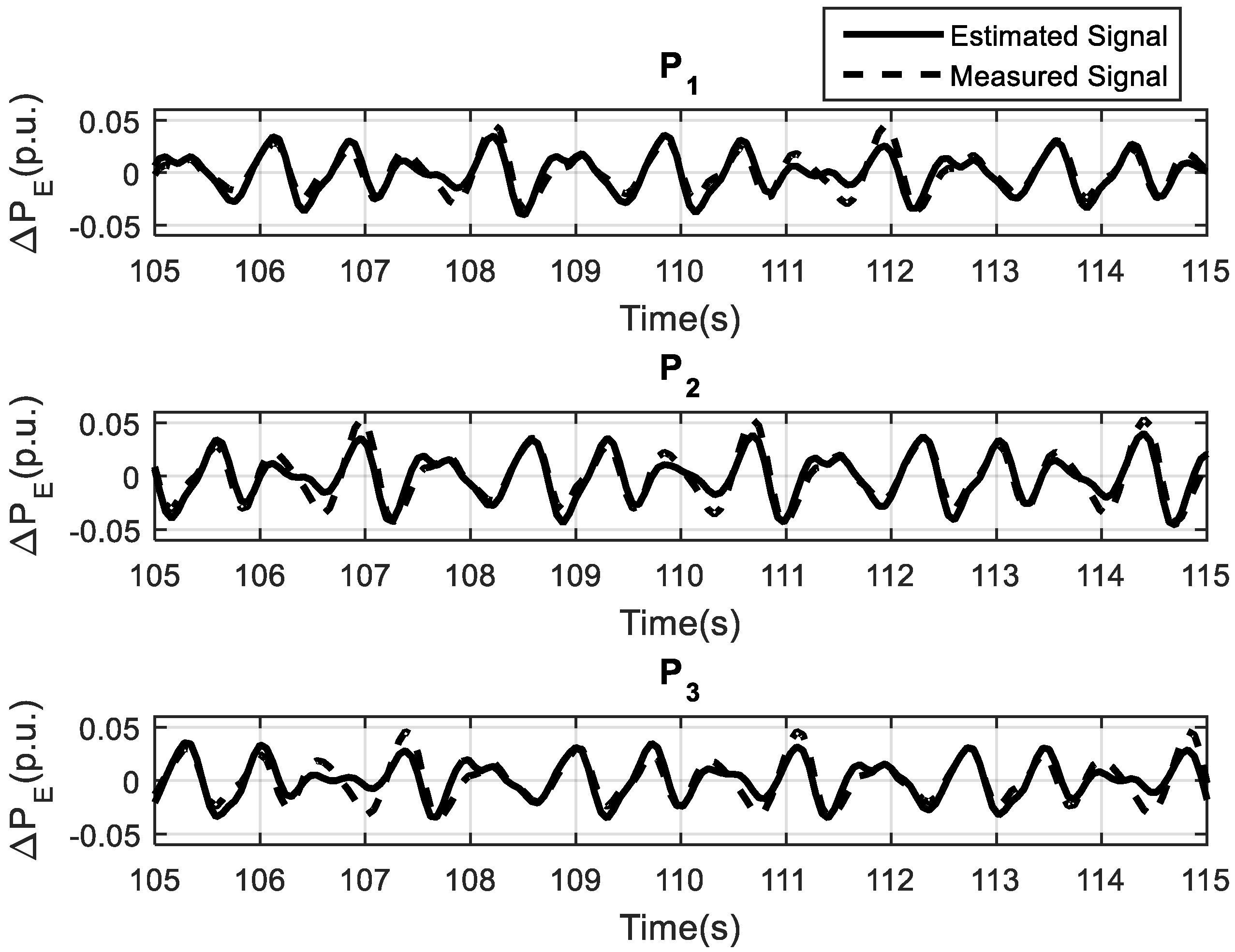
4.3. System Identification Tests

The power system presents a nonlinear dynamic behavior which depends on its operating condition. To represent the relevant dynamic around a set of representative operating state, a set of discrete-time linear Autoregressive with Exogenous Input (ARX) are constructed, having a structure giving by Equation (21),
B ( q 1 ) A ( q 1 ) = q d ( b 1 + b 2 q 1 + ... + b n B q n B ) 1 + a 1 q 1 + ... + a n A q n A .
where q−1 is the unitary delay operator and A(q−1), and B(q−1) are, respectively, the denominator and the numerator polynomials whose value of the parameters vector θ ^ = [ b 1 , b 2 , ... , b n B , a 1 , a 2 , ... , a n A ] T is estimated by using a standard Least Mean Square parameter estimation approach [15]. The obtained ARX models are then subsequently applied for both controller design and robustness analysis tests.
Operating points corresponding to three different level of the generator loading levels “LOW”, “MEDIUM” and “HIGH”, corresponding, respectively, to generated active power Pe = {0.3, 0.5, 0.65} p.u. For all the selected operating conditions, the magnitude of the generator terminal voltage was kept close to its nominal value (VT equal to 1.00 p.u.), while the value of generated reactive power was kept close to 0 p.u. Figure 4 shows the results of the measured active power response for small pulse disturbance applied in superposition to the AVR setpoint value. The operating point of this test corresponds to the MEDIUM loading condition (Pe = 0.5 p.u.). A dominant oscillation mode, having a natural period around TOSC = 0.8 s, can be observed. This dominant oscillation mode presents very low damping and, therefore, a Power System Stabilizer (PSS) must be designed to provide sufficient damping for this dominant mode. By using the estimated value of TOSC, a suitable value for the sample time value must satisfy TS << TOSC and, therefore, a sample time value of TS = 0.060 seconds has been chosen for both data acquisition and control objectives.
A Pseudo Random Binary Signal (PRBS) was designed to excite uniformly the system modes in the range of frequencies from 0.5 to 3 Hz, which includes the nominal range for the local mode in power studies. Small amplitude (0.01 p.u.) for the PRBS signal was selected in order not to disturb the terminal voltage regulation considerably. A set of equations to implement the PRBS signal as in [15], is given by Equations (22)–(27):
1 10 f m a x T b i t 1 10 f m a x  
T b i t = 1 3 f max = 1 9 120 m s  
f min = 1 ( 2 N 1 ) T b i t  
2 N 1 = 1 f min T b i t = 1 0 , 06  
2 N 1 = 17 2 N = 18  
N = 5  
The estimated spectrum obtained by processing the collected data is shown in Figure 5, where can be observed that the system has a dominant oscillating mode whose natural frequency is close to 1.2 Hz, which is poorly damped without using a PSS damping controller.
Using the recorded input–output data, considering the PRBS signal as the system input and measured active power deviation as the system output, fourth order ARX models, having the structure given in Equation (21), were estimated for the power system operating around LOW, MEDIUM and HIGH loading conditions, corresponding, respectively, to following levels of generated electric active power: Pe = {0.30, 0.50, 0.65} p.u. These identified local models are named P1, P2, and P3, respectively. The corresponding values for parameters of the local models P1, P2 and P3, were obtained using standard Least Mean Square (LMS) estimation techniques [15] and are provided in Table 2.
In Figure 6, it can be observed that a satisfactory fitting has been obtained between the output estimated by using the local models P1, P2, and P3 and the real output measurements. This confirms that the identified models are accurate enough for control design purposes as these models were able to capture the frequency of the target oscillation mode and, therefore, the model is suitable for PSS control design. Additional standard validation tests based on correlation analysis, not shown, confirmed the adequacy of the identified model.
In Figure 7, the magnitude frequency response obtained from the estimated local models P1, P2, and P3 is shown. It can be observed that, for all three models, the value of natural frequency of the dominant mode is around 8 rad/s. Furthermore, the damping for this target mode changes substantially with the operating condition. Such variability makes the design of robust PSS controller a quite challenging task.
The corresponding eigenvalues computed for the local models P1, P2 and P3 are provided in Table 3, where ξi(j) and ωi(j) are the respective values of relative damping and the natural frequencies of the i-th eigenvalue, λi, i = 1, 2, 3, 4, calculated for each identified local models Pj, j = 1, 2, 3. It can be observed that the relative damping of dominant the eigenvalue is very low, indicating that the power system presents reduced stability margins.
A flowchart that describes all five steps applied to identify the plant models is presented in Figure 8. In Step 1, the frequency band where lies the natural electromechanical modes is selected. In Step 2, the PRBS signal is designed. In Step 3, the PRBS signal in the AVR control loop is applied to excite the system. In Step 4, the ARX model structure is selected. In Step 5, the continuous model is obtained, by applying the inverse z transform ZOH method, using sampling time equal to 0.06 s.

5. Design of the Fractional Order PSS and Tests in the 10 kVA Laboratory Power System

For design purposes, in the following, the nominal model P0 has been taken to be P0 = P2, namely the local model identified for the MEDIUM loading operating condition of the power system (see Table 2). The rationale for this choice is that the MEDIUM loading shows to be the most frequent operating condition for the studied laboratory power system. The design objective is to increase the damping of the observed dominant oscillation mode, without changing substantially its natural frequency. Hence, a desired damping ξd = 0.2 has been specified for the dominant oscillating mode. A Fractional Order PSS (FOPSS) (having the structure given by Equation (28)), has been designed. The parameters of the FOPSS controller, namely KFOPSS, T1, T2 and α (the fractional order), were computed by using the algorithm steps already presented in Section 3 of this paper and their obtained values are provided in Table 4.
F O P S S ( s ) = K F O P S S ( T 1 s + 1 T 2 s + 1 ) α .
For performance comparison purposes, a conventional PSS (having two similar first-order Lead-Lag blocks) has also been designed by using the same nominal design specifications as stated above for the fractional order PSS design. This conventional PSS has been designed by using a standard classical technique [12,16]. Such classical design consists of performing a phase compensation step (allowing to obtain the values for the parameters N (number of Lead-Lag blocks) and time constants T1 and T2), followed by an adjustment of the PSS gain value, KPSS, by using the root-locus technique. This KPSS last tuning step has been performed by taking care for not to reduce the damping of the remaining system’s modes substantially. The values of the parameters for the conventional PSS are also provided in Table 4. To summarize, the proposed methodology is presented as a simplified flowchart in Figure 9.
A flowchart where all steps applied to identify the plant models is presented in Figure 7. In a the sequence of choosing the model to tune the controller, the following technique is applied. Firstly, in Step 1, the electromechanical low damping mode related to the desired frequency low damping ωn is identified. In Step 2, the T1 time constant values linked to the zero of the FOPSS is chosen as 0.2 s. In Step 3, the value of T2 time constant associated with the FOPSS denominator is computed and its value is 0.0783 s. In Step 4, the relation for computing the fractional parameter, α, carried out by Equation (16) is presented. In sequence, Steps 5 and 6 are related to obtaining the KFOPSS value of 0.2429. Finally, to allow for real-world FOPPSS implementation, its infinite dimensional transfer function (Equation (28)) must be approximated by using a finite dimensional (integer order) transfer function. This finite order approximation is held in the frequency band ω ∈ [0.01, 100] rad/s and is selected second to implement the structure of compensator. This order is chosen due to the great fit obtained in the frequency band comparing structures of higher order given by Step 7.
To accomplish this task, a frequency domain interpolation method, proposed in Reference [14], has been applied to obtain the corresponding finite order FOPSS controller approximation given by Equation (29):
C F O P S S ( s ) = 0.158 s 2 + 3.017 s + 13.59 s 2 + 15.54 s + 55.95 .
In Table 5, the eigenvalues computed for the nominal closed-loop nominal system are provided for both: the Conventional PSS and the FOPSS controllers. It can be observed that, in the nominal operating condition of the design, both controllers were able to satisfactorily improve the relative damping of the dominant oscillating mode as expected.
For the digital implementation of the FOPSS control law by using a DSPIC microcontroller chip, the FOPSS approximated transfer function, CFOPSS, given by Equation (21), has been discretized by using the Tustin method, with TS = 0.06 seconds sample time interval. Such discretization allows for representing the FOPSS control law by using a canonical RST standard structure given by Equation (30).
C ( q 1 ) = r 0 + r 1 q 1 + ... + r m q m 1 + s 1 q 1 + ... + s m q m .
Table 6 provides the corresponding values obtained for the coefficients of the digital law in Equation (22), for the designed FOPSS controller. Similar discretization steps were also performed for the designed conventional PSS, and the corresponding coefficients of the digital control law (in the form of Equation (30)) are provided in Table 6.

6. Robust Performance Assessments for the Designed Fractional Order Power System Stabilizer

To assess the robust performance of the designed Fractional Order Power System Stabilizer (FOPSS), a recently developed robust performance evaluation methodology [17] was applied. Such methodology is based on Robust Bode plots, which makes it both easy to understand and easy to apply. For the allowed frequency of interest, robust performance boundaries are established for allowed and forbidden regions in the magnitude and phase Bode Plots for the loop nominal loop transfer function L0FOPSS(s) = CFOPSS(s)P0(s), where CFOPSS(s) and P0(s) are, respectively, the designed FOPSS (its finite-dimensional approximation, given by Equation (29)) and the nominal plant model used in the controller design.

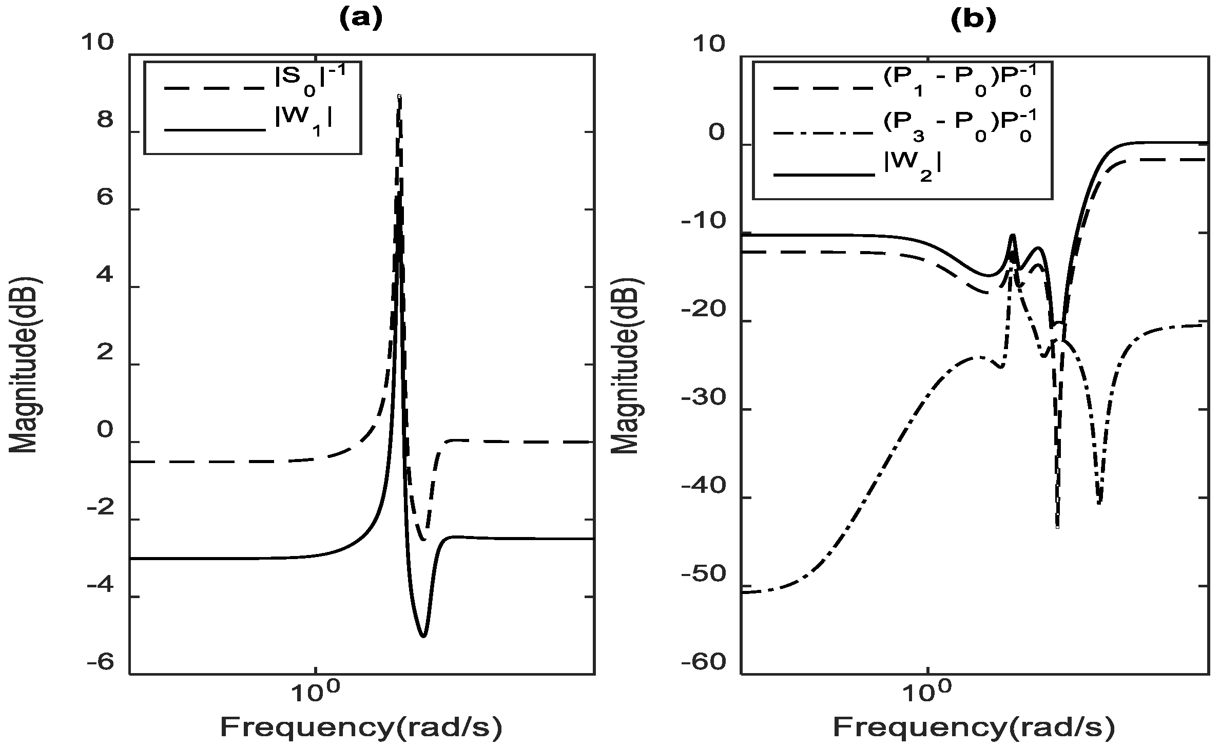
6.1. Robust Performance Boundaries Computation

In [18], it has been proven that a necessary and sufficient condition assuring the robust performance of a closed loop system composed by an uncertain plant model P(s) = P0(s) (1 + W2(s)Δ(s)) in unit negative feedback with a designed controller C(s) is given by,
| W 1 ( j ω ) | | S o ( j ω ) | + | W 2 ( j ω ) | | T o ( j ω ) | < 1 ,     ω   [ 0 , ] .
where P0(s) is the nominal plant model, Δ(s) is a multiplicative uncertainty satisfying Δ ( s ) < 1 , W1(s) and W2(s) are fixed stable weighting transfer functions, and S o ( s ) = 1 / ( 1 + C ( s ) P o ( s ) ) and T o ( s ) = 1 S o ( s ) are, respectively, the nominal sensitivity and complementary closed-loop transfer functions. W1(s) is a designer specified weighting stable transfer function satisfying W 1 ( s ) S o ( s ) < 1 .
By using the inequality in Equation (31) and by defining the nominal loop transfer function as being L o ( s ) = C ( s ) P o ( s ) , the following pair of coupled inequalities can be derived [17], considering ω [ 0 ] .
( 1 | W 2 | 2 ) | L o | 2 + 2 ( cos ( arg ( L o ) ) | W 1 | | W 2 | ) | L o | + ( 1 | W 1 | 2 ) > 0 ,
cos ( arg ( L o ) ) > ( | W 1 | 2 1 ) + 2 ( | W 1 | | W 2 | ) | L o | + ( | W 2 | 2 1 ) | L o | 2 2 | L o | ,
where the dependency on ω has been omitted for the sake of simplicity.
By specifying a range of frequencies of interest, the inequalities in Equations (32) and (33) are used to numerically computing bounds on the allowed and forbidden regions for | L o ( j ω ) | and arg ( L o ( j ω ) ) . These calculated bounds are then superimposed into the Bode plot (magnitude and phase) of L o ( j ω ) , for analysis purposes. Any observed intersection of | L o ( j ω ) | plot (or arg ( L o ( j ω ) ) ) with the computed robustness boundary regions given by Equations (32) and (33) mean that the designed controller fails to satisfy the robust performance for the considered set of uncertainties.
Therefore, the above described robust analysis methodology was applied to evaluate the robust performance of the designed FOPSS against the uncertainties due to the plant operational conditions.

6.1.1. Selecting the Nominal Plant Model P0()

The nominal plant model used to perform robust performance analysis is the same as the one chosen for the FOPSS control design, namely P0 = P2 (the local model identified for the MEDIUM loading operating condition). Such local model was chosen because it is the most frequent operating condition in the 10 kVA Laboratory Power System.

6.1.2. Selecting the Performance Weighting Function | W 1 ( j ω ) |

The weighting function must be chosen to satisfy the nominal performance, namely | W 1 ( j ω ) | < 1 / ( | S o ( j ω ) | ) , with ( 1 / | S o ( j ω ) | ) = | 1 + C P S S ( j ω ) P o ( j ω ) | , i.e., by using the nominal sensitivity computed by using the designed conventional PSS, CPSS, along with the nominal plant model for the MEDIUM loading condition, P0 = P2. Therefore, the transfer function W1(s) has been specified as being W 1 ( s ) = 0.8 / S o ( s ) .

6.1.3. Selecting the Performance Weighting Function | W 2 ( j ω ) |

The weighting function | W 2 ( j ω ) | must be chosen as being a tight upper bound for the considered set of uncertainties | Δ ( j ω ) | affecting the plant, i.e., | W 2 ( j ω ) | > | Δ ( j ω ) | for ω in the design band [1, 100] rad/s. To that end, an uncertainties modulus estimative | Δ ^ ( j ω ) | is first built by taking the maximum modulus of ( P i ( j ω ) P o ( j ω ) ) / ( P o ( j ω ) ) , for the set identified local model P1, P2, and P3, namely | Δ ^ ( j ω ) | = max i = 1 , 2 , 3 [ | ( P i ( j ω ) P o ( j ω ) ) / ( P o ( j ω ) ) | ] . After that, | W 2 ( j ω ) | has been computed by making | W 2 ( j ω ) | = 1.2 | Δ ^ ( j ω ) | . In Figure 10, the respective frequency response for computed weighting functions | W 1 ( j ω ) | (Figure 10a) and | W 2 ( j ω ) | (Figure 10b) are presented.
It can be observed that the plot of | W 1 ( j ω ) | always remains under the plot of 1 / S o ( j ω ) , for the considered range of frequencies, as desired, while the | W 2 ( j ω ) | plot has a frequency dependent upper bound for the operating point dependent set of considered plant uncertainties.

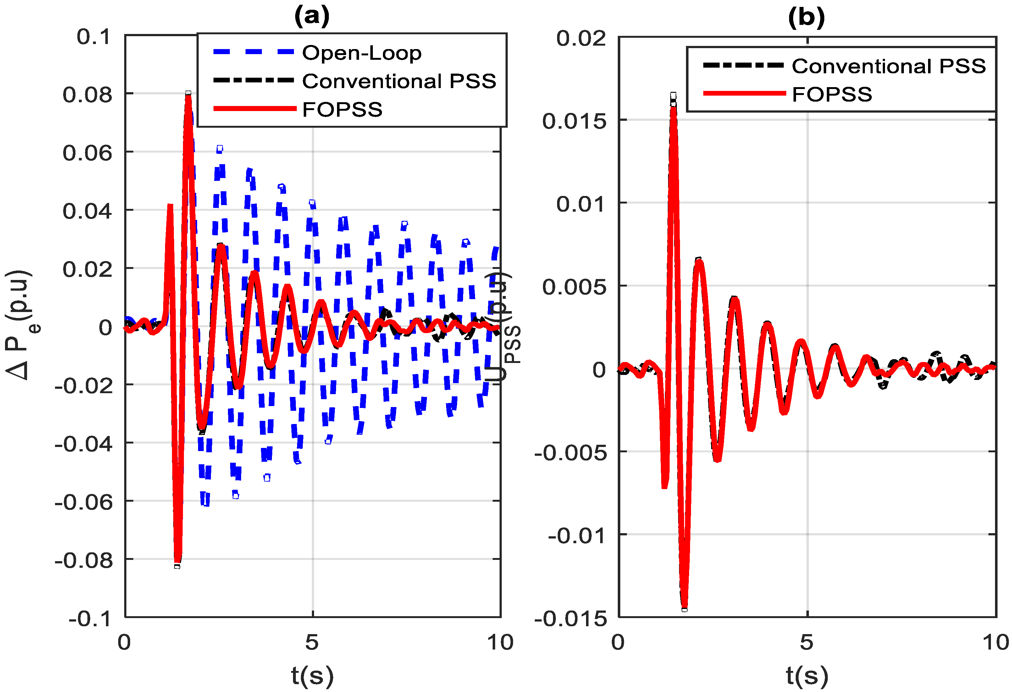
6.2. FOPSS Robust Performance Assessment

By using the inequalities in Equation (24) and (25), the corresponding forbidden regions have been computed for the robust performance assessment of the designed FOPSS controller. In Figure 11, the Bode plot for the designed nominal loop transfer function L0FOPSS(s) = CFOPSS(s)Po(s) is presented.
In Figure 11, the regions in which the robust performance of the closed-loop system is violated (forbidden regions) are indicated by dark and gray colors. It can be observed that, for the range of frequencies of the controller design, namely ω   [1, 100] rad/s, the plot, | L o F O P S S ( j ω ) | = | C F O P S S ( j ω ) P o ( j ω ) | does not intersect the forbidden regions in the considered frequency range. This result confirms that FOPSS is robust against the set of acknowledged operating point dependent uncertainties. In Figure 11, the plot | L o P S S ( j ω ) | = | C P S S ( j ω ) P o ( j ω ) | is also presented, for the designed conventional PSS. The conventional PSS is also robust while showing a lightly reduced robustness margin in comparison to the fractional order PSS.

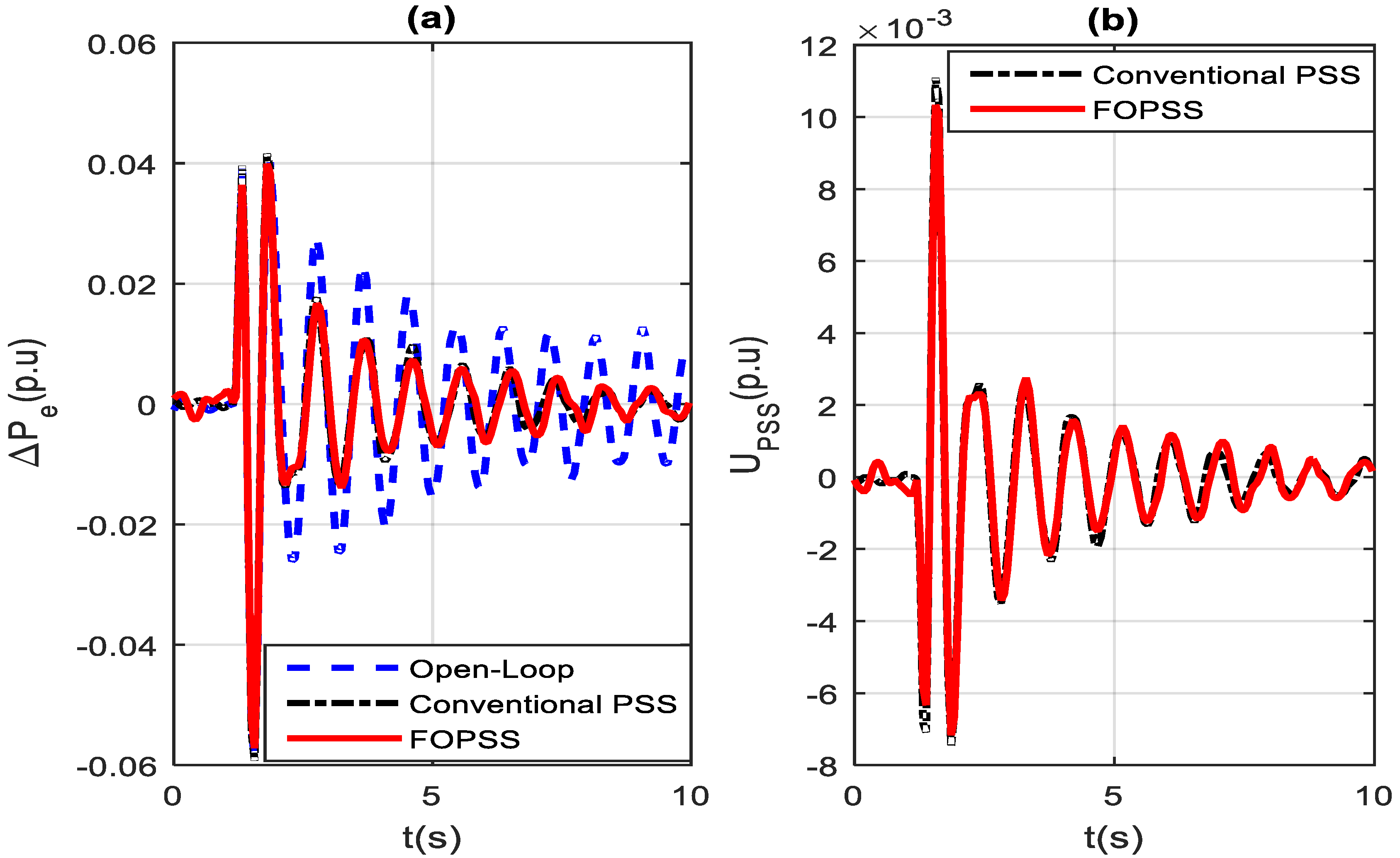
7. Practical Tests Performance Evaluation

7.1. Experimental Field Tests

In this subsection, the results obtained by carrying out experimental tests on the 10 kVA small-scaled power system are presented and discussed. The signal corresponding to open-loop tests (without using any damping controller) are shown in blue color dashed line. For the closed-loop cases, black color dash-dot line is used for the signals corresponding to the conventional PSS performance while red color solid line is used to signals corresponding to the performance of the fractional order PSS (FOPSS).
In Figure 12a, the performance behavior of the active power deviation obtained for a low load level operating condition (active power close to 0.1 p.u.) is shown, while, in Figure 12b, the corresponding control effort is shown. The applied disturbance pulse signal has a short-duration (around 60 ms) and small amplitude (0.05 p.u.). This disturbance test signal was applied in superposition to the setpoint value of the AVR Controller (around 1.0 p.u.). It can be observed in Figure 12a that the FOPSS shows effective damping of the dominant electromechanical oscillation. Furthermore, it can also be observed that this performance is obtained with a control effort lightly reduced in comparison to conventional PSS effort (see Figure 12b).
Figure 13a presents the closed-loop system response for the power system at the high loading operation point 0.6 p.u. The FOPSS performance had almost the same behavior as the previously analyzed operating condition. It can be observed that the FOPSS controller was able to provide effective damping of the oscillations. Figure 13b presents the corresponding controls effort, showing that the FOPSS effort remains lower than the effort provided by the conventional PSS.

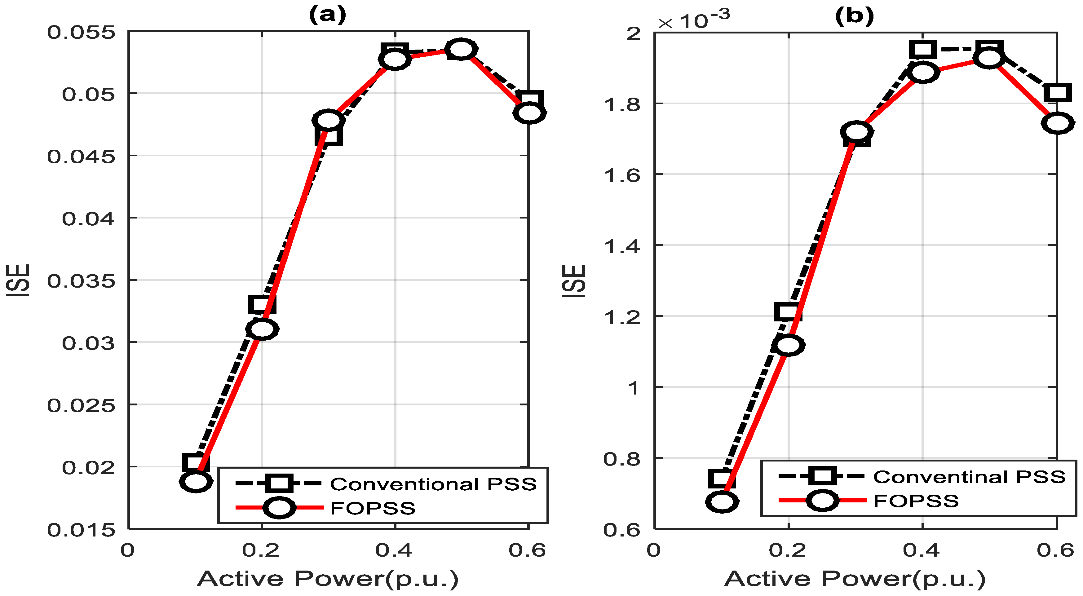
7.2. Cost Function Evaluation

The obtained results were also corroborated by an analysis of the performance indices Integral of Square Error (ISE) calculated from the active power deviation and control signals to six different operation points {0.1, 0.2, 0.3, 0.4, 0.5, 0.6} in the time domain for both PSSs.
I S E = 0 e ( t ) d t .
Figure 14 shows the ISE for all the six investigated operating points related to the active power deviation response (Figure 14a) and the corresponding cost function for control effort (Figure 14b). It can be observed, in Figure 14a, that the ISE value obtained for the FOPSS controller is smaller than the ISE value obtained when applying the conventional PSS controller for most of the tested operating condition, from low to high level of active power generation. In fact, Figure 14a shows that the control effort provided for both (PSS and FOPSS) controllers are quite similar. These results indicate that the FOPSS may be regarded as competitive for real-world applications in large generator units. Figure 14b reveals that the improved performance obtained by the FOPSS is achieved without using an excessive control effort. Figure 14b presents the cost function applied related to the system control signal at all six operation points. At an operating point corresponding to a low level of loading (0.3 p.u), the ISE obtained for the FOPSS controller shows to be slightly above the one obtained for the conventional PSS. This result might be due to some time-variable uncertainties that happen during experimental tests, including variations on the value of the RMS voltage of the larger power system. Thus, FOPSS has an improved dynamic behavior of active power deviation.

8. Conclusions

This paper reportes the design and experimental tests of a fractional order based power system stabilizer (FOPSS). The FOPSS can be seen as a natural extension of the conventional Lead-Lag based PSS structure. In this case, the fractional order parameter provides an additional degree of freedom which may be exploited to obtain performance robustness improvements.
Regarding the damping of the target dominant oscillation mode, it was found, by performing experimental tests in a laboratory scale power system, that the FOPSS presents a reduced loss of performance in comparison to its conventional counterpart, for the set of allowed operating conditions. Furthermore, the improved robustness of the FOPSS has been obtained using a similar control effort to the one provided by using a conventional PSS. The obtained experimental results for the power system studied in this paper shows that the AVR modes (frequency around 16 rad/s) have slightly greater damping than the damping values obtained for the same mode, in comparison to the designed conventional PSS. However, further additional theoretical studies must be performed to affirm that this behavior holds in general case. A possible FOPSS drawback is its more demanding computational implementation which may demand high order digital filters to obtain a suitable approximation of the fractional order dynamics. An advantage of fractional order approach is its ability to provide improved performance due to its additional tuning parameters. However, to the best of the author’s knowledge, this is a challenging problem from a complex analysis domain to which a formal solution remains to be provided. According to Reference [14], thus far, such statement has only been evidenced using practical tests in rig systems. The experimental results presented in the present paper seem to empirically corroborate this statement, as it can be observed that, for the studied power system, the FOPSS provided presented a robust performance with control effort not higher than the control provided by the conventional PSS.

Author Contributions

Conceptualization, Florindo Antonio de Carvalho Ayres Júnior; Data curation, Florindo Antonio de Carvalho Ayres Júnior and Renan Landau Paiva de Medeiros; Formal analysis, Florindo Antonio de Carvalho Ayres Júnior, Renan Landau Paiva de Medeiros and Walter Barra Júnior; Investigation, Florindo Antonio de Carvalho Ayres Júnior and Renan Landau Paiva de Medeiros; Methodology, Florindo Antonio de Carvalho Ayres Júnior; Software, Florindo Antonio de Carvalho Ayres Júnior, Renan Landau Paiva de Medeiros and Walter Barra Júnior; Supervision, Florindo Antonio de Carvalho Ayres Júnior, Marcelo Kaminski Lenzi and Carlos Tavares Costa Júnior; Validation, Florindo Antonio de Carvalho Ayres Júnior, Renan Landau Paiva de Medeiros and Cleonor Crescêncio das Neves; Visualization, Florindo Antonio de Carvalho Ayres Júnior; Writing—original draft, Florindo Antonio de Carvalho Ayres Júnior, Renan Landau Paiva de Medeiros and Cleonor Crescêncio das Neves; and Writing—review and editing, Florindo Antonio de Carvalho Ayres Júnior, Renan Landau Paiva de Medeiros, Walter Barra Júnior, Cleonor Crescêncio das Neves, Marcelo Kaminski Lenzi, Carlos Tavares da Costa Júnior and Gabriela de Mattos Veroneze.

Funding

This research was funded by Coordenação de Aperfeiçoamento de Pessoal de Nível Superior (CAPES), Conselho Nacional de Desenvolvimento Científico e Tecnológico (CNPq), Universidade Federal do Pará (UFPA), Universidade Federal do Amazonas (UFAM), Instituto Federal do Amazonas (IFAM), and Fundação de Amparo à Pesquisa do Amazonas (FAPEAM).

Acknowledgments

The authors acknowledge, for all scientific contributions, the members of the research groups of e-Controls (UFAM), LESF (UFPR) and LACSPOT (UFPA) for development of this research.

Conflicts of Interest

The author declares no conflict of interest.

References

  1. Kundur, P. Power System Stability and Control; McGraw-Hill: Toronto, ON, Canada, 1994; pp. 699–825. [Google Scholar]
  2. Peter, W.S.; Pai, M.A. Power System Dynamics and Stability; Stipes Publishing: Upper Saddle River, NJ, USA, 1998; pp. 221–282. [Google Scholar]
  3. Barreiros, J.A.L.; Silva, A.S.; Costa, J.A.S. A self-tuning generalized predictive power system stabilizer. Electr. Power Energy Syst. 1998, 20, 213–219. [Google Scholar]
  4. Fabrício, G.N.; Walter, B.J.; Carlos, T.C.J.; Anderson, R.B.M.; Marcus, C.M.G; Janio, J.L. Design and Experimental Evaluation Tests of a Takagi-Sugeno Power System Stabilizer. IET. Gener. Trans. Distrib. 2013, 8, 451–462. [Google Scholar]
  5. Gustavo, K.D.; Aguinaldo, S.S. Robust Design of Power System Controllers Based on Optimization of Pseudospectral Functions. IEEE Trans. Power. Syst. 2013, 28, 1756–1765. [Google Scholar]
  6. Concepción, A.M.; Blas, M.V.; Vicente, F.; Yangquan, C. Tuning and Auto-tuning of Fractional Order Controllers for Industry Applications. Control Eng. Pract. 2008, 16, 798–812. [Google Scholar]
  7. Xue, D.; Zhao, C.; Chen, Y. Fractional Order PID Control of DC-Motor with Elastic Shaft: A Case Study. In Proceedings of the 2006 American Control Conference, Minneapolis, MN, USA, 14–16 June 2006; pp. 3182–3187. [Google Scholar]
  8. Ali, A.J.; Shabnam, K. Tuning of FOPID Controller Using Taylor Series Expansion. Int. J. Sci Commer. Eng. Res. 2011, 2, 1–5. [Google Scholar]
  9. Majid, Z.; Masoud, K.G.; Nasser, S.; Mostafa, P. Design of a Fractional Order PID Controller for an AVR Using Particle Swarm Optimization. Control Eng. Pract. 2009, 17, 1380–1387. [Google Scholar]
  10. Mohammad, R.F.; Abbas, N. On Fractional-Order PID Design. Appl. MATLAB Sci. Eng. 2011. [CrossRef]
  11. Riccardo, C.; Giovanni, D.; Luigi, F.; Ivo, P. Fractional Order Systems: Modeling and Control Applications; World scientific: Hackensack, NJ, USA, 2010; pp. 1–30. [Google Scholar]
  12. Larsen, E.V.; Swann, D.A. Applying Power System Stabilizers Part II: Performance Objectives and Tuning Concepts. IEEE Trans. Power Deliv. 1981, PAS-100, 3025–3033. [Google Scholar] [CrossRef]
  13. Duarte, V.; Jose, S.C. An Introduction to Fractional Control; IET: London, UK, 2013; pp. 79–106. [Google Scholar]
  14. Monje, C.A.; Chen, Y.; Vinagre, B.M.; Xue, D.; Feliu-Batlle, V. Fractional Order Control Systems, Fundamentals and Applications; Springer: London, UK, 2010; pp. 133–140. [Google Scholar]
  15. Landau, I.D.; Zito, G. Digital Control Systems: Design, Identification and Implementation; Springer: London, UK, 2006; pp. 201–245. [Google Scholar]
  16. Ayres Junior, F.A.d.C. Controle de Ordem Fracionária Aplicadas ao Amortecimento de Oscilações Eletromecânicas em Sistemas Elétricos de Potência. Master's Thesis, Universidade Federal do Pará, Belém, Brazil, August 2014. [Google Scholar]
  17. Takenori, A.; William, M. Modified Bode Plots for Robust Performance in SISO Systems with Structured and Unstructured Uncertainties. IEEE Trans. Control Syst. Technol. 2012, 20, 356–368. [Google Scholar]
  18. John, C.D.; Bruce, A.F.; Allen, R.T. Feedback Control Theory; Macmillan Publications: New York, NY, USA, 1992. [Google Scholar]
Figure 1. (a) Layout; and (b) control panel developed.
Energies 11 02052 g001
Figure 2. (a) Small-scale 10kVA Power System at UFPA; and (b) equivalent one-line diagram.
Energies 11 02052 g002
Figure 3. AVR and PSS man–machine interface.
Energies 11 02052 g003
Figure 4. Impulse response of active power deviation (MEDIUM loading (Pe = 0.5 p.u)).
Energies 11 02052 g004
Figure 5. Frequency response of active power deviation and PRBS signals.
Energies 11 02052 g005
Figure 6. Measured (dashed line) and the estimated (continuous line) active power deviation response.
Energies 11 02052 g006
Figure 7. Magnitude Bode plot for the identified models P1, P2 and P3.
Energies 11 02052 g007
Figure 8. Flowchart describing the identification methodology.
Energies 11 02052 g008
Figure 9. Flowchart describing the FOPSS design methodology.
Energies 11 02052 g009
Figure 10. Weighting functions W1 and W2: (a) | W 1 ( j ω ) | plot; and (b) | W 2 ( j ω ) | plot.
Energies 11 02052 g010
Figure 11. Bode Plot of L0FOPSS(s) and L0PSS(s).
Energies 11 02052 g011
Figure 12. (a) Active power deviation response; and (b) control effort at 0.1 p.u. operation point.
Energies 11 02052 g012
Figure 13. (a) Active power deviation response; and (b) control effort, at 0.6 p.u. operation point.
Energies 11 02052 g013
Figure 14. Cost function analysis: (a) ISE for output system response; and (b) control effort cost function.
Energies 11 02052 g014
Table 1. Small-scale system generation parameters values
Resistance and Reactance (p.u.)
RaXdXqX’dX’’dX’’q
Values0.0481.0580.6930.1690.07360.0736
Time Constants (s)
T’d0 T’’d0 T’’q0 H
0.4900.0190.0193.861
Table 2. Identified Local Models Parameters, sampling time TS = 0.06 s.
Low Loading
(Pe = 0.3 p.u)
P1
B(q−1) Coefficients Pe = 0.3 p.u.
b1b2b3b4
0.0122760.143705−0.075265−0.111931
A(q−1) Coefficients Pe = 0.3 p.u.
a1a2a3a4
−2.586840 3.020355 −1.832865 0.555510
Medium loading
(Pe = 0.5 p.u)
P2
B(q−1) Coefficients Pe = 0.5 p.u.
b1b2b3b4
0.019359 0.152224 -0.085471 -0.117924
A(q−1) Coefficients Pe = 0.5 p.u.
a1a2a3a4
−2.5858563.014485−1.8199590.550024
High loading
(Pe = 0.65 p.u)
P3
B(q−1) Coefficients Pe = 0.65 p.u.
b1b2b3b4
0.017439 0.132755 −0.039632 −0.134924
A(q−1) Coefficients Pe = 0.65 p.u.
a1a2a3a4
−2.4859722.763681−1.5905660.474089
Table 3. Relative Damping and Natural Frequencies for Eigenvalues of the Identified Local Models.
EigenvalueLocal Model P1Local Model P2Local Model P3
λ1ξ1 = 0.072, ω1 = 7.93 rad/sξ2 = 0.063, ω2 = 8.03 rad/sξ3 = 0.071, ω3 = 8.01 rad/s
λ2ξ1 = 0.072, ω1 = 7.93 rad/sξ2 = 0.063, ω2 = 8.03 rad/sξ3 = 0.071, ω3 = 8.01 rad/s
λ3ξ1 = 0.258, ω1 = 16.80 rad/sξ2 = 0.267, ω2 = 16.80 rad/sξ3 = 0.321, ω3 = 17.60 rad/s
λ4ξ1 = 0.258, ω1 = 16.80 rad/sξ2 = 0.267, ω2 = 16.80 rad/sξ3 = 0.321, ω3 = 17.60 rad/s
Table 4. Parameters values for the designed FOPSS and Conventional PSS.
Parameters ValuesConventional PSS
KPSST1T2N
0.28490.2000 s0.2556 s2
FOPSS
KPSST1T2α
0.24290.2000s0.0783 s−0.4587
Table 5. Eigenvalues of the nominal closed-loop system poles
Pole 1Pole 2Pole 3Pole 4Pole 5Pole 6
Classic PSS eigenvalues (rad/s)3.384.198.548.5415.915.9
Relative damping ξ1.01.00.1830.1830.2250.225
FOPSS Eigenvalues (rad/s)5.358.578.579.7315.915.9
Relative damping ξ1.00.1850.1851.00.2310.231
Table 6. Parameters values for the digital form of PSS and FOPSS, sampling time TS = 0.06 s.
ParametersPSSFOPSS
r00.18500.1721
r1−0.2718−0.1902
r20.09980.0513
s1−1.5724−1.2407
s20.61810.3777

