The Synergies of Shared Autonomous Electric Vehicles with Renewable Energy in a Virtual Power Plant and Microgrid

Abstract

The introduction of shared autonomous electric vehicles (SAEVs), expected within the next decade, can transform the car into a service, accelerate electrification of the transport sector, and allow for large scale control of electric vehicle charging. In this work, we investigate the potential for this system to provide aggregated storage when combined with intermittent renewable energy sources. We develop a simulation methodology for the optimization of vehicle charging in the context of a virtual power plant or microgrid, with and without grid connection or distributed dispatchable generators. The model considers aggregate storage availability from vehicles based on transport patterns taking into account the necessary vehicle redistribution. We investigate the case of a grid-connected VPP with rooftop solar and the case of a isolated microgrid with solar, wind, and dispatchable generation. We conduct a comprehensive sensitivity analysis to study the effect of several parameters on the results for both cases.

1. Introduction

New transport paradigms have been emerging in recent years thanks to the widespread use of connected devices. This is leading to a shift from car ownership to car sharing models of transportation. One-way car sharing services, in which passengers rent a vehicle by the minute wherever it is currently parked and leave it at any other place within a given area, are already common in large cities in Europe [1]. Autonomous driving technology would allow vehicles to autonomously move to passengers when called, making shared transportation much more convenient and speeding up its adoption [2].

The introduction of shared autonomous electric vehicles (SAEVs), or robot taxis as they are sometimes referred to, will also transform the transport sector from the perspective of energy use. SAEVs may be an important enabler of transport sector electrification [3]. It is therefore important to study the impact of this system on the electricity grid. In particular, SAEVs can offer synergies in the framework of a Virtual Power Plant (VPP) or microgrid. Users may sign up for both electricity and transport services from the same provider (the VPP/microgrid and SAEV operator), avoiding the costs of owning a private car. This scheme may lower the total costs of the system and may allow a larger penetration of renewable energy in the grid.

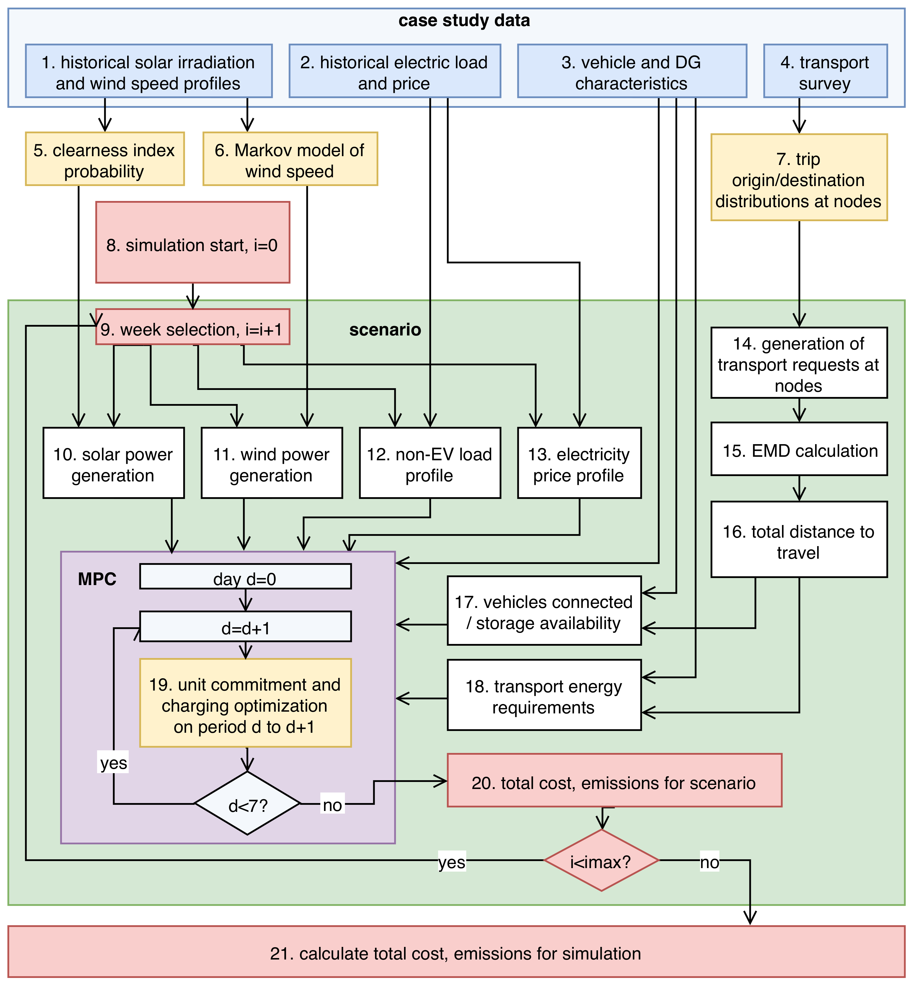
Most studies on the charging of electric vehicles and their interaction with renewable energy have focused on private vehicles, mostly assuming that vehicles are used once or twice a day and charged at night [4]. In this work, we present a methodology for the optimization of SAEVs charging with distributed dispatchable generators (DG), renewable energy generators, grid electricity with variable pricing, vehicle-to-grid, and considering vehicles’ rebalancing requirements. We investigate the costs and carbon emissions of a SAEV system in the context of a grid-connected VPP and of an isolated microgrid compared to alternative energy storage and transport options. The economic performance of SAEVs would improve in the case of larger fluctuating renewable energy penetration. This is considered to be a synergy effect of SAEVs and renewable energy. Therefore, the aim of this study was to evaluate this synergy effect quantitatively by using the proposed method for optimizing the charging of SAEVs.

The work is organized as follows. In Section 2, we present an overview of the related work in this field. In Section 3, we introduce the methodology used, including the transport demand generation, the charging optimization algorithm, and the renewable energy profile generation. In Section 4, the assumptions and methodology specific to our case studies are presented. In Section 5, we report and discuss the results of the simulations for the case study. In Section 6, we present our conclusions and future work.

2. Related Work

The related academic work in this field mainly concerns the integration of renewable energy with electric vehicles and their synergies, and the operation of shared autonomous electric vehicles. There is a vast literature on the interaction of private EVs with renewable energy, and many studies have focused on SAEV operation. Electric vehicles offer great opportunities for grid balancing and integration of renewable energy sources, because of the flexibility of charging [5,6]. Vehicle to grid (V2G), or the discharge of vehicle batteries to the grid, has also been proposed as a way to further increasing their benefits by replacing peak generation [7,8]. Effective strategies have been developed for the participation of aggregated vehicle fleets with V2G in the electricity markets [9].

Most studies on electric vehicles and renewable energy consider private vehicles. Liu et al. [6] presented a review of electric vehicles interacting with renewable energy in the context of the smart grid. They categorized work on EVs into three types depending on the objective: minimization of cost, maximization of efficiency or minimization of emissions. The review also highlights that mixed-integer linear programming (MILP) and stochastic analysis for intermittent renewable energy sources are common in the literature. Liang and Zhuang [10] discussed the literature on stochastic modeling and optimization in microgrids. Nosratabadi et al. [11] presented a useful review of distributed energy scheduling in microgrid and virtual power plants, including work that consider EVs. Mwasilu et al. [12] presented a review of the work on the interaction between EVs with V2G and renewable energy. One of the highlighted problems is the difficulty in implementing V2G in practice with private vehicles.

Wang et al. [13] studied the impact of electric vehicles and demand response on a power system with wind power generation. The simulations are run over a the period of a week, with 24 h optimization period and the last hour of the previous period used as the first hour of the next optimization period. They modeled the availability of vehicles by estimating the time of arrival of the vehicle at home. They found that electric vehicles can significantly decrease the cost when smart charging of vehicles is employed for the case study of the expected Illinois grid in 2020. Su et al. [14] proposed a stochastic optimization model for operating cost minimization of a microgrid with EVs, wind and solar power, batteries, and distributed dispatchable generators. They considered both the energy scheduling problem and subsequently iteratively adjusted the results to minimize distribution losses and satisfy grid constraints. Saber and Venayagamoorthy [15] proposed a method to maximize renewable energy utilization to minimize costs and emissions in smart grid with EVs and V2G. Schuller et al. [16] formulated a MILP problem for the quantification of load flexibility of EVs for renewable energy integration in the grid. They used driving patterns of full-time employees and retired persons from the German Mobility Panel to simulate two common classes of vehicle usage. Renewable generation is taken from the German grid and scaled to the actual consumption of EVs to quantify the ability of EVs to balance the intermittent generation. They considered backup generators in form of gas turbines. The study analyzes the effect of shorter optimization horizon from a week to one day to test a more realistic limited advanced knowledge. They concluded that optimal smart charging significantly increases the utilization of renewable energy, with the best performance in a solar/wind mixed generation portfolio. They also found that EVs have significant inter-day flexibility. Arslan and Karasan [17] developed an energy management model for the minimization of VPP costs considering distributed generation, renewable energy sources, and EVs. They evaluated the impact of VPP formation on costs and carbon emissions in a community. They conducted a extensive sensitivity analysis to understand the influence of several parameters on the results for a case study in California. They concluded that VPP are effective at decreasing costs for participants and can represent a solution to several challenges in the electricity market in the future.

Vehicle connection is one of the main problems for coordinating the charging of private electric vehicles [18,19]. This has been generally dealt with by estimating the time of arrival of people at home [13,18,19,20]. Another problem is the determination of the minimum final SOC of private vehicles. Many studies assume that vehicles should have 100% SOC at the beginning of the day [13,21], thus limiting the amount of charging flexibility allowed. These problems are mitigated by SAEVs, as vehicles can move to charging stations whenever they are not transporting passengers.

There is limited literature focusing on shared EV systems. Kahlen and Ketter [22] developed an algorithm for the control of vehicles in a carsharing system. Decisions in this model concern the commitment of vehicles for operating reserve, the charging of vehicles, or the commitment for transport service. The decision is made by comparing expected profits over future time steps for each action, and it is calculated with a multiple linear regression model. By testing the model with data from a free floating carsharing system they found that profits could increase by 7–12% with practically no decrease in vehicle availability. Biondi et al. [23] developed a method for the optimal positioning of charging station for electric car sharing systems and study the impact of these systems on the electricity grid.

SAEV operations in terms of transport have been the focus of several studies. Zhang et al. [24] developed a model predictive control approach for the optimization of an autonomous car-sharing system with rebalancing which considers electric charging constraints. Chen et al. [25] studied the operation of a SAEV system with a model based on Ref. [2]. The agent-based transport model methodology is similar, but the investigation is expanded by including charging of the electric vehicles serving 10% of trip demand in a medium-sized metropolitan area. Bauer et al. [26] developed an agent-based model for the simulation of SAEV. They found the optimal battery size and number of charging stations to minimize costs through sensitivity analysis. They concluded that vehicles with 50–90 miles range and 66 chargers per square mile (25 per square km) with a 11 kW connection can provide service with a cost of $0.29–$0.61 per mile ($0.18–$0.38 per km), about 10 times lower than normal taxis and lower than if the service was provided by any non-electric vehicle. They also calculate that SAEVs would reduce GHG emissions by 73% compared to current taxis with the current power grid. Chen et al. [27] introduced a methodology for the optimal routing and charging of EVs in a fleet. They included a simplified analysis of the possible impacts of the system on the electricity distribution network. All models considered do not consider “smart” charging, or optimized charging taking into consideration grid-side aspects such as dynamic electricity price or grid constraints. In particular, Chen et al. [25] found that simultaneous charging of the fleet at peak times may be problematic for the electric grid. This is a known problem of uncoordinated electric vehicles charging [7].

As shown in this section, the topic of shared vehicles interacting with renewable energy has been largely overlooked. SAEVs present different availability patterns compared to private vehicles. Private vehicles tend to be connected at night and less during the day while owners stay at their destination. In contrast, SAEVs can be connected at any time when they are not serving passengers. Moreover, SAEVs have the potential to replace a large number of vehicles, thus decreasing the total amount of battery storage available. As many studies on SAEVs predict that these systems will soon be commercially available and potentially replace private vehicles in many cases, it is important to understand the impact of this shift on the potential for electrified transportation to integrate renewable energy in the grid.

3. Methods

A mixed-integer linear optimization model is used to schedule the optimal charging and discharging of the aggregate fleet of SAEVs to minimize total costs for the VPP or microgrid. Transport demand, base load (non-EV) and renewable energy generation are considered external inputs. Transport demand and renewable energy generation profiles are generated stochastically based on transport survey and historical weather data, respectively. A simplified diagram of the model flow is shown in Figure 1, while the nomenclature used is summarized in

Table 1. Nomenclature.

Symbol	Description
A. Indices and simulation variables
$c\left(t\right),q\left(t\right)$	Charge energy and V2G discharge energy
$d_{i,j}$	distance between node i and j
$e\left(t\right)$	Energy stored in vehicles
$e_{max}\left(t\right)$	Maximum energy exchangeable
$f_{pass}\left(t\right)$	Distance for passenger trips
$f_{rel}\left(t\right)$	Distance for rebalancing
$f_{tot}\left(t\right)$	Total distance
$g_j\left(t\right)$	Generation from DG
$o_j\left(t\right)$	DG operation binary variable
$i\left(t\right),k\left(t\right)$	Energy imports and exports
$L\left(t\right)$	Non-EV electricity load
$m_{av}\left(t\right)$	Vehicles available
$P_w\left(t\right),P_s\left(t\right)$	Wind and solar generation
t	Time step
$v_j\left(t\right),w_j\left(t\right)$	DG start-up and shut-down binary variables
$\lambda \left(t\right)$	Rate of Poisson process
B. Parameters and constants
$C_{battery}$	Cost of battery (yen/kWh)
$C_{car}$	Cost of car (with no battery)
$C_{startup}$	Start-up cost
$CAP$	Battery capacity (kWh)
$EC$	Electricity consumption of cars (kWh/km)
$e_{v,max}$	Maximum energy exchangeable per vehicle (kWh/km)
$i_{max}$	Maximum power exchangeable with grid (kW)
$L_{battery}$	Life of battery in equivalent full cycles
$L_{car}$	Life of car not including battery (years)
m	Total number of vehicles
$P_{cap,w},P_{cap,s}$	Wind and solar installed capacity
$u\left(t\right)$	Average speed of vehicles (km/time step)
$y\left(t\right)$	Electricity price (yen/kWh)
$z_{i,j}$	Markov transition probability between state i and j
$\beta$	Ratio of trip distance to Euclidean distance
$\eta$	Battery round-trip efficiency
C. Acronyms
DG	Distributed generation
EMD	Earth Mover’s distance
SAEV	Shared autonomous electric vehicle
SOC	State of charge
V2G	Vehicle to grid

.

3.1. Transport Demand Generation

The transport demand is based on transport survey data (block 4 in Figure 1). The total number of passengers at each time interval t is determined stochastically with a Poisson process with rate $\lambda \left(t\right)$ dependent on the relative frequency of trips at that time of day and the average trips per hour of the simulation (block 14 in Figure 1). The scaling of the simulation is determined by the average trips per day (TPD) or average trip rate.

Each passenger request is generated at a specific node of the simulation, which is extracted from the trip origin and destination node distributions for the specific time of day. The generated trips are stored in matrix $A\left(t\right)$, where $a_{ij}$ is the number of passengers originating from node i with destination node j. The distance between each node and each other node is stored in the symmetric square matrix D, where each element $d_{ij}$ is the distance between node i and node j. The values are calculated from the Euclidean distance between nodes multiplied by an average tortuosity factor to account for the street layout. The total distance traveled to transport passengers can therefore be expressed as:

$$f_{pass}\left(t\right)=\sum _j\sum _i{a}_{ij}\left(t\right)·d_{ij}$$

(1)

Passenger origin and destination distributions are typically not symmetric during any period of time shorter than a day. Vehicles would therefore tend to accumulate at certain nodes with higher destination rates and would be unavailable at nodes with high origin rates. To ensure service to all passengers, redistribution of vehicles is needed. It has been shown that the minimum amount of additional distance to travel for redistribution is equivalent to the Earth Mover’s Distance (EMD) between the origin and destination distributions during a certain period of time [28]. This is also known as Wasserstein or Kantorovich distance. The EMD is a theoretical minimum rebalancing distance, which can however be reached in practice with an efficient routing strategy [28]. For the purpose of this work, the EMD is calculated for each time interval from the trip distributions using the algorithm in [29] (block 15 in Figure 1). This extra relocation travel distance $f_{rel}\left(t\right)$ is added to the total distance traveled for trips with passengers to account for the energy needed for rebalancing (block 16 in Figure 1). An example of the results is shown in Figure 2a.

The model assumes that the distribution of trips within a time period is uniform. In addition, the position of electricity load and injections in the grid is not considered, since the actual position of specific vehicles is not simulated.

3.2. Unit Commitment and Charging Optimization

In this section, the charging optimization model is described (block 19 in Figure 1). The total energy stored in the vehicles e evolves as:

$$e(t+1)=e\left(t\right)-d\left(t\right)+c\left(t\right)-q\left(t\right)/\eta$$

(2)

where d, c, and q are, respectively, transport energy demand, charge, and V2G discharge during time t, all non-negative. $\eta$ is the efficiency of V2G, set at 0.9. $q=0$ for simulations without V2G. The electricity flow balance is stated as:

$$P_w\left(t\right)+P_s\left(t\right)-L\left(t\right)+i\left(t\right)-k\left(t\right)-c\left(t\right)+q\left(t\right)+\sum _j{g}_j\left(t\right)\ge 0$$

(3)

where $P_w$ and $P_s$ are the wind and solar power generation, L is non-EV electric load in the system, i is the grid import, k is the grid export, and $g_j$ is the generation from unit j.

The dispatchable distributed generators (DG) units are controlled with three binary decision variables, $v_j\left(t\right)$, $w_j\left(t\right)$, $o_j\left(t\right)$, to account, respectively, for start-up, shutdown and operation of generator j at time t. The constraints for the generators are:

$$o_j\left(t\right)-o_j(t-1)=v_j\left(t\right)-w_j\left(t\right)$$

(4)

$$g_{j,min}·o_j\left(t\right)\le g_j\left(t\right)\le g_{j,max}·o_j\left(t\right)$$

(5)

$$v_j\left(t\right),w_j\left(t\right),o_j\left(t\right)\in \{0,1\}$$

(6)

with $g_{j,min}$ and $g_{j,max}$, respectively, the minimum and maximum generation for generator j when operational. The grid import/export capacity should also be less than the maximum capacity $i_{max}$:

$$0\le i\left(t\right)\le i_{max}$$

(7)

$$0\le k\left(t\right)\le i_{max}$$

(8)

The energy stored is constrained by the battery capacity of vehicles and the initial energy stored at the beginning and at the end of the time period:

$$e\left(0\right)=CAP·m·SO{C}_0$$

(9)

$$CAP·m·SO{C}_{min}\le e\left(t\right)\le CAP·m$$

(10)

$$e\left(t_{end}\right)\ge CAP·m·SO{C}_{end}$$

(11)

with $CAP$ the battery capacity of each vehicle, m the number of vehicles, $SO{C}_{min}$ the minimum state of charge of the combined fleet, and $SO{C}_0$ and $SO{C}_{end}$, respectively, the initial SOC and the minimum final SOC at the end of the period.

The amount of energy that can be charged or discharged from vehicles during a time interval is constrained by the number of vehicles connected to a charging station during the interval (block 17 in Figure 1). Assuming a uniform distribution of passenger trip requests during the period, the average number of vehicles connected is:

$$m_{av}\left(t\right)=m-\frac{f_{pass}\left(t\right)+f_{rel}\left(t\right)}{u\left(t\right)·t_{len}}$$

(12)

where u is the average speed of vehicles and $t_{len}$ is the length of the time step interval. The maximum energy exchangeable is therefore:

$$e_{max}\left(t\right)=m_{av}\left(t\right)·e_{v,max}$$

(13)

$$0\le c\left(t\right)\le e_{max}\left(t\right)$$

(14)

$$0\le q\left(t\right)\le e_{max}\left(t\right)$$

(15)

where $e_{v,max}$ is the maximum energy that can be exchanged by each vehicle during a time interval. This is a function of the choice of power connection and the length of the interval. The actual instantaneous power exchangeable during the period may vary depending on the specific position of vehicles. In this work, we assume that the power connections allow for higher power levels if required.

The model objective is the minimization of total cost. This includes costs from the grid, from the generators, and the cost of battery cycling. The cost function for the grid interaction is:

$$C_{grid}\left(t\right)=i\left(t\right)·y\left(t\right)-k\left(t\right)·y\left(t\right)·{\eta }_{grid}$$

(16)

$y\left(t\right)$ is the price of electricity from the grid at time t, and ${\eta }_{grid}$ is an efficiency parameter representing the cost of selling to the grid and to avoid simultaneous import and export. This was chosen as 0.99. The cost function for DG considers the start-up costs and cost of generation:

$$C_{DG}\left(t\right)=\sum _j\left(i_j\left(t\right)·C_{op,j}+v_j\left(t\right)·C_{start,j}\right)$$

(17)

The objective function is therefore:

$$min\sum _t\left(C_{grid}\left(t\right)+C_{DG}\left(t\right)+\frac{{\gamma }_{cycles}·c\left(t\right)·C_{bat}}{L_{bat}}\right)$$

(18)

subject to the constraints listed above. ${\gamma }_{cycles}$ is the fraction of the battery costs amortized by cycling as opposed to aging, which was chosen as 0.5 (see also Section 4.4). The model presented can be solved with mixed integer linear programming methods.

3.3. Renewable Energy Generation

Renewable energy generation profiles for wind and solar power were generated stochastically based on historical data. Load, solar, and wind profiles were assumed to be independent.

Wind speed profiles were generated with a Markov model based on historical wind speed observation (block 6 in Figure 1). Markov models are often used to generate wind speed profiles based on historical data [30]. Each element of the Markov transition probability matrix Z was determined as:

$$z_{i,j}=\frac{w_{i,j}}{{\sum }_{i}n{w}_{i,j}}$$

(19)

where $n{w}_{i,j}$ is the number of transitions from state i to state j in the historical data, where each state corresponds to a range of wind speeds, discretized into 20 states. The wind power generation $P_w\left(t\right)$ is then calculated considering the wind turbine characteristic curve, which was linearized for simplicity:

$$P_w\left(t\right)=\left\{\begin{array}{cc}{P}_{cap,w}·min(1,max(0,\frac{W\left(t\right)-W_{cutin}}{W_{rated}-W_{cutin}}))\hfill & ifW\le W_{cutoff}\hfill \\ 0\hfill & ifW>W_{cutoff}\hfill \end{array}\right.$$

(20)

where $W\left(t\right)$ is the wind speed.

Solar irradiance profiles were generated from hourly extraterrestrial solar irradiation profiles for the simulation days and location and a stochastically generated average daily clearness index K (block 5 in Figure 1). The probability distribution of K was calculated by comparing computed values for the maximum daily extraterrestrial solar irradiation over actual measured historical irradiation values for each day. Extraterrestrial irradiation was calculated based on methodology reported in the HOMER software documentation [31]. Although solar power generation also varies with the temperature of the panels and other environmental factors, for simplicity in this work the solar power generation $P_s\left(t\right)$ was considered a linear function of the solar irradiance, as an accurate estimation of solar PV generation is outside of the scope of this paper. The maximum PV output was assumed at 1 kW/m${}^2$:

$$P_s\left(t\right)=P_{cap,s}I\left(t\right)/1000$$

(21)

with $P_{cap,s}$ the total solar installed capacity and $I\left(t\right)$ the solar irradiance on the tilted surface at time t in W/m${}^2$. It should be noted that the area of the panels and their efficiency are not considered in this formulation, and we directly calculate the relative hourly capacity factor as a function of solar irradiance.

3.4. Stochastic Simulation

The stochastic simulation evolves as follows. At the start of a simulation (block 8 in Figure 1), a specific week of the year is selected (block 9 in Figure 1). The corresponding weekly profile of non-EV load and price profile is then selected (blocks 12 and 13 in Figure 1), and weather patterns are generated, considering the time of the year (blocks 10 and 11 in Figure 1). The load, price and weather patterns are selected as the scenario for the simulation.

To simulate limited advance knowledge, we assume that the optimization model can only see a portion of the scenario at a time (optimization horizon). A model predictive control (MPC) approach (also known as receding horizon control) was used in the simulations to account for the limited practical prediction horizons for weather patterns and transport demand (see also Figure 1). This allows us to obtain results from optimization based on realistic prediction horizons, while still allowing us to study the behavior of the system over long simulation periods. We used an optimization horizon of two days, thus 48 time intervals are considered when the length of the time interval t is set to 1 h. At each step of the MPC, only the results of the first day of the optimization are considered (first 24 h). The optimization is rerun with an updated optimization period for the next day. In this way, the optimization is run seven times (once for each day, with advance knowledge of the next day) to simulate a whole week. For more accurate results but slower simulation times, the optimization can be run at each hour with only the first hour implemented.

At the end of the simulated week, costs and emissions for the scenario are calculated (block 20 in Figure 1), and the process is repeated with another week until the desired number of iterations are reached. At the end of the simulation, the total costs and emissions for all scenarios (weeks) simulated are averaged to find the results of the simulation (block 21 in Figure 1).

4. Numerical Simulations

The model was developed in MATLAB and tested with a case study in Tokyo.

4.1. Transport Data

The transport request probability is based on the Tokyo Person Trip Survey 2008 [32], a survey of about 2 million trips in the Tokyo metropolitan area. Trips by car in a central 20 km × 20 km area of Tokyo were considered for this work. This area includes about 300 nodes (origin and destination points) shown in Figure 3. More information about the survey extraction methodology and determination of the trip origin/destination distributions (block 7 in Figure 1) can be found in [33].

4.2. Electricity Load and Price

The electricity load profile (block 2 in Figure 1) was taken from the Tokyo Electric Power Company (TEPCO) [34]. Data for the year 2017 were used in the simulations. The electricity load profile was normalized to a daily electricity consumption of 6.3 kWh per person, the average for Japanese residential consumers [35]. We assume that the VPP has access to the wholesale electricity market as a price-taker. This is justified by the scale of the VPP relative to the total electricity market.

The electricity price was taken from the Japan Electric Power Exchange (JEPX) historical day-ahead trading data for the corresponding electricity load in 2017.

4.3. Renewable Generation Data

Hourly solar irradiation data (block 1 in Figure 1) was taken from the Japan Meteorological Agency for Tsukuba weather station (near Tokyo) in the years 2011–2015 [36]. We consider solar panels with tilt equal to the latitude (${36}^{°}$) and peak generation at 1 kW/m${}^2$, resulting in an average yearly capacity factor of 13%. (An example of a solar profile over a week is shown in Figure 2b).

Wind model data was based on 6 years of historical observations from 2010 to 2015 at Tokyo Haneda Airport, taken from NOAA [37] (block 2 in Figure 1). We used a hypothetical typical wind turbine with cut-in speed of 4 m/s, rated speed of 12 m/s and cut-off speed of 25 m/s, resulting in an average yearly capacity factor of 21% with the considered wind speed profile. An example weekly profile is shown in Figure 2b. The generation capacity was sized to generate the total base load (non-EV) electricity consumption over a year. For simulation with solar power only, this is equivalent to about 2 kW of solar PV per person, which is consistent with a rooftop solar PV system size.

4.4. Technical Parameters, Cost, and Emissions Assumptions

This section describes the assumptions related to vehicle and DG characteristics, costs and emissions (block 3 in Figure 1). The exchange rate used in this work was 1 USD = 100 JPY (similar to the current exchange rate as of April 2018). Battery costs were estimated at $200/kWh [40], with a cycle life of 1500 cycles. Costs of the battery were divided in equal parts between amortization costs (calculated over five years) and cycling costs, thus reflecting the practical life of batteries and avoiding underestimating costs of underused storage. Life-cycle emissions of batteries were also included at 50 kg CO${}_2$/kWh capacity, similar to lithium-ion batteries manufactured in the United States [41].

The private vehicle for comparison was assumed to be a hybrid electric vehicle (HEV) with a high fuel efficiency of 23 km/L, similar to those of the 2016 Toyota Prius in city driving [42]. This value is conservative, as it is considerably higher than current average new vehicle efficiency in Japan and higher than the 2020 target for new vehicles of 20.3 km/L [43]. Gasoline prices were assumed at 150 yen/liter. The cost of the vehicle was taken as 2 million yen or $20,000 with a life expectancy of 12 years, the current average for new vehicles in Japan [43]. Emissions from gasoline consumption is 2.3 kg CO${}_2$/liter.

Autonomous vehicle costs (excluding battery) were conservatively estimated at 5 million yen or $50,000 with a life expectancy of five years. This is supported by literature putting the extra price of fully autonomous technology at about $10,000 [44,45]. The extra cost was assumed to be necessary due to the heavier usage of the vehicle compared to a private car, and by the extra cost of maintenance and other expenses which is assumed included in the capital cost. The vehicles’ battery capacity was set at 50 kWh and the maximum power exchange (charging or discharging) at 10 kW. A summary of the transport cost assumptions can be found in

Table 2. Transport mode characteristics.

Characteristic	HEV	SAEV
capital cost	2 million yen	5 million yen
consumption	4.3 L/100 km	0.15 kWh/km
expected life	12 years	5 years

. Grid emission intensity was set at 0.452 kg CO${}_2$/kWh, the average between the value for the Japanese electricity supply in 2015 (0.534) and the 2030 target (0.37) [46]. Renewable energy costs, operation and maintenance costs, payback periods, capacity factors and emissions are summarized in

Table 3. Summary of renewable energy characteristics.

Characteristic	Solar	Wind	Ref.
capital cost (million yen/kW)	0.25	0.20	[38]
O&M cost (yen/kW/year)	0	7600	[38]
payback (years)	10	10	-
capacity factor (%)	13	21	-
emissions (kg CO${}_2$/kWh)	0.041	0.011	[39]

.

As of 2018, Japan had a residential solar feed-in tariff of 26 yen/kWh [47]. High feed-in tariffs in recent years have caused a sharp increase in photovoltaic installations in the country with about 50 GW of cumulative installation at the end of 2017, a 10-fold increase from 2011. It is expected that the feed-in tariff will be progressively decreased and phased out in the coming years to favour self-consumption [48]. In this work, we assume that excess PV power is bought at the price of electricity in the wholesale electricity market (marginal cost of generation). The price of electricity for households was set at 20 yen/kWh, which is close to the average price for TEPCO.

For the microgrid case, hypothetical DG units representing a gas turbine, a diesel generator, and biomass steam plant were used.

Table 4. Summary of distributed generation characteristics including minimum and maximum generation capacity, cost per kWh, and carbon emissions.

DG unit	Min. (kW)	Max. (kW)	Cost (yen/kWh)	CO${}_2$ (kg/kWh)
gas turbine	2000	5000	20	0.6
diesel engine	100	1000	25	0.65
biomass	1000	2000	15	0.4

presents a summary of the characteristics of these units. Approximate values were taken from [49]. Start-up costs for each unit were chosen as the cost of running the unit at full power for one hour.

4.5. Simulation Parameters and Scale

The time interval length for the simulations presented was set to 1 h and the tortuosity factor of roads was set to 1.5 [33]. The fleet size was selected at 1.4 vehicles per average trip per hour (TPH). This ratio was found in previous work to be a good compromise between minimizing waiting times and operating costs of the system [33]. Assuming an average of two trips per private vehicle per day, this suggests that autonomous vehicles would replace traditional vehicles with a proportion of about 1:8.6, in accordance with previous studies [2,44]. The total population assumed in these simulation was chosen as 12,000 people, resulting in a total of 24,000 trips per day (1000 trips per hour average).

5. Results and Discussion

In this study, two cases were considered for analysis: grid-connected VPP without DG, and isolated microgrid with DG. Each data point represents 100 week-long simulations, taken from Mondays to Sundays of the load profile.

5.1. VPP Case

We considered five scenarios to compare the cost and emissions performance of SAEV to other options and the effectiveness of the optimization algorithm in the context of a VPP. These are summarized in

Table 5. Summary of scenarios. VPP does not apply to the microgrid case.

Scenario	Trans-Port	Storage	Charge Sched.	V2G	VPP	RE
BAU	HEV	×	×	×	×	◯
Battery	HEV	◯	◯	×	◯	◯
SAEV1	SAEV	◯	×	×	◯	◯
SAEV2	SAEV	◯	◯	×	◯	◯
SAEV3	SAEV	◯	◯	◯	◯	◯

. The Business as usual (BAU) case assumed private vehicles and electricity from utility at a fixed price of 20 yen/kWh and excess generation sold at the marginal price (see Section 4.4). The battery case assumes that households install a battery and join a VPP with an energy management system that minimizes total costs. The three SAEV scenarios assume that households join a VPP that also provides transport services via SAEV (thus, they avoid buying a private vehicle) without installing a battery. The three scenarios differ with regard to the charging strategy applied, and correspond, respectively, to unscheduled charging, optimized charging without V2G, and optimized charging with V2G.

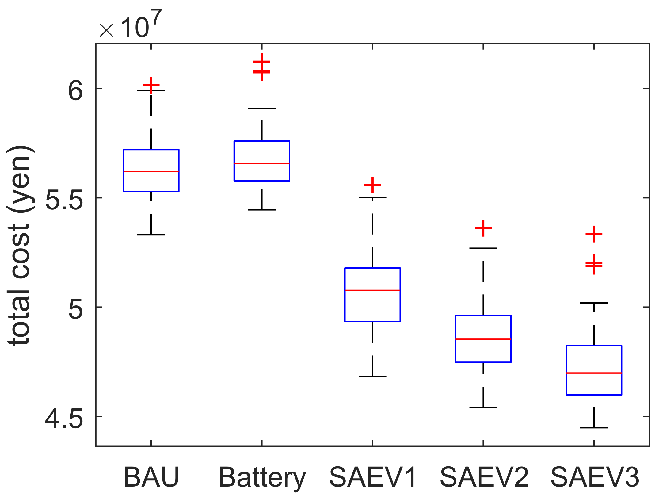
Total costs for each scenario are shown in Figure 4. A breakdown of costs and the CO${}_2$ emissions for each scenario are reported in

Table 6. Costs and emissions for VPP scenarios. Capital includes the cost of vehicles and solar panels.

Scenario	Costs (Million Yen)					CO${}_2$(t)
	Ele.	Fuel	Batt.	Capital	Total
BAU	3.60	3.29	0.00	49.94	56.83	86.7
Battery	−0.99	3.29	3.35	49.94	55.59	94.6
SAEV1	2.17	0.00	3.96	38.44	44.57	129.2
SAEV2	1.47	0.00	3.90	38.44	43.80	124.2
SAEV3	0.77	0.00	4.30	38.44	43.51	128.9

. The cases with transport provided by SAEV (Scenarios 4–6) are the lowest cost options. The cost savings are dominated by capital costs, as vehicles are shared among all participants in the VPP while avoiding the cost of each individual buying a private vehicle. However, the cost of electricity becomes significantly higher in the case of SAEV, although it is still lower than the fuel costs it replaces. The proposed algorithm decreases electricity costs by 32% and 75%, respectively, for the scenario with no V2G and with V2G over the unscheduled charging. The difference would increase with more variable electricity prices in markets with higher penetration of intermittent sources.

Carbon emissions increase significantly in the SAEV cases, due to the combined effect of high carbon intensity of the Japanese grid and the high efficiency of hybrid cars. Another important factor is the higher total distance traveled by SAEV compared to private vehicles due to the need to rebalance empty vehicles, as discussed previously. However, we did not consider the life-cycle emissions, which would likely be significantly lower due to the need for fewer vehicles. The optimization objective function could also be expanded with carbon pricing and hourly carbon intensity to minimize the emissions. This was not considered in this work due to lack of data.

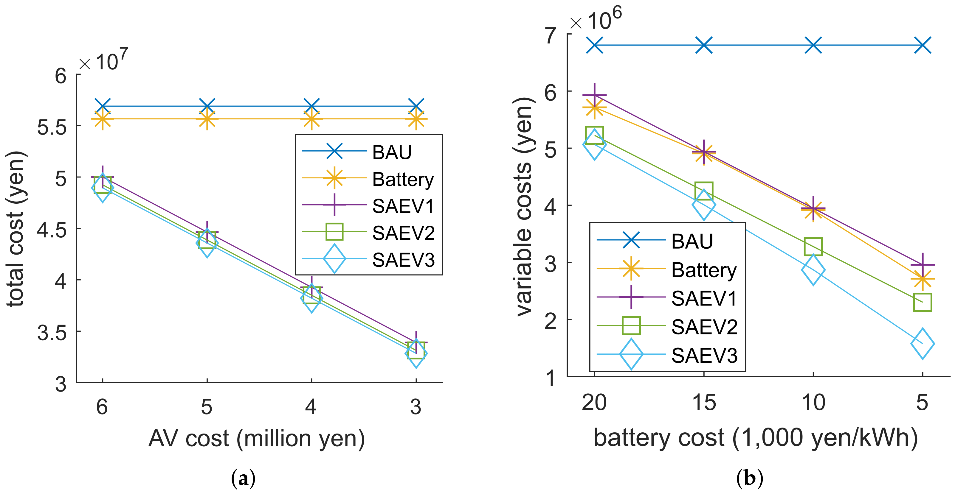
5.1.1. Sensitivity to Autonomous Driving Technology Costs

Autonomous driving technology costs are the most important factor determining the total cost of the system. This is because capital costs dominate the total costs, being about 10 times the variable costs (Table 6). However, even for the case in which vehicles cost 6 million yen ($60,000), the SAEV + VPP systems are cheaper than the alternative (Figure 5a).

5.1.2. Sensitivity to Battery Costs

The sensitivity to battery costs is presented in Figure 5b. Battery costs are a major factor in determining the operating or variable costs. Costs for SAEV with V2G decrease faster than other cases, as the lower cost of battery cycling allows vehicles to be used for grid storage. It should be noted that battery prices are expected to fall significantly in coming years. Bloomberg New Energy Finance 2017 Lithium-Ion Battery Price Survey gives average pack prices of $209/kWh (20,900 yen/kWh) in 2017, and they expect these will fall below $100/kWh (10,000 yen/kWh) by 2025 [50].

5.1.3. Sensitivity to Fuel Prices and Fuel Efficiency

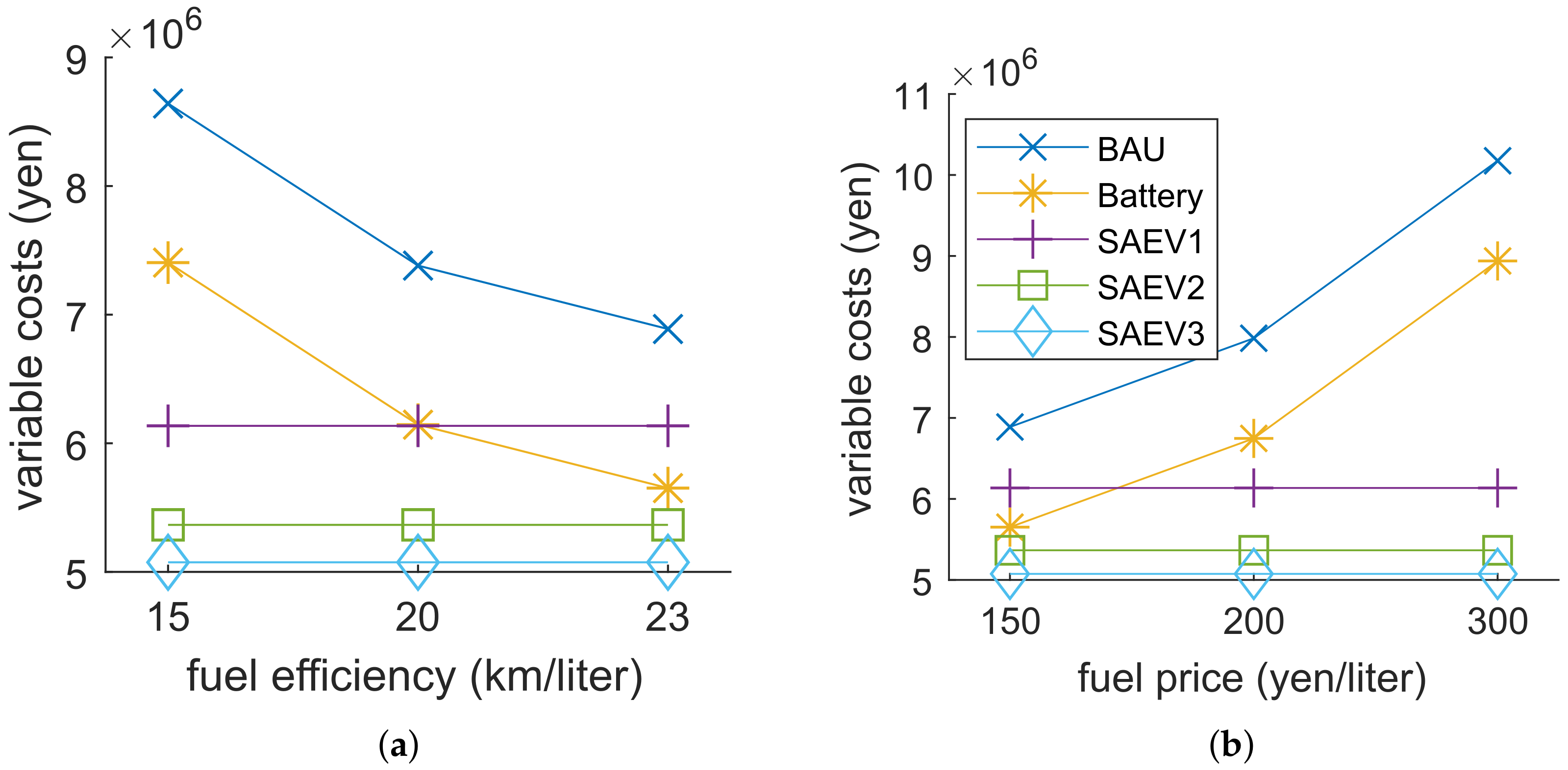
Operating or variable costs (fuel, electricity and battery) are very sensitive to fuel prices and HEV fuel efficiency. While variable costs for the BAU and battery cases are similar with SAEV cases in the baseline scenario, these costs diverge significantly with less optimistic assumptions for HEV. This is shown in Figure 6. A fuel efficiency of 20 km/liter is the target for new vehicles sold in Japan in 2020 [51]. Note that 15, 20 and 23 km/liter are equivalent to 35, 47 and 54 mpg, respectively. This is still very optimistic for HEV, and the average fuel efficiency of vehicles may be towards the lower end of the range, thus favoring SAEVs. Fuel prices may also increase as oil prices increase.

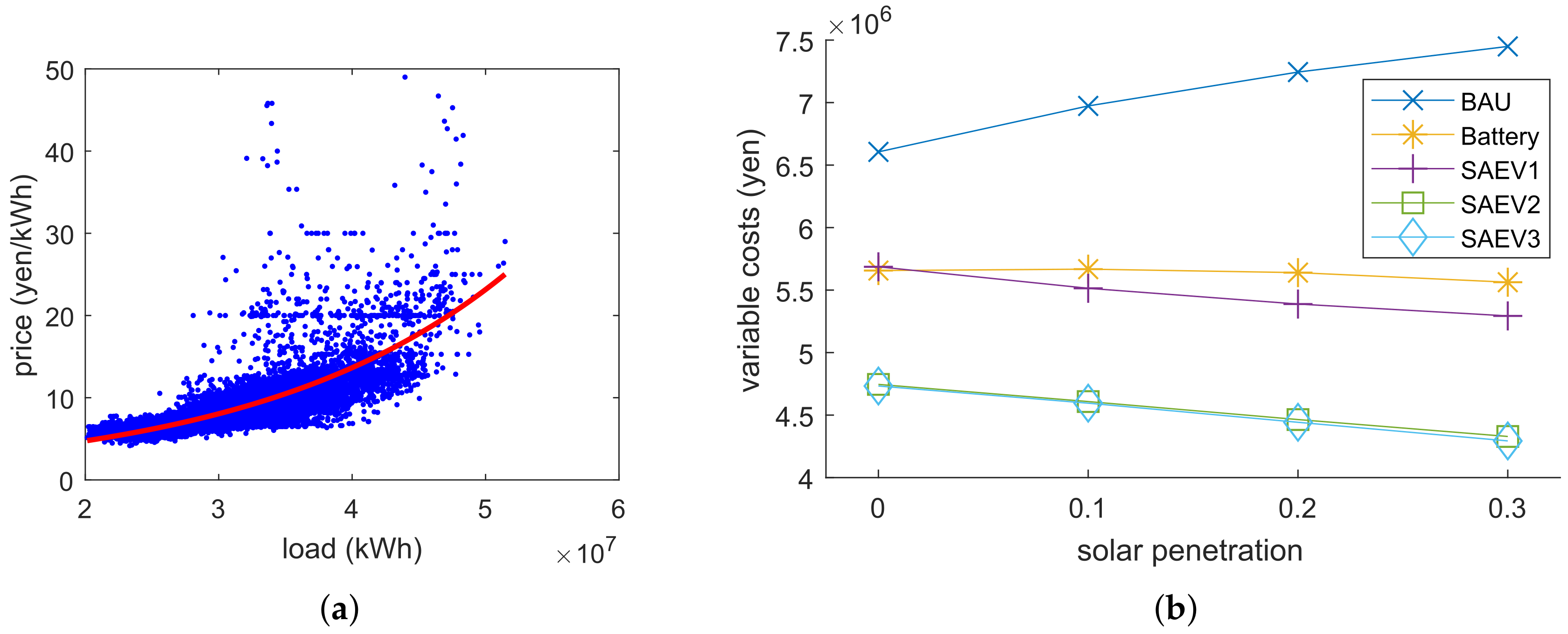
5.1.4. Effect of Increasing Solar Grid Penetration

The value of grid storage is higher with higher grid penetration of intermittent renewable energy. To test the effect of different levels of intermittent renewable energy penetration on the grid, the approximate aggregate cost curve of dispatchable generation in the TEPCO area was estimated by fitting an exponential curve to the demand/price data from JEPX (Figure 7a). This allows the generation of artificial electricity price profiles depending on load and renewable energy generation profiles. We tested the case of increasing penetration of solar power in the grid, with the results reported in Figure 7b. Higher solar penetration depresses prices paid for excess solar generation and encourages self-consumption and storage. This especially favours SAEV cases that can charge when prices are lower. The V2G case shows almost no difference with the scheduled case without V2G. This is because this simple analysis neglects some side-effects of higher solar penetration, such as the fast and expensive ramping needed at evenings. This would further increase the value of V2G providing peak generation.

5.2. Microgrid Case

The same transport, load and weather data used for the VPP were used to test the microgrid case. We assumed an isolated microgrid with no grid connection ($i_{max}=0$). We tested the same scenarios presented in Table 5 with renewable capacity sized to cover all electrical loads over a year with a 50/50% share of wind and solar power. The results are listed in

Table 7. Costs and emissions for microgrid scenarios. Fuel includes cost of fuel for cars and cost of dispatchable generators.

Scenario	Costs (Million Yen)				RE (MW)		CO${}_2$ (t)
	Fuel	Batt.	Capital	Total	Solar	Wind
BAU	8.14	0.00	48.10	56.24	12.15	7.52	181.3
Battery	5.09	3.56	48.10	56.75	12.15	7.52	117.9
SAEV1	6.64	3.96	40.11	50.71	16.55	10.24	184.5
SAEV2	4.61	3.87	40.11	48.59	16.55	10.24	131.0
SAEV3	2.62	4.46	40.11	47.19	16.55	10.24	92.7

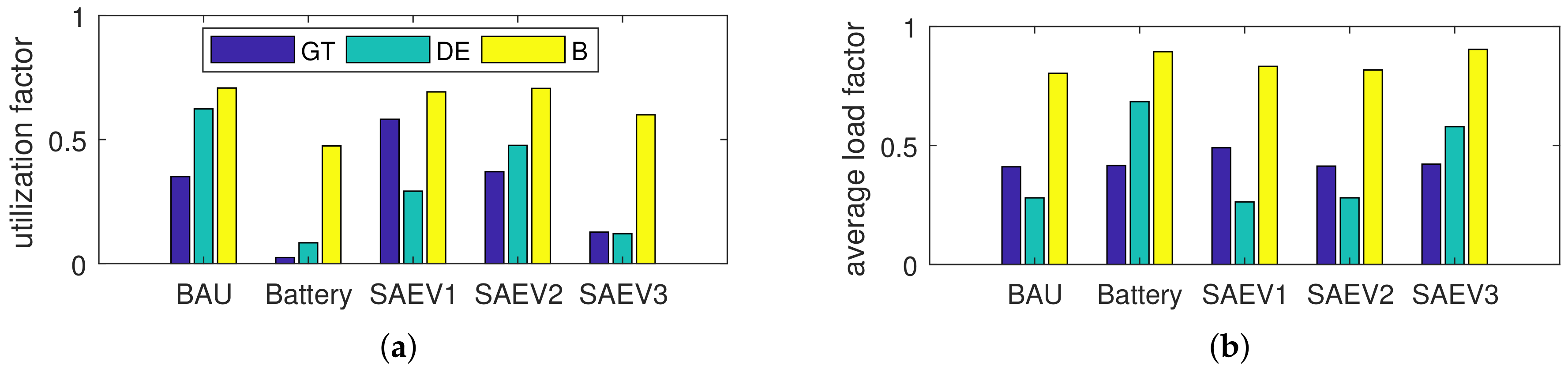
. Total costs are shown in Figure 8. An example of the results for one week with and without V2G is presented in Figure 9. In Figure 10, we report the average utilization and load factors. These are defined, respectively, as the share of time a generator is active over the whole period, and the load level of the generator when active. As generators are less efficient at lower load factors, higher load factors are preferable. The effect of lower load factor on varying the per unit carbon emissions or costs were not considered for simplicity. The cases with batteries and with SAEV + V2G show the highest load factors and the lowest utilization factors. In particular, this implies the possibility to re-size the system with less generators, thus reducing the capital costs. This effect was not considered in this work (the generators are assumed to be already present).

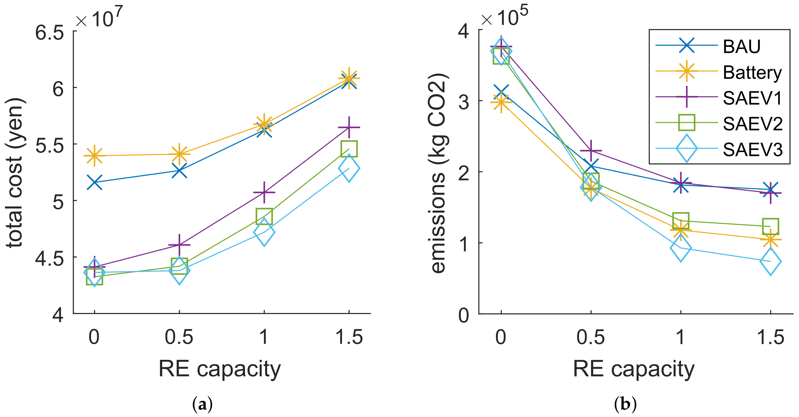
Sensitivity to Renewable Energy Capacity

The sensitivity to renewable energy capacity is shown in Figure 11. The values of capacity represent the share of yearly load generated by renewable energy. These correspond to RE capacities listed in Table 7. SAEVs are effective at integrating renewable energy in the system. The total cost for the BAU case with no renewable energy is approximately the same as for the case with SAEV + V2G with 150% renewable energy. As shown in Figure 11b, this allows a drastic decrease in carbon emissions at the same cost level.

5.3. Implications for Policy and Practice

The results suggest that there would be significant advantages for households shifting from a private vehicle to a SAEV system in the context of a VPP or in a microgrid. This could help accelerate transport electrification, provide large amount of grid storage to integrate intermittent renewable sources, and avoid the problems connected with the introduction of a large amount of non-controlled EVs on the grid. Rapidly decreasing costs of batteries and autonomous driving technology would make the system even more favorable. However, in the current situation, the system may increase carbon emissions in the Japanese context. The introduction of carbon pricing with a real-time carbon intensity signal from the grid may not only solve this problem, but also actively decrease the total carbon emissions. It should also be noted that, even though in this work we considered a constant average carbon intensity, vehicles tend to charge at periods of excess electricity generation and low prices, which often correspond to high renewable energy generation and thus lower carbon intensity.

The results may also apply to non-autonomous car sharing systems, although the cost of manual rebalancing would likely make the system more expensive and the absence of autonomous capability less attractive to users.

6. Conclusions

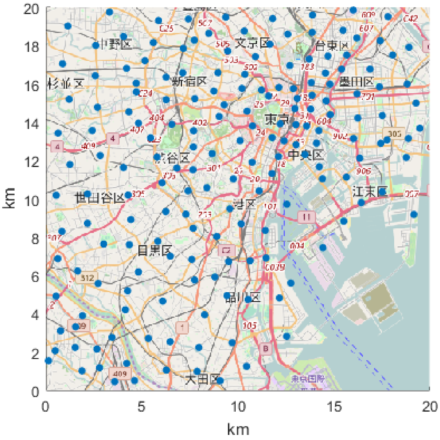
The synergies between Shared Autonomous Electric Vehicles (SAEV) and renewable energy sources were studied in the context of a grid-connected Virtual Power Plant (VPP) and an isolated microgrid. An optimization methodology was developed for the charge and discharge of the vehicles to minimize costs for the system. We tested the model with several scenarios using weather data and transport patterns for the Tokyo region. The results for the case study show that SAEV with the optimized charging are effective at decreasing the overall costs in the VPP. The proposed algorithm also decreases electricity expenditures by 75% over the unscheduled charging in the case of SAEV + V2G. Total cost savings are however dominated by capital cost savings due to lower number of vehicles needed. Overall, total costs are about 20% lower for households with rooftop solar power shifting from utility power and hybrid private vehicles to the VPP with SAEV. We also show that further electricity savings (and possibly profits) could be attained in a grid with higher penetration of intermittent renewable energy, demonstrating strong synergies existing between SAEVs and renewable energy. In the case of the isolated microgrid, SAEVs with V2G decrease cost by 16% and cut carbon emissions by half. This demonstrates the potential of SAEV to promote the integration of intermittent renewable energy while reducing total costs for the system.

This is an early work on the integration of SAEV with renewable energy, and several other aspects could be investigated in future work. Real-time grid carbon intensity could be used to extend the cost function to include carbon pricing to reduce vehicles’ emissions. In addition, an estimate of the life-cycle carbon emissions of the systems studied would allow assessing more realistically the impact of this technology. A more detailed model of dispatchable generation costs could be used to investigate more realistically the effect of increasing penetration of renewable energy in the grid and the potential for vehicles to provide grid storage. Moreover, the provision by vehicles of high revenue grid services such as frequency control or operating reserves could be included in the optimization.

References

1. Boyacı, B.; Zografos, K.G.; Geroliminis, N. An optimization framework for the development of efficient one-way car-sharing systems. Eur. J. Oper. Res. 2015, 240, 718–733. [Google Scholar] [CrossRef] [Green Version]
2. Fagnant, D.J.; Kockelman, K.M. The travel and environmental implications of shared autonomous vehicles, using agent-based model scenarios. Transp. Res. Part C Emerg. Technol. 2014, 40, 1–13. [Google Scholar] [CrossRef]
3. Weiss, J.; Hledik, R.; Lueken, R.; Lee, T.; Gorman, W. The electrification accelerator: Understanding the implications of autonomous vehicles for electric utilities. Electr. J. 2017, 30, 50–57. [Google Scholar] [CrossRef]
4. Richardson, D.B. Electric vehicles and the electric grid: A review of modeling approaches, Impacts, and renewable energy integration. Renew. Sustain. Energy Rev. 2013, 19, 247–254. [Google Scholar] [CrossRef]
5. Andersen, P.H.; Mathews, J.A.; Rask, M. Integrating private transport into renewable energy policy: The strategy of creating intelligent recharging grids for electric vehicles. Energy Policy 2009, 37, 2481–2486. [Google Scholar] [CrossRef]
6. Liu, L.; Kong, F.; Liu, X.; Peng, Y.; Wang, Q. A review on electric vehicles interacting with renewable energy in smart grid. Renew. Sustain. Energy Rev. 2015, 51, 648–661. [Google Scholar] [CrossRef]
7. Tomić, J.; Kempton, W. Using fleets of electric-drive vehicles for grid support. J. Power Sources 2007, 168, 459–468. [Google Scholar] [CrossRef]
8. Garcés Quílez, M.; Abdel-Monem, M.; El Baghdadi, M.; Yang, Y.; Van Mierlo, J.; Hegazy, O. Modelling, Analysis and Performance Evaluation of Power Conversion Unit in G2V/V2G Application—A Review. Energies 2018, 11, 1082. [Google Scholar] [CrossRef]
9. Guo, Y.; Liu, W.; Wen, F.; Salam, A.; Mao, J.; Li, L. Bidding Strategy for Aggregators of Electric Vehicles in Day-Ahead Electricity Markets. Energies 2017, 10, 144. [Google Scholar] [CrossRef]
10. Liang, H.; Zhuang, W. Stochastic Modeling and Optimization in a Microgrid: A Survey. Energies 2014, 7, 2027–2050. [Google Scholar] [CrossRef]
11. Nosratabadi, S.M.; Hooshmand, R.A.; Gholipour, E. A comprehensive review on microgrid and virtual power plant concepts employed for distributed energy resources scheduling in power systems. Renew. Sustain. Energy Rev. 2017, 67, 341–363. [Google Scholar] [CrossRef]
12. Mwasilu, F.; Justo, J.J.; Kim, E.K.; Do, T.D.; Jung, J.W. Electric vehicles and smart grid interaction: A review on vehicle to grid and renewable energy sources integration. Renew. Sustain. Energy Rev. 2014, 34, 501–516. [Google Scholar] [CrossRef]
13. Wang, J.; Liu, C.; Ton, D.; Zhou, Y.; Kim, J.; Vyas, A. Impact of plug-in hybrid electric vehicles on power systems with demand response and wind power. Energy Policy 2011, 39, 4016–4021. [Google Scholar] [CrossRef]
14. Su, W.; Wang, J.; Roh, J. Stochastic Energy Scheduling in Microgrids with Intermittent Renewable Energy Resources. IEEE Trans. Smart Grid 2014, 5, 1876–1883. [Google Scholar] [CrossRef]
15. Saber, A.Y.; Venayagamoorthy, G.K. Plug-in Vehicles and Renewable Energy Sources for Cost and Emission Reductions. IEEE Trans. Ind. Electron. 2011, 58, 1229–1238. [Google Scholar] [CrossRef]
16. Schuller, A.; Flath, C.M.; Gottwalt, S. Quantifying load flexibility of electric vehicles for renewable energy integration. Appl. Energy 2015, 151, 335–344. [Google Scholar] [CrossRef]
17. Arslan, O.; Karasan, O.E. Cost and emission impacts of virtual power plant formation in plug-in hybrid electric vehicle penetrated networks. Energy 2013, 60, 116–124. [Google Scholar] [CrossRef] [Green Version]
18. Cao, Y.; Tang, S.; Li, C.; Zhang, P.; Tan, Y.; Zhang, Z.; Li, J. An Optimized EV Charging Model Considering TOU Price and SOC Curve. IEEE Trans. Smart Grid 2012, 3, 388–393. [Google Scholar] [CrossRef] [Green Version]
19. Alonso, M.; Amaris, H.; Germain, J.; Galan, J. Optimal Charging Scheduling of Electric Vehicles in Smart Grids by Heuristic Algorithms. Energies 2014, 7, 2449–2475. [Google Scholar] [CrossRef] [Green Version]
20. Liu, H.; Ji, Y.; Zhuang, H.; Wu, H. Multi-Objective Dynamic Economic Dispatch of Microgrid Systems Including Vehicle-to-Grid. Energies 2015, 8, 4476–4495. [Google Scholar] [CrossRef] [Green Version]
21. Jin, C.; Tang, J.; Ghosh, P. Optimizing Electric Vehicle Charging With Energy Storage in the Electricity Market. IEEE Trans. Smart Grid 2013, 4, 311–320. [Google Scholar] [CrossRef]
22. Kahlen, M.; Ketter, W. Aggregating Electric Cars to Sustainable Virtual Power Plants: The Value of Flexibility in Future Electricity Markets; AAAI (Association for the Advancement of Artificial Intelligence): Menlo, CA, USA, 2015; pp. 665–671. [Google Scholar]
23. Biondi, E.; Boldrini, C.; Bruno, R. The Impact of Regulated Electric Fleets on the Power Grid: The Car Sharing Case. In Proceedings of the 2016 IEEE 2nd International Forum on Research and Technologies for Society and Industry Leveraging a Better Tomorrow (RTSI), Bologna, Italy, 7–9 September 2016; pp. 1–6. [Google Scholar] [CrossRef]
24. Zhang, R.; Rossi, F.; Pavone, M. Model Predictive Control of Autonomous Mobility-on-Demand Systems. In Proceedings of the 2016 IEEE International Conference on Robotics and Automation (ICRA), Stockholm, Sweden, 16–20 May 2016; pp. 1382–1389. [Google Scholar] [CrossRef]
25. Chen, T.D.; Kockelman, K.M.; Hanna, J.P. Operations of a shared, autonomous, electric vehicle fleet: Implications of vehicle & charging infrastructure decisions. Transp. Res. Part A Policy Pract. 2016, 94, 243–254. [Google Scholar] [CrossRef] [Green Version]
26. Bauer, G.S.; Greenblatt, J.B.; Gerke, B.F. Cost, Energy, and Environmental Impact of Automated Electric Taxi Fleets in Manhattan. Environ. Sci. Technol. 2018, 52, 4920–4928. [Google Scholar] [CrossRef] [PubMed]
27. Chen, T.; Zhang, B.; Pourbabak, H.; Kavousi-Fard, A.; Su, W. Optimal Routing and Charging of an Electric Vehicle Fleet for High-Efficiency Dynamic Transit Systems. IEEE Trans. Smart Grid 2018, 9, 3563–3572. [Google Scholar] [CrossRef]
28. Spieser, K.; Treleaven, K.; Zhang, R.; Frazzoli, E.; Morton, D.; Pavone, M. Toward a Systematic Approach to the Design and Evaluation of Automated Mobility-on-Demand Systems: A Case Study in Singapore. In Road Vehicle Automation; Meyer, G., Beiker, S., Eds.; Springer International Publishing: Cham, Switzerland, 2014; pp. 229–245. [Google Scholar] [Green Version]
29. Rubner, Y. Code for the Earth Movers Distance (EMD). Available online: http://ai.stanford.edu/ rubner/emd/default.htm (accessed on 2 November 2017).
30. Tushar, M.H.K.; Assi, C.; Maier, M.; Uddin, M.F. Smart Microgrids: Optimal Joint Scheduling for Electric Vehicles and Home Appliances. IEEE Trans. Smart Grid 2014, 5, 239–250. [Google Scholar] [CrossRef]
31. HOMER. HOMER® Pro Version 3.7 User Manual; HOMER Energy LLC: Boulder, CO, USA, August 2016. [Google Scholar]
32. Ministry of Land, Infrastructure, Transport and Tourism, Japan (MLIT). Tokyo Metropolitan Area Person Trip Survey; MLIT: Tokyo, Japan, 2008.
33. Iacobucci, R.; McLellan, B.; Tezuka, T. Modeling shared autonomous electric vehicles: Potential for transport and power grid integration. Energy 2018. [Google Scholar] [CrossRef]
34. Tokyo Electric Power Company Holdings, Inc. (TEPCO). Electricity Forecast|Download past Electricity Demand Data; TEPCO: Tokyo, Japan, 2018; Available online: http://www.tepco.co.jp/en/forecast/html/download-e.html (accessed on 2 February 2018).
35. Statistics Bureau, Ministry of Internal Affairs and Communications. Japan Statistical Yearbook—Chapter 11 Energy and Water; Statistics Bureau, Ministry of Internal Affairs and Communications: Tokyo, Japan, 2018.
36. Japan Meteorological Agency. Data of Solar and Infrared Radiation; Japan Meteorological Agency: Tokyo, Japan, 2018. Available online: https://www.data.jma.go.jp/gmd/env/radiation/en/info_rad_e.html (accessed on 1 August 2018).
37. NOAA. Climate Data Online. Available online: https://www7.ncdc.noaa.gov/CDO/cdo (accessed on 26 November 2017).
38. International Renewable Energy Agency (IRENA). Renewable Power Generation Costs in 2017; IRENA: Abu Dhabi, UAE, 2017. [Google Scholar]
39. Intergovernmental Panel on Climate Change. Climate Change 2014 Mitigation of Climate Change: Working Group III Contribution to the Fifth Assessment Report of the Intergovernmental Panel on Climate Change; Cambridge University Press: Cambridge, UK, 2014. [Google Scholar] [CrossRef]
40. Nykvist, B.; Nilsson, M. Rapidly falling costs of battery packs for electric vehicles. Nat. Clim. Chang. 2015, 5, 329–332. [Google Scholar] [CrossRef] [Green Version]
41. Hao, H.; Mu, Z.; Jiang, S.; Liu, Z.; Zhao, F. GHG Emissions from the Production of Lithium-Ion Batteries for Electric Vehicles in China. Sustainability 2017, 9, 504. [Google Scholar] [CrossRef]
42. U.S. Department of Energy (DOE). Compare Side-by-Side 2016 Toyota Prius; DOE: Washington, DC, USA, 2016.
43. JAMA. The Motor Industry of Japan 2017; JAMA: Tokyo, Japan, 2017. [Google Scholar]
44. Fagnant, D.J.; Kockelman, K. Preparing a nation for autonomous vehicles: opportunities, barriers and policy recommendations. Transp. Res. Part A Policy Pract. 2015, 77, 167–181. [Google Scholar] [CrossRef]
45. IHS Automotive. Emerging Technologies: Autonomous Cars— Not If, But When; IHS Automotive: Southfield, MI, USA, 2014. [Google Scholar]
46. The Federation of Electric Power Companies of Japan (FEPC). Electricity Review Japan; FEPC: Tokyo, Japan, 2017. [Google Scholar]
47. Ministry of Economy, Trade and Industry (METI). Available online: http://www.meti.go.jp/english/ (accessed on 1 August 2018).
48. Iwafune, Y.; Ikegami, T.; Fonseca, J.G.d.S.; Oozeki, T.; Ogimoto, K. Cooperative home energy management using batteries for a photovoltaic system considering the diversity of households. Energy Convers. Manag. 2015, 96, 322–329. [Google Scholar] [CrossRef]
49. Adefarati, T.; Papy, N.B.; Thopil, M.; Tazvinga, H. Non-renewable Distributed Generation Technologies: A Review. In Handbook of Distributed Generation; Springer: Cham, Switzerland, 2017; pp. 69–105. [Google Scholar]
50. Chediak, M. The Latest Bull Case for Electric Cars: the Cheapest Batteries Ever. 2017. Available online: Bloomberg.com (accessed on 28 June 2018).
51. Japan Automobile Manufacturers Association. The Motor Industry of Japan; Japan Automobile Manufacturers Association (JAMA): Tokyo, Japan, 2015. [Google Scholar]
Figure 1. Model flow diagram.
Energies 11 02016 g001
Figure 2. Transport demand and renewable energy generation. (a) EMD for trips from the transport survey during a day; and (b) Example of profiles for solar and wind power generation during a week.
Energies 11 02016 g002
Figure 3. Map of origin/destination nodes in central Tokyo, taken from transport survey [32]. Map from Openstreetmap
Energies 11 02016 g003
Figure 4. Weekly total costs for 100 iterations for each case considered.
Energies 11 02016 g004
Figure 5. Sensitivity of: (a) Total costs to autonomous vehicle cost; and (b) Variable costs (electricity, fuel, and battery costs) to battery costs.
Energies 11 02016 g005
Figure 6. Sensitivity of variable costs to: (a) HEV fuel efficiency; and (b) Fuel cost.
Energies 11 02016 g006
Figure 7. Effect of increasing solar penetration in the grid (a) Exponential fit of the relation between prices and dispatchable generation on the Japan Electric Power Exchange (JEPX) in 2017; and (b) Variable costs of the system for increasing solar penetration.
Energies 11 02016 g007
Figure 8. Weekly average total costs for the cases considered in the microgrid case.
Energies 11 02016 g008
Figure 9. Example of SOC, charge (C), load (L) and generation from gas (GT), diesel (DE), biomass (B), solar (S) and wind (W): (a) Without V2G; and (b) With V2G. V2G discharge (negative charge) allows avoiding gas turbine and diesel generator start-up.
Energies 11 02016 g009
Figure 10. Microgrid distributed generators use: (a) utilization factor and (b) load factor for gas turbine (GT), diesel engine (DE), and biomass (B) in the microgrid case.
Energies 11 02016 g010
Figure 11. Microgrid case. Sensitivity to total renewable energy (RE) capacity of: (a) total costs; and (b) carbon emissions.
Energies 11 02016 g011