Stability Analysis of Grid-Connected Converters with Different Implementations of Adaptive PR Controllers under Weak Grid Conditions


State Key Laboratory of Advanced Electromagnetic Engineering and Technology, School of Electrical and Electronic Engineering, Huazhong University of Science and Technology, Wuhan 430074, China
*
Author to whom correspondence should be addressed.
Energies 2018, 11(8), 2004; https://doi.org/10.3390/en11082004
Submission received: 10 July 2018
/
Revised: 30 July 2018
/
Accepted: 31 July 2018
/
Published: 1 August 2018
(This article belongs to the Special Issue Power Electronics in Renewable Energy Systems)
Abstract
:Adaptive proportional resonant (PR) controllers, whose resonant frequencies are obtained by the phase-locked loop (PLL), are employed in grid connected voltage source converters (VSCs) to improve the control performance in the case of grid frequency variations. The resonant frequencies can be estimated by either synchronous reference frame PLL (SRF-PLL) or dual second order generalized integrator frequency locked loop (DSOGI-FLL), and there are three different implementations of the PR controllers based on two integrators. Hence, in this paper, system stabilities of the VSC with different implementations of PR controllers and different PLLs under weak grid conditions are analyzed and compared by applying the impedance-based method. First, the αβ-domain admittance matrixes of the VSC are derived using the harmonic linearization method. Then, the admittance matrixes are compared with each other, and the influences of their differences on system stability are revealed. It is demonstrated that if DSOGI-FLL is used, stabilities of the VSC with different implementations of the PR controllers are similar. Moreover, the VSC using a DSOGI-FLL is more stable than that using a SRF-PLL. The simulation and experimental results are conducted to verify the correctness of theoretical analysis.
1. Introduction
With the increasing energy consumption worldwide, the use of renewable energy sources like wind and solar energies [1,2] in the grid has been growing increasingly. The voltage source converters (VSCs) have many desirable features, such as full controllability, low current harmonics, and high efficiency, thus they are widely used to deliver the power produced by the renewable energies into the grid [3].
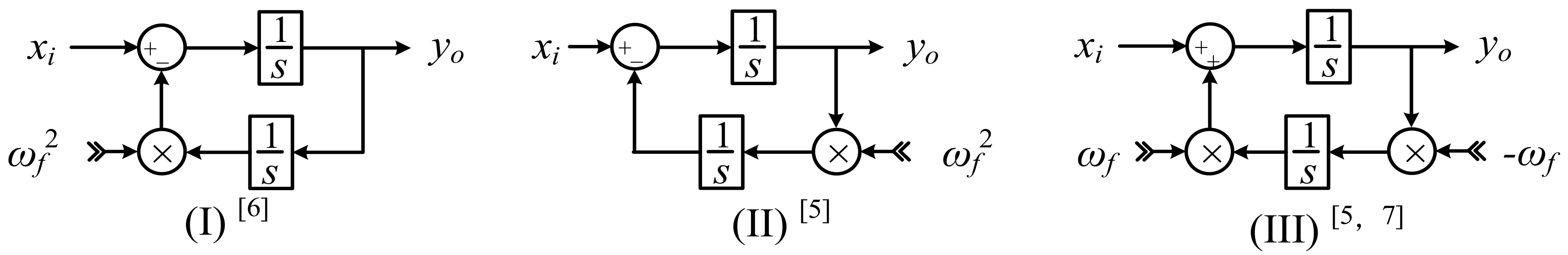
Proportional resonant (PR) controllers could control positive-sequence and corresponding negative-sequence grid current at the same time without any additional negative-sequence current controller, and they allow a relatively low computational cost as they are implemented in the stationary frame [3,4,5]. Hence, PR controllers working on the stationary reference frame are widely used in grid-connected VSCs. Implementations of the PR controllers based on two integrators are widely employed, since no explicit trigonometric functions are needed [5]. Three typical implementations of the resonance term of the current controllers in the prior studies are shown in Figure 1 [5,6,7]. For future reference, they are called implementation I, II and III, respectively. If the resonant frequency is constant, these implementations are equivalent to each other.
The grid frequency is practically not a constant but within a certain range [8,9], thus the control performance would be inevitable weakened if the center frequency of the resonance controller is set to be constant. If the resonant frequency is set to be the fundamental frequency and the grid frequency deviates from it, there would be a phase shift between the grid current and the corresponding grid voltage, though the aimed power factor is unity [6]. To improve control performance in the case of grid frequency variations, the authors of [6,8,10,11,12,13] developed frequency adaptive PR controllers, whose resonant frequencies are not constant values, but are updated online according to the frequency estimated by the phase-locked loop (PLL) system. If the adaptive PR controllers are applied, a unity power factor operation can be achieved [6]. The resonant frequency of the adaptive PR controller is time-variant, thus dynamic properties of the adaptive PR controllers with different implementations might be dramatically different. Consequently, the port characteristics of the converter with different implementations of adaptive PR controllers would not be the same.
The resonant frequency of the adaptive PR controller can be obtained by grid synchronization techniques based on phase locking approach, e.g., synchronous reference frame-phase locked loop (SRF-PLL) [14] which is widely used for its simplicity and robustness, or frequency locking approach, e.g., dual second-order generalized integrator-frequency locked loop (DSOGI-FLL) [15] which is implemented in the stationary reference frame. As SRF-PLL and DSOGI-FLL use different approaches to obtain the grid frequency, their influences on the port characteristics of the converter with adaptive current controllers might differ be different.
Under weak grid conditions, stability issues introduced by the grid-connected VSCs are of great importance [16,17,18,19,20,21,22]. The differences of the port characteristics of the converter introduced by applying different control schemes, including three different implementations of the adaptive PR controllers and the two different PLLs to obtain the resonant frequency, might significantly change the stability of the VSC connected to a weak grid. Hence, it is necessary to compare the robustness of the VSC with different control schemes.
In this paper, the stability issues of the VSC with different implementations of the adaptive PR controllers and different PLLs are studied and analyzed using the impedance-based method [18,23,24,25,26,27,28]. A suggestion to choose a suitable controllers’ implementation and the related PLL for the VSC with adaptive PR controllers is given.
The rest of the paper is organized as follows: in Section 2, the studied system with adaptive current controller is briefly introduced. Section 3 shows how to model the adaptive resonant controller with different implementations of the resonant terms, and the approach to incorporate it into the admittance model of the converter. In Section 4 the effects of the adaptive resonant controllers with different implementations on system stability is analyzed and compared, and the stability of the system using a SRF-PLL for grid synchronization and the system using a DSOGI-FLL for grid synchronization is compared. Section 5 includes experimental verifications of the theoretical analysis. Section 6 concludes this paper.
2. VSC with Adaptive PR Current Controllers
The L-type grid connected converter with grid current regulation working on αβ reference frame is studied, as depicted in Figure 2. The inductance of the filter is L, and the equivalent series resistance is r. The grid inductance is Lg. The grid voltages, the voltages at the point of common coupling (PCC), the ac-side converter voltages, and the currents delivered to the grid are usk, ugk, vk, and ik (k = a, b, c), respectively. The dc input voltage of the converter is Vdc.
Grid current references in the stationary reference frame (iαr, iβr) can be obtained by applying an inverse Park transformation to the active, reactive current references (Idr, Iqr). In this paper, unit-power factor is considered, i.e., Iqr is set to be zero. Subscripts ‘α’ and ‘β’ refer to the α-axis and β-axis, respectively, while subscripts ‘d’ and ‘q’ refer to the d-axis and q-axis, respectively.
2.1. Adaptive PR Controller
The grid current error signals (eα, eβ) are sent to the PR controllers to generate the reference of the ac-side converter voltages (vαr, vβr). The PR current controllers are defined as follows:
where ωf is the resonant frequency, different from the conventional PR controller, the adaptive PR controller uses the frequency estimated by the PLL as the resonant frequency instead of the constant fundamental frequency ω1; kp, kr are the proportional- and resonant-gain of the controller, respectively. The controller gains can be tuned according to: kp = αcL, ki = αcr [18] where αc is the current control loop bandwidth. R(s) is the resonant term of the controller. R(s) has infinite gain at the resonant frequency and thus it is capable for the grid current to track its reference without steady-state error.
The detailed block diagrams of different implementations of the PR controller based on two integrators are depicted in Figure 3, where xiα and yoα are the input and output of R(s), respectively. The α-axis and β-axis are decoupled, thus only the PR controller implemented in the α-axis is given for simplicity. In time domain, the relationships between xiα and yoα can be derived from Figure 3, as follows:
where Equations (2-I), (2-II) and (2-III) are obtained with implementation I, II, and III of the PR controllers, respectively. If ωf is constant, the three equations are equivalent to each other. However, for the adaptive PR controllers, ωf is time varying, the equations are no longer the same. Thus the dynamic properties of the adaptive PR controllers with different implementations might be different, and the transfer function shown in Equation (1) is not enough to describe the dynamic properties of adaptive PR controllers.
The adaptive PR controllers’ outputs are sent to the SVPWM to generate the control signals.
2.2. Grid Synchronization Methods
Two typical grid synchronization methods, i.e., SRF-PLL and DSOGI-FLL as shown in Figure 4 are used to provide the phase angle to calculate the reference currents and the controller’s resonant frequency. The block diagram of a typical SRF-PLL is shown in Figure 4a, where GPLL(s) is the PLL controller. Figure 4b shows the block diagram of DSOGI-FLL with frequency locked loop (FLL) gain normalization, where k is the gain of the SOGI, and γ is used to regulate the settling time of the FLL [22]. The DSOGI-FLL consists of four parts: (1) SOGI; (2) positive/negative-sequence calculation block (PNSC) to obtain the positive-sequence voltages (uα+, uβ+) and the negative-sequence voltage (uα−, uβ−); (3) FLL with FLL gain normalization to estimate the grid frequency; (4) the “atan2” uses the positive-sequence voltages for the phase angle calculation.
With different implementations of the adaptive PR controllers and different PLLs, the stability of the grid-connected converter might be quite different under weak grid conditions.
3. Impedance Modeling
Impedance-based methods were a popular choice in prior studies to analyse the stability of grid-connected converters. Impedance modeling of the converter can be performed in either the dq-domain [25] or in the αβ-domain [26,27]. Considering that the grid current regulation working on αβ reference frame is used, impedance-based method in the αβ-domain is applied in this paper. The αβ-domain converter impedances are derived using harmonic linearization method.
A positive-sequence perturbation at an arbitrary frequency ωp is injected to the grid to obtain the reflected admittances at the ac terminals. Thus, in three phase variables, there would have positive-sequence components at frequency ωp and negative-sequence components at frequency ωp − 2ω1 [28]. In this paper, it is defined that s = jω, where ω = ωp − ω1.
3.1. Model of the Adaptive PR Controllers
The outputs of the adaptive PR controllers are affected by the error signal and the estimated frequency, as shown in Figure 3, thus the small-signal part of controllers’ outputs can be described by Equation (3):
where H(s) is defined in Equation (1); (s) and (s) are used to describe the influence of ωf on the positive-, negative-sequence components of the current controllers’ outputs, respectively. The superscripts of the variables ‘p’ and ‘n’ are used to indicate the positive-, negative-sequence of the variables, respectively. The superscripts of the transfer functions ‘x’ in (s) and (s) is used to distinguish the implementations of adaptive controllers: x = i, ii, and iii indicates that implementation I, II and III is used, respectively.
To obtain the detailed expressions of (s) and (s), eα is assumed to be zero, thus from Figure 3, it can be easily obtained that xiα = 0, and yoα = vαr. If the implementation I of the adaptive PR controller is used, it can be derived from (2-I) by using convolution that:
where Vα[±ω1] = (Vm + rIdr ± jLω1Idr)/2 are the Fourier coefficients of vαr at the positive/negative fundamental frequency, Vm is the magnitude of PCC voltage. For simplicity, set Vp = 2Vα[ω1], and Vn = 2Vα[−ω1].
3.2. Model of the PLL System
The frequency domain forms of ωf and θf are shown in Equation (5). The superscripts ‘y’ is used to distinguish the PLL that is applied: y = pll means that a SRF-PLL is used; y = fll means that a DSOGI-FLL is used. The expressions of the transfer functions are shown in Table 2 where Tpll(s) = GPLL(s)/(s + VmGPLL(s)) and D(s) = s2 + kω1s + ω12. The derivations are shown in the Appendix A.
3.3. Model of the Current References
3.4. Model of the Grid Current Loop
Based on the adaptive PR controller (3), the PLL system (5) and the current references (6), the detailed small-signal model of the grid current with adaptive PR controllers can be obtained, as depicted in Figure 5, where Gd(s) is used to depicts the gain and delays (digital computation delay and the PWM delay) [29] of the converter, as follows:
where Ts is the sampling period.
Because of the adaptive PR controller, extra branches are introduced in the model of grid current loop, as shown in the red part of Figure 5. Moreover, (s), (s) (as shown in Table 1) are different for different implementations of adaptive PR controllers, and (s), (s) (as shown in Table 2) are not the same for different PLLs. Hence, the port characteristics of the grid-connected converters with different implementations of the adaptive PR controllers and different PLLs are different.
3.5. Admittance Matrix
The admittance matrix of the converter, Yαβ(s), is defined in Equation (10):
The elements can be derived from Figure 5, as follows:
4. Impedance-Based Stability Analysis
4.1. Addmittances Analysis and Verifications
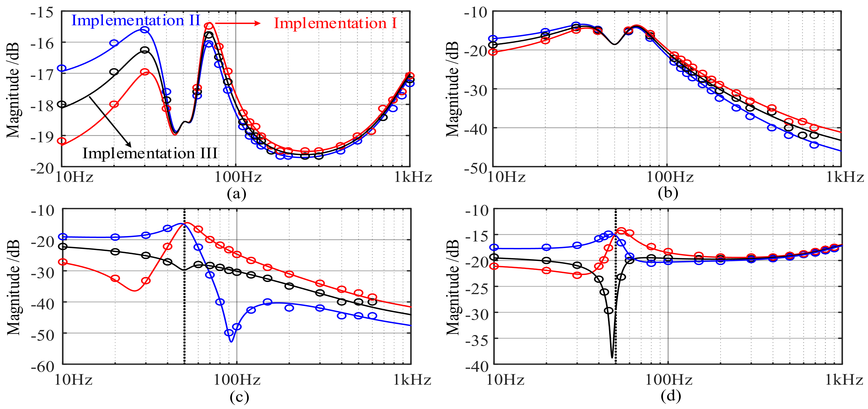
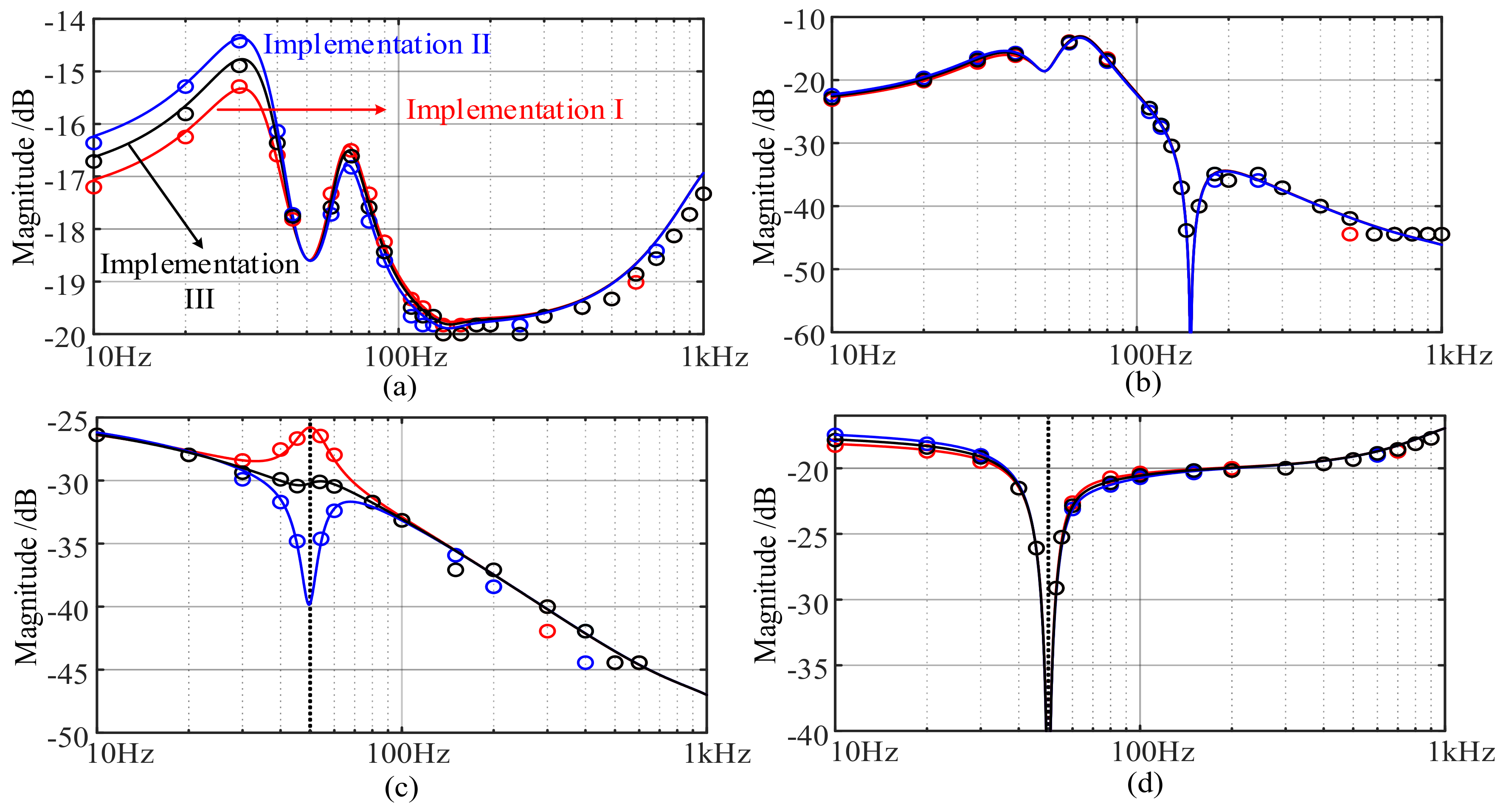
Figure 6 and Figure 7 shows the magnitude responses of the admittances of the grid-connected converter with SRF-PLL and DSOGI-FLL, respectively. The solid lines are plotted using the theoretical models in Equation (11), while the circles are the point-by-point numerical simulation results of the admittances for comparison. The parameters used in simulations are as shown in Table 3 with the bandwidth of the SRF-PLL fbω_PLL = 40 Hz (the corresponding parameters of the GPLL(s) is designed based on [30]), and the parameters of the DSOGI-FLL are: k = 1.1, γ = 41. It can be observed from Figure 6 and Figure 7 that for different implementations of adaptive PR controllers and different PLLs, the numerical admittances match the theoretical admittances of the grid-connected converter, which verify the correctness of the proposed admittance model.
4.1.1. SRF-PLL is Used for Grid Synchronization
It can be observed from Figure 6 that the Ypp(s + jω1) and Ypn(s + jω1) with different implementations of the adaptive controllers are similar as shown in Figure 6a,b, while Ynp(s − jω1) and Ynn(s − jω1) are different, especially at the frequencies around s − jω1 = jω1, i.e., s = j2ω1, as shown in Figure 6c,d. The value of Ynp(s − jω1) and Ynn(s − jω1) at s = j2ω1 can be obtained by Equation (11), as follows:
where Equations (12-I), (12-II), and (12-III) are the admittances of the converter with implementation I, II, and III of the adaptive PR controller, respectively.
Obviously, it can be obtained from Equation (12) that for a small kr as suggested in [16], the magnitudes of Ynp(s − jω1) and Ynn(s − jω1) of the converter using implementation III around s = j2ω1 are much smaller than those using implementation I or II.
4.1.2. DSOGI-FLL is Used for Grid Synchronization
It can be observed from Figure 7 that for different implementations of the adaptive resonant controllers, the converter admittances Ypp(s + jω1), Ypn(s + jω1), Ynn(s − jω1) are similar, while Ynp(s − jω1) are different at the frequencies around s = j2ω1. Due to the effect of the zeros in (s − jω1) and (s − jω1) (as shown in Table 2) at s = j2ω1, it can be derived from Equation (11) that:
Equation (13) is valid with different implantations of the adaptive PR controllers.
4.2. Stability Analysis
4.2.1. Stability Criterion
System stability is determined by applying general Nyquist stability criterion to the minor loop gain Lαβ(s) = Zgαβ(s)Yαβ(s), where Zgαβ(s) is the impedance matrix of the grid as shown in Equation (14) [28]. The system is stable if the Nyquist curves of the eigenvalues of Lαβ(s), i.e., λ1(s) and λ2(s) as defined in Equation (15), do not encircle the critical point (−1, j0), otherwise, the system is unstable [27,28]:
4.2.2. Stability Analysis with Different PLLs
Figure 8 shows the Nyquist curves of characteristic loci of the grid system using different implementations of the adaptive current controllers and different PLLs. The parameters used in simulations are as shown in Table 3 with fbω_PLL = 75 Hz, the parameters of the DSOGI-FLL are: k = 1.1, γ = 41, and the grid inductance Lg = 6 mH.
It can be observed from Figure 8a that if a DSOGI-FLL is used, the stabilities of grid-connected converters with different implementations of the adaptive PR controllers are similar. Since Ypn(j3ω1) = 0 as derived in Equation (13), Ypn(s + jω1) × Ynp(s − jω1) are very small around s = j2ω1. Therefore, based on Equation (15), it can be concluded that although that Ynp(s − jω1) are different around s = j2ω1, the differences would have very limited influence on the λ1(s) and λ2(s).
It can be observed from Figure 8b that if a SRF-PLL is used, the stabilities of grid-connected converters with different implementations of the adaptive PR controllers are quite different. The converter with implementation I is unstable, while the converter with implementation II and III are stable. The stability boundaries of the grid-connected converters with different implementations of the adaptive PR controllers are obtained based on the stability criterion, as depicted in Figure 9. It can be observed from Figure 9 that the system with implementation III has the largest stable region, while the system with implementation I has the smallest stable region. When the short circuit ratio (SCR) is set to be 2.23, the maximum bandwidth to maintain system stability is around 73.3 Hz if implementation I is used, the maximum value extends to about 107.9 Hz if implementation II is applied, and the maximum value can be further raised to about 121.2 Hz if implementation III is applied. Above all, implementation III of the adaptive PR current controllers is suggested to be used for the grid connected converter using SRF-PLL for grid synchronization.
4.2.3. Comparison with Different PLLs
In this subsection, the effects of the SRF-PLL and DSOGI-FLL on stability of the grid connected converter with adaptive resonance current controllers using implementation III are compared.
Based on Equation (6), the dynamic properties of the output angle of a SRF-PLL with fbω_PLL = 40 Hz and a DSOGI-FLL with k = 1.1, γ = 41 are similar, as shown in Figure 10a. Under this circumstance, Figure 10b shows the corresponding dynamic properties of the output frequency for different PLLs. The magnitudes of (s) and (s) are smaller than that of (s) and (s), hence it can be concluded that ωf is more robust if the DSOGI-FLL is used than that if the SRF-PLL is used. The influence of a PLL on system stability depends on the dynamic properties of the output phase angle and the estimated frequency. Hence, the converter using DSOGI-FLL for grid synchronization should be more stable than the converter using SRF-PLL for grid synchronization.
Figure 11 shows the corresponding Nyquist curves of characteristic loci of converters with different synchronization method. The other parameters used in the simulation are as shown in Table 3. It can be concluded from Figure 11 that the converter using DSOGI-FLL for grid synchronization has a larger stability margin than that of the converter using SRF-PLL.
5. Experimental Verifications
A three-phase grid-connected converter has been built and tested to verify proposed analysis. The current controllers, frame transformation and the PLL were implemented in a TMS320F28335 DSP board (Texas Instruments, Inc, Dallas, TX, USA). The grid current is sensed by a TCP0150 current probe (Tektronix, Beaverton, OR, USA) and the bandwidth of the SRF-PLL fbw_PLL, the q-axis component of the grid current iq, and the estimated frequency ωf are sent to the D/A in the board as output signals. The output of the D/A cannot be negative, hence, it is programed to have a 15 A offset in iq and a 200 rad/s offset in ωf compared to the corresponding actual values. Parameters for this experimental setup are provided in Table 3, which are consistent with the simulation parameters. The parameters of DSOGI-FLL are: k = 1.1, γ = 41, and the short circuit ratio is 2.23 (the corresponding Lg is 6 mH).
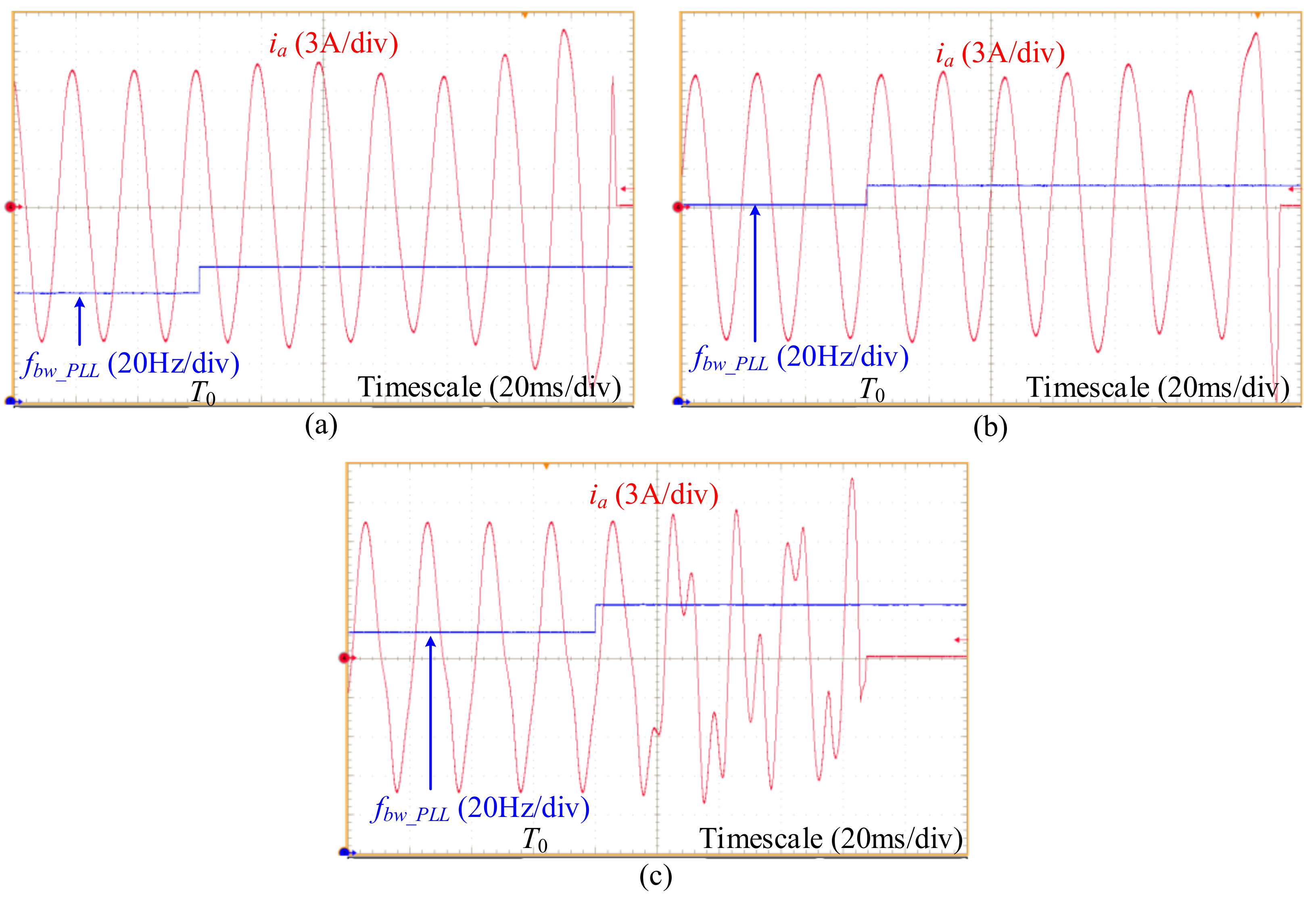
Figure 12 are the experimental waveforms of A-phase current of the converter using SRF-PLL for grid synchronization. In Figure 12a, the implementation I of the adaptive resonance controller is applied. At time T0, the bandwidth of the PLL jumps from 56 Hz to 70 Hz, and after T0, the grid current diverges. Once the grid currents reach the up-limited value, the system would stop running. In Figure 12b, the implementation II is applied. At time T0, the bandwidth of the PLL jumps from 102 Hz to 112 Hz, and after T0, system becomes unstable. In Figure 12c, the implementation III is applied. At time T0, the bandwidth of the PLL jumps from 114 Hz to 126 Hz, and after T0, system is no longer stable. The experimental results match the theoretical stability boundaries shown in Figure 9.
Figure 13 shows the experimental waveforms of ia, ωf, and iq of the grid connected converter using DSOGI-FLL for grid synchronization. In Figure 13a–c, implementation I, II and III of the adaptive PR controllers are used, respectively. The active current reference Idr changes from 0 A to 10 A at time T0, and the dynamic responses of ωf, and iq are similar for all implementations of the adaptive PR controllers. The experimental results match the theoretical analysis in Section 4.2.2.
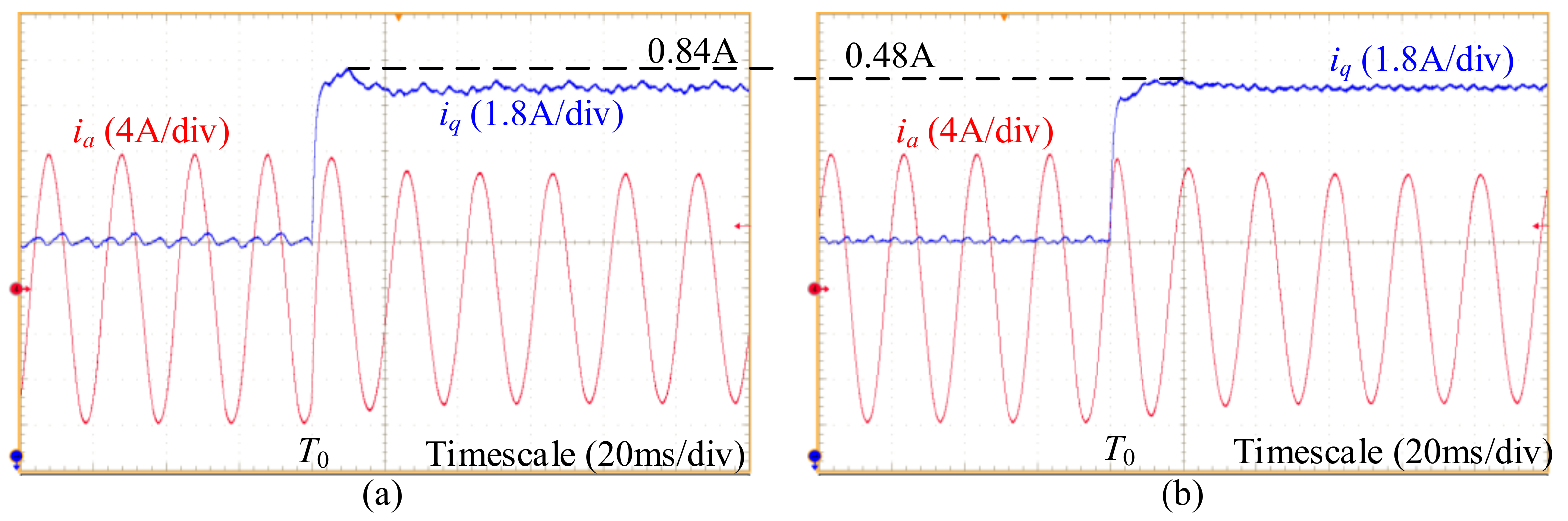
Figure 14 shows the experimental waveforms of A-phase current and iq of the grid connected converter with Implementation III of the adaptive PR controllers. In Figure 14a, the SRF-PLL with 40 Hz bandwidth is applied while in Figure 14b, the DSOGI-FLL is used. The reactive current reference Iqr changes from −6 A to 0 A at time T0. It is can be obtained from Figure 14 that: the percentage overshoot (PO) of iq in Figure 14a is about 14% (0.84/6) while in Figure 14b the PO is less than 8% (0.48/6). The system with DSOGI-FLL has a stronger damping than that of the system with SRF-PLL. The experimental results verify the effectiveness of the analysis in Section 4.2.3.
6. Conclusions
The impedance model and stability of the grid-connected VSCs with adaptive resonance current controllers has been explored in this paper. Based on the proposed small-signal impedance model, some tips should be aware of when implementing adaptive resonant controllers:
- (1)
- If a SRF-PLL is used for grid synchronization, the system using implementation III of the resonant controller has the best stability margin, while the system using implementation I has the worst stability margin under weak grid conditions.
- (2)
- If a DSOGI-FLL is used for grid synchronization, the systems using implementation I, II, and III of the resonant controller have similar stability margins.
- (3)
- The system using a DSOGI-FLL for grid synchronization has a larger stability margin than that of the system using a SRF-PLL if the dynamic property of the output angle of the two synchronization methods are similar.
Experimental results validate the conclusions based on the theoretical analysis. In sum, the implementation of the resonance controller and the grid synchronization method should be carefully chosen for the weak-grid connected converter using adaptive resonance current controllers.
Author Contributions
X.L. proposed the main idea, performed the theoretical analysis, performed the experiments, and wrote the paper; H.L. contributed the experiment materials, and gave some suggestions to the paper writing.
Funding
This research received no external funding.
Conflicts of Interest
The authors declare no conflict of interest.
Appendix A
Appendix A.1. Modeling of the SRF-PLL
It can be obtained from [22] that, the output angle of the SRF-PLL is:
where Tpll(s) is the close loop gain of the PLL, as follows:
The estimated frequency is in fact the differential of the output angle of the PLL, i.e., ωf(ω) = sθf(ω), hence, from Equation (A1) it can be obtained that:
Appendix A.2. Modeling of the DSOGI-FLL
Appendix A.2.1. Modeling of the SOGIs
According to the block diagram shown in Figure 4b, it can be obtained that:
The steady-state value of the uα is Vmcos(ω1t), by using convolution, it can be obtained that:
With Equations (A4)–(A6), it can be obtained that:
where D(s) = s2 + kω1s + ω12 is used to simplify the expression.
Appendix A.2.2. Modeling of the PNSC
For a balanced positive-, negative-sequence vector, the α-, β-axis components keep the following steady-state relationship on frequency domain:
Thus, the input signals of the “atan2” are:
Appendix A.2.3. Modeling of the FLL
The steady state values of εα, εβ are zeros, while quα, quβ are Vmsin(ω1t) and −Vmcos(ω1t), respectively. Hence, by using convolution, it can easily be obtained that:
Using the similar steady-state relationship as shown in Equation (A10), Equation (A12) can be simplified as follows:
The steady-state value of uf is zero, hence the output of the FLL can be written as follows:
With Equations (A9), (A13), and (A14), the output of the FLL can be obtained that:
Appendix A.2.4. Modeling of the Output Angle
As demonstrated in [31], the output angle of “atan2” satisfies the following relationship:
It is pointed out in [27,28] that the vector at frequency ω − ω1 is not positive-sequence, but negative-sequence, hence, Equation (A16) can be simplified to:
With Equations (A11), (A15), and (A17), it can be obtained that:
References
- Blaabjerg, F.; Chen, Z.; Kjaer, S.B. Power electronics as efficient interface in dispersed power generation systems. IEEE Trans. Power Electron. 2004, 19, 1184–1194. [Google Scholar] [CrossRef]
- Dash, P.P.; Kazerani, M. Dynamic modeling and performance analysis of a grid-connected current-source inverter-based photovoltaic system. IEEE Trans. Sustain. Energy 2011, 2, 443–450. [Google Scholar] [CrossRef]
- Blaabjerg, F.; Teodorescu, R.; Liserre, M.; Timbus, A.V. Overview of control and grid synchronization for distributed power generation systems. IEEE Trans. Ind. Electron. 2006, 53, 1398–1409. [Google Scholar] [CrossRef]
- Zmood, D.N.; Holmes, D.G. Stationary frame current regulation of PWM inverters with zero steady-state error. IEEE Trans. Power Electron. 2003, 18, 814–822. [Google Scholar] [CrossRef]
- Yepes, A.G.; Freijedo, F.D.; Gandoy, J.D.; Lopez, O.; Malvar, J.; Comesana, P.F. Effects of Discretization Methods on the Performance of Resonant Controllers. IEEE Trans. Power Electron. 2010, 25, 1692–1772. [Google Scholar] [CrossRef]
- Yang, Y.; Zhou, K.; Blaabjerg, F. Enhancing the Frequency Adaptability of Periodic Current Controllers with a Fixed Sampling Rate for Grid-Connected Power Converters. IEEE Trans. Power Electron. 2016, 31, 7232–7285. [Google Scholar] [CrossRef]
- Bojoi, R.I.; Griva, G.; Bostan, V.; Guerriero, M.; Farina, F.; Profumo, F. Current Control Strategy for Power Conditioners Using Sinusoidal Signal Integrators in Synchronous Reference Frame. IEEE Trans. Power Electron. 2005, 20, 1402–1412. [Google Scholar] [CrossRef]
- Yang, Y.; Zhou, K.; Wang, H.; Blaabjerg, F.; Wang, D.; Zhang, B. Frequency Adaptive Selective Harmonic Control for Grid-Connected Inverters. IEEE Trans. Power Electron. 2015, 30, 3912–3924. [Google Scholar] [CrossRef] [Green Version]
- Cadaval, E.R.; Spagnuolo, G.; Franquelo, L.G.; Paja, C.A.R.; Suntio, T.; Xiao, W.M. Grid-connected photovoltaic generation plants: Components and operation. IEEE Ind. Electron. Mag. 2013, 7, 6–20. [Google Scholar] [CrossRef] [Green Version]
- Espin, F.G.; Garcera, G.; Patrao, I.; Figueres, E. An adaptive control system for three-phase photovoltaic inverters working in a polluted and variable frequency electric grid. IEEE Trans. Power Electron. 2012, 27, 4248–4261. [Google Scholar] [CrossRef]
- Herran, M.A.; Fischer, J.R.; Gonzalez, S.A.; Judewicz, M.G.; Carugati, I.; Carrica, D.O. Repetitive control with adaptive sampling frequency for wind power generation systems. IEEE J. Emerg. Sel. Top. Power Electron. 2014, 2, 58–69. [Google Scholar] [CrossRef]
- Jorge, S.G.; Busada, C.A.; Solsona, J.A. Frequency-adaptive current controller for three-phase grid-connected converters. IEEE Trans. Ind. Electron. 2013, 60, 4169–4177. [Google Scholar] [CrossRef]
- Timbus, A.V.; Ciobotaru, M.; Teodorescu, R.; Blaabjerg, F. Adaptive Resonant Controller for Grid-Connected Converters in Distributed Power Generation Systems. In Proceedings of the Twenty-First Annual IEEE Applied Power Electronics Conference and Exposition, Dallas, TX, USA, 19–23 March 2006; pp. 1601–1606. [Google Scholar]
- Chung, S.K. A phase tracking system for three phase utility interface inverters. IEEE Trans. Power Electron. 2000, 15, 431–438. [Google Scholar] [CrossRef]
- Rodriguez, P.; Luna, A.; Aguilar, R.S.M.; Otadui, I.E.; Teodorescu, R.; Blaabjerg, F. A Stationary Reference Frame Grid Synchronization System for Three-Phase Grid-Connected Power Converters under Adverse Grid Conditions. IEEE Trans. Power Electron. 2012, 27, 99–112. [Google Scholar] [CrossRef]
- Liserre, M.; Teodorescu, R.; Blaabjerg, F. Stability of photovoltaic and wind turbine grid-connected inverters for a large set of grid impedance values. IEEE Trans. Power Electron. 2006, 21, 263–272. [Google Scholar] [CrossRef]
- Wang, X.; Blaabjerg, F.; Wu, W. Modeling and analysis of harmonic stability in an AC power-electronics-based power system. IEEE Trans. Power Electron. 2014, 29, 6421–6432. [Google Scholar] [CrossRef]
- Harnefors, L.; Bongiorno, M.; Lundberg, S. Input-Admittance Calculation and Shaping for Controlled Voltage-Source Converters. IEEE Trans. Ind. Electron. 2007, 54, 3323–3334. [Google Scholar] [CrossRef]
- Alawasa, K.M.; Mohamed, Y.A.R.I.; Xu, W. Active mitigation of subsynchronous interactions between PWM voltage-source converters and power networks. IEEE Trans. Power Electron. 2014, 29, 121–134. [Google Scholar] [CrossRef]
- Zhou, J.Z.; Ding, H.; Fan, S.; Zhang, Y.; Gole, A.M. Impact of short-circuit ratio and phase-locked-loop parameters on the small-signal behavior of a VSC-HVDC converter. IEEE Trans. Power Deliv. 2014, 29, 2287–2296. [Google Scholar] [CrossRef]
- Alvarez, A.E.; Fekriasl, S.; Hassan, F.; Bellmunt, O.G. Advanced Vector Control for Voltage Source Converters Connected to Weak Grids. IEEE Trans. Power Syst. 2015, 30, 3072–3081. [Google Scholar] [CrossRef]
- Li, X.; Lin, H. Multifrequency Small-Signal Model of Voltage Source Converters Connected to a Weak Grid for Stability Analysis. In Proceedings of the 2016 IEEE Applied Power Electronics Conference and Exposition (APEC), Long Beach, CA, USA, 20–24 March 2016; pp. 728–732. [Google Scholar]
- Cho, Y.; Lee, C.; Hur, K.; Kang, Y.C.; Muljadi, E. Impedance-Based Stability Analysis in Grid Interconnection Impact Study Owing to the Increased Adoption of Converter-Interfaced Generators. Energies 2017, 10, 1355. [Google Scholar] [CrossRef]
- Sun, J. Impedance-Based Stability Criterion for Grid-Connected Inverters. IEEE Trans. Power Electron. 2011, 26, 3075–3078. [Google Scholar] [CrossRef]
- Wen, B.; Boroyevich, D.; Burgos, R.; Mattavelli, P.; Shen, Z. Analysis of D-Q Small-Signal Impedance of Grid-Tied Inverters. IEEE Trans. Power Electron. 2016, 31, 675–687. [Google Scholar] [CrossRef]
- Cespedes, M.; Sun, J. Impedance Modeling and Analysis of Grid-Connected Voltage-Source Converters. IEEE Trans. Power Electron. 2014, 29, 1254–1261. [Google Scholar] [CrossRef]
- Rygg, A.; Monlinas, M.; Zhang, C.; Cai, X. A modified sequence domain impedance definition and its equivalence to the dq-domain impedance definition for the stability analysis of ac power electronic systems. IEEE J. Emerg. Sel. Top. Power Electron. 2016, 4, 1383–1396. [Google Scholar] [CrossRef]
- Bakhshizadeh, M.K.; Wang, X.; Blaabjerg, F.; Hjerrild, J.; Kocewiak, L.; Bak, C.L.; Hesselbaek, B. Couplings in Phase Domain Impedance Modeling of Grid-Connected Converters. IEEE Trans. Power Electron. 2016, 31, 6792–6796. [Google Scholar]
- Timbus, A.; Liserre, M.; Teodoresce, R.; Rodriguez, P.; Blaabjerg, F. Evaluation of current controllers for distributed power generation systems. IEEE Trans. Power Electron. 2009, 24, 654–664. [Google Scholar] [CrossRef]
- Wang, Y.F.; Li, Y.W. Grid synchronization PLL based on cascaded delayed signal cancellation. IEEE Trans. Power Electron. 2001, 26, 1987–1997. [Google Scholar] [CrossRef]
- Yi, H.; Wang, X.; Blaabjerg, F.; Zhou, F. Impedance Analysis of SOGI-FLL-Based Grid Synchronization. IEEE Trans. Power Electron. 2017, 32, 7409–7413. [Google Scholar] [CrossRef]
Figure 1.
Implementations of the resonant term of frequency adaptive proportional resonant (PR) controllers based on two integrators.
Figure 1.
Implementations of the resonant term of frequency adaptive proportional resonant (PR) controllers based on two integrators.

Figure 2.
Block diagram of a voltage source converter (VSC) with adaptive PR controllers for grid-connected applications.
Figure 2.
Block diagram of a voltage source converter (VSC) with adaptive PR controllers for grid-connected applications.
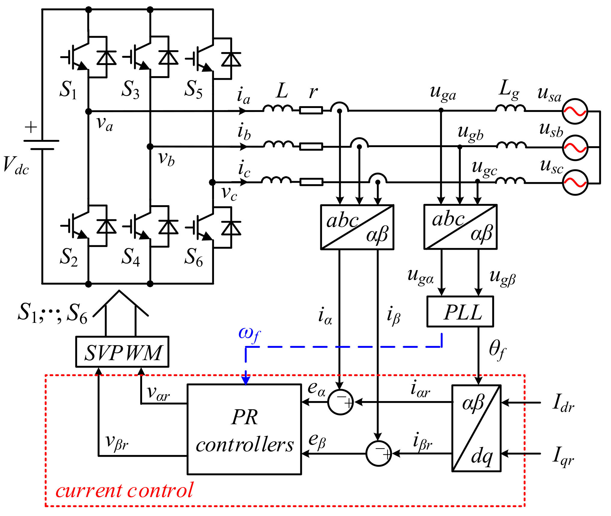
Figure 3.
Detailed block diagrams of adaptive PR controllers with different implementations of R(s).
Figure 3.
Detailed block diagrams of adaptive PR controllers with different implementations of R(s).
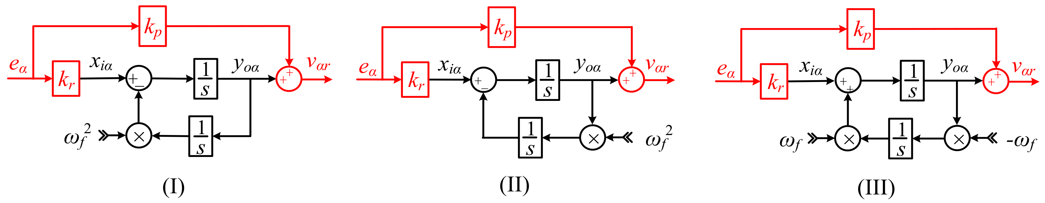
Figure 4.
Block diagram of (a) a basic synchronous reference frame PLL (SRF-PLL); (b) a dual second order generalized integrator frequency locked loop (DSOGI-FLL) based grid synchronization with frequency locked loop (FLL) gain normalization.
Figure 4.
Block diagram of (a) a basic synchronous reference frame PLL (SRF-PLL); (b) a dual second order generalized integrator frequency locked loop (DSOGI-FLL) based grid synchronization with frequency locked loop (FLL) gain normalization.
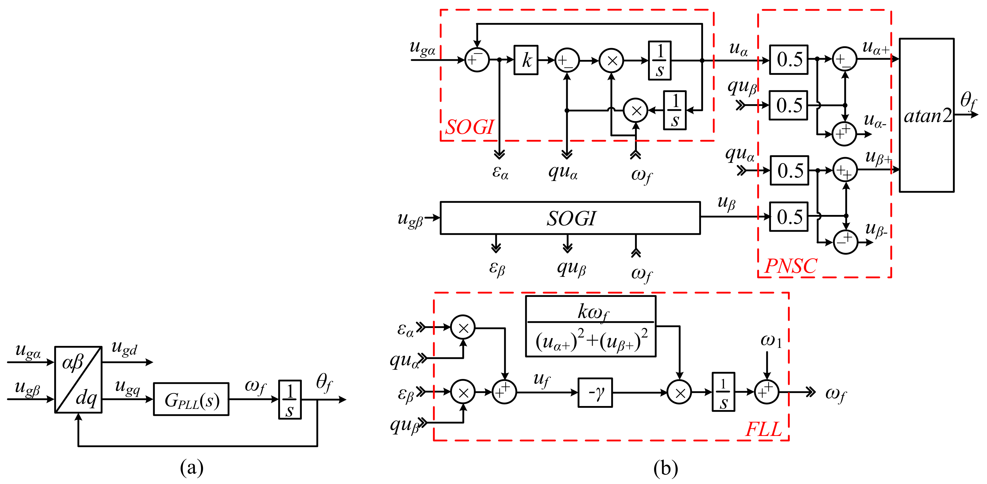
Figure 5.
Small signal model of grid current control loop influenced by the PLL system.
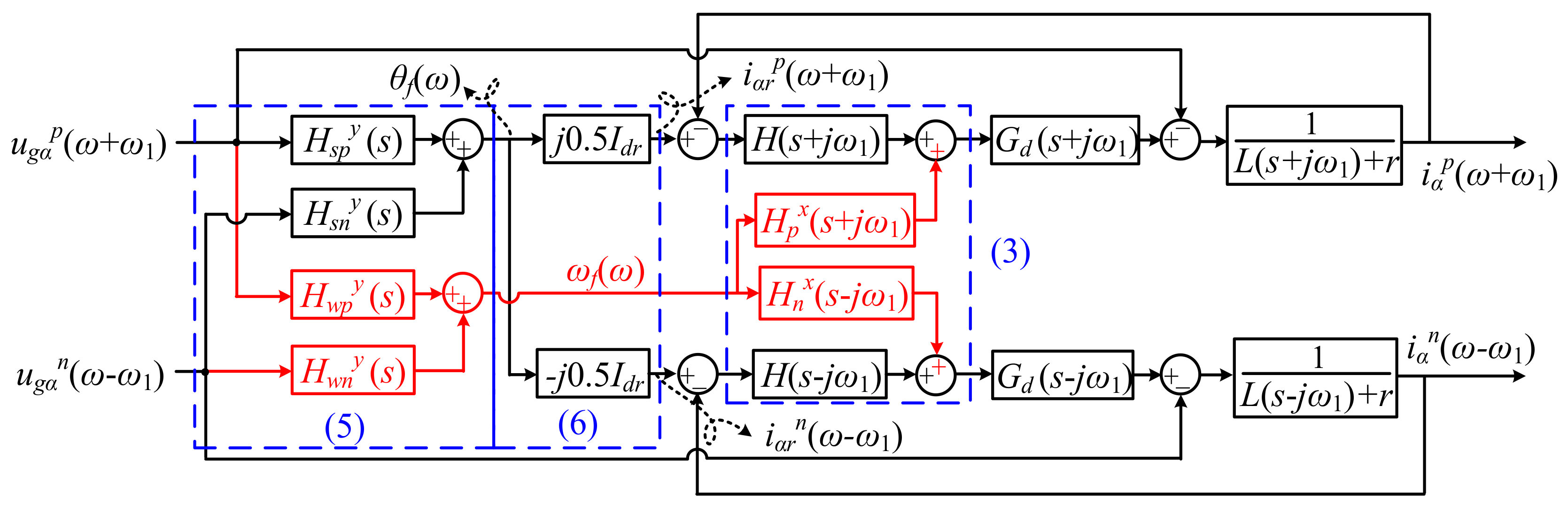
Figure 6.
Magnitude responses of admittances of the converter synchronized by a SRF-PLL: (a) Ypp(s + jω1); (b) Ypn(s + jω1); (c) Ynp(s − jω1); (d) Ynn(s − jω1). Red line: Implementation I; Green line: implementation II; Black line: implementation III is applied. Circles: numerical simulation results.

Figure 7.
Magnitude responses of admittances of the converter synchronized by a DSOGI-FLL: (a) Ypp(s + jω1); (b) Ypn(s + jω1); (c) Ynp(s − jω1); (d) Ynn(s − jω1). Red line: Implementation I; Green line: implementation II; Black line: implementation III is applied. Circles: numerical simulation results.

Figure 8.
Nyquist curves of characteristic loci of Lαβ with different implementations of the adaptive resonance controllers using (a) DSOGI-FLL; (b) SRF-PLL for grid synchronization. Solid line: λ1(s); Dash line: λ2(s).
Figure 8.
Nyquist curves of characteristic loci of Lαβ with different implementations of the adaptive resonance controllers using (a) DSOGI-FLL; (b) SRF-PLL for grid synchronization. Solid line: λ1(s); Dash line: λ2(s).
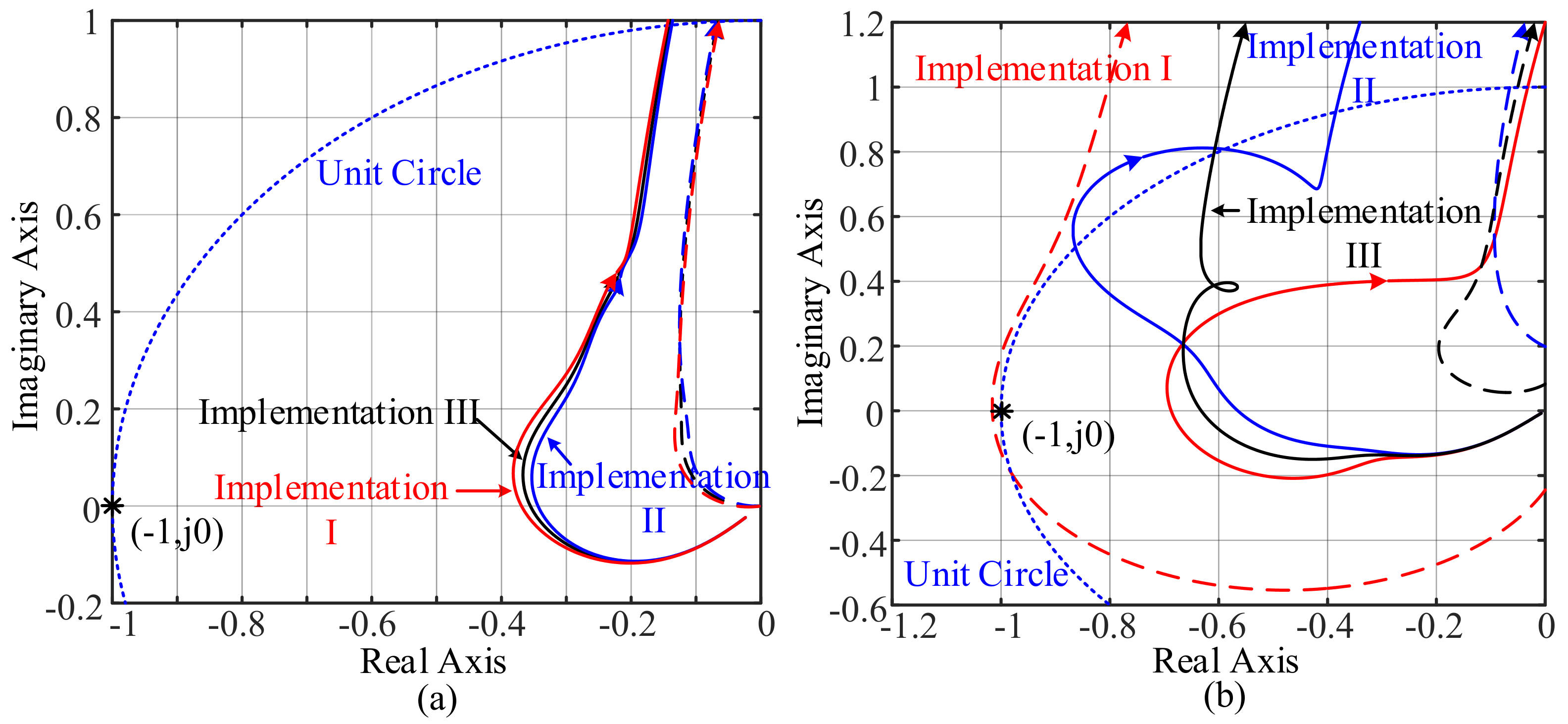
Figure 9.
Stability boundaries of the grid-connected converter using different implementations of the adaptive PR controller and SRF-PLL for grid synchronization.
Figure 9.
Stability boundaries of the grid-connected converter using different implementations of the adaptive PR controller and SRF-PLL for grid synchronization.
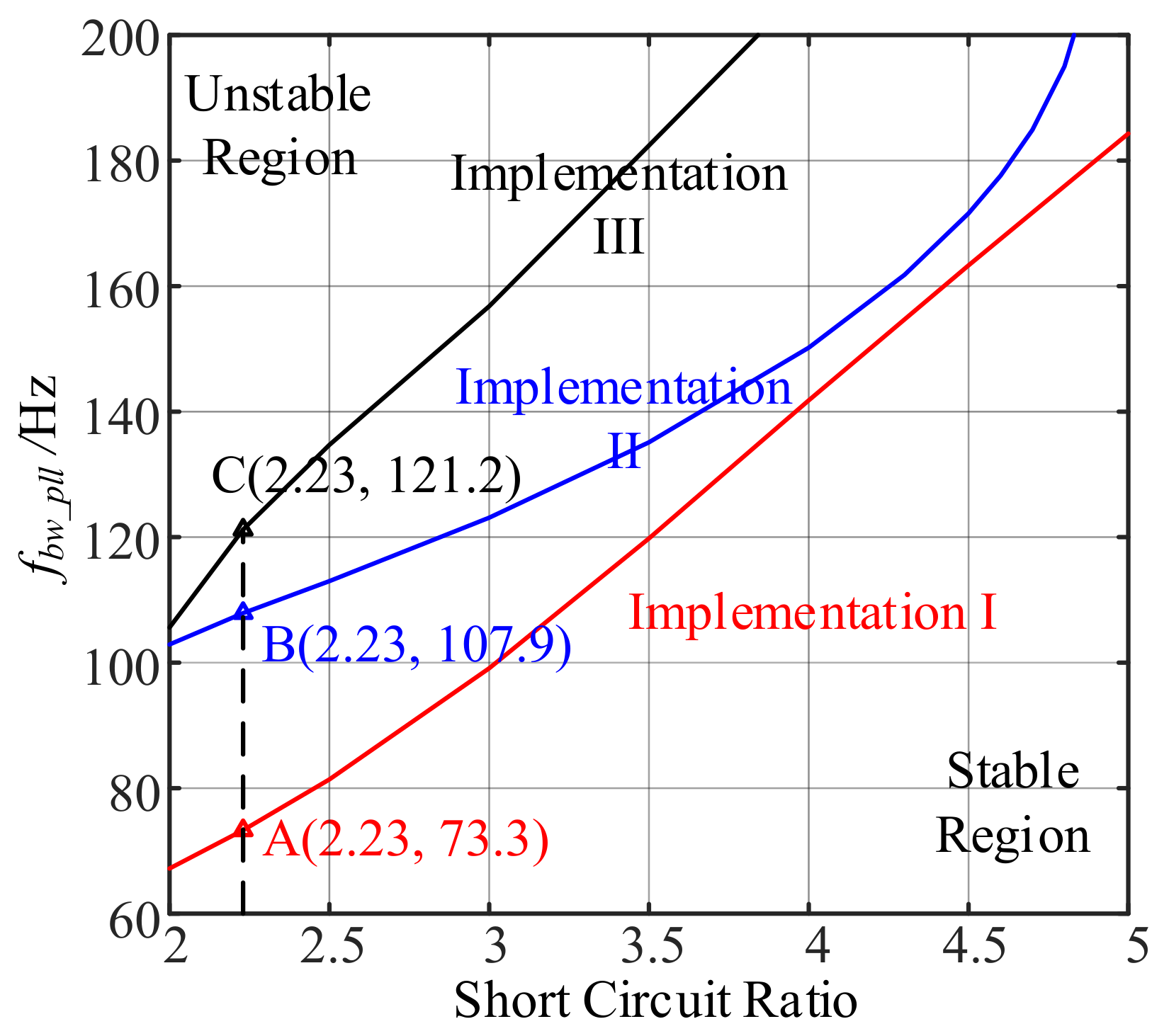
Figure 10.
Frequency response of the effects of point of common coupling (PCC) voltages on θf in (a) and ωf in (b). Solid line: DSOGI-FLL is used; Dash line: SRF-PLL is used.
Figure 10.
Frequency response of the effects of point of common coupling (PCC) voltages on θf in (a) and ωf in (b). Solid line: DSOGI-FLL is used; Dash line: SRF-PLL is used.
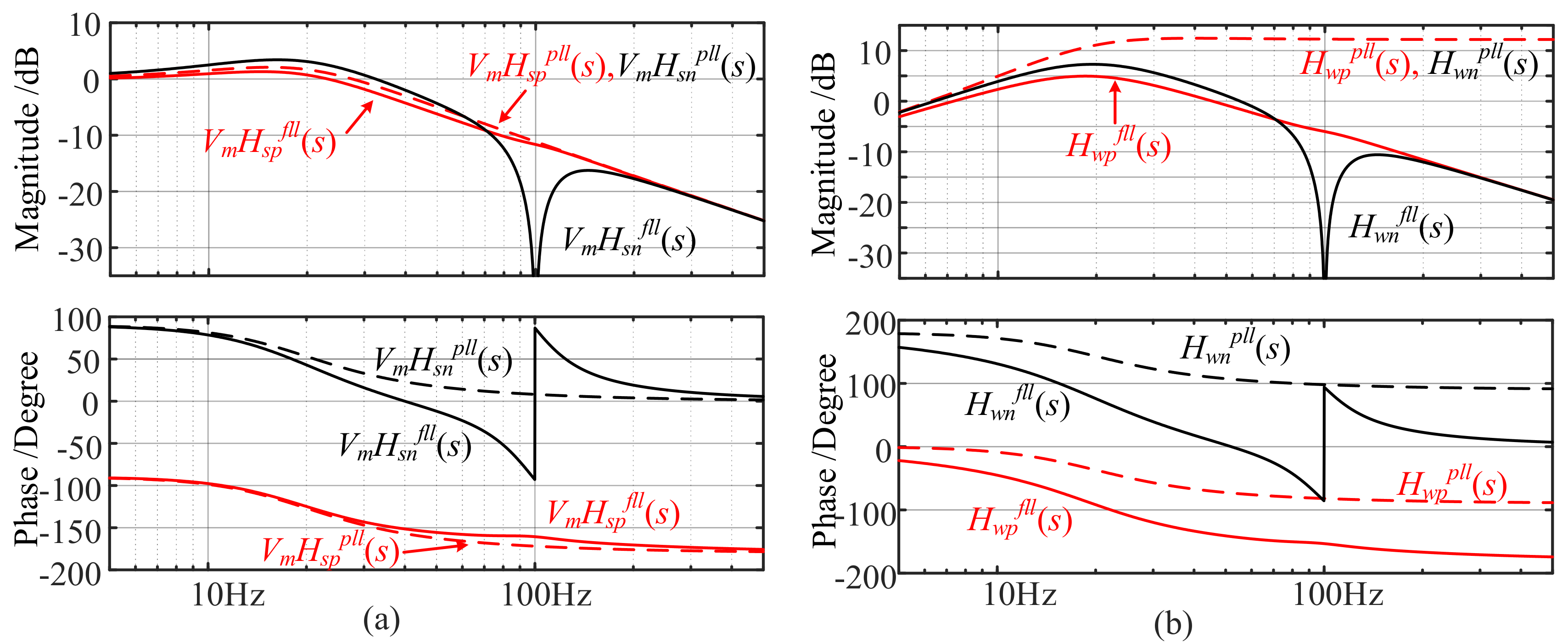
Figure 11.
Nyquist curves of characteristic loci of Lαβ using different PLLs. Black line: SRF-PLL; Red line: DSOGI-FLL is used. Solid line: λ1(s); Dash line: λ2(s).
Figure 11.
Nyquist curves of characteristic loci of Lαβ using different PLLs. Black line: SRF-PLL; Red line: DSOGI-FLL is used. Solid line: λ1(s); Dash line: λ2(s).

Figure 12.
A-phase current waveforms for the converter using (a) implementation I; (b) implementation II; (c) implementation III of the adaptive resonance controllers with fbw_pll changes at time T0.
Figure 12.
A-phase current waveforms for the converter using (a) implementation I; (b) implementation II; (c) implementation III of the adaptive resonance controllers with fbw_pll changes at time T0.

Figure 13.
Dynamic responses of the converter using (a) implementation I; (b) implementation II; (c) implementation III of the adaptive resonance controllers with changing active current reference.
Figure 13.
Dynamic responses of the converter using (a) implementation I; (b) implementation II; (c) implementation III of the adaptive resonance controllers with changing active current reference.
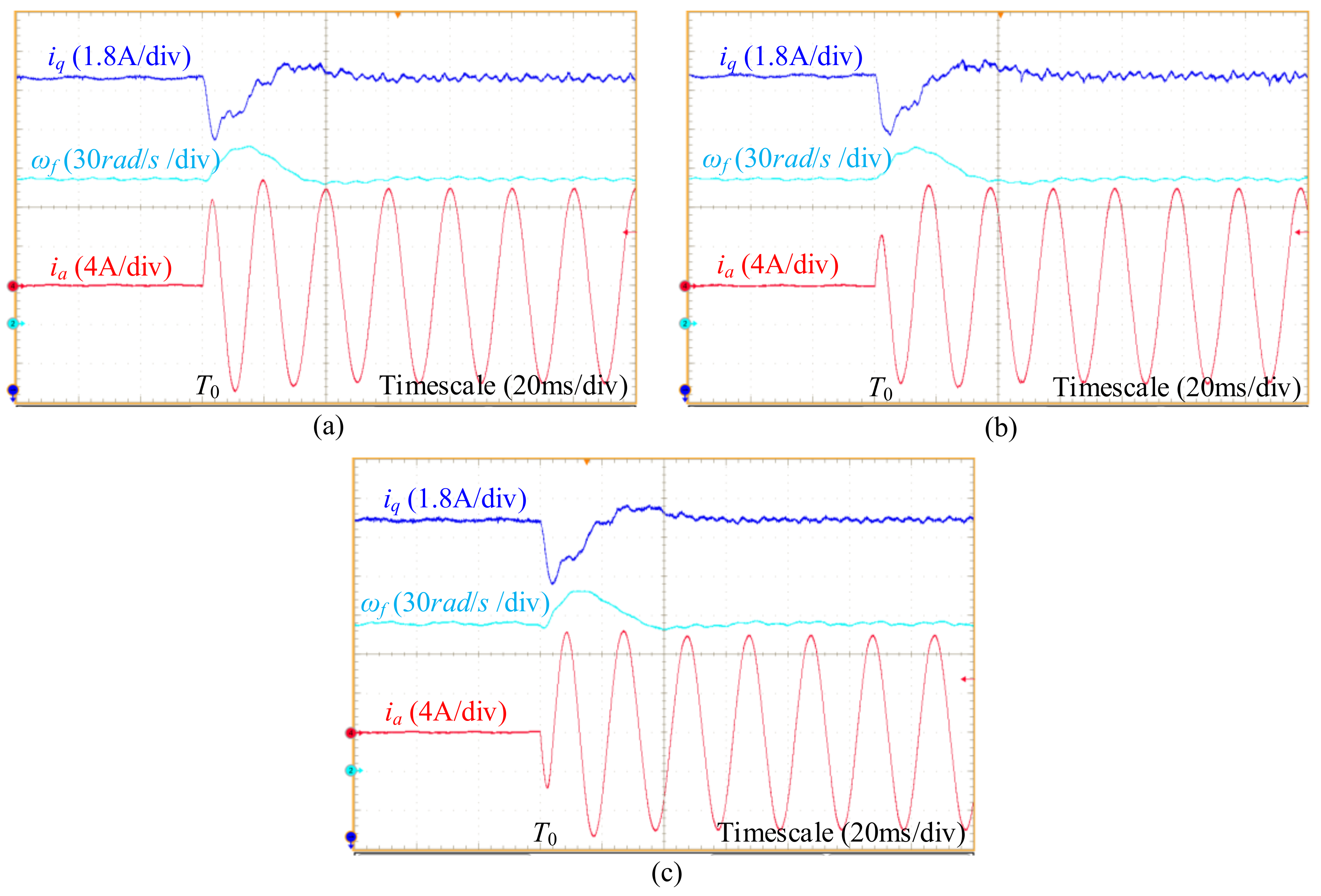
Figure 14.
Dynamic response of q-axis component of grid current with its reference changes from −6 A to 0 A at time T0: (a) SRF-PLL; (b) DSOGI-FLL is used for grid synchronization.
Figure 14.
Dynamic response of q-axis component of grid current with its reference changes from −6 A to 0 A at time T0: (a) SRF-PLL; (b) DSOGI-FLL is used for grid synchronization.

Table 1.
Detailed expressions of (s) and (s) in Equation (3) with different implementations of the adaptive PR current controllers.
Table 1.
Detailed expressions of (s) and (s) in Equation (3) with different implementations of the adaptive PR current controllers.
| X | i | ii | iii |
|---|---|---|---|
Table 2.
Detailed expressions of the transfer functions in Equation (5) with different phase-locked loops (PLLs).
Table 2.
Detailed expressions of the transfer functions in Equation (5) with different phase-locked loops (PLLs).
Table 3.
Parameters of grid-tied converter prototype.
| Symbol | Description | Value |
|---|---|---|
| V1 | Grid phase-neutral peak voltage | 30√2 V |
| ω1 | Grid angular frequency | 2π × 50 rad/s |
| fs | Switching frequency | 10 kHz |
| Vdc | Dc-link voltage | 130 V |
| L | Inductance of the L-type filter | 2 mH |
| r | Resistance of the filter | 0.2 Ω |
| αc | Current control loop bandwidth | 2π × 833 rad/s |
| ki | Proportional gain of ac/dc current controller | 10.47 |
| kr | R parameter of ac/dc current controller | 1047 |
| Idr | D channel current reference of VSC | 10 A |
© 2018 by the authors. Licensee MDPI, Basel, Switzerland. This article is an open access article distributed under the terms and conditions of the Creative Commons Attribution (CC BY) license (http://creativecommons.org/licenses/by/4.0/).
Share and Cite
MDPI and ACS Style
Li, X.; Lin, H. Stability Analysis of Grid-Connected Converters with Different Implementations of Adaptive PR Controllers under Weak Grid Conditions. Energies 2018, 11, 2004. https://doi.org/10.3390/en11082004
AMA Style
Li X, Lin H. Stability Analysis of Grid-Connected Converters with Different Implementations of Adaptive PR Controllers under Weak Grid Conditions. Energies. 2018; 11(8):2004. https://doi.org/10.3390/en11082004
Chicago/Turabian StyleLi, Xing, and Hua Lin. 2018. "Stability Analysis of Grid-Connected Converters with Different Implementations of Adaptive PR Controllers under Weak Grid Conditions" Energies 11, no. 8: 2004. https://doi.org/10.3390/en11082004
Note that from the first issue of 2016, this journal uses article numbers instead of page numbers. See further details here.