Multi-Step Ahead Wind Power Generation Prediction Based on Hybrid Machine Learning Techniques

Abstract

Accurate generation prediction at multiple time-steps is of paramount importance for reliable and economical operation of wind farms. This study proposed a novel algorithmic solution using various forms of machine learning techniques in a hybrid manner, including phase space reconstruction (PSR), input variable selection (IVS), K-means clustering and adaptive neuro-fuzzy inference system (ANFIS). The PSR technique transforms the historical time series into a set of phase-space variables combining with the numerical weather prediction (NWP) data to prepare candidate inputs. A minimal redundancy maximal relevance (mRMR) criterion based filtering approach is used to automatically select the optimal input variables for the multi-step ahead prediction. Then, the input instances are divided into a set of subsets using the K-means clustering to train the ANFIS. The ANFIS parameters are further optimized to improve the prediction performance by the use of particle swarm optimization (PSO) algorithm. The proposed solution is extensively evaluated through case studies of two realistic wind farms and the numerical results clearly confirm its effectiveness and improved prediction accuracy compared to benchmark solutions.

1. Introduction

Currently, the urgent pursuit of low-carbon economy and advances of wind power technologies are strongly driving the rapid sustainable transition in the energy sector as well as the wind power development across the world [1,2]. Due to the intermittent and stochastic nature, the power generation of wind farms needs to be accurately predicted at different time-scales (e.g., daily, hourly or even less) and timely reported to the dispatch center. Accurate short-term wind power forecasting can improve wind power utilization, increase system reliability, reduce operational cost nd allow flexible dispatch strategies [3]. In particular, the ultra-short-term wind power prediction for a couple of hours ahead with the small prediction cycle (e.g., 15 min) can provide strong support for frequency modulation and spinning reserve optimization. However, such ultra-short-term prediction is often a non-trivial task that demands advanced algorithmic solutions and tools with sufficient accuracy and acceptable computational complexity.

In the literature, much research effort has been made to address the prediction issues from different aspects, e.g., electricity pricing [4,5] and power generation [6], in energy systems. The available prediction tools and solutions of ultra-short-term prediction can be categorized into three classes: physical-based methods, statistical-based methods, and machine learning-based methods. The physical-based methods focus on the spatial and temporal factors in a full fluid-dynamics atmosphere model [7], which can generally perform well in longer horizons. The statistical-based methods, e.g., autoregressive model (AR), moving-average (MA), auto-regressive integrated moving average (ARIMA) and Kalman filters, carry out statistical analysis based on the historical data to identify the internal regularity and the tendency of variations to deduce the prediction results. The machine learning-based methods include several supervised learning models, e.g., artificial neural networks (ANNs) [8], support vector machines (SVMs) [9], adaptive neuro-fuzzy inference systems (ANFISs) [10] and Gaussian processes (GPs) [11]. In addition, some combined or hybrid methods have been proposed aim to improve the prediction performance. For example, a hybrid intelligent method was proposed in [3] using multiple support vector regression (SVR) models with the parameters estimated based on an enhanced harmony search (EHS) algorithm. In [12], a hybrid forecasting model based on K-means clustering and an a priori algorithm was developed for short-term wind speed prediction and the prediction errors are corrected by associated rules.

In recent years, the feature selection and analysis of machine-learning based models for wind power prediction have received much attention. The prediction accuracy can be improved by exploring the information obtained from of the historical wind speed and generation time series data. In [13], the features are firstly extracted from the historical power generation data, and then the dataset is split into subsets based on the stationary patterns. In [14], a novel decomposition approach to fully consider the chaotic nature of wind power time series was proposed. The time series data were separated into different frequency characteristics using ensemble empirical mode decomposition (EMD) before carrying out the chaotic time series analysis and singular spectrum analysis (SSA). A forecasting model combining a support vector machine (SVM) optimized by a genetic algorithm and feature selection based on the phase space reconstruction was presented in [15] for short-term wind speed prediction. In addition, numerical weather prediction (NWP) data (including wind speed, direction, temperature, humidity, atmospheric pressure, etc.) were adopted as the input variables for supervised models. In [16], output data from different NWP models were used and the data with the minimum training error were selected to be used in both ANN and SVM models. Afterwards, the forecasting errors were corrected based on the model output statistics (MOS). The study in [17] proposed a wind power prediction model based on the composite covariance function considering the joint effects among features of NWP data. In [18], a data-driven feature extraction approach was developed to utilize unlabeled NWP data which can be used in the supervised forecasting models.

It should be noted that, as the dimensionality of input variable increases, irrelevant and redundant variables can deteriorate the prediction performance. Therefore, the selection of appropriate variables through dimensionality reduction approaches is needed [19], and two dimensionality reduction techniques, feature selection (variable selection) and feature extraction (feature transform), are often used [20]. The latter can produce a new feature space through mapping the original features into lower dimensional ones, e.g., singular value decomposition (SVD), principal component analysis (PCA) and locally linear embedding (LLE). However, such feature extraction methods may often lose physical properties of the original variables, and also difficult to be interpreted. In time series data analysis, the variable selection that filters out some meaningless attributes without any transformation can be more attractive than feature extraction. The variable selection methods can select the compact subset from the original dataset to improve the performance and interpretability of the prediction model.

In general, three types of feature selection methods, filter methods, wrapper methods and embedded methods, are considered [21]. The filter method ranks the input variables with a correlation or mutual information (MI) criteria and selects the variable with the highest ranking. It is effectively a pre-processing step before the development of the predictive model [21]. The wrapper method identifies and evaluates the subsets of input variables based on the accuracy contributed by the given output variable. Similarly, the embedded one builds the close-loop search into a classifier construction in the training process [22]. The wrapper and embedded techniques can generally achieve better accuracy than the filter technique, but the filter method is less likely to lead to over-fitting and with less computational complexity [23].

It should be highlighted that the existing solutions either have not been able to fully consider the available information (e.g., historical data and NWP) or select the appropriate variables for improving the prediction accuracy. To the author’s best knowledge, the technical challenge of ultra-short-term prediction of wind power generation remains and the hybrid approach based on data mining and machine learning techniques has not been thoroughly exploited.

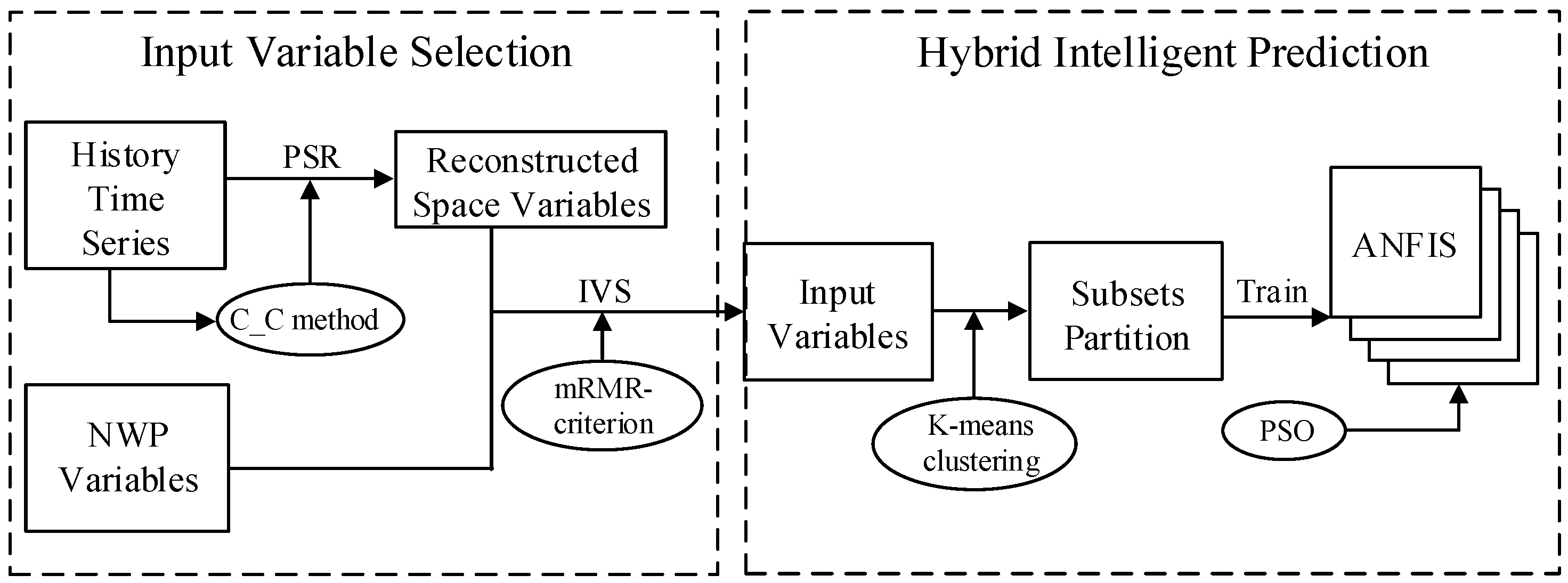
This paper attempts to address the challenge of ultra-short-term power generation prediction in wind farms. The main technical contributions made in this work are summarized as follows: a novel hybrid algorithmic solution is presented which considers both historical generation data and NWP data, and selects the optimal combination of input features using a filter method for different prediction steps. The proposed algorithmic solution was extensively evaluated and validated through case studies of two realistic wind farms. The basic idea behind the proposed prediction solution is illustrated in Figure 1. The long-term nonlinear dynamic characteristics of wind power time series data are extracted and recovered by using phase space reconstruction in C_C method. Afterwards, the most appropriate input variables are selected from the reconstructed phase and NWP features with respect to different forecasting steps based on the minimal redundancy and maximal relevance criterion. Finally, an adaptive neuro-fuzzy inference system based algorithmic solution with heuristically optimized parameters is adopted by using the selected input variables to produce the prediction results.

The rest of this paper is organized as follows: Section 2 describes the input variable selection (IVS) solution based on (PSR) technique and mRMR criterion. Section 3 presents the framework of the proposed hybrid intelligence prediction model. Section 4 carries out the case studies and presents a set of key numerical results. Finally, the conclusions are given in Section 5.

2. Input Variable Selection (IVS)

Due to the chaotic property of the weather system, the evolution of dynamic characteristics has initial sensitivity. The correlation between historical time series and future wind power generation will decay rapidly with the increase of forecasting time step, and even deteriorate the prediction performance. Thus, the adoption of both historical generation data and the numerical weather prediction (NWP) data as the input variables is required. NWP aims to predict the variation of weather through solving the process of thermodynamics and hydrodynamics equations based on the meteorological data of the system. However, it can only provide short-term surface wind and other weather characteristics prognoses roughly, which are not entirely adequate for specific local conditions [24]. NWP data are often adopted to provide ancillary information, e.g., wind speed, wind direction, temperature, humidity and air pressure, for prediction. For different step-ahead prediction, these input variables can have different impacts on the forecasting targets. Therefore, a two-stage input variable selection is used in the proposed prediction solution. Firstly, the initial variables can be selected from the historical series data through the phase space reconstruction technique (PSRT), and the initial variables further can be combined with NWP information as the candidate inputs. Secondly, the optimal input variables are filtered based on mRMR criterion.

2.1. The Initial Input Variable Selection of Historical Series Using PSRT

The Lyapunov exponent can be used to prove that the wind power generation time series has chaotic characteristics. Therefore, the nonlinear dynamic characteristics of wind power time series can be extracted and recovered by using phase space reconstruction theory. In [25], the time-delay technique was used to reconstruct a finite dimensional phase space of sampled system’s time evolution. In the time delay coordinate reconstruction, it is not only very important but also difficult to choose an appropriate time delay τ and a good embedding dimension m since real datasets are finite and noisy. There are currently two different viewpoints for the estimation of the aforementioned parameters. One holds that they are irrelevant and should be chosen independently. To choose time delay τ, one can use methods including autocorrelation function, multiple-autocorrelation, mutual information, and so on. G-P algorithm or False Nearest Neighbor can be used to find the embedding dimension m. However, it is suggested that the delay time and embedding dimension are dependent mutually. The delay time window $\varpi$ should be estimated for the choice of m and τ. The delay time window $\varpi$ can be estimated using C_C method [26]. The C_C method was used to determine the optimal input variables form the historical generation with reduced computational complexity and enhanced efficiency [27].

The phase space reconstruction is an efficient tool to analyze the dynamic pattern of a chaotic time series data. The delay-coordinate method was presented by Takens et al. to perform the phase space reconstruction. The time series $x=\left\{x_i,i=1,2,\dots ,N\right\}$ can be reconstructed into a multi-dimensional phase space $X=\left\{X_i\right\}$ to represent the dynamic system, according to:

$$X_i=\left[x_i,x_{i+\tau },\dots ,x_{i+\left(m-1\right)\tau }\right]$$

(1)

where $i=1,2,\dots ,M$, $M=N-\left(m-1\right)\tau$, $m$ is the embedding dimension, and $\tau$ is the delay time. In this study, the C_C method [26] was constructed via two correlation integrals, developed to reconstruct the given time series $x=\left\{x_i\right\}$ to simplify the candidate input forms.

As suggested in [26], the correlation integral for the embedded time series is defined as:

$$C\left(m,N,r,t\right)=\frac{2}{M\left(M-1\right)}{\displaystyle \sum _{1\le i\le j\le M}\theta \left(r-d_{ij}\right)}, r>0$$

(2)

where $d_{ij}={\Vert x_i-x_j\Vert }_{\infty }$, ${\Vert ·\Vert }_{\infty }$ represents the infinite norm, $t$ denotes the index lag, and $\theta$ is the Heaviside function, $\theta \left(x\right)=\{\begin{array}{c}0, x<0\\ 1, x\ge 0\end{array}$. The correlation integral is a cumulative distribution function, which denotes the probability with the distance less than search radius $r$ between any two points in the phase space. To study the nonlinear dependence and eliminate spurious temporal correlations, the given time series $x=\left\{x_i\right\}$ must be divided into $t$ disjoint sub-sequences. The disjoint time series can be expressed as (3):

$$\begin{array}{c}\left\{x_1,x_{1+t},\dots ,x_{1+\left(l-1\right)t}\right\}\\ \left\{x_2,x_{2+t},\dots ,x_{2+\left(l-1\right)t}\right\}\\ \cdots \cdots \\ \left\{x_t,x_{2t},\dots ,x_{lt}\right\}\end{array}$$

(3)

where $l$ is the length of subseries, $l=INT\left(N/t\right)$, and $INT(·)$ denotes reserving integer of the value.

Let us construct a statistic function $S\left(m,N,r,t\right)$ as the serial correlation of a nonlinear time series, which is a dimensionless measure of nonlinear dependence. For general t in the above disjoint time series expressed in Equation (3), $S\left(m,N,r,t\right)$ is defined as Equation (4):

$$S\left(m,N,r,t\right)=\frac{1}{t}{\displaystyle \sum _{s=1}^t\left[C_s\left(m,\frac{N}{t},r,t\right)-C_s^m\left(1,\frac{N}{t},r,t\right)\right]}$$

(4)

Finally, when $N\to \infty$, the following can be obtained:

$$S\left(m,r,t\right)=\frac{1}{t}{\displaystyle \sum _{s=1}^t\left[C_s\left(m,r,t\right)-C_s^m\left(1,r,t\right)\right]}$$

(5)

If the time series data follows an independent and identical distribution, $S\left(m,r,t\right)$ is equal to zero constantly for fixed value m, t and $N\to \infty$. However, as the real dataset is finite and the components of series are correlated, $S\left(m,r,t\right)$ is non-zero [26]. The maximum deviation of $S\left(m,r_j,t\right)$ for all radius r can be defined as (6):

$$\Delta S\left(m.t\right)=\max \left\{S\left(m,r_j,t\right)\right\}-\min \left\{S\left(m,r_j,t\right)\right\}$$

(6)

Here, N, m and r can be estimated based on the Brock–Dechert–Scheinkman (BDS) statistics as $N=3000$, $m=2,3,4,5$, $r_i=i\sigma /2, i=1,2,3,4$, respectively, where $\sigma =std\left(x\right)$ denotes the standard deviation of the time series. Then, Equations (7)–(9) can be obtained as:

$$\overline{S}\left(t\right)=\frac{1}{16}{\displaystyle \sum _{m=2}^5{\displaystyle \sum _{j=1}^{4}S\left(m,r_j,t\right)}}$$

(7)

$$\Delta \overline{S}\left(t\right)=\frac{1}{4}{\displaystyle \sum _{m=2}^5\Delta S\left(m,t\right)}$$

(8)

$$S_{cor}\left(t\right)=\Delta \overline{S}\left(t\right)+\left|\overline{S}\left(t\right)\right|$$

(9)

The optimal delay time $\tau$ is determined when the value of $\overline{S}\left(t\right)$ first reaches zero or when $\Delta \overline{S}\left(t\right)$ reaches the first minimum point. The optimal embedding window $\varpi$ corresponds to the global minimum point of $S_{cor}$. Furthermore, the embedding dimension m can be obtained by the following formula: $m=\varpi /\tau +1$.

Once the reconstruction parameters, delay time $\tau$ and embedding dimension m, are determined by C_C method, the initial variables related to the historical sequence are obtained as $Hi{s}_{Inputs}\left(t\right)=\left[x\left(t\right),x\left(t-\tau \right),\dots ,x\left(t-\left(m-1\right)\tau \right)\right]$, where $x\left(t\right)$ is the power generation values observed at current time t. The forecasting weather variables provided by NWP can be written as $NW{P}_{Inputs}\left(t^{\prime }\right)=\left[V_{wind}\left(t^{\prime }\right),\left(\sin \left(D_{wind}\left(t^{\prime }\right)\right)+\cos \left(D_{wind}\left(t^{\prime }\right)\right)\right),T\left(t^{\prime }\right),H\left(t^{\prime }\right),P\left(t^{\prime }\right)\right]$, where $V_{wind}\left(t^{\prime }\right)$, $D_{wind}\left(t^{\prime }\right)$, $T\left(t^{\prime }\right)$, $H\left(t^{\prime }\right)$ and $P\left(t^{\prime }\right)$ in turn represent wind speed, wind direction, temperature, humidity and air pressure at the predicted time $t^{\prime }$. Therefore, candidate input variables set can be combined into $V=\left[Hi{s}_{Inputs}\left(t\right),NW{P}_{Inputs}\left(t^{\prime }\right)\right]$, and the input set dimension is $\left|V\right|=m+5$.

2.2. The Optimal Selection of Candidate Input Variables Using mRMR-Criterion Ranking

The input variables of historical generation and NWP are selected using the minimal redundancy maximal relevance (mRMR) criterion based on mutual information (MI) [28]. As MI can measure both the linear and nonlinear dependency between variables, it has been applied for correlation measurement and variable selection [29]. The basic idea of variable selection algorithm based on MI is to select the best subset $S$ from the original dataset $X$ by maximizing the joint MI between $S$ and target output $Y$, namely $I\left(S;Y\right)$. In the literature, many MI-based variable selection algorithms are available, e.g., mutual information feature selection (MIFS) [30], mutual information feature selection under uniform information distribution (MIFS-U) [31], the minimal redundancy maximal relevance (mRMR) [28], and normalized mutual information feature selection (NMIFS) [32]. In this work, the mutual-information-based mRMR criterion is adopted to find the compact and informative input space. The mRMR technique aims to find a subset of candidate variables with maximal dependency (with respect to the target to be predicted) as well as minimal redundancy (between the variables in the subset). The concept of MI is based on entropy that is described as follows.

The entropy of a random variable indicates the required average amount of information to describe the random variable [33] which has been adopted in many studies [34,35]. The entropy of a discrete random variable $X=\left(x_1,x_2,\dots ,x_N\right)$ is denoted by $H\left(X\right)$, where $x_i$ refers to the possible values that X can take for discrete variable or the possible value range for continuous variable. $H\left(X\right)$ is defined as:

$$H\left(X\right)=-{\displaystyle \sum _{i=1}^{N}p\left(x_i\right)\log \left(p\left(x_i\right)\right)}$$

(10)

where $p\left(x_i\right)$ is the probability mass function.

For any two random variables, $X$ and $Y=\left(y_1,y_2,\dots ,y_M\right)$, the joint entropy is defined as:

$$H\left(X,Y\right)=-{\displaystyle \sum _{j=1}^M{\displaystyle \sum _{i=1}^{N}p\left(x_i,y_j\right)\log \left(p\left(x_i,y_j\right)\right)}}$$

(11)

where $p\left(x_i,y_j\right)$ is the joint probability mass function of $X$ and $Y$. The conditional entropy of $X$ given $Y$ is defined as:

$$H\left(Y|X\right)=-{\displaystyle \sum _{j=1}^M{\displaystyle \sum _{i=1}^{N}p\left(x_i,y_j\right)\log \left(p\left(y_j|x_i\right)\right)}}$$

(12)

The conditional entropy is the amount of uncertainty left in $Y$ when a variable $X$ is introduced, so it is less than or equal to the entropy of both variables. The conditional entropy is equal to the entropy if, and only if, the two variables are independent. Mutual Information (MI) is the amount of information that both variables share, and is defined as:

$$I\left(X;Y\right)=H\left(Y\right)-H\left(Y|X\right)$$

(13)

MI can be expressed as the amount of information provided by variable $X$, which reduces the uncertainty of variable $Y$. MI is zero if the random variables are statistically independent. MI is symmetric, so:

$$I\left(X;Y\right)=I\left(Y;X\right)$$

(14)

The minimal-redundancy-maximal-relevance criterion (mRMR) aims to identify a compact subset of informative input variables by simultaneously considering the maximum relevance scheme and minimum redundancy. The simple combination of individually informative input variables does not necessarily achieve a good forecasting performance [28]. Therefore, both the informativeness of individual input variables and redundancy between them should be considered. Thus, the informativeness score for individual variable $v_i$ based mRMR criterion is given by:

$$J\left(v_i,S\right)=I\left(v_i;t\right)-\frac{1}{\left|S\right|}{\displaystyle \sum _{v_j\in S}I\left(v_i;v_j\right)}\hspace{1em}{v}_i\in \left(V-S\right)$$

(15)

where $V$ is the total candidate variables, $S$ is the selected input variables, and $\left| · \right|$ is the number of variables. The mutual information $I\left(v_i;t\right)$ is used between the target $t$ and the candidate input variable $v_i$ to measure the strength of $v_i$ relative to the forecasting process. The goal of second item is to optimally select those variables that reveal a minimum of resemblance or redundancy between them, thus making the selected set more representative or informative of the whole set.

In the implementation, a stepwise search, incremental forward selection (IFS) method, is used to select input variables according to Equation (15), in which greater $J\left(v_i,S\right)$ scores indicate more promising input variable $v_i$. In the first step, Max-Relevance score of all candidate input variable is calculated, where the variable with the maximum $I\left(v_i;t\right)$ score is determined as the first promising input variable:

$$v_1=\arg \underset{v_i\in V}{\max }I\left(v_i;t\right)$$

(16)

The rest of the variables are selected step by step according to the criterion in Equation (15). In step $m$ ($2\le m\le \left|V\right|$), it is supposed that an input variable subset $S_{m-1}$, composed of $m-1$ promising variables, $s_1,s_2,\dots ,s_{m-1}$, that has been selected from previous step (e.g., step $m-1$). The $m-\mathrm{th}$ promising variable can be selected from $V-S_{m-1}$ at step $m$ by optimizing the following condition:

$$s_m=\arg \underset{v_i\in V-S_{m-1}}{\max }J\left(v_i,S_{m-1}\right)$$

(17)

As one input variable represents one step forward, the promising variables can be incrementally retrieved until step $\left|V\right|$ where a total of input variables $V$ are selected. The variables are also ranked in selection process and the informativeness score (InSc) in $m-\mathrm{th}$ step is given by:

$$InS{c}_m=J\left(s_m,S_{m-1}\right)\hspace{1em}m=2,3,\dots ,\left|V\right|$$

(18)

where $s_m$ is the most promising variable to be selected in $m-\mathrm{th}$ step according to Equation (17). Thus, the priority of candidate input variables can be ranked through the mRMR-based incremental forward selection (IFS) method. The cumulative amount of $InSc$, denoted as $CumInS{c}_m={\displaystyle \sum _{i=1}^{m}InS{c}_i}$, indicates the information contributed from the newly added variable. The final optimal number of input variables can be determined according to the change trend of $CumInSc$.

3. Hybrid Intelligent Prediction Model

In this work, the proposed hybrid algorithmic solution combines the K-means clustering, Particle Swarm Optimization (PSO) and adaptive neuro-fuzzy interference system (ANFIS) in the prediction model.

3.1. Subsets Partition Using K-Means Algorithm

The obtained historical dataset is divided into subsets and the data in the same class are with the similar meteorological features. Consequently, the complexity of network training can be significantly reduced with improved generalization capability. The dataset partitioning is implemented using K-means algorithm as follows.

Here, data centralization and normalization are needed before clustering. Z-score standardization of the dataset is expressed as follows:

$$z_{i,j}=\frac{v_{i,j}-{\mu }_j}{{\sigma }_j}\hspace{1em} i=1,2,\dots N; j=1,2,\dots D$$

(19)

where ${\mu }_j$ is the mean of column $i$, ${\sigma }_j$ is the standard deviation of column, $N$ is the number of instances, and $D$ is the dimensionality of input variables.

Given a training set $\left\{z_1,z_2,\dots ,z_N\right\}$, the K-means clustering algorithmic can partition the dataset into $k$ cohesive groups through an unsupervised learning process [36]. Here, $z_i\in {ℝ}^D$ and first choosing cluster centroids $\left\{a_1,a_2,\dots ,a_k\right\}\in {ℝ}^D$ randomly. Then, the fundamental purpose of K-means algorithm is to minimize the following cost function:

$$C_N=\frac{1}{N}{\displaystyle \sum _{i=1}^N\underset{1\le j\le k}{\min }{\Vert z_i-a_j\Vert }^2}$$

(20)

where $\Vert ·\Vert$ is the function representing the usual Euclidean norm. After determining the cluster center, the training samples are grouped into the subsets of the nearest cluster centers. For $k$ subsets, $U^l=\left\{u_1,u_2,\cdots ,u_{N_l}\right\}$, $l=1,2,\cdots ,k$, the number of samples in each subset is recorded as $N_l, l=1,2,\cdots ,k$. Each subset $U^l$ determines a set of independent ANFIS network parameters during training process. The vector nearest to the cluster center is adopted as the network input when performing the online prediction.

3.2. Adaptive Neuro-Fuzzy Inference System

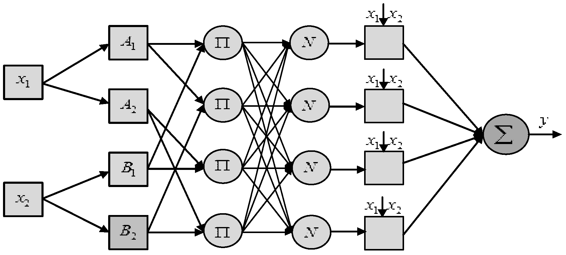
The adaptive neuro-fuzzy interference system (ANFIS) is a data-driven modelling technique [37] to address the multivariable nonlinear system prediction through nonlinear neural network and adaptive fuzzy reasoning process. The fuzzy membership function and fuzzy rules of the system can be obtained through learning from historical data, rather than expert experience or intuition. Figure 2 illustrates the typical structure of two-input ANFIS model. The ANFIS is based on Takagi–Sugeno inference approach that creates a nonlinear mapping from input space to the output space through using the fuzzy if−then rules. The ANFIS is comprised of five layers as follows.

Fuzzifier (Layer 1): Neurons in this layer perform the fuzzification operations, and the membership degree of input in different fuzzy sets (e.g., A1, A2, B1, and B2) can be obtained. Fuzzification is represented by fuzzy membership function $f$, and the output membership degree ${\mu }_A$, ${\mu }_B$ for $x_1$, $x_2$ can be expressed as:

$${\mu }_{Ai}\left(x_1\right)=f\left(x_1\right);\hspace{1em}{\mu }_{Bj}\left(x_2\right)=f\left(x_2\right)\hspace{1em}i,j=1,2$$

(21)

1Rules inference (Layer 2): The rules neurons receive input from their respective fuzzified neurons and calculate the rules active intensity ${\omega }_n$:

$${\omega }_n={\mu }_{Ai}\left(x_1\right){\mu }_{Bj}\left(x_2\right)\hspace{1em}i,j=1,2\hspace{1em}n=1,2,3,4$$

(22)

Normalization (Layer 3): Each neuron in this layer receives all neuronal inputs from the previous layer and calculates the normalized active intensity for a given rule ${\overline{\omega }}_n$:

$${\overline{\omega }}_n={\omega }_n/{\displaystyle \sum {\omega }_n}$$

(23)

Defuzzifier (Layer 4): This layer computes the posteriori value with weight of given rule $f_n$:

$${\overline{\omega }}_n{f}_n={\overline{\omega }}_n\left(p_n{x}_1+p_n{x}_2+r_n\right)$$

(24)

1Output (Layer 5): This layer sums all defuzzified neuron outputs to arrive at the final ANFIS output $y$:

$$y={\displaystyle \sum _n{\overline{\omega }}_n{f}_n}=\frac{{\displaystyle \sum _n{\omega }_n{f}_n}}{{\displaystyle \sum _n{\omega }_n}}$$

(25)

In this work, ANFIS is adopted to fit individual sub-training sets with the parameters heuristically optimized by the use of Particle Swarm Optimization (PSO) algorithm. The structure and parameters of ANFIS are firstly determined using the fuzzy C-Means clustering (FCM) algorithm [38]. Afterwards, PSO is adopted to optimize the parameters. Each particle in PSO can identify and maintain its locally optimal solution (Pbest), and also collectively search for the global optimal solution (Gbest) in the swarm [39]. The location and velocity function in PSO can be expressed as (26).

$$\{\begin{array}{l}{p}_i^d\left(t+1\right)=p_i^d\left(t\right)+v_i^d\left(t+1\right)\\ v_i^d\left(t+1\right)=w\left(t\right)\cdot v_i^d\left(t\right)+c_1{r}_{i1}\cdot \left(pbes{t}_i^d-p_i^d\left(t\right)\right)+c_2{r}_{i2}\cdot \left(gbes{t}^d-p_i^d\left(t\right)\right)\end{array}$$

(26)

where $r_{i1}$ and $r_{i2}$ are two random variables in the range of $\left[0,1\right]$, $c_1$ and $c_2$ are positive constants, and $w$ is the inertia weight. $P_i=\left(p_i^1,p_i^2,\cdots ,p_i^n\right)$ and $V_i=\left(v_i^1,v_i^2,\cdots ,v_i^n\right)$ represents the position and velocity of the $i-\mathrm{th}$ particle, respectively $pbes{t}_i=\left(pbes{t}_i^1,pbes{t}_i^2,\cdots ,pbes{t}_i^n\right)$ and $gbes{t}_i=\left(gbes{t}_i^1,gbes{t}_i^2,\cdots ,gbes{t}_i^n\right)$ represent the best previous position of the $i-\mathrm{th}$ particle and the best previous position among all the particles in the population, respectively.

4. Performance Assessment and Numerical Result

To extensively verify the reliability of the proposed prediction solution, the performance assessment based on the data collected in two real wind farms with different locations and seasons are carried out: Anzishan wind farm (capacity of 45 MW, Henan, China, hub height of 70 m) in June 2017, and Xuqiao wind farm (capacity of 94 MW, Anhui, China, hub height of 90 m) in December 2017. The reference height of these two wind farms is 10 m. The power generation (directly measured) and NWP data with a 15-min interval (e.g., 96 observation values per day) are obtained from these two wind farms. The three-month data (about 8640 observation values) prior to the test month, March to May 2017 and September to November 2017, are used in the training process for Anzishan farm and Xuqiao farm, respectively. The proposed hybrid solution is implemented in the MATLAB (version 8.3, MathWorks, Natick, MA, USA) programming environment.

4.1. Input Variable Selection Process

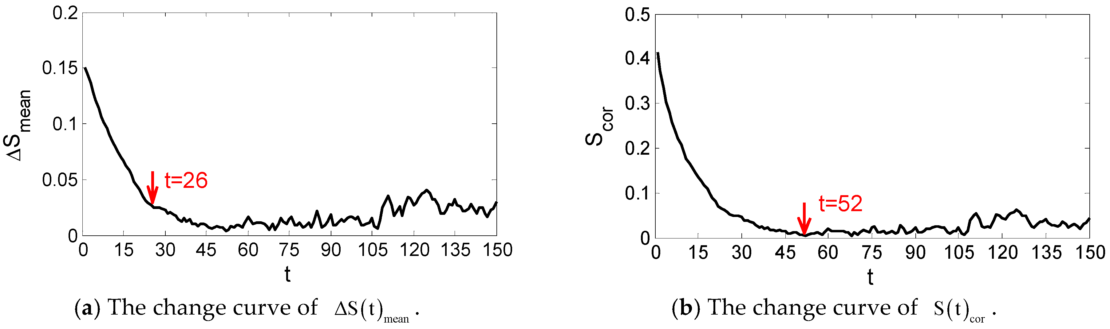
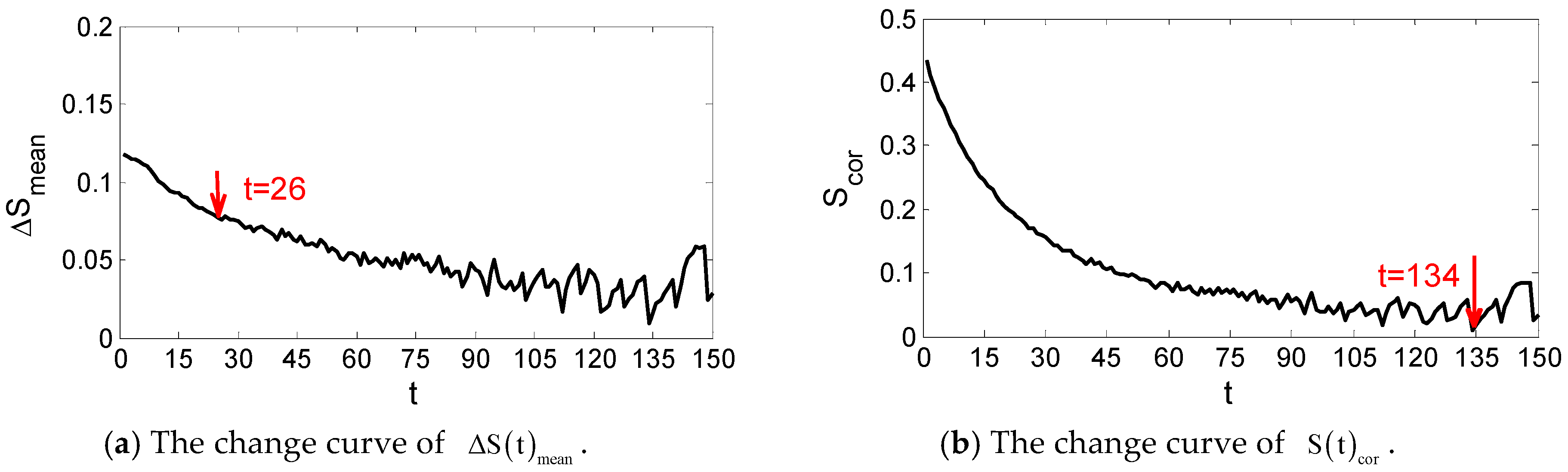
The time series data of power generation in the previous month are used to determine the phase-space reconstruction parameters through the C_C method. With different spatial and temporal characteristics, the parameters of each wind farm will be determined, respectively. For Anzishan farm, it can be observed in Figure 3 that $\Delta \overline{S}$ have the first local minimum when t is equal to 26, thus the optimal delay time $\tau$ is set to 26. The global minimum point of $S_{\mathrm{co}r}$ corresponds to the optimal embedding window $\varpi =52$ as shown in the figure. Thus, the embedding dimension m can be calculated as 3. As for Xuqiao farm, the optimal delay time $\tau$ is also equal to 26 as shown in Figure 4. The embedding window $\varpi$ is observed as 134, thus the optimal embedding dimension m is 6.

The historical time series data can be selected as m-dimension input variables using the phase-space reconstruction. For the current time t, the initial input variables related to the historical data are $Hi{s}_{Inputs}\left(t\right)=\left[x\left(t\right),x\left(t-\tau \right),\dots ,x\left(t-\left(m-1\right)\tau \right)\right]$, where $x\left(t\right)$ is the power generation values observed at current time t. The m-dimensional input variables are in turn denoted as the set: $\left\{Hin1,Hin2,\dots ,Hinm\right\}$. In the same way, the forecasting weather variables provided by NWP data include wind speed, trigonometric wind direction, temperature, humidity, and atmospheric pressure. $NW{P}_{Inputs}\left(t^{\prime }\right)=\left[V_{wind}\left(t^{\prime }\right),\left(\sin \left(D_{wind}\left(t^{\prime }\right)\right)+\cos \left(D_{wind}\left(t^{\prime }\right)\right)\right),T\left(t^{\prime }\right),H\left(t^{\prime }\right),P\left(t^{\prime }\right)\right]$ is in turn denoted as the set: $\left\{windV,windD,Temp,Hum,airP\right\}$. Based on the obtained reconstruction parameters by the C_C method, the candidate input variables set of two wind farms can be obtained as follows:

$$Anzishan: \left\{Hin1,Hin2,Hin3,WindV,WindD,Temp,Hum,AirP\right\}$$

$$Xuqiao: \left\{Hin1,Hin2,Hin3,Hin4,Hin5,Hin6,WindV,WindD,Temp,Hum,AirP\right\}$$

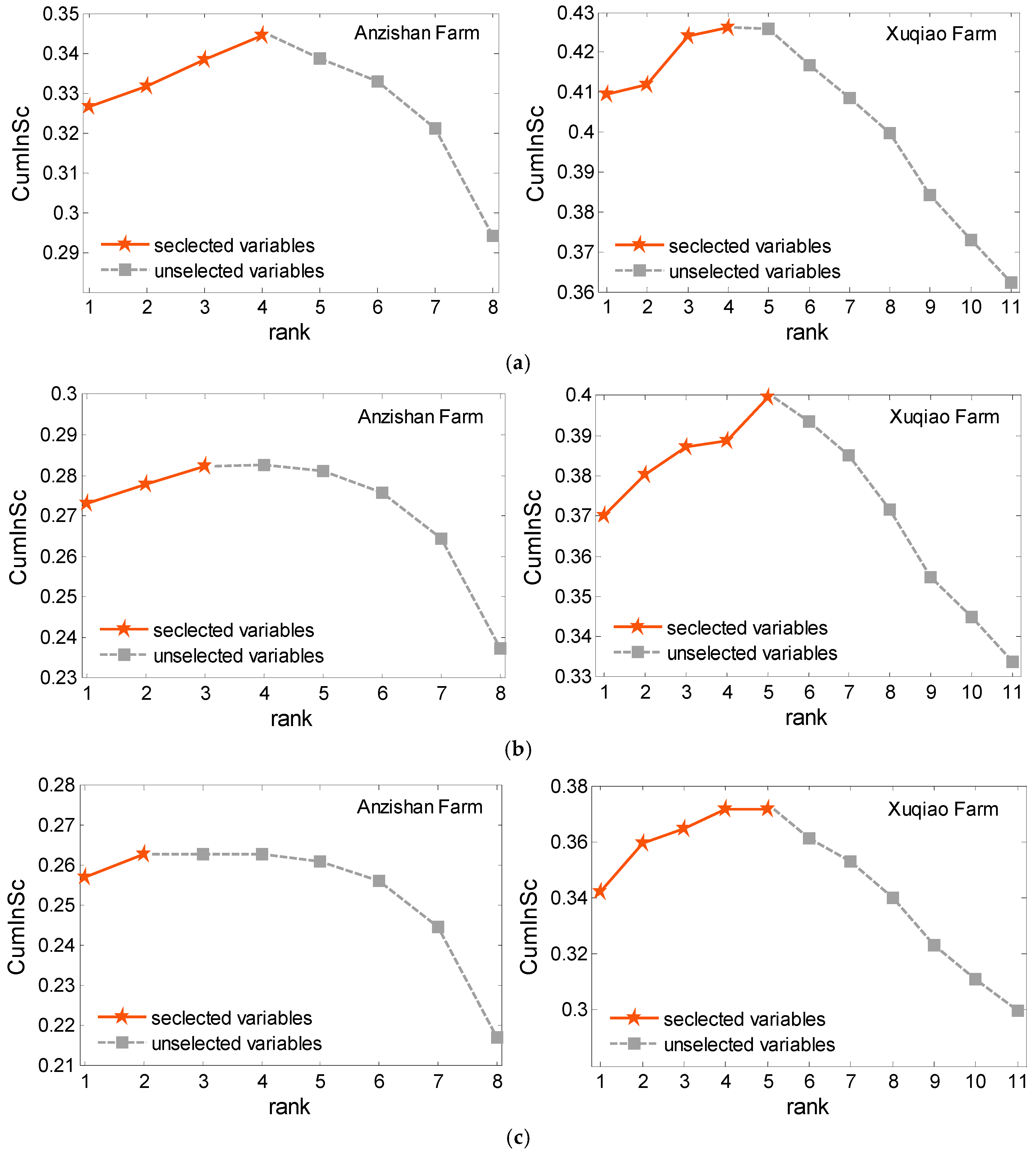
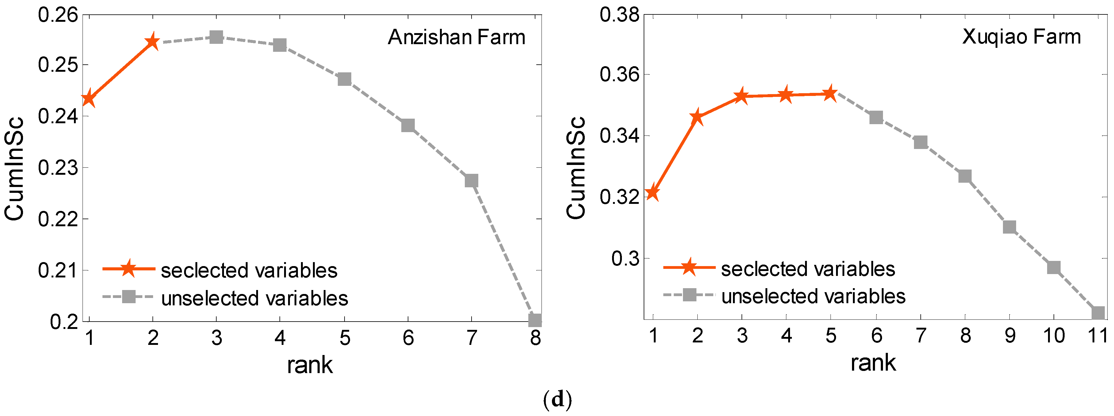
Afterwards, the candidate variables are sorted through mRMR criterion to rank the predictive strength of each input variable. By observing the variation trend of the cumulative amount of $InSc$, that is, when the $CumInSc$ curve no longer increases or grows very slowly, the optimal number of input variables is selected. As the input variable selection is carried out adaptively in the prediction model, the selected input variables may vary for different prediction steps.

Based on proposed mRMR-criterion filter solution, Figure 5 shows the changes of $CumInSc$ curves of Anzishan and Xuqiao wind farms in different predicted steps (e.g., 1 h, 2 h, 3 h and 4 h ahead), respectively. The number of input variables is selected accordingly as shown in Figure 5. In this study, when the $CumInSc$ curve reaches the maxima, it is believed that adding the following variables at the back of extreme point will not add more useful information. Therefore, the candidate variables before the cumulative information maximum are regarded as the optimal or near optimal input variables to the prediction model. The detailed ranking of candidate variables and the number of input choices in multi-step ahead prediction for each farm are shown in

Table 1. Ranking and selection of candidate variables for Anzishan Farm.

Prediction Time Steps (15 min/step)	Input Variables Ranking	Number of Selected Variables
#1	Hin1, WindD, Hin2, WindV; Hin3, Hum, AirP, Temp	4
#2	Hin1, Hin3, WindV, WindD, Hin2; Hum, AirP, Temp	5
#3	Hin1, WindD, WindV, Hin2; Hin3, Hum, AirP, Temp	4
#4	Hin1, WindD, WindV, Hin2; Hin3, Hum, AirP, Temp	4
#5	Hin1, WindD, WindV, Hin2; Hum, Hin3, AirP, Temp	4
#6	Hin1, WindV, Hin2, WindD; Hum, Hin3, AirP, Temp	4
#7	Hin1, WindV, Hin3; WindD, Hin2, Hum, AirP, Temp	3
#8	Hin1, WindV, Hin3; WindD, Hin2, Hum, AirP, Temp	3
#9	Hin1, WindV, Hin3; WindD, Hin2, Hum, AirP, Temp	3
#10	Hin1, WindV, Hin3; WindD, Hin2, Hum, AirP, Temp	3
#11	Hin1, WindV, Hin3; WindD, Hin2, Hum, AirP, Temp	3
#12	Hin1, WindV; Hin3, WindD, Hin2, Hum, AirP, Temp	2
#13	Hin1, WindV; Hin3, WindD, Hin2, Hum, AirP, Temp	2
#14	Hin1, WindV, Hin3; WindD, Hin2, AirP, Hum, Temp	3
#15	Hin1, WindV; Hin3, WindD, Hin2, AirP, Hum, Temp	2
#16	Hin1, WindV; WindD, Hin2, Hum, Hin3, AirP, Temp	2

and

Table 2. Ranking and selection of candidate variables for Xuqiao Farm.

Prediction Time Steps (15 min/step)	Input Variables Ranking	Number of Selected Variables
#1	Hin1, Hum, WindV, Hin2, Hin4; Hin3, Temp, Hin5, WindD, Hin6, AirP	5
#2	Hin1, Hum, WindV, Hin2, Hin4; Hin3, Temp, Hin5, WindD, Hin6, AirP	5
#3	Hin1, WindV, Hin2, Hin4; Hum, Hin3, Temp, Hin5, WindD, AirP, Hin6	4
#4	Hin1, WindV, Hin2, Hin4; Hum, Hin3, Temp, Hin5, WindD, Hin6, AirP	4
#5	Hin1, Hum, WindV, Hin2, Hin4; Hin3, Temp, Hin5, WindD, Hin6, AirP	5
#6	Hin1, WindV, Hin2, Hum, Hin4; HisI6, Hin3, Temp, WindD, Hin5, AirP	5
#7	Hin1, WindV, Hin2, Hin4, Hum; Hin6, Temp, Hin3, WindD, Hin5, AirP	5
#8	Hin1, WindV, Hin3, Hum, Hin2; Hin4, Temp, Hin6, WindD, Hin5, AirP	5
#9	Hin1, WindV, Hin3, Hum, Hin2; Hin4, Temp, Hin6, WindD, Hin5, AirP	5
#10	Hin1, WindV, Hin4, Hin2, Hum; Temp, Hin3, Hin6, WindD, Hin5, AirP	4
#11	Hin1, WindV, Hin3, Hum, Hin2; Hin4, Temp, Hin6, WindD, AirP, Hin5	5
#12	Hin1, WindV, Hin4, Hin2, Hum; Temp, Hin3, Hin6, WindD, Hin5, AirP	5
#13	Hin1, WindV, Hin4, Hin2, Hum; Temp, Hin3, Hin6, WindD, AirP, Hin5	5
#14	Hin1, WindV, Hin3, Hum, Hin2; Hin4, Temp, Hin6, WindD, AirP, Hin5	5
#15	Hin1, WindV, Hin3, Hin2, Hum; Temp, Hin4, HisI6, WindD, AirP, Hin5	5
#16	Hin1, WindV, Hin3, Hum, Hin2; Hin4, Temp, Hin6, WindD, AirP, Hin5	5

, respectively, where the selected input variables are highlighted in shade. It can be seen that the variables ranking in the step of proximity is similar and asymptotic. For different step-ahead prediction, the proposed hybrid solution with ranking the predictive strength candidate variables can select a compact subset of informative input variables based on the max-relevance and min-redundancy, which can effectively reduce the input dimension and interference information.

4.2. Case Study and Numerical Result

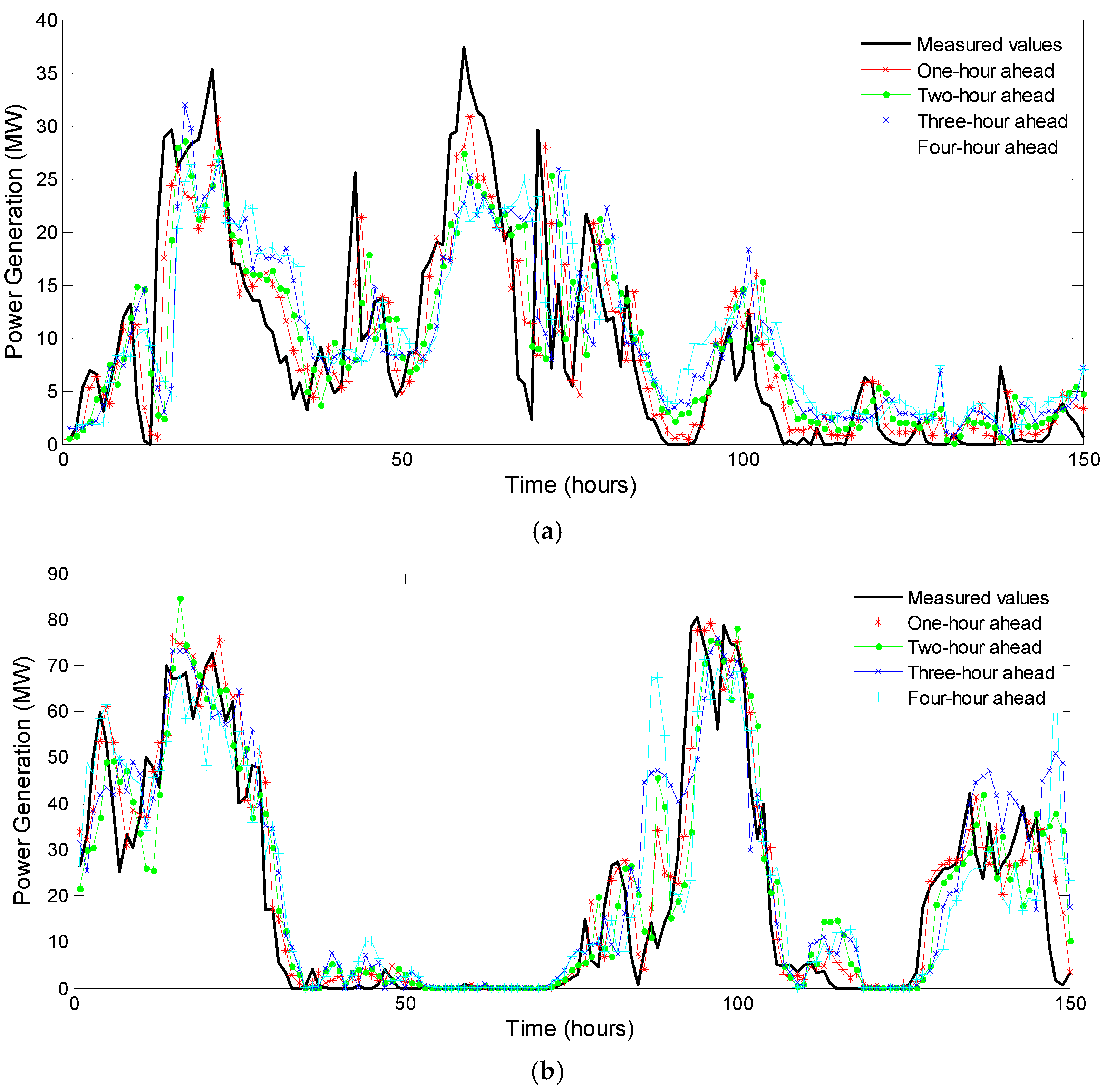
For different prediction steps, the corresponding selected samples are used to train the aforementioned hybrid prediction solution in Section 3. Here, the main parameters and settings for training the optimal ANFIS are summarized in

Table 3. Main setting parameters for training.

Main Techniques	Parameters and Settings
Hyperparameters of PSO	Inertia weight	$w_0=1$
	Inertia weight damping ratio	$w_{damp}=0.99$
	Individual learning coefficient	$c_1=1$
	Global learning coefficient	$c_2=2$
	Numbers of particles	$n_{pop}=30$
	Maximum number of iterations	$n_{ite}=100$
Hyperparameters of ANFIS	Number of fuzzy set in each input variable	$n_{fuzzy}=5$
Hyperparameters of K-means	Number of clustering centers	$k=6$
Number of samples in the two farms	Number of training samples	$n_{train}^{Az}=8832$$n_{train}^{Xq}=8736$
	Number of test samples	$n_{test}^{Az}=2880$$n_{test}^{Xq}=2796$

. After determining the ANFIS parameters by training samples, the multi-step ahead prediction results in the test month can be obtained. Figure 6 presents the prediction result of 150 h from the test month for two wind farms, respectively.

To evaluate the effectiveness and accuracy of the prediction solution, the performance metric in terms of normalized root mean squared error (nRMSE) and normalized mean absolute error (nMAE) are adopted [40], as given in Equations (27) and (28), respectively. In general, smaller values of these measures indicate that the corresponding solution has better prediction performance.

$$\mathrm{nRMSE}=\sqrt{\frac{1}{N}{{\displaystyle \sum _{i=1}^N\left(\frac{P_{mi}-P_{pi}}{C_i}\right)}}^2}$$

(27)

$$\mathrm{nMAE}=\frac{1}{N}{\displaystyle \sum _{i=1}^N\left|\frac{P_{mi}-P_{pi}}{C_i}\right|}$$

(28)

where $P_{pi}$ is the predicted power of time point $i$, $P_{mi}$ is the measured mean power of time point $i$, N is the number of prediction samples, and $C_i$ is the operating capacity of time point $i$.

To evaluate the proposed mRMR-criterion input variable selection (IVS) solution based prediction approach, mRMR-IVS model, a detailed comparative study was conducted for multi-step ahead wind power generation prediction. Two IVS based prediction approaches, the phase space reconstruction based (PSR-IVS) model and principal component analysis based (PCA-IVS) model, were selected as the comparative benchmark. For PSR-IVS based prediction model, the input variables included the NWP variables and the phase space reconstruction variables of the historical time series. The reconstruction was determined based on C_C method as well. In this model, the input variables were the ones which are candidates in proposed mRMR-IVS solution, without further exquisite selection. For PCA-IVS based model, the input variables were transformed from the combination of NWP variables and a time series of 2 h, which use the principal component analysis (PCA) technique [41] to map the dataset from the original space to the principal component space. In this model, the original attribute variables are automatically reduced to appropriate input variables and the independent principal components can well maintain the key characteristics of the original variables. After selecting or extracting the input variables, all the IVS-based approaches used the hybrid model introduced in Section 3 to carry out the predication.

Two error criteria, nRMSE and nMAE, were used to assess the performance of all considered prediction models.

Table 4. Comparison of the multi-step ahead prediction performance of Anzishan farm.

Prediction Time Steps	mRMR-IVS		PSR-IVS		PCA-IVS
	nRMSE (%)	nMAE (%)	nRMSE (%)	nMAE (%)	nRMSE (%)	nMAE (%)
#1	4.78	2.84	5.01	2.90	7.91	5.04
#2	6.67	4.10	6.74	4.27	9.25	5.98
#3	8.04	5.13	8.28	5.43	10.36	6.66
#4	9.64	6.12	10.01	6.64	10.98	7.43
#5	10.44	6.87	10.69	7.21	11.74	8.12
#6	11.18	7.43	11.31	7.96	13.03	8.93
#7	11.32	7.82	12.21	8.48	13.12	9.19
#8	12.02	8.38	13.19	8.81	14.97	10.15
#9	12.17	8.68	13.71	9.37	15.17	10.35
#10	12.54	8.99	13.37	9.64	14.11	9.80
#11	12.80	9.21	14.22	10.04	14.41	10.46
#12	12.88	9.36	15.02	10.66	14.50	10.30
#13	13.06	9.55	14.92	10.48	14.05	9.77
#14	13.17	9.65	14.69	10.49	14.89	10.69
#15	13.24	9.70	14.87	10.82	14.78	10.43
#16	13.51	9.97	14.60	10.39	15.27	10.88

and

Table 5. Comparison of the multi-step ahead prediction performance of Xuqiao farm.

Prediction Time Steps	mRMR-IVS		PSR-IVS		PCA-IVS
	nRMSE (%)	nMAE (%)	nRMSE (%)	nMAE (%)	nRMSE (%)	nMAE (%)
#1	4.04	2.34	4.06	2.35	8.19	4.98
#2	6.12	3.71	6.17	3.70	8.69	5.33
#3	7.39	4.47	7.81	4.91	9.72	6.02
#4	8.37	5.22	8.85	5.80	10.40	6.45
#5	9.86	6.28	9.89	6.50	11.53	7.10
#6	10.89	6.93	10.87	7.12	12.37	7.95
#7	11.55	7.34	11.62	7.45	12.65	8.41
#8	12.05	7.78	12.38	8.41	13.40	8.69
#9	12.50	8.02	12.86	8.68	13.66	8.81
#10	13.19	8.57	13.71	9.29	14.11	9.69
#11	13.55	8.85	13.62	9.34	14.82	9.72
#12	14.23	9.28	14.24	9.87	15.02	10.02
#13	14.27	9.39	15.23	10.69	15.69	10.53
#14	14.29	9.33	14.81	9.87	15.82	10.84
#15	14.54	9.68	15.21	10.41	15.79	10.72
#16	14.71	9.65	15.50	10.56	16.35	10.94

show the comparison of multi-step ahead prediction performance of different models for two wind farms, respectively. As shown in Table 4 and Table 5, the proposed model demonstrates the smallest error over all 16 steps of prediction compared with both benchmark models. In addition, compared with the principal component analysis-based model (PCA-IVS), the phase space reconstruction based (PSR-IVS) model performs better in short step prediction, but has larger error in long prediction period. Due to the sophisticated and targeted input variable selection, the proposed model has a better performance than the benchmark models in the overall multi-step ahead prediction.

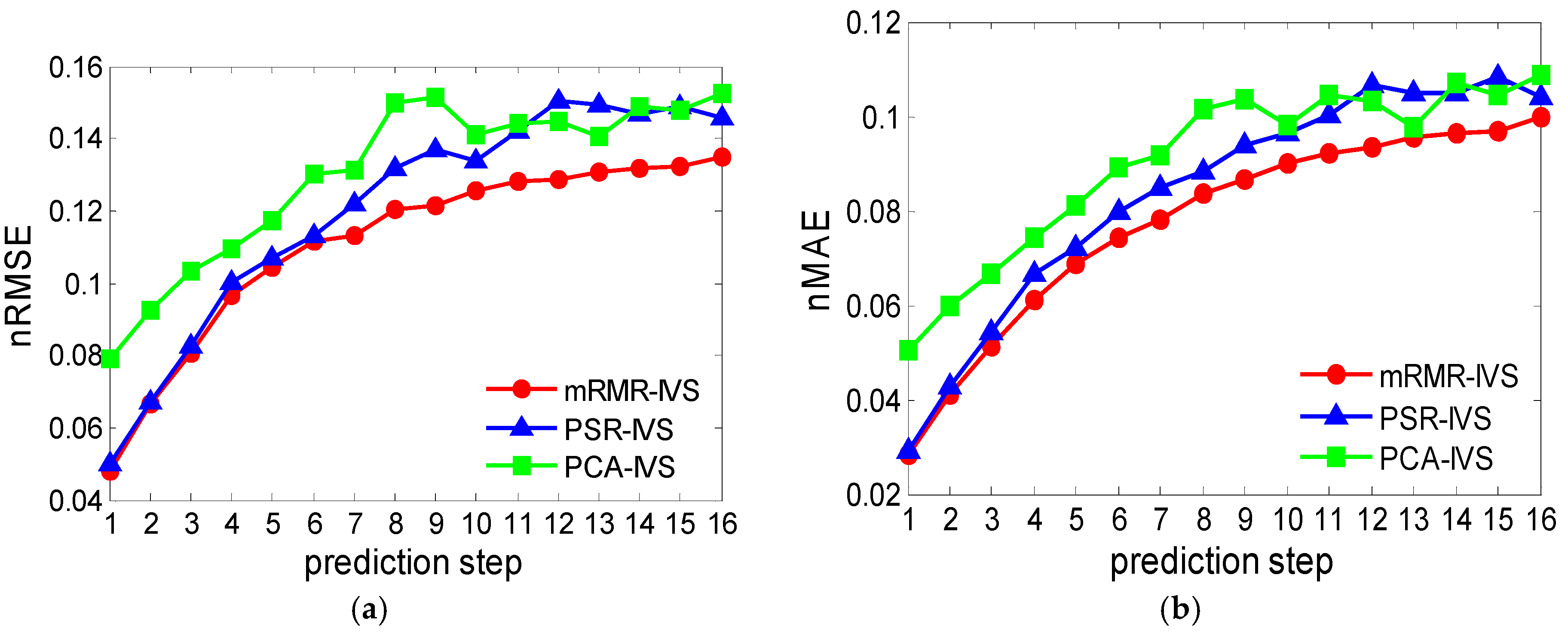
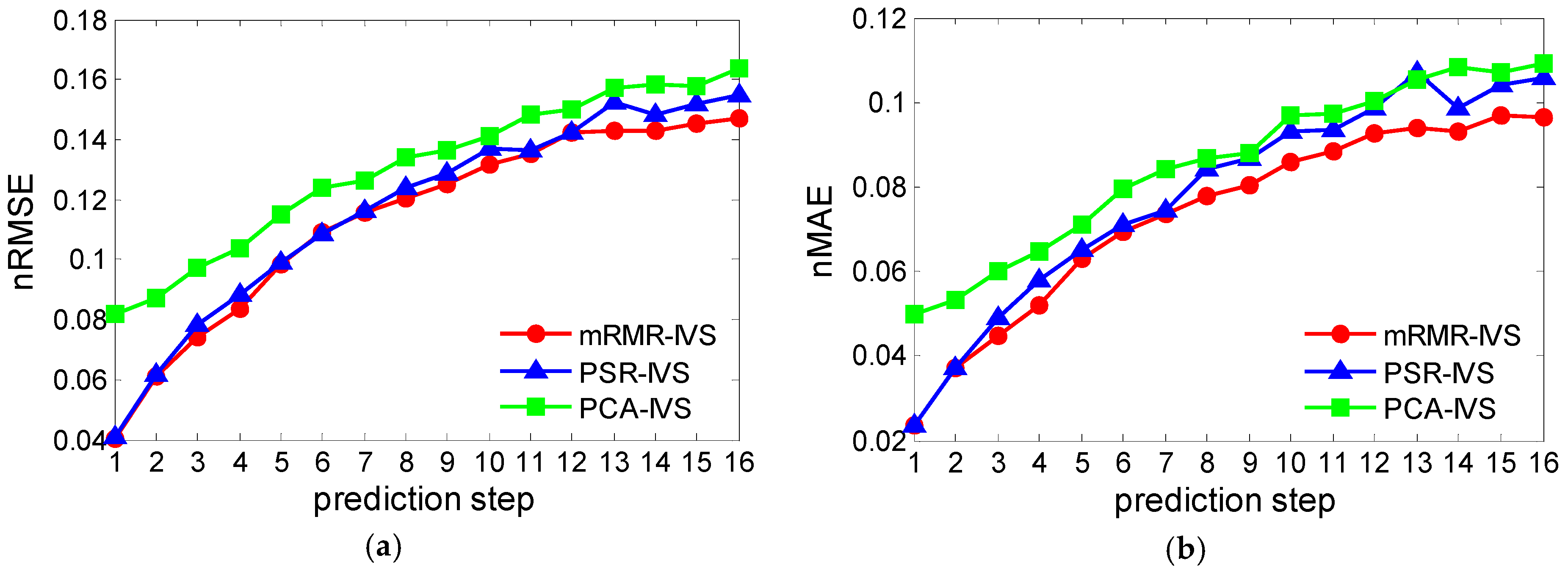
To present the comparison more intuitively, Figure 7 and Figure 8 show the broken line in two wind farms of three cases based on the values of nRMSE and nMAE of different prediction steps. The curve trend shows that the error level rises with the increase of prediction step, meeting the objective expectation. It is shown that there are fluctuations in the curve of two benchmark models, especially in the intermediate prediction period, in that the selection of input variables cannot adapt to each prediction step. In the proposed model, the error trend increased smoothly, indicating that the mRMR-IVS based model can automatically select the optimal or nearly optimal input variables for different prediction steps to reduce the error. It means that the proposed hybrid solution can select suitable input variables effectively in different geographical environments and seasons, showing better adaptability and robustness.

To further validate the integral time-scales of ultra-short-term wind power prediction, which is generally 0–4 h in the future with a resolution of 15 min, 100 integrated time series with consecutive 4-h prediction were randomly selected during the test-month forecasting process to calculate the performance metric in statistics. The nRMSE and nMAE indicators of each integrated time series were calculated. Then, the probability of different error levels could be obtained according to the statistics of appearing frequency in these 100 results. The average errors and the probability distribution of typical error levels of Anzishan and Xuqiao wind farms are shown in

Table 6. Mean errors and probability distributions of Anzishan farm.

Models	Mean nRMSE	Error Level for$\mathbf{P}\left\{\mathbf{n}\mathbf{R}\mathbf{M}\mathbf{S}\mathbf{E}<0.2\right\}$	Error Level for$\mathbf{P}\left\{\mathbf{n}\mathbf{R}\mathbf{M}\mathbf{S}\mathbf{E}<0.15\right\}$	Error Level for$\mathbf{P}\left\{\mathbf{n}\mathbf{R}\mathbf{M}\mathbf{S}\mathbf{E}<0.05\right\}$
mRMR-IVS	9.95%	93.80%	82.40%	16.8%
PSR-IVS	10.75%	89.80%	82.40%	10.90%
PCA-IVS	11.79%	88.20%	76.10%	9.80%
Models	Mean nMAE	Error Level for$\mathbf{P}\left\{\mathbf{n}\mathbf{M}\mathbf{A}\mathbf{E}<0.2\right\}$	Error Level for$\mathbf{P}\left\{\mathbf{n}\mathbf{M}\mathbf{A}\mathbf{E}<0.15\right\}$	Error Level for$\mathbf{P}\left\{\mathbf{n}\mathbf{M}\mathbf{A}\mathbf{E}<0.05\right\}$
mRMR-IVS	7.84%	98.20%	92.80%	32.10%
PSR-IVS	8.88%	94.00%	87.40%	21.20%
PCA-IVS	9.65%	93.30%	84.90%	18.10%

and

Table 7. Mean errors and probability distributions of Xuqiao farm.

Models	Mean nRMSE	Error Level for$\mathbf{P}\left\{\mathbf{n}\mathbf{R}\mathbf{M}\mathbf{S}\mathbf{E}<0.2\right\}$	Error Level for$\mathbf{P}\left\{\mathbf{n}\mathbf{R}\mathbf{M}\mathbf{S}\mathbf{E}<0.15\right\}$	Error Level for$\mathbf{P}\left\{\mathbf{n}\mathbf{R}\mathbf{M}\mathbf{S}\mathbf{E}<0.05\right\}$
mRMR-IVS	9.71%	91.60%	80.80%	27.00%
PSR-IVS	10.41%	90.00%	75.30%	26.60%
PCA-IVS	11.47%	84.00%	69.60%	25.30%
Models	Mean nMAE	Error Level for$\mathbf{P}\left\{\mathbf{n}\mathbf{M}\mathbf{A}\mathbf{E}<0.2\right\}$	Error Level for$\mathbf{P}\left\{\mathbf{n}\mathbf{M}\mathbf{A}\mathbf{E}<0.15\right\}$	Error Level for$\mathbf{P}\left\{\mathbf{n}\mathbf{M}\mathbf{A}\mathbf{E}<0.05\right\}$
mRMR-IVS	7.62%	96.80%	89.10%	38.40%
PSR-IVS	8.70%	94.00%	84.00%	32.30%
PCA-IVS	9.73%	89.80%	77.40%	31.50%

, respectively. For both cases, the proposed mRMR-IVS based solution demonstrates the minimum mean errors. The results given in Table 6 and Table 7 verify that the proposed model is more competitive for most probability distributions at different error levels. This clearly confirms that the proposed solution can provide improved prediction performance than the comparison benchmarks.

5. Conclusions and Future Work

This paper develops a novel algorithmic solution for ultra-short-term wind power generation prediction using hybrid machine learning techniques. The proposed solution is implemented through two steps: firstly, the input variable selection (IVS) is carried out using phase space reconstruction (PSR) technique and minimal redundancy maximal relevance (mRMR) criterion. Secondly, the input instances are divided into a set of subsets using the K-means clustering to train the ANFIS with parameters optimized using PSO. The proposed solution was extensively evaluated and validated through case studies based on real wind farms. The numerical results demonstrate the superiority of the proposed model compared with the benchmark models.

In the future, two research directions are considered worth further research effort. The proposed prediction solution can be further exploited using other supervised learning algorithms and advanced error correction techniques as well as extensively validated based on more field measurements. The hybrid machine learning techniques can be further extended and incorporated into control and management strategies of renewable energy systems (e.g., [42,43,44,45]) to improve the system operational performance.

References

- Ponta, L.; Raberto, M.; Teglio, A.; Cincotti, S. An agent-based stock-flow consistent model of the sustainable transition in the energy sector. Ecol. Econ. 2018, 145, 274–300. [Google Scholar] [CrossRef]
- Filippo, A.D.; Lombardi, M.; Milano, M. User-aware electricity price optimization for the competitive market. Energies 2017, 10, 1378. [Google Scholar] [CrossRef]
- Huang, C.M.; Kuo, C.J.; Huang, Y.C. Short-term wind power forecasting and uncertainty analysis using a hybrid intelligent method. IET Renew. Power Gen. 2017, 11, 678–687. [Google Scholar] [CrossRef]
- Weron, R. Electricity price forecasting: a review of the state-of-the-art with a look into the future. Int. J. 2014, 30, 1030–1081. [Google Scholar] [CrossRef]
- Cincotti, S.; Gallo, G.; Ponta, L.; Raberto, M. Modeling and forecasting of electricity spot-prices: computational intelligence vs classical econometrics. Ai Commun. 2014, 27, 301–314. [Google Scholar]
- Giebel, G.; Brownsword, R.; Kariniotakis, G. The State-Of-The-Art in Short-Term Prediction of Wind Power: A Literature Overview; Technical Report for ANEMOS.plus: Roskilde, Denmark, 2011. [Google Scholar]
- Costa, A.; Crespo, A.; Navarro, J.; Lizcano, G.; Madsen, H.; Feitosa, E. A review on the young history of the wind power short-term prediction. Renew. Sustain. Energy Rev. 2008, 12, 1725–1744. [Google Scholar] [CrossRef] [Green Version]
- Li, G.; Shi, J. On comparing three artificial neural networks for wind speed forecasting. Appl. Energy 2010, 87, 2313–2320. [Google Scholar] [CrossRef]
- Zhou, J.; Shi, J.; Li, G. Fine tuning support vector machines for short-term wind speed forecasting. Energy Convers. Manag. 2011, 52, 1990–1998. [Google Scholar] [CrossRef]
- Taslimi Renani, E.; Elias, M.F.M.; Rahim, N.A. Using data-driven approach for wind power prediction: A comparative study. Energy Convers. Manag. 2016, 118, 193–203. [Google Scholar] [CrossRef]
- Lee, D.; Baldick, R. Short-term wind power ensemble prediction based on gaussian processes and neural networks. IEEE Trans. Smart Grid 2014, 5, 501–510. [Google Scholar] [CrossRef]
- Guo, Z.; Chi, D.; Wu, J.; Zhang, W. A new wind speed forecasting strategy based on the chaotic time series modelling technique and the apriori algorithm. Energy Convers. Manag. 2014, 84, 140–151. [Google Scholar] [CrossRef]
- Xue, Y.; Yu, C.; Li, K.; Wen, F.; Ding, Y.; Wu, Q. Adaptive ultra-short-term wind power prediction based on risk assessment. Csee J. Power Energy Syst. 2016, 2, 59–64. [Google Scholar] [CrossRef]
- Safari, N.; Chung, C.Y.; Price, G.C.D. A novel multi-step short-term wind power prediction framework based on chaotic time series analysis and singular spectrum analysis. IEEE Trans. Power Syst. 2017, 99, 590–601. [Google Scholar] [CrossRef]
- Santamaría-Bonfil, G.; Reyes-Ballesteros, A.; Gershenson, C. Wind speed forecasting for wind farms: A method based on support vector regression. Renew. Energy 2016, 85, 790–809. [Google Scholar] [CrossRef]
- Buhan, S.; Cadirci, I. Multistage wind-electric power forecast by using a combination of advanced statistical methods. IEEE Trans. Ind. Inform. 2015, 11, 1231–1242. [Google Scholar] [CrossRef]
- Fang, S.; Chiang, H.D. A high-accuracy wind power forecasting model. IEEE Trans. Power Syst. 2017, 32, 1589–1590. [Google Scholar] [CrossRef]
- Fang, S.; Chiang, H.D. Improving supervised wind power forecasting models using extended numerical weather variables and unlabelled data. IET Renew. Power Gen. 2016, 10, 1616–1624. [Google Scholar] [CrossRef]
- Fu, T. A review on time series data mining. Appl. Artif. Intell. 2011, 24, 164–181. [Google Scholar] [CrossRef]
- Zhao, X.; Deng, W.; Shi, Y. Feature selection with attributes clustering by maximal information coefficient. Procedia Comput. Sci. 2013, 17, 70–79. [Google Scholar] [CrossRef]
- Zhao, H.; Magoulès, F. Feature selection for predicting building energy consumption based on statistical learning method. J. Algorithms Comput. Technol. 2012, 6, 59–78. [Google Scholar] [CrossRef]
- Kapetanakis, D.-S.; Mangina, E.; Finn, D.P. Input variable selection for thermal load predictive models of commercial buildings. Energy Build. 2017, 137, 13–26. [Google Scholar] [CrossRef]
- Sharma, A.; Paliwal, K.K.; Imoto, S.; Miyano, S. A feature selection method using improved regularized linear discriminant analysis. Mach. Vis. Appl. 2013, 25, 775–786. [Google Scholar] [CrossRef] [Green Version]
- Zjavka, L.; Misak, S. Direct wind power forecasting using a polynomial decomposition of the general differential equation. IEEE Trans. Sustain. Energy 2018, 99. [Google Scholar] [CrossRef]
- Takens, F. Detecting strange attractors in turbulence. Lecture Notes in Mathematics-Springer-verlag-(Lect Notes Math). In Lecture Notes Math; Rand, D.A., Young, L.-S., Eds.; Springer: Berlin, Germany, 1981; Volume 898, pp. 366–381. [Google Scholar]
- Kim, H.S.; Eykholt, R.; Salas, J.D. Nonlinear dynamics, delay times, and embedding windows. Phys. D Nonlinear Phenom. 1999, 127, 48–60. [Google Scholar] [CrossRef]
- Niu, T.; Wang, J.; Lu, H.; Du, P. Uncertainty modeling for chaotic time series based on optimal multi-input multi-output architecture: Application to offshore wind speed. Energy Convers. Manag. 2018, 156, 597–617. [Google Scholar] [CrossRef]
- Maji, P.; Garai, P. On fuzzy-rough attribute selection: criteria of max-dependency, max-relevance, min-redundancy, and max-significance. Appl. Soft Comput. 2013, 13, 3968–3980. [Google Scholar] [CrossRef]
- Wang, X.; Han, M.; Wang, J. Applying input variables selection technique on input weighted support vector machine modeling for bof endpoint prediction. Appl. Artif. Intell. 2010, 23, 1012–1018. [Google Scholar] [CrossRef]
- Battiti, R. Using mutual information for selecting features in supervised neural net learning. IEEE Trans. Neural Netw. 1994, 5, 537–550. [Google Scholar] [CrossRef] [PubMed] [Green Version]
- Kwak, N.; Choi, C.-H. Input feature selection by mutual information based on Parzen window. IEEE Trans. Pattern Anal. Mach. Intell. 2002, 24, 1667–1671. [Google Scholar] [CrossRef]
- Estevez, P.A.; Tesmer, M.; Perez, C.A.; Zurada, J.M. Normalized mutual information feature selection. IEEE Trans. Neural Netw. 2009, 20, 189–201. [Google Scholar] [CrossRef] [PubMed]
- Cover, T.; Thomas, J. Elements of Information Theory; Wiley-Blackwell: Hoboken, NJ, USA, 2006. [Google Scholar]
- Ponta, L.; Carbone, A. Information measure for financial time series: quantifying short-term market heterogeneity. Phys. A Stat. Mech. Appl. 2018, 510, 123–144. [Google Scholar] [CrossRef]
- Bandt, C.; Pompe, B. Permutation entropy: a natural complexity measure for time series. Phys. Rev. Lett. 2002, 88. [Google Scholar] [CrossRef] [PubMed]
- Celebi, M.E.; Kingravi, H.A.; Vela, P.A. A comparative study of efficient initialization methods for the k-means clustering algorithm. Expert Syst. Appl. 2013, 40, 200–210. [Google Scholar] [CrossRef] [Green Version]
- Jang, J.-S.R. Anfis: Adaptive-network-based fuzzy inference system. IEEE Trans. Syst. Man. Cybern. 1993, 23, 665–685. [Google Scholar] [CrossRef]
- Ghosh, S.; Kumar, S. Comparative analysis of k-means and fuzzy c-means algorithms. Int. J. Adv. Comput. Sci. Appl. 2013, 4. [Google Scholar] [CrossRef]
- Kennedy, J.; Eberhart, R.C. Particle swarm optimization. In Proceedings of the IEEE International Conference on Neural Networks, Perth, WA, Australia, 27 November–1 December 1995; pp. 1942–1948. [Google Scholar]
- Madsen, H.; Pinson, P.; Kariniotakis, G.; Nielsen, H.A.; Nielsen, T.S. Standardazing the performance evaluation of short term wind power prediction models. Wind Eng. 2005, 29, 475–489. [Google Scholar] [CrossRef] [Green Version]
- Wu, Q.; Peng, C. Wind power generation forecasting using least squares support vector machine combined with ensemble empirical mode decomposition, principal component analysis and a bat algorithm. Energies 2016, 9, 261. [Google Scholar] [CrossRef]
- Baghaee, H.R.; Mirsalim, M.; Gharehpetian, G.B.; Talebi, H.A. Three-phase ac/dc power-flow for balanced/unbalanced microgrids including wind/solar, droop-controlled and electronically-coupled distributed energy resources using radial basis function neural networks. IET Power Electron. 2017, 10, 313–328. [Google Scholar] [CrossRef]
- Baghaee, H.R.; Mirsalim, M.; Gharehpetian, G.B. Power Calculation Using RBF Neural Networks to Improve Power Sharing of Hierarchical Control Scheme in Multi-DER Microgrids. IEEE J. Emerg. Sel. Top. Power Electron. 2016, 4, 1217–1225. [Google Scholar] [CrossRef]
- Baghaee, H.R.; Mirsalim, M.; Gharehpetan, G.B.; Talebi, H.A. Nonlinear load sharing and voltage compensation of microgrids based on harmonic power-flow calculations using radial basis function neural networks. IEEE Syst. J. 2016, PP, 1–11. [Google Scholar] [CrossRef]
- Morshed, M.J.; Hmida, J.B.; Fekih, A. A probabilistic multi-objective approach for power flow optimization in hybrid wind-pv-pev systems. Appl. Energy 2018, 211, 1136–1149. [Google Scholar] [CrossRef]
Figure 1.
The framework of the proposed hybrid algorithmic solution.
Figure 2.
Typical two-input ANFIS structure.
Figure 3.
Results of and produced by the C_C method in Anzishan farm.
Figure 4.
Results of and produced by the C_C method in Xuqiao farm.
Figure 5.
Cumulative informativeness score curve for IVS of Anzishan and Xuqiao farms: (a) one-hour ahead prediction; (b) two-hour ahead prediction; (c) three-hour ahead prediction; and (d) four-hour ahead prediction.
Figure 6.
Partial results of multi-step ahead prediction in the test month: (a) power generation prediction of 150 h in Anzishan wind farm (June 2017); and (b) power generation prediction of 150 h in Xuqiao wind farm (December 2017).
Figure 7.
Error trend in different prediction steps of Anzishan farm: (a) nRMSE of test month; and (b) nMAE of test month.
Figure 8.
Error trend in different prediction steps of Xuqiao farm: (a) nRMSE of test month; and (b) nMAE of test month.