A New Lumped Parameter Model for Natural Gas Pipelines in State Space

Abstract

Many algorithms and numerical methods, such as implicit and explicit finite differences and the method of characteristics, have been applied for transient flow in gas pipelines. From a computational point of view, the state space model is an effective method for solving complex transient problems in pipelines. However, the impulse output of the existing models is not the actual behavior of the pipeline. In this paper, a new lumped parameter model is proposed to describe the inertial nature of pipelines with inlet/outlet pressure and flow rate as outer variables in the state space. Starting from the basic mechanistic partial differential equations of the general one-dimensional compressible gas flow dynamics under isothermal conditions, the transfer functions are first acquired as the fundamental work. With Taylor-expansion and a transformation procedure, the inertia state space models are derived with proper simplification. Finally, three examples are used to illustrate the effectiveness of the proposed model. With the model, a real-time automatic scheduling scheme of the natural gas pipeline could be possible in the future.

1. Introduction

The consumption of natural gas is growing rapidly due to its environmentally-friendly characteristics and low price. From field-processing facilities, dried and cleaned natural gas enters the gas transmission pipeline system to cities where it is distributed to individual businesses, factories, and residences. The transportation of natural gas over a large geographic area requires efficient operation of the compressors and other related facilities. The scheduling of a piping system is a great challenge to control theory.

Current industrial practice for long distance natural gas pipeline control involve regulatory control loops along with manual intervention by pipeline operators. Operators must calculate the transportability of the required gas quantity and determine the production set-point of each compressor plant and the valve. The transportation planning process based on specified requirements is influenced by various factors, including the current state of the transmission system, maintenance requirements, gas storage availability, line pack, shippers contracts, etc. The operation commands work on SCADA systems [1]. SCADA stands for Supervisory Control And Data Acquisition and is a standard configuration in modern pipeline systems.

With the help of SCADA systems, the real-time data from field is collected and can be used for system identification [2]. There some empirical parameters, such as the efficiency coefficient for pipeline sections, the technical state coefficients for compressors, and other parameters that characterize the valves. Considering the identification problem for the parameters, coefficient estimation is reduced to an optimization problem. Meanwhile, since the main problems in the data are the noisy and imprecise sensors used only at the end of the pipelines, conventional state estimation can be implemented by actually solving identification models [3]. By treating some subset of the measurements as constraints, the model results in all of the pressure and flow meters, which is described in more detail in reference [4].

The SCADA system is the control center of the natural gas pipeline, but is currently focused at the supervisory level. Compared with the advances in the hardware configuration of pipelines, the scheduling scheme is still an empirical decision process. Due to the lack of an effective mathematical model for the pipeline, it is impossible to implement the control scheme automatically [5].

As an airtight transmitting system with high pressure, the dynamic behavior of long distance pipelines is characterized by large time constants due to the resistance to flow in pipes and the large storage capacity of the pipelines [6]. The governing equations for such complex and large-scale systems consist of a set of nonlinear hyperbolic partial differential equations. The PDEs (partial differential equations) describe the behavior of gas flow in pipelines in complex ways and can only be solved numerically. The method of characteristics, explicit and implicit finite difference methods, and finite element methods have been used to solve the governing equations to obtain good simulation results [7]. These studies aim to simulate the unsteady flow in a pipeline accurately. For large systems with hundreds or even thousands of interconnected pipeline elements, the solution process needs plenty of computing time and storage. Thus, real-time simulation of gas pipelines and networks is not possible with PDEs.

Because of the limitations of simulation methods, there is no efficient way to plan transmission. The operating schemes for the pipelines in the face of varying demand are established by a trial and error method in the simulation platform. A control-oriented mathematical model and the corresponding algorithm are necessary for automated scheduling processes. The challenges are the system’s large dimensions, nonlinearity, and the operational constraints. In addition, the internal states of the system are usually unknown due to the limited number of measurements. The body of literature on gas pipeline control is rather rare. Sanada and Kitagawa [8] formulated a linear $H_1$ controller for a very simple gas pipeline described by ordinary differential equations that were obtained by the discretization of a PDE model [9].

Recently, state space models were used for transient flow simulation in gas pipelines and networks by Alamian et al. [10]. Prior to their work, some S-functions were developed to simulate transient flow in gas pipeline networks in MATLAB-Simulink [11,12]. Also, transfer function models were proposed as an efficient transient flow simulation method for gas pipelines and networks [13]. There are some other reduced order models described in reference [14]. The modeling methods always involve the following steps:

• The equivalent transfer functions are derived from the governing equations;
• The series form of the models in the time domain is obtained using the convolution theorem;
• A few dominant flow eigenmodes are used to construct an efficient reduced-order model, i.e., ODE (ordinary differential equation) model.

As seen from the above, the state space models neglect some of the terms in PDEs and maintain an appropriate level of accuracy at the same time. Due to the convenience of the state space model, it can be easily applied for large and complicated network controller designs by following the control theory. The ODE models are more useful in controller design because of their similarity to pipeline input/output dynamics.

There is a problem for existing ODE models, whereby the fast responses of ODEs are not appropriate for the natural gas pipeline. The time scale between the input end variation and the output end reaction is usually measured in hours. Matrix $\mathbb{D}$ in state space models like Equation (31) is the feed-forward matrix. It is a direct channel through which the input signal can affect the output signal immediately. Thus, a large amplitude and high frequency input signal results in corresponding variation of the output’s end behavior. Matrix $\mathbb{D}$ leads to the impulse response of pressure or flow in the existing models. The sudden change in process parameters does not happen in real piping. The model characteristics deviate from the actual phenomenon of the pipeline. So, the objective of this paper is to develop a state space model with greater accuracy and no direct channel between the input and the output.

The rest of the paper is organized as follows. In Section 2, the mechanism of the transient flow in a gas pipeline is described. Then, a simplified model is proposed, and the flow transfer functions are derived. In Section 3, the state space model for different boundary conditions are derived based on the transfer functions. In Section 4, different examples are used to analyze and simulate the transient behaviors of a gas pipeline and a network. The results are compared with the commercial software SPS (Stoner Pipeline Simulator) and the models given in reference [10].

2. Mathematical Models

2.1. Mechanism Model

The gas flow through pipelines is generally governed by the conservation mass, momentum, energy, and a state equation, which are used to obtain the pressure, velocity, density, and temperature. For infinitesimal control volume of a general one-dimensional gas flow through a constant diameter and rigid pipeline, these hyperbolic partial differential equations are

$$\frac{\partial \rho }{\partial t}+\frac{\partial \left(\rho u\right)}{\partial x}=0,$$

(1)

$$\frac{\partial p}{\partial x}=-\frac{\partial \left(\rho u\right)}{\partial t}-\lambda \frac{u\left|u\right|}{2D}\rho -\rho g\sin \alpha ,$$

(2)

$$\frac{\partial Q}{\partial x}(\rho u)=\frac{\partial }{\partial t}[(\rho )(\widehat{u}+\frac{u^2}{2}+g\Delta h)]+\frac{\partial }{\partial x}[(\rho )(H+\frac{u^2}{2}+gs)],$$

(3)

$$\frac{p}{\rho }=ZRT,$$

(4)

where $\rho$ is the gas density in kg/m${}^3$; D is the pipeline inner diameter in m; g is the gravitational acceleration in m/s${}^2$; $\alpha$ is the inclination; R is the gas constant in kJ/(kg·K); $\lambda$ is the friction factor of the pipeline; Z is the gas compressibility factor; u is the gas axial velocity in m/s; T is the gas temperature in K; $\frac{\partial Q}{\partial x}$ is the heat flow into the pipe per unit length of pipe and per unit time in J/(m·s); $\widehat{u}$ is the specific internal energy in J/kg; $\Delta h$ is the elevation in m; H is the specific enthalpy in J/kg; x is pipeline coordinate in m; and t is the time in s.

For the quadratic resistance region (typical flow condition in gas pipelines), the friction factor is generally described by the empirical Coolebrook–White correlation which can only be solved iteratively. The equations are an approximation of HOFER which is reasonable for the quadratic resistance region in gas pipelines. The gas compressibility factor relates the pressure, density, and temperature for the given components and can be approximated by the following equation which is valid for natural gas [15]:

$$\lambda =[2{log}_{10}(\frac{4.518}{\mathrm{Re}}{log}_{10}(\frac{\mathrm{Re}}{7})+\frac{r}{3.71D}){]}^{-2},$$

(5)

$$Z=1+ap-\frac{bp}{T}=\frac{1}{1+\rho (b^{\ast }-a^{\ast }T)},$$

(6)

$$a=0.257/p_c,$$

(7)

$$b=0.533T_c/p_c,$$

(8)

$$a^{\ast }=aR,$$

(9)

$$b^{\ast }=bR,$$

(10)

where Re is the Reynold’s number of the gas; r is the pipeline roughness in m; $p_c$ is the critical pressure of the gas in Pa; and $T_c$ is the critical temperature of the gas in K.

Due to the degradation of steel pipes, compressors and so on, the technical state of a gas pipeline system deteriorates. The introduced empirical parameters in the models account for these changes. The system’s PDE model is adapted by identifying these coefficients by gauging the operating parameters of the gas flow, pressure, and flow rate [2].

The governing equations for a transient subsonic flow analysis of natural gas in pipelines are a set of nonlinear hyperbolic partial differential equations. Many algorithms and numerical methods, such as implicit and explicit finite differences, the method of characteristics, etc., have been applied for transient flow analyses in gas pipelines [7]. These methods are well studied and integrated into commercial softwares such as SPS. These kinds of software are widely used in practice. In addition, SPS is used in Section 4 as a benchmark for the comparison of different models.

2.2. Transfer Function Model

In this section, the most common assumptions that have been thoroughly discussed in the literature are used to simplify the PDEs.

• The variation in gas temperature is negligible. The gas temperature is assumed to beconstant in space and time and is equal to the ground temperature;
• The influence of the convective term is negligible in the momentum equation because of the typically small flow velocities in gas transport pipelines (u ≤ 15 m/s).

The equations are solved based on the available flow rate, pressure, and density measurements which are sampled at regular time intervals. Since the volume flow rate requires compensation related to the pressure and temperature while the mass flow rate does not, the mass flow rate is used as a reference for the gas velocity in the following calculation. In addition, the simplified model, shown in Equations (11) and (12), representing the transient behaviors of the gas flow is derived from Equations (1)–(5) [10].

$$\frac{\partial \left(\frac{p}{ZRT}\right)}{\partial t}+\frac{1}{A}\frac{\partial m}{\partial x}=0,$$

(11)

$$\frac{\partial p}{\partial x}=-\frac{1}{A}\frac{\partial m}{\partial t}-\lambda \frac{m\left|m\right|}{2D{A}^{2}p}ZRT-g\frac{\Delta h}{L}\frac{p}{ZRT},$$

(12)

where A is the cross-sectional area of the pipeline in m${}^2$; m is the gas mass flow rate in kg/s; and L is the length of the pipeline in m.

In piping systems, the system is in a steady-state if the process variables, such as pressure and flow rate, which define the behavior of the system are unchanging in time. The steady-state parameters are obtained by some simple calculation of the hydraulic equations. Here, steady-state corresponds to the transient state. A piping system is said to be in a transient state when process variables, such as pressure and flow rate, change and the system has not yet reached a steady-state. To obtain the transfer functions, the PDEs of Equations (11) and (12) are linearized with respect to the steady-state of the given boundary conditions. The results in the following linear PDEs are similar to those obtained in reference [10].

$$\frac{\partial \Delta m(\xi ,t)}{\partial \xi }+\frac{AL}{{\tilde{c}}^2}\frac{\partial \Delta p(\xi ,t)}{\partial t}=0,$$

(13)

$$\frac{\partial \Delta p(\xi ,t)}{\partial \xi }+L(gsin\theta )\frac{\Delta p(\xi ,t)}{{\tilde{c}}^2}-\frac{\lambda L\tilde{w}\left|\tilde{w}\right|}{2D{\tilde{c}}^2}\Delta p(\xi ,t)+\frac{\lambda L\tilde{w}}{DA}\Delta m(\xi ,t)+\frac{L}{A}\frac{\partial \Delta m(\xi ,t)}{\partial t}=0,$$

(14)

where

$$\begin{array}{c}\Delta m\left(x,t\right)=m(x,t)-m(x,0),\hfill \\ \Delta p\left(x,t\right)=p(x,t)-p(x,0),\hfill \\ \xi =\frac{x}{L},\hfill \\ {\tilde{c}}^2=ZRT,\hfill \\ \tilde{w}=\frac{m(x,0){\tilde{c}}^2}{A\tilde{p}(x,0).}\hfill \end{array}$$

(15)

By Laplace transformation, we obtain the following two coupled linear ODEs with mathematical treatments [16]:

$$\frac{\partial \Delta m(\xi ,s)}{\partial \xi }+\frac{AL}{{\tilde{c}}^2}s\Delta p(\xi ,s)=0,$$

(16)

$$\frac{\partial \Delta p(\xi ,s)}{\partial \xi }+L(gsin\theta )\frac{\Delta p(\xi ,s)}{{\tilde{c}}^2}-\frac{\lambda L\tilde{w}\left|\tilde{w}\right|}{2D{\tilde{c}}^2}\Delta p(\xi ,s)+\frac{\lambda L\tilde{w}}{DA}\Delta m(\xi ,s)+\frac{L}{A}s\Delta m(\xi ,s)=0.$$

(17)

Equations (16) and (17) can now be written in matrix form as

$$\left[\begin{array}{c}\frac{\partial \Delta p(\xi ,s)}{\partial \xi }\hfill \\ \frac{\partial \Delta m(\xi ,s)}{\partial \xi }\hfill \end{array}\right]=\left[\begin{array}{cc}\gamma & -\alpha \\ -\beta & 0\end{array}\right]\left[\begin{array}{c}\Delta p(\xi ,s)\hfill \\ \Delta m(\xi ,s)\hfill \end{array}\right],$$

(18)

where

$$\begin{array}{l}\gamma =-\frac{L(gsin\theta )}{{\tilde{c}}^2}+\frac{\lambda L\tilde{w}\left|\tilde{w}\right|}{2D{\tilde{c}}^2}\hfill \\ \alpha =\frac{\lambda L\tilde{w}}{DA}+\frac{L}{A}s\hfill \\ \beta =\frac{AL}{{\tilde{c}}^2}s.\hfill \end{array}$$

(19)

Equation (18) can be solved analytically to impose the boundary conditions in the Laplace domain. For natural gas pipelines, the boundary conditions are usually specified as the gas pressure at a pipeline’s inlet and outlet as well as the mass flow rate at the pipeline’s inlet and outlet. For example, if the pressure at the inlet and the mass flow rate at the outlet are specified as functions of time, we can solve the ODEs in the Laplace domain with

$$\Delta p_{out}(s)=e^{\frac{\gamma }{2}}\frac{2b}{2bcoshb-\gamma sinhb}\Delta p_{in}(s)+\frac{-2\alpha sinhb}{2bcoshb-\gamma sinhb}\Delta m_{out}(s),$$

(20)

$$\Delta m_{in}(s)=\frac{2\beta sinhb}{2bcoshb-\gamma sinhb}\Delta p_{in}(s)+e^{-\frac{\gamma }{2}}\frac{2b}{2bcoshb-\gamma sinhb}\Delta m_{out}(s),$$

(21)

where

$$b=\frac{\sqrt[2]{{\gamma }^2+4\alpha \beta }}{2}.$$

(22)

It is impossible to obtain the analytical solutions in the time domain. Therefore, the simplified transfer functions of Equations (20) and (21) are approximated by Taylor expansion:

$$\begin{array}{c}\Delta p_{out}(s)=k_1\frac{1}{1+a_{1}s+a_2{s}^2}\Delta p_{in}(s)+k_2\frac{1+T_{21}s}{1+a_{1}s+a_2{s}^2}\Delta m_{out}(s),\hfill \end{array}$$

(23)

$$\begin{array}{c}\Delta m_{in}(s)=\frac{T_{11}s}{1+a_{1}s+a_2{s}^2}\Delta p_{in}(s)+\frac{1}{1+a_{1}s+a_2{s}^2}\Delta m_{out}(s),\hfill \end{array}$$

(24)

where

$$k_1=e^{\gamma },$$

(25)

$$k_2=e^{\frac{\gamma }{2}}·\frac{\lambda L|\tilde{w}|}{DA}(1+\frac{1}{24}{\gamma }^2+\frac{1}{1920}{\gamma }^4),$$

(26)

$$a_1=e^{\frac{\gamma }{2}}·\frac{\lambda L^2|\tilde{w}|}{2D{\tilde{c}}^2}(1-\frac{1}{6}\gamma +\frac{1}{24}{\gamma }^2-\frac{1}{240}{\gamma }^3),$$

(27)

$$a_2=e^{\frac{\gamma }{2}}·\left(\frac{\lambda L^2\left|\tilde{w}\right|}{24D{\tilde{c}}^2}\frac{\lambda L^2\left|\tilde{w}\right|}{D{\tilde{c}}^2}\left(1-\frac{1}{10}\gamma \right)+\frac{L^2}{{\tilde{c}}^2}(1-\frac{1}{6}\gamma +\frac{1}{24}{\gamma }^2-\frac{1}{240}{\gamma }^3)\right),$$

(28)

$$T_{11}=e^{\frac{\gamma }{2}}·\frac{AL}{{\tilde{c}}^2}(1+\frac{1}{24}{\gamma }^2+\frac{1}{1920}{\gamma }^4),$$

(29)

$$T_{21}=\frac{D}{\lambda |\tilde{w}|}+\frac{\lambda L^2\left|\tilde{w}\right|}{D{\tilde{c}}^2}(1+\frac{1}{40}{\gamma }^2)\frac{1}{1+\frac{1}{4}{\gamma }^2+\frac{1}{320}{\gamma }^4}.$$

(30)

There are, in total, four couples of transfer functions between the input flow/pressure and the output flow/presure. In the following examples, only the one in Equations (23) and (24) is used. The construction of the other three couples is similar to the process above with a different combination of the specified boundary conditions.

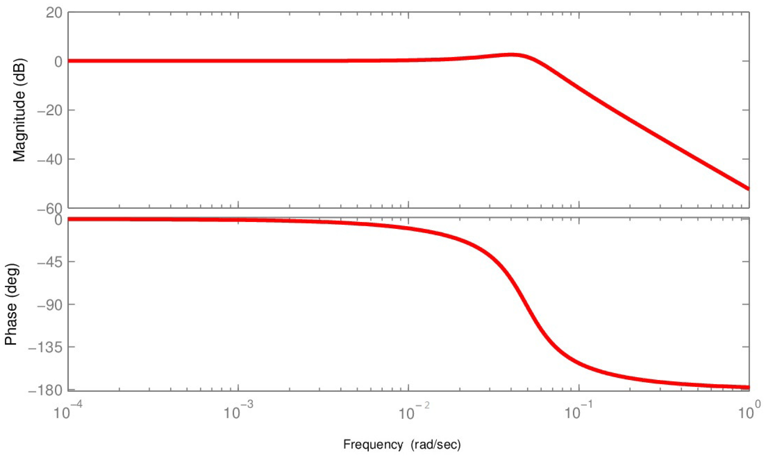
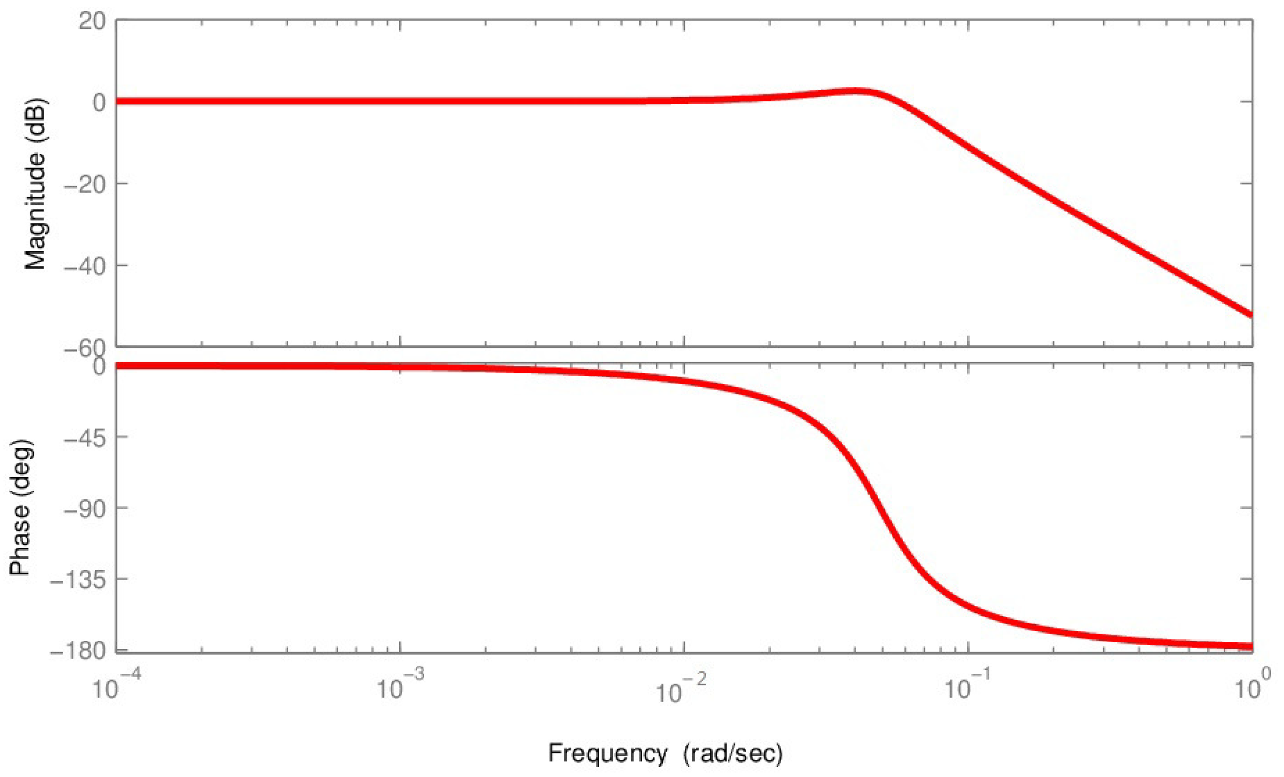
In order to see the input–output relationships, Bode plots of the system transfer functions are usually used to describe the steady-state response of the system. The following are the Bode plots of transfer function Equations (23) and (24) for a pipeline with $D=300$ mm and $L=\mathrm{10,000}$ m.

Remark 1.

From Figure 1 and Figure 2, one can see that the natural gas pipeline has a large time-delay and is a slow dynamic system. The system is like a low pass filter which has no response to input signals with high frequency. Based on this property, we eliminated matrix $\mathbb{D}$, which is totally different from the existing models. Since the models are derived from steady-state respect to given boundary conditions, their accuracy will be reduced if the steady-state changes. However, this shows the robustness to state deviations in a certain range in our following studies.

2.3. State Space Model

The transfer functions are used to derive the state space for transient analysis [14]. With different input/output couples, different state space models are derived. Equation (31) is the state space model with specified inputs, i.e., the gas pressure at inlet ($P_{in}$) and the mass flow rate at the outlet ($M_{out}$), and two outputs, i.e., the pressure at the outlet ($P_{out}$) and the gas mass flow rate at the inlet ($M_{in}$).

$$\begin{array}{c}\dot{x}=\mathbb{A}x+\mathbb{B}u,\hfill \\ y=\mathbb{C}x+\mathbb{D}u,\hfill \end{array}$$

(31)

where $u=[P_{in},M_{out}]$ and $y=[P_{out},M_{in}]$.

$$\begin{array}{c}\mathbb{A}=\left[\begin{array}{cccc}-\frac{a_1}{a{}_2}& 1& 0& 0\\ 0& -\frac{1}{a_2}& 0& 0\\ 0& 0& -\frac{a_1}{a{}_2}& 1\\ 0& 0& -\frac{1}{a_2}& 0\end{array}\right],\hfill \\ \mathbb{B}=\left[\begin{array}{cc}0& -\frac{k_2{T}_{21}}{a_2}\\ \frac{k_1}{a_2}& -\frac{k_2}{a{}_2}\\ \frac{T_{11}}{a_2}& 0\\ 0& \frac{1}{a_2}\end{array}\right],\hfill \\ \mathbb{C}=\left[\begin{array}{cccc}1& 0& 0& 0\\ 0& 0& 1& 0\end{array}\right].\hfill \end{array}$$

(32)

For known pipeline inlet and outlet pressures ($P_{in}$, $P_{out}$), the following state space model can be obtained by same method:

$$\begin{array}{c}\dot{x}=\mathbb{A}x+\mathbb{B}u,\hfill \\ y=\mathbb{C}x+\mathbb{D}u,\hfill \end{array}$$

(33)

where $u=[P_{in},P_{out}]$ and $y=[M_{in},M_{out}]$.

$$\mathbb{A}=\left[\begin{array}{cccc}-\frac{a_1+T_{21}}{a_2+T_{22}+a_1{T}_{21}}& 1& 0& 0\\ -\frac{1}{a_2+T_{22}+a_1{T}_{21}}& 0& 0& 0\\ 0& 0& -\frac{T_{21}}{T_{22}}& 1\\ 0& 0& -\frac{1}{T_{22}}& 0\end{array}\right],$$

(34)

$$\mathbb{B}=\left[\begin{array}{cc}\frac{T_{11}}{a{}_2+T_{22}+a_1{T}_{21}}& -\frac{a1}{k_{2}a{}_2+k_2{T}_{22}+k_2{a}_1{T}_{21}}\\ \frac{k_1}{k_{2}a{}_2+k_2{T}_{22}+k_2{a}_1{T}_{21}}& -\frac{1}{k_{2}a{}_2+k_2{T}_{22}+k_2{a}_1{T}_{21}}\\ 0& -\frac{T_{11}}{k_2{T}_{22}}\\ \frac{k_1}{k_2{T}_{22}}& -\frac{1}{k_2{T}_{22}}\end{array}\right],$$

(35)

$$\mathbb{C}=\left[\begin{array}{cccc}1& 0& 0& 0\\ 0& 0& 1& 0\end{array}\right],$$

(36)

and

$$T_{22}=\frac{1}{1+\frac{1}{24}{\gamma }^2+\frac{1}{1920}{\gamma }^4}\left(\frac{D}{\lambda |\tilde{w}|}\frac{\lambda L^2\left|\tilde{w}\right|}{6D{\tilde{c}}^2}(1+\frac{1}{40}{\gamma }^2)+\frac{\lambda L^2\left|\tilde{w}\right|}{120D{\tilde{c}}^2}\frac{\lambda L^2\left|\tilde{w}\right|}{D{\tilde{c}}^2}+\frac{L^2}{6{\tilde{c}}^2}(1+\frac{1}{40}{\gamma }^2)\right).$$

(37)

Equation (38) is the state space model for the known gas mass flow rate at inlet ($M_{in}$) and the pressure at the outlet ($P_{out}$).

$$\begin{array}{c}\dot{x}=\mathbb{A}x+\mathbb{B}u,\hfill \\ y=\mathbb{C}x+\mathbb{D}u,\hfill \end{array}$$

(38)

where $u=[M_{in},P_{out}]$ and $y=[M_{out},P_{in}]$.

$$\begin{array}{c}\mathbb{A}=\left[\begin{array}{cccc}-\frac{k_2{T}_{11}}{k_2{T}_{12}+k_2{T}_{21}{T}_{11}}& 1& 0& 0\\ -\frac{k_1}{k_2{T}_{12}+k_2{T}_{21}{T}_{11}}& 0& 0& 0\\ 0& 0& -\frac{k_1{k}_2{T}_{11}}{k_1{k}_2{T}_{12}+k_1{k}_2{T}_{21}{T}_{11}}& 1\\ 0& 0& -\frac{k_1}{k_2{T}_{12}+k_2{T}_{21}{T}_{11}}& 0\end{array}\right],\hfill \\ \mathbb{B}=\left[\begin{array}{cc}\frac{k_1{a}_1}{k_2{T}_{12}+k_2{T}_{21}{T}_{11}}& -\frac{T_{11}}{k_2{T}_{12}+k_2{T}_{21}{T}_{11}}\\ \frac{k_1}{k_2{T}_{12}+k_2{T}_{21}{T}_{11}}& 0\\ \frac{a_1+T_{21}}{k_2{T}_{12}+k_2{T}_{21}{T}_{11}}& -\frac{a_1}{k_2{T}_{12}+k_2{T}_{21}{T}_{11}}\\ \frac{1}{k_2{T}_{12}+k_2{T}_{21}{T}_{11}}& -\frac{1}{k_2{T}_{12}+k_2{T}_{21}{T}_{11}}\end{array}\right],\hfill \\ \mathbb{C}=\left[\begin{array}{cccc}1& 0& 0& 0\\ 0& 0& 1& 0\end{array}\right],\hfill \end{array}$$

(39)

and

$$T_{12}=e^{\gamma /2}\frac{\lambda L^2\left|\tilde{w}\right|}{6D{\tilde{c}}^2}(1+\frac{1}{40}{\gamma }^2).$$

(40)

Equation (41) is the state space model for a known gas mass flow rate at the inlet and outlet ($M_{in}$, $M_{out}$).

$$\begin{array}{c}\dot{x}=\mathbb{A}x+\mathbb{B}u,\hfill \\ y=\mathbb{C}x+\mathbb{D}u,\hfill \end{array}$$

(41)

where $u=[M_{in},M_{out}]$ and $y=[P_{in},P_{out}]$.

$$\begin{array}{c}\mathbb{A}=\left[\begin{array}{cccc}-\frac{T_{11}}{T_{12}}& 1& 0& 0\\ 0& 0& 0& 0\\ 0& 0& -\frac{T_{11}}{T_{11}a{}_1+T_{12}}& 1\\ 0& 0& 0& 0\end{array}\right],\hfill \\ \mathbb{B}=\left[\begin{array}{cc}\frac{a_1}{T_{12}}& 0\\ \frac{1}{T_{12}}& -\frac{1}{T_{12}}\\ \frac{k_1{a}_1}{T_{11}a{}_1+T_{12}}& -\frac{k_2{T}_{11}}{T_{11}a{}_1+T_{12}}\\ \frac{k_1}{T_{11}a{}_1+T_{12}}& -\frac{k_1}{T_{11}a{}_1+T_{12}}\end{array}\right],\hfill \\ \mathbb{C}=\left[\begin{array}{cccc}1& 0& 0& 0\\ 0& 0& 1& 0\end{array}\right].\hfill \end{array}$$

(42)

Remark 2.

The process of state space modeling from transfer function models is much the same. The difference between our models and the models in previous literatures is the degree of reduction [17]. As mentioned previously, the characteristic features of the natural gas pipeline are its time delay, slow dynamics, and self-balanced nature, which reveals its inertiality. Thus, direct transfer matrix $\mathbb{D}$ is eliminated in the transformation procedure in this paper and the result is quite close to the actual behavior of the pipelines. In the next section, the accuracy of our model is verified by commercial software and the models presented in reference [14].

3. Examples

In this section, three different examples are used to illustrate the effectiveness of our models. In order to acquire the exact behavior of the pipeline, we used SPS software to simulate the pipeline as it is a powerful software package which is capable of analyzing and predicting the hydraulic performance of both liquid and gas pipeline systems accurately. SPS has the ability to simulate the operating characteristics of almost all configurations of pipes and equipment as they are subjected to various control strategies and operating scenarios. Meanwhile, MATLAB-Simulink was used to perform a transient simulation of the state space models of this paper and those in reference [14] for comparison.

3.1. Example I—Step Response of Models

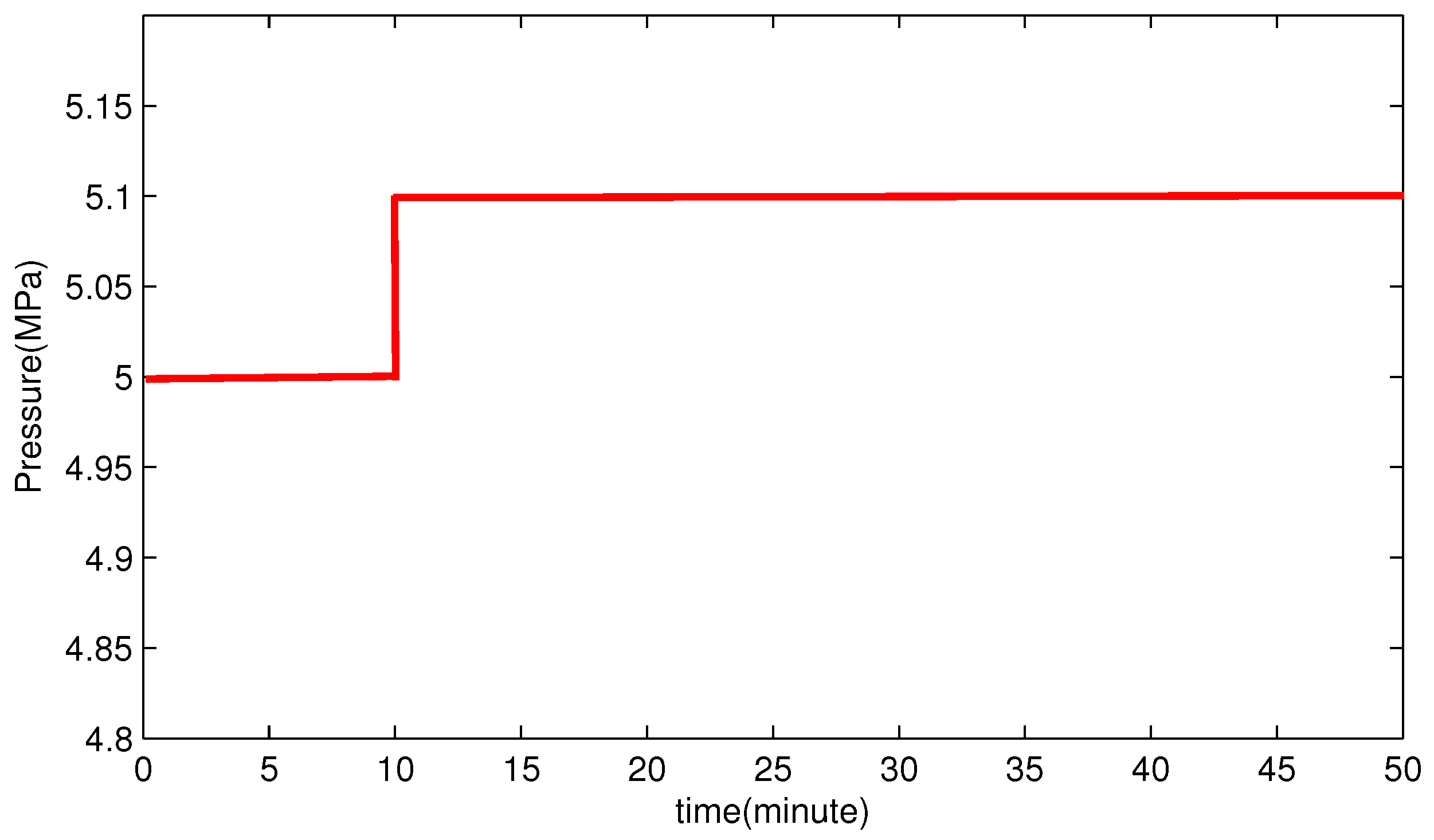
In order to visualize the basic performance of the models, the classical step change of the input variable (inlet pressure) was used as the external signal of the systems, as shown in Figure 3.

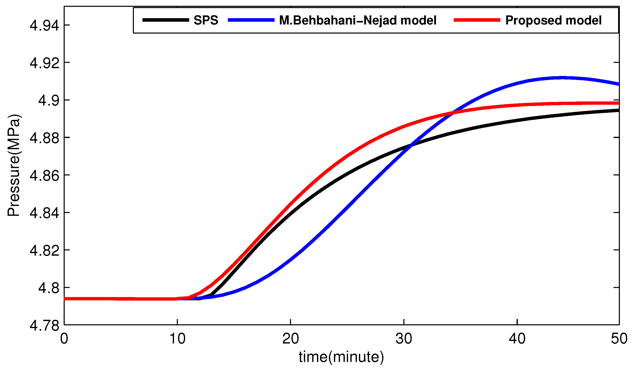
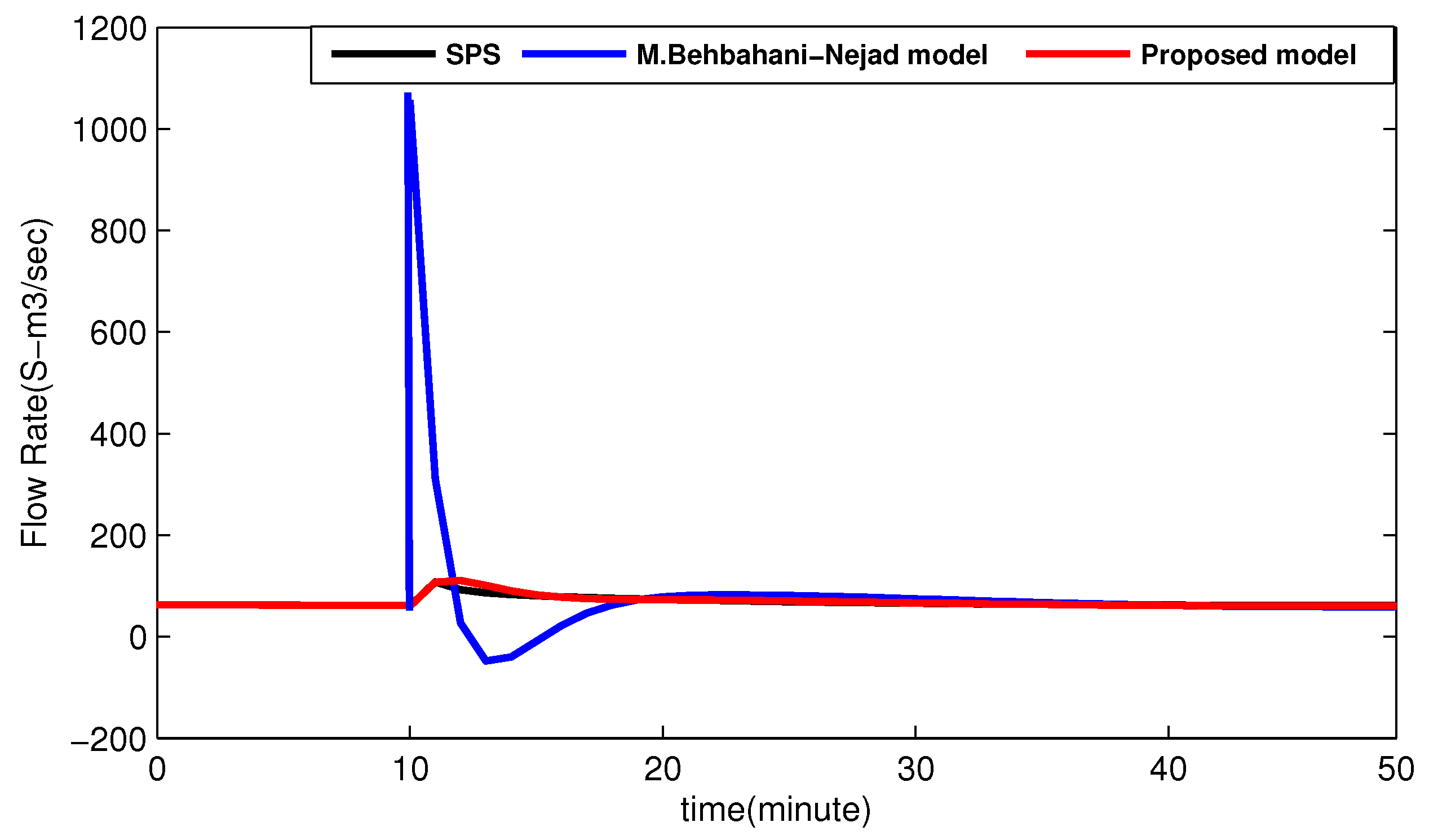
The parameters of the pipeline are shown in

Table 1. The basic parameters of the pipeline used in Example I.

Length (km)	Diameter (mm)	Temperature (${}^{\circ }$C)	Specific Gravity (-)	Roughness (mm)
60	660	21	0.55	0.012

. The initial inlet pressure was 5 MPa, and the initial flow rate was 60 N· m${}^3$/s. Here, it should be noticed that the flow rate in the state space model is the mass flow rate. In addition, there is a conversion coefficient between the volume flow rate and the mass flow rate. Figure 4 and Figure 5 show the responses of the outlet pressure and inlet flow rate of different models when the inlet pressure step changed from $5.0$ MPa to $5.1$ MPa. It should be noticed that

• The final pressure was $4.87$ MPa;
• There was a delay of about 200 s in the models;
• Our model was closer to the SPS simulation result;
• There was no sharp impulse of flow rate change in our model as in the SPS result.

Remark 3.

The state space model describes the pipelines as lumped parameter systems with ODE models rather than distributed parameter systems with PDE models, while, in PDE models, the inlet flow rate changes slowly because it is determined by its upstream and downstream states. With direct transfer matrix $\mathbb{D}$ in Equation (31), as shown in reference [14], the inlet flow rate has a quick response to the inlet pressure because of the existence of the direct transfer matrix. The impulse is clearly seen in Figure 5. Matrix $\mathbb{D}$ was eliminated in our model which assures that the output variable and the behavior of the pipeline are decided by their entire states, as in lumped parameter models. The input variable is an excitation signal to change the states of the entire pipeline. The pipeline is an inertia system in nature, and that is the key reason why our model is closer to the SPS simulation results.

3.2. Example II—Response to Complicated Inputs

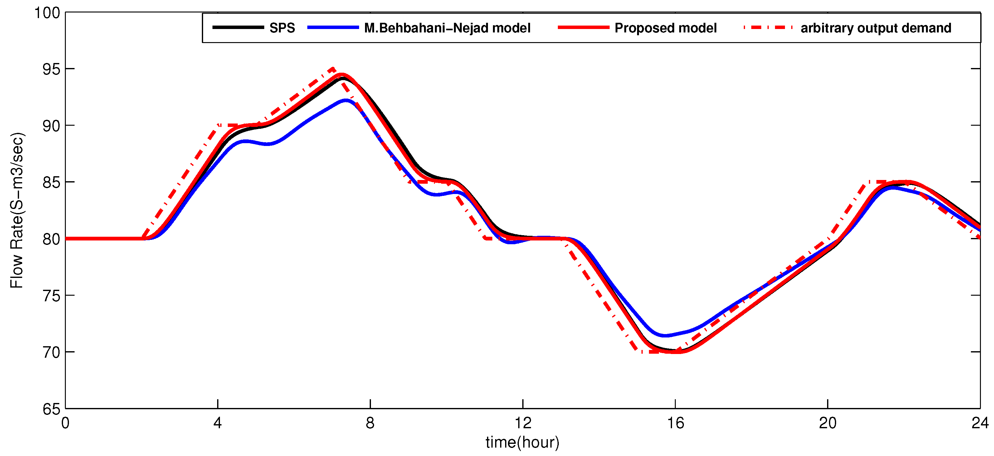
The quantity of daily use of natural gas is unpredictable and the outlet flow rate changes with time. In this part, a free change in outlet flow rate was used as the input to the system, which means the transportation of the pipeline must satisfy the needs of the market. This example was used to test the accuracy of our model in this scenario.

The parameters used for the pipeline were different from Example I, as listed in

Table 2. Basic Parameters of the Pipeline in Example II.

Length (km)	Diameter (mm)	Temperature (${}^{\circ }$C)	Specific Gravity (-)	Roughness (mm)
50	750	10	0.675	0.217

. The inlet pressure was kept at $3.0$ MPa during the simulation process. The flow rate was varied according to the consumption curve from the market as the dash-dot line in Figure 6. From the solid line in Figure 6, it can be seen that our model gave a perfect response to the input flow rate as SPS.

In practice, the outlet flow rate is decided by the market, as in Example II. The inlet pressure is under the control of the operators. The field operators are usually steps that change the set-points of the inlet pressure. Figure 6 shows the results of different models when the inlet pressure was set at $5.6$ MPa and the outlet flow rate followed the demand of the market as before.

3.3. Example III—A Pipeline Network

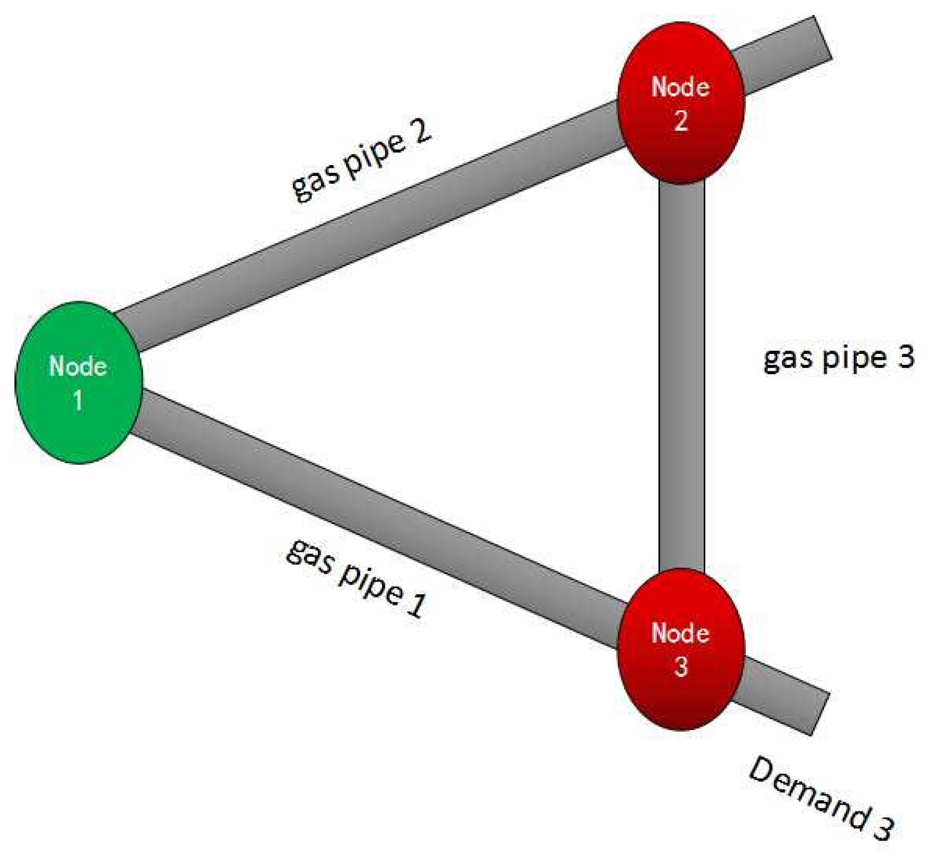
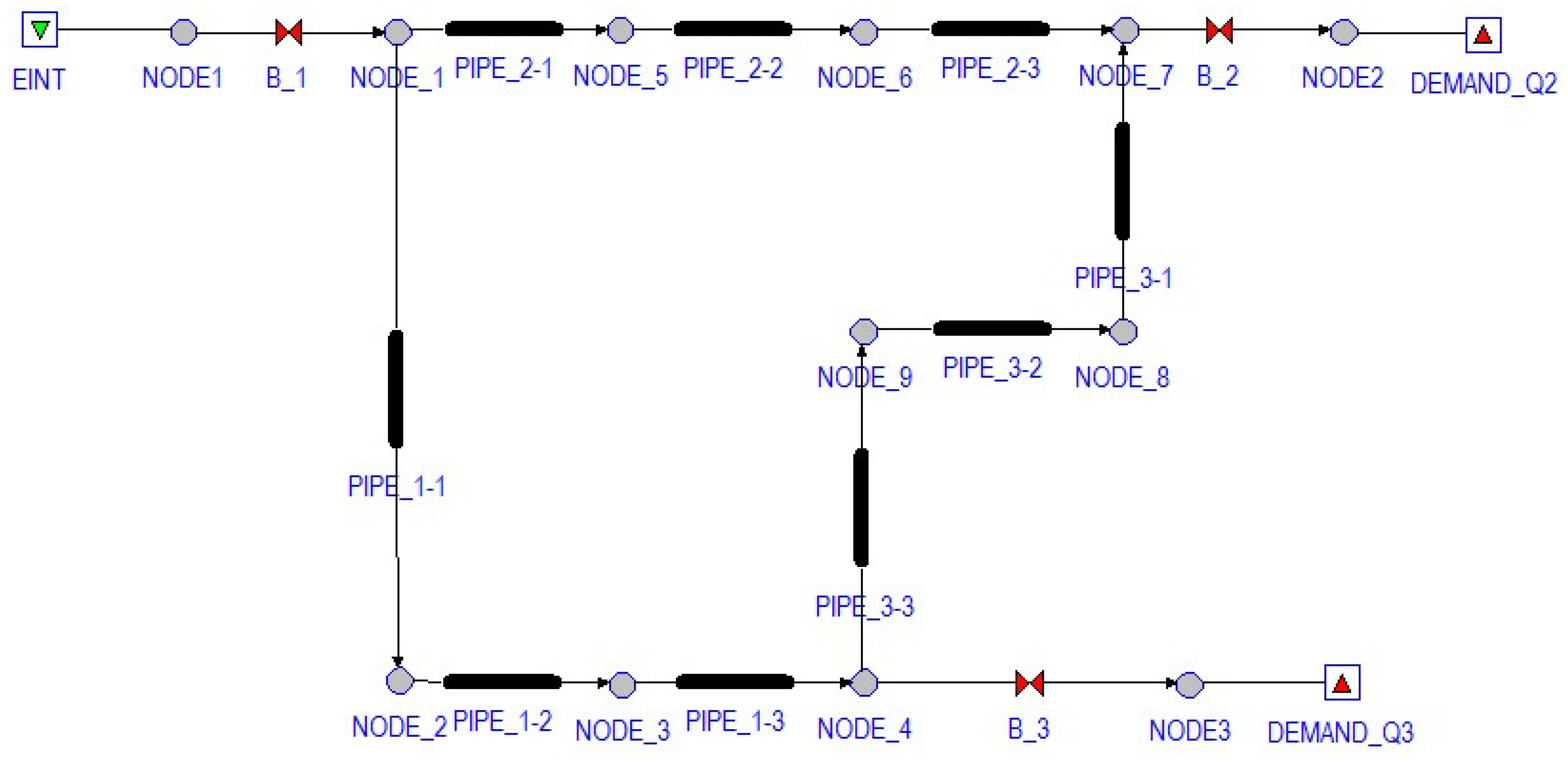
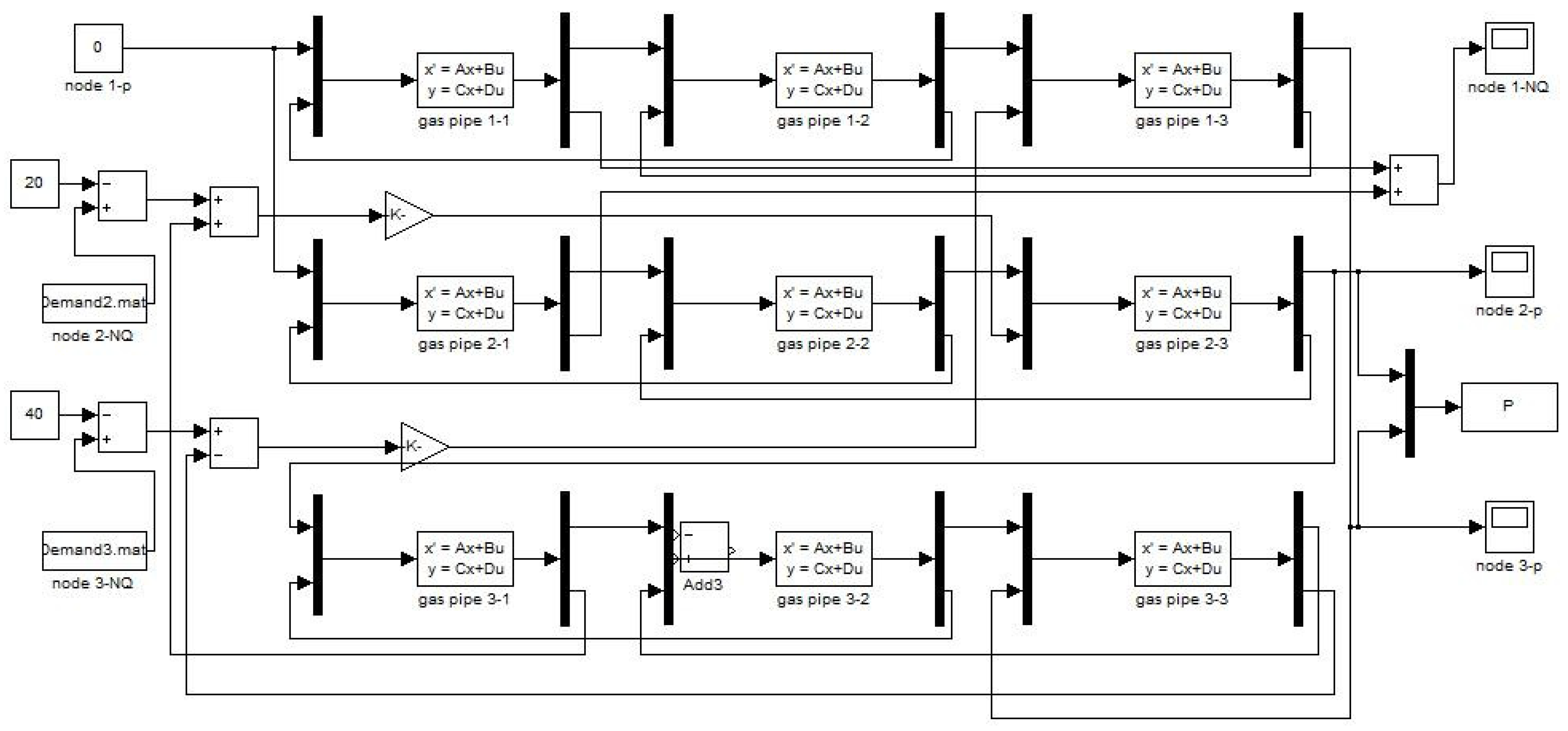
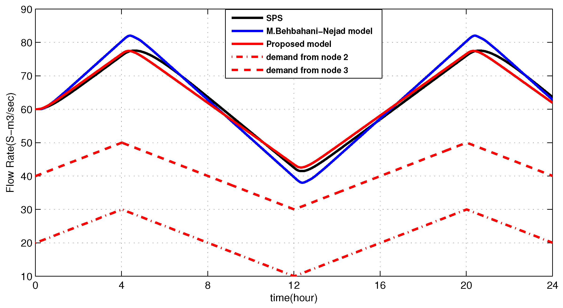
In this part, a simplified pipeline network was used, as shown in Figure 7, which consisted of three pipelines and two demand nodes (node 2 and node 3) supplied with gas by a single supply node (node 1). This network has been used as a benchmark in several pieces of literature [14]. Figure 8 is the corresponding SPS model of the network in Figure 7. Figure 9 show the block implementation of the state sapce model in MATLAB-Simulink. The geometrical data of the network is listed in

Table 3. The pipe’s geometrical data for a typical network.

From	To	Diameter (m)	Length (km)	Roughness (mm)
node	node
1	3	600	80	0.012
1	2	600	90	0.012
2	3	600	100	0.012

. The gas demands of node 2 and node 3 are represented by the dashed lines in Figure 10. The supply node (node 1) was pressure-controlled with the pressure maintained at $5.0$ MPa. The pipeline transported natural gas with a specific gravity of $0.6$ at $278\mathrm{K}$. The pipeline’s roughness value was assigned to be $0.012$ mm which is typical for transport pipelines.

The input ports specify the gas flow demand at node 2 and node 3 as well as the gas pressure at the inlet of the typical network. The outputs of the system are the gas pressure at node 2 and node 3, and the gas flow rate at the input of the network. The state space models of the pipeline network were built by connecting the state space model of Equation (31) and the state space model of Equation (33) in MATLAB-Simulink, as in Figure 9. The MATLAB required initial conditions for the transient simulation were obtained through a steady-state computation using the commercial software SPS. The state space models for each type of boundary condition were precalculated and input into the parameter boxes in Simulink blocks. In order to guarantee the accuracy of the simulation, pipe 1 was divided into 3 smaller segments, as were pipes 2 and 3. The numerical matrix of the state space model of the first segment of pipe 1 is listed in detail by Equation (43):

$$\begin{array}{c}\mathbb{A}=\left[\begin{array}{cccc}-0.0186& 1& 0& 0\\ -1.6556\times 10^{-4}& 0& 0& 0\\ 0& 0& -0.0186& 1\\ 0& 0& -1.6556\times 10^{-4}& 0\end{array}\right],\hfill \\ \mathbb{B}=\left[\begin{array}{cc}0& -130.6102\\ 1.6674\times 10^{-4}& -0.5036\\ 1.2300\times 10^{-5}& 0\\ 0& 1.6558\times 10^{-4}\end{array}\right],\hfill \\ \mathbb{C}=\left[\begin{array}{cccc}1& 0& 0& 0\\ 0& 0& 1& 0\end{array}\right].\hfill \end{array}$$

(43)

Figure 10 shows the inlet flow rate results of our model along with the obtained results of M.Behbahani-Nejad’s model [14] and the commercial software SPS. From Figure 10, one can observe that our model gives a better output of the input flow rate than SPS.

4. Conclusions

This paper gave a new lumped parameter model of a gas pipeline network. The model is able to describe the input–output dynamics of long natural gas pipelines without dividing them into small segments as usual. The three examples show the accuracy and the convenience of the model. The pipeline is an inertia dynamic system in nature. Our models eliminate direct matrix $\mathbb{D}$ in state space. This simplification avoids the quick responses of output variables which is more similar to the behavior of natural gas pipelines in practice. The models given in this paper are suitable for different combinations of input/output variables. The combinations of these state space models could describe different pipeline network structures. The state space model was derived from the transfer functions of dynamic gas flow. An explicit approximation for the Coolebrook–White equation was used during the derivation. Our model is more computationally efficient than traditional methods. It will be used in our future works for controllability analysis and controller design.

References

- Behrooz, H.; Boozarjomehry, R. Modeling and state estimation for gas transmission networks. J. Nat. Gas Sci. Eng. 2015, 22, 551–570. [Google Scholar] [CrossRef]
- Sukharev, M.; Kosova, K. A Parameter Identification Method for Natural Gas Supply Systems under Unsteady Gas Flow. Autom. Remote Control 2017, 78, 882–890. [Google Scholar] [CrossRef]
- Modisette, J. State Estimation of Pipeline Models using the Ensemble Kalman Filter. In Proceedings of the PSIG Annual Meeting, Prague, Czech Republic, 16–19 April 2013. [Google Scholar]
- Modisette, J. State Estimation in Online Models. In Proceedings of the PSIG Annual Meeting, Galveston, TX, USA, 12–15 May 2009. [Google Scholar]
- Szoplik, J. Improving the natural gas transporting based on the steady state simulation results. Energy 2016, 109, 105–116. [Google Scholar] [CrossRef]
- Aalto, H. Transfer Functions for Natural Gas Pipeline Systems. IFAC Proc. Vol. 2008, 41, 889–894. [Google Scholar] [CrossRef]
- Ibraheem, S.; Adewumi, M. Higher-resolution numerical solution for 2-D transient natural gas pipeline flows. In Proceedings of the SPE Gas Technology Symposium, Calgary, AB, Canada, 28 April–1 May 1996; pp. 473–482. [Google Scholar]
- Sanada, K.; Kitagawa, A. Robust control of a closed-loop pressure control system considering pipeline dynamics. Trans. Jpn. Soc. Mech. Eng. C 2011, 3, 3559–3566. [Google Scholar] [CrossRef]
- Uilhoorn, F. State-space estimation with a Bayesian filter in a coupled PDE system for transient gas flows. Appl. Math. Model. 2015, 39, 682–692. [Google Scholar] [CrossRef]
- Alamian, R.; Behbahani-Nejad, M.; Ghanbarzadeh, A. A state space model for transient flow simulation in natural gas pipelines. J. Nat. Gas Sci. Eng. 2012, 9, 51–59. [Google Scholar] [CrossRef]
- Herran-Gonzalez, A.; Cruz, J.; Andres-Toro, B.; Risco-Martín, J.L. Modeling and simulation of a gas distribution pipeline network. Appl. Math. Model. 2009, 33, 1584–1600. [Google Scholar] [CrossRef]
- Behbahani-Nejad, M.; Bagheri, A. The accuracy and efficiency of a MATLAB-Simulink library for transient flow simulation of gas pipelines and networks. J. Pet. Sci. Eng. 2010, 70, 256–265. [Google Scholar] [CrossRef]
- Reddy, H.; Narasimhan, S.; Bhallamudi, S. Simulation and State Estimation of Transient Flow in Gas Pipeline Networks Using a Transfer Function Model. Ind. Eng. Chem. Res. 2006, 45, 3853–3863. [Google Scholar] [CrossRef]
- Behbahani-Nejad, M.; Shekari, Y. Reduced order modeling of natural gas transient flow in pipelines. Int. J. Eng. Appl. Sci. 2008, 5, 148–152. [Google Scholar]
- White, F. Fluid Mechanics; McGraw-Hill: New York, NY, USA, 1986. [Google Scholar]
- Kralik, J.; Stiegler, P.; Vostry, Z.; Zavorka, J. Dynamic Modeling of Large-Scale Networks with Application to Gas Distribution, 1st ed.; Institution of Information Theory and Automation of the Czechoslovak Academy of Sciences: Prague, Czechoslovakia, 1998. [Google Scholar]
- Aalto, H. Model reduction for natural gas pipeline systems. Large Scale Complex Syst. Theory Appl. 2010, 43, 468–473. [Google Scholar] [CrossRef]
Figure 1.
Bode plot of and in Equation (23).
Figure 2.
Bode plot of and in Equation (24).
Figure 3.
A gas pipe with step variation for inlet pressure.
Figure 4.
Outlet pressure changes with time.
Figure 5.
Inlet flow rate changes with time.
Figure 6.
Figure 7.
Topology of the typical network.
Figure 8.
SPS (Stoner Pipeline Simulator) model of the typical network.
Figure 9.
MATLAB-Simulink model of the typical network.
Figure 10.
Demands for node 2 and node 3 and inlet flow rate for node 1.