Energy Loss Allocation in Smart Distribution Systems with Electric Vehicle Integration

Abstract

This paper presents a three-phase loss allocation procedure for distribution networks. The key contribution of the paper is the computation of specific marginal loss coefficients (MLCs) per bus and per phase expressly considering non-linear load models for Electric Vehicles (EV). The method was applied in a unbalanced 12.47 kV feeder with 12,780 households and 1000 EVs under peak and off-peak load conditions. Results obtained were also compared with the traditional roll-in embedded allocation procedure (pro rata) using non-linear and standard constant power models. Results show the influence of the non-linear load model in the energy losses allocated. This result highlights the importance of considering an appropriate EV load model to appraise the overall losses encouraging the use and further development of the methodology

1. Introduction

Electrical distribution systems are immersed in a deep process of transformation becoming very different from what they used to be. The increasing penetration of distributed generators, the expected connection of a large amount of plug-in electric vehicles (EV) and the adoption of advanced metering and communication infrastructure (AMI) are creating new challenges for regulators. The widespread integration of EVs into existing distribution networks will increase feeder demands and therefore will produce rising energy losses [1]. Moreover, due to the different nature of EV loads (slow and fast battery charging stations), one-phase and two-phase connections may increase system unbalance producing additional losses. A recent study about the impact of the placement of fast charging stations in distribution systems showed a power loss increase of 85% [2] with respect to a base layer with no EV integration. Therefore, some conceptual and regulatory questions can be raised about the EV impacts on the increase of energy losses in distribution networks:

• How much should an EV load pay for the incremental losses in the grid [3]?
• Should incremental losses produced by EVs connected to fast and slow charging stations be allocated in a proportional manner among all distribution loads [3]?
• Can a price signal for losses (sent in real-time via AMI and smart metering) force the EV loads to provide volt/var support in order to improve voltage profile and reduce system losses [4]?

These regulatory aspects can be addressed by means of a cost-reflective energy loss allocation procedure in order to send economical signals to consumers and producers with the aim of improving overall performance of the system. The energy loss allocation is not new issue in electricity markets. It has been widely treated in the literature mainly at transmission systems [5] and more recently in distribution systems considering increasing integration of distributed generators [6]. In general, the majority of the loss allocation procedures discussed in the literature are based upon positive-sequence power flow models with balanced power injections where all loads are modeled using standard constant real and reactive power (PQ) models [7,8,9]. In this case, load demands are not affected by voltage fluctuations (constant power load models).

Power loss allocation constitutes an important strategy to determine locational prices at distribution level in order to send efficiency economical signals to demands [10,11] and distributed generators [12] at distribution level. Recent contributions are devoted to extending positive-sequence power loss allocation procedures into unbalanced three phase domain [13,14]. Based upon the calculation of sensitivity loss factors in the context of the optimal power flow problem, some work is carried out to assess locational marginal pricing and EV charging management [15].

However, previous loss allocation methods discussed in literature only consider constant power loads and do not take into account non-linear nature of EV loads [16]. System unbalance produced by fast charging stations with single- and two-phase connections as well as the above-mentioned voltage dependence justify the development of detailed three-phase loss allocation procedure to assess the impact of EV loads on incremental losses.

To fill the research gap, this paper presents three-phase loss allocation procedure for distribution networks that expressly incorporates a non-linear load model. This model can be adjusted as exponential, constant power, current and impedance depending on EV load parametrization. The proposed procedure is based on the computation of specific marginal loss coefficients (MLCs) per bus and phase.

The method is illustrated in a unbalanced 12.47 kV feeder with 12,780 residential customers. Daily energy losses were allocated considering five levels of EV penetration: 200, 400, 800 and 1000 units corresponding to 5%, 10%, 15%, 20% and 25% of consumption without EV presence. Two operational scenarios with two different type of charging stations are studied. A 3.75 kW slow battery charger from 0:00 to 8:00 and a 7.5 kW fast charger from 18:00 to 22:00. Results obtained were also compared with traditional roll-in embedded allocation method (pro rata) [17]. Finally, a sensitivity analysis was performed to compare the results with ones obtained using a standard constant power model.

This paper is organized as follows. Section 2 is devoted to present the proposed method. Section 3 defines the case study. Section 4 discusses the results. Section 5 draws the conclusions.

2. The Energy Loss Allocation Model

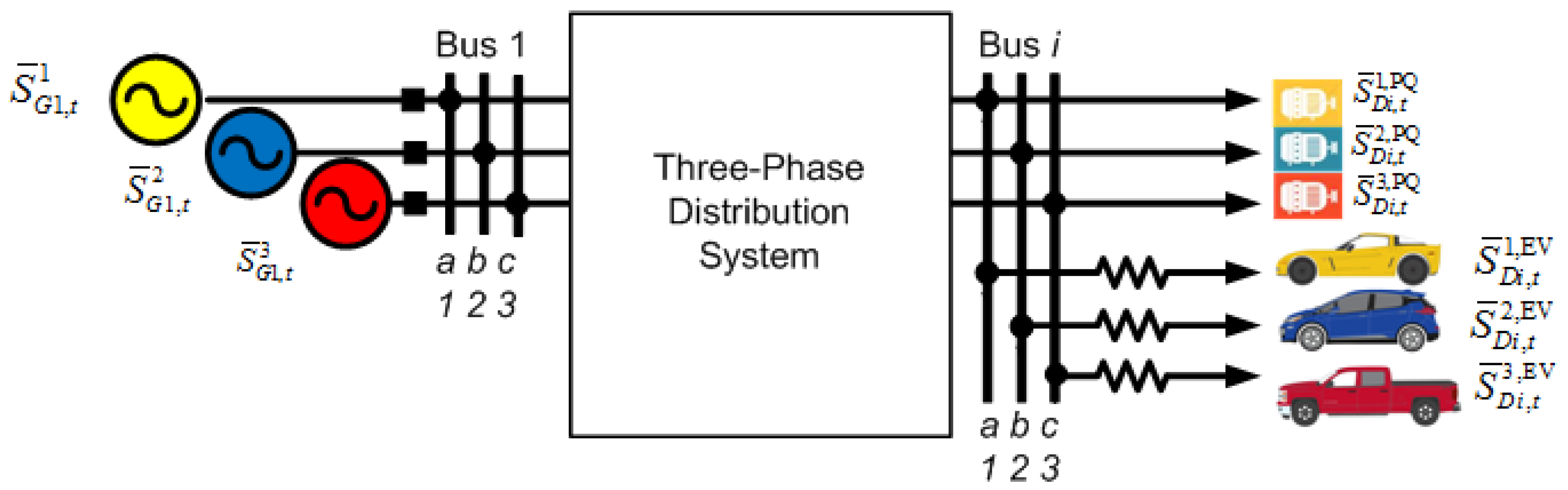
The system model is based upon a typical n buses three-phase unbalanced distribution network with two types of loads connected at each bus i: residential loads and non linear EV loads, as shown in Figure 1.

In this paper, we assess the energy loss allocation problem among all loads considering a passive network with EV integration. The model can be extended to active networks with distributed generation and bidirectional EV injections. However, our purpose here is to analyze technical and economical impacts of EV’s connected to slow and fast charging stations under peak and off-peak conditions.

2.1. PQ and EV Load Modeling

Distribution loads characteristics depend on the share of different demand types (industrial, commercial and residential) and can be modeled in a more complex way as a mix of different voltage–current models as constant impedance, constant current and constant power. For the sake of simplicity, in this paper, all residential demands are regarded as constant loads. This means that constant loads such as induction motors are predominant at demand side. In the reminder of the paper, these constant power loads are denoted as constant real and reactive power (PQ) loads. Constant power loads do not depend on voltage fluctuations.

Then, at given time t of a period T, the apparent power of a PQ load at bus i and phase p is denoted as:

$${\overline{S}}_{Di,t}^{p,PQ}=P_{Di,t}^{p,PQ}+j{Q}_{Di,t}^{p,PQ}i=2,\dots ,np=1,2,3t=1,\dots ,T$$

(1)

where $P_{Di,t}^{p,PQ}$ and $Q_{Di,t}^{p,PQ}$ are the real and the reactive power of a PQ load. No loads are connected at source bus i = 1.

The second type of load considered in the formulation is the aggregation of a number of EVs connected to a given bus i. There are several load models for EVs. Many parametric models are based on real power injections [18,19] considering a power factor equal to 1. Without loss of generality, due to regulatory and operational reasons [20], EVs can be requested to provide voltage and reactive power support. In this case, apparent, real and reactive power are modeled using a non-linear function [21] and a fixed power factor angle ${\varphi }_{Di,t}^p$, respectively:

$${\overline{S}}_{Di,t}^{p,EV}=P_{Di,t}^{p,EV}+j{Q}_{Di,t}^{p,EV}i=2,\dots ,np=1,2,3t=1,\dots ,T$$

(2)

where the real power demanded by aggregate EVs at time t, bus i and phase p is given by

$$P_{Di,t}^{p,EV}=P_o[a+b(\frac{V_i^p}{V_o})]{}^{\alpha }i=2,\dots ,np=1,2,3t=1,\dots ,T$$

(3)

where $a+b$ = 1.

The reactive power demanded by EVs at time t, bus i and phase p is given by

$$Q_{Di,t}^{p,EV}=P_{Di,t}^{p,EV}tan{\varphi }_{Di,t}^p=\sqrt{{(S_{Di,t}^{p,EV})}^2-{(P_{Di,t}^{p,EV})}^2}i=2,\dots ,np=1,2,3t=1,\dots ,T$$

(4)

Parameters a, b and $\alpha$ depend on EV charger characteristics and the equivalent resistance R between each connection outlet at low voltage and the system bus i. $P_o$ and $V_o$ are the nominal power and nominal voltage. Some values of the EV parameters can be found in [21]. Note that, if $\alpha$ = 0, the model reflects a PQ load; if $\alpha$ = 1, the model reflects a constant current load; and, if $\alpha$ = 2, the model reflects a constant impedance load. In general, EV load parametrization leads to negative values of $\alpha$ as indicated by [21].

At given time t, the system power balance is given by:

$$\sum _{p=1}^3{\overline{S}}_{G1,t}^p=\Delta {\overline{S}}_t+\sum _{i=2}^n\sum _{p=1}^3{\overline{S}}_{Di,t}^{p,PQ}+\sum _{i=2}^n\sum _{p=1}^3{\overline{S}}_{Di,t}^{p,EV}t=1,\dots ,T$$

(5)

where ${\overline{S}}_{Gi,t}^p$ is the power injected at reference bus 1 at Phases 1, 2 and 3, and $\Delta {\overline{S}}_t$ is the total apparent losses. Total apparent losses can be split into real losses $\Delta P_t=Re(\Delta {\overline{S}}_t)$ and reactive losses $\Delta Q_t=Im(\Delta {\overline{S}}_t)$.

Total real energy consumed by PQ and EV loads at each bus i during a period T, i.e., 24 h are given by:

$$W_{Di}^{PQ}=\sum _{t=1}^T\sum _{p=1}^3{P}_{Di,t}^{p,PQ};W_{Di}^{EV}=\sum _{t=1}^T\sum _{p=1}^3{P}_{Di,t}^{p,EV}i=2,\dots ,n$$

(6)

Total real energy delivered by the source bus 1 is given by:

$$W_1=\sum _{t=1}^T\sum _{p=1}^3{P}_{G1,t}^p$$

(7)

The system real energy balance is given by:

$$W_1=\sum _{i=2}^n{W}_{Di}^{PQ}+\sum _{i=2}^n{W}_{Di}^{EV}+\Delta W$$

(8)

and, then total real energy losses are

$$\Delta W=\sum _{t=1}^T\sum _{p=1}^3{P}_{G1,t}^p-\sum _{t=1}^T\sum _{i=2}^n\sum _{p=1}^3{P}_{Di,t}^{p,PQ}-\sum _{t=1}^T\sum _{i=2}^n\sum _{p=1}^3{P}_{Di,t}^{p,EV}$$

(9)

where $\Delta W$ is the system real energy losses to be allocated between all network users (PQ and EV loads) during a defined time interval T.

2.2. Evaluation of Power Losses to Be Allocated among the Network Users

The power and losses to be allocated can be evaluated from the solution of the standard three-phase power flow problem. The solution comprises all system voltages (magnitude and angle) except the voltages fixed at reference. There are several methods to solve this issue. In general, when all loads are regarded as PQ constant, Newton–Raphson method can be applied either by its complete formulation [22] or decoupled formulation [23]. Other Gauss-based methods suitable to be applied at distribution level can be used instead [24,25].

For non-linear loads (such as EVs), if the three-phase admittance matrix ($Y_{BUS}$) is known, the power flow solution can be obtained at given operating point (time t) from a set of $3(n-1)$ equations and $3(n-1)$ unknowns:

$$P_{i,t}^p=-P_{Di,t}^{p,PQ}-P_{Di,t}^{p,EV}\left(V_{i,t}^p\right)=V_{i,t}^p\sum _{k=1}^n\sum _{p=1}^3\sum _{m=1}^3{V}_{k,t}^m[G_{ik}^{pm}cos{\theta }_{ik,t}^{pm}+B_{ik}^{pm}sin{\theta }_{ik,t}^{pm}]\forall i\ne 1,p$$

(10)

where ${\theta }_{ik,t}^{pm}={\theta }_{i,t}^p-{\theta }_{k,t}^m$.

$$Q_{i,t}^p=-Q_{Di,t}^{p,PQ}-Q_{Di,t}^{p,EV}\left(V_{i,t}^p\right)=V_{i,t}^p\sum _{k=1}^n\sum _{p=1}^3\sum _{m=1}^3{V}_{k,t}^m[G_{ik}^{pm}sin{\theta }_{ik,t}^{pm}-B_{ik}^{pm}cos{\theta }_{ik,t}^{pm}]\forall i\ne 1,p$$

(11)

where $P_{Di,t}^{p,PQ}$ and $Q_{Di,t}^{p,PQ}$ are constant parameters, and $P_{Di,t}^{p,EV}$ and $Q_{Di,t}^{p,EV}$ are non-linear functions depending on its own voltage magnitude as given in Equations (3) and (4). At reference bus 1, voltage magnitude and angle are known for all phases: ${\overline{V}}_1^1=V_1{e}^{j0}$, ${\overline{V}}_1^2=V_1{e}^{j\frac{-2\pi }{3}}$ and ${\overline{V}}_1^3=V_1{e}^{j\frac{2\pi }{3}}$ where $V_1$ is the voltage magnitude at reference bus 1. Then, once the power flow algorithm is applied to solve the set of Equations (10) and (11), the solution ${\mathbf{x}}_{\mathbf{t}}$ = $[V_{1,t}^1,\dots ,V_{i,t}^p,\dots ,V_{n,t}^3;{\theta }_{1,t}^1,\dots ,{\theta }_{i,t}^p,\dots ,{\theta }_{n,t}^3]$ is evaluated in the following expression in order to get the real system power losses:

$$\Delta P_t=\sum _{i=1}^n\sum _{k=1}^n\sum _{p=1}^3\sum _{m=1}^3{V}_{i,t}^p{V}_{k,t}^m[G_{ik}^{pm}cos{\theta }_{ik,t}^{pm}+B_{ik}^{pm}sin{\theta }_{ik,t}^{pm}]t=1,\dots ,T$$

(12)

The $G_{ik}^{pm}$ and $B_{ik}^{pm}$ entries correspond to the conductance and susceptance terms of the admittance matrix ($Y_{BUS}$) between phase p at bus i and phase m at bus k.

The total real energy to allocate among network users is given by:

$$\Delta W=\sum _{t=1}^T\Delta P_t$$

(13)

2.3. Energy Loss Allocation Procedures

We consider two procedures to allocate energy losses among network PQ loads and non-linear EV loads:

• The proposed marginal allocation procedure per bus and per phase
• The standard pro rata or proportional allocation for comparison purposes [17]

2.3.1. Marginal Loss Allocation

Distribution losses can be allocated among network users is means of the sensitivity factors also known as marginal loss coefficients (MLCs) [26]. This allocation process yields on different charges depending on the effect of each user on overall losses. Thus, the power losses allocated or assigned to PQ loads located at bus i, phase p, at time t are:

$$L_{Di,t}^{M,p,PQ}=k_{r,t}\left|\right|ML{C}_{Di,t}^p\left|\right|P_{Di,t}^{p,PQ}i=2,\dots ,np=1,2,3t=1,\dots ,T$$

(14)

and power losses allocated to EV loads located at bus i, phase p, at time t are:

$$L_{Di,t}^{M,p,EV}=k_{r,t}\left|\right|ML{C}_{Di,t}^p\left|\right|P_{Di,t}^{p,EV}(V_{i,t}^p)i=2,\dots ,np=1,2,3t=1,\dots ,T$$

(15)

It must be highlighted that the application of MLCs produce an over-recovery of losses [27]. This is due to the nonlinear nature (quadratic) of losses. To reconcile the total power losses, i.e., recover the exact amount of grid losses, it is necessary to multiply the allocated power losses by a reconciliation factor $k_{r,t}$. This factor avoids a over recovery of power losses at each time t:

$$k_{r,t}=\frac{\Delta P_t}{{\sum }_{i=2}^n{\sum }_{p=1}^3\left|\right|ML{C}_{Di,t}^p\left|\right|P_{Di,t}^{p,EV}(V_{i,t}^p)}t=1,\dots ,T$$

(16)

The total real energy losses allocated to loads at bus i and phase p are:

$$A_{Di}^{M,p,PQ}=\sum _{t=1}^T{L}_{Di,t}^{M,p,Q};A_{Di}^{M,p,EV}=\sum _{t=1}^T{L}_{Di,t}^{M,p,EV}i=2,\dots ,np=1,2,3$$

(17)

The total real energy losses allocated to PQ and EV loads under proposed marginal approach are:

$$A_D^{M,PQ}=\sum _{t=1}^T\sum _{i=2}^n\sum _{p=1}^3{A}_{Di,t}^{M,p,PQ};A_D^{M,EV}=\sum _{t=1}^T\sum _{i=2}^n\sum _{p=1}^3{A}_{Di,t}^{M,p,EV}$$

(18)

Considering that losses are recovered using a 24-h day-ahead spot price ${\rho }_t$ in USD/MWh, the payments per losses of loads at bus i and phase p are:

$${\mathsf{\Omega }}_{Di}^{M,p,PQ}=\sum _{t=1}^T{\rho }_t{L}_{Di,t}^{M,p,PQ};{\mathsf{\Omega }}_{Di}^{M,p,EV}=\sum _{t=1}^T{\rho }_t{L}_{Di,t}^{M,p,EV}i=2,\dots ,np=1,2,3$$

(19)

Global energy loss payments under the marginal approach are:

$${\mathsf{\Omega }}_D^{M,PQ}=\sum _{t=1}^T\sum _{i=2}^n\sum _{p=1}^3{\rho }_t{L}_{Di,t}^{M,p,PQ};{\mathsf{\Omega }}_D^{M,EV}=\sum _{t=1}^T\sum _{i=2}^n\sum _{p=1}^3{\rho }_t{L}_{Di,t}^{M,p,EV}$$

(20)

Determining the three-phase MLCs: To get the marginal loss coefficients, we can solve the network stating an optimization problem as follows:

$$\begin{array}{c}min\Delta P_t=\sum _{i=1}^n\sum _{k=1}^n\sum _{p=1}^3\sum _{m=1}^3{V}_{i,t}^p{V}_{k,t}^m[G_{ik}^{pm}cos{\theta }_{ik,t}^{pm}+B_{ik}^{pm}sin{\theta }_{ik,t}^{pm}]t=1,\dots ,T\hfill \end{array}$$

(21)

subject to:

$$\begin{array}{c}{P}_{i,t}^p=-P_{Di,t}^{p,PQ}-P_{Di,t}^{p,EV}(V_{i,t}^p)=V_{i,t}^p\sum _{k=1}^n\sum _{p=1}^3\sum _{m=1}^3{V}_{k,t}^m[G_{ik}^{pm}cos{\theta }_{ik,t}^{pm}+B_{ik}^{pm}sin{\theta }_{ik,t}^{pm}]\forall i\ne 1\hfill \end{array}$$

(22)

$$\begin{array}{c}{Q}_{i,t}^p=-Q_{Di,t}^{p,PQ}-Q_{Di,t}^{p,EV}(V_{i,t}^p)=V_{i,t}^p\sum _{k=1}^n\sum _{p=1}^3\sum _{m=1}^3{V}_{k,t}^m[G_{ik}^{pm}sin{\theta }_{ik,t}^{pm}-B_{ik}^{pm}cos{\theta }_{ik,t}^{pm}]\forall i\ne 1\hfill \end{array}$$

(23)

As the formulation has the same number of equations and unknowns, the optimization problem is determined. The results coincide with the power flow solution. However, it should be highlighted that the Lagrange multiplier associated with Equation (22) for bus i and phase p is just the marginal loss coefficient $ML{C}_{Di,t}^p$:

$$ML{C}_{Di,t}^p=\frac{\partial \Delta P_t}{\partial P_{i,t}^p}i=2,\dots ,np=1,2,3t=1,\dots ,T$$

(24)

Lagrange multipliers are usually provided by any optimization package. In the test case we used the fmincon optimization solver of Matlab (version R2017, v.9.2) to get the MLCs and to illustrate the application of the method.

2.3.2. Pro Rata or Proportional Allocation

Pro rata method describes a proportionate allocation of losses among all loads according the amount of power demand at each bus and phase. It consists of assigning an amount to a fraction according to its share of the whole [17]. Thus, the power losses allocated to PQ loads at bus i, phase p and time t are:

$$L_{Di,t}^{P,p,PQ}=\Delta P_t\frac{P_{Di,t}^{p,PQ}}{{\sum }_{i=2}^n{\sum }_{p=1}^3{P}_{Di,t}^{p,PQ}+{\sum }_{i=2}^n{\sum }_{p=1}^3{P}_{Di,t}^{p,EV}\left(V_{i,t}^p\right)}i=2,\dots ,np=1,2,3t=1,\dots ,T$$

(25)

and power losses to be allocated to EV loads located at bus i, phase p, at time t are:

$$L_{Di,t}^{P,p,EV}=\Delta P_t\frac{P_{Di,t}^{p,EV}\left(V_{i,t}^p\right)}{{\sum }_{i=2}^n{\sum }_{p=1}^3{P}_{Di,t}^{p,PQ}+{\sum }_{i=2}^n{\sum }_{p=1}^3{P}_{Di,t}^{p,EV}\left(V_{i,t}^p\right)}i=2,\dots ,np=1,2,3t=1,\dots ,T$$

(26)

The total real energy losses to be allocated to loads at bus i and phase p are:

$$A_{Di}^{P,p,PQ}=\sum _{t=1}^T{L}_{Di,t}^{P,p,Q};A_{Di}^{P,p,EV}=\sum _{t=1}^T{L}_{Di,t}^{P,p,EV}i=2,\dots ,np=1,2,3$$

(27)

The total real energy losses allocated to PQ and EV loads under pro rata approach are:

$$A_D^{P,PQ}=\sum _{t=1}^T\sum _{i=2}^n\sum _{p=1}^3{A}_{Di,t}^{P,p,PQ};A_D^{P,EV}=\sum _{t=1}^T\sum _{i=2}^n\sum _{p=1}^3{A}_{Di,t}^{P,p,EV}$$

(28)

Considering that losses are recovered using a uniform price $\rho$ in USD/MWh, the payments per losses of loads at bus i and phase p are:

$${\mathsf{\Omega }}_{Di}^{P,p,PQ}=\rho A_{Di}^{P,p,PQ};{\mathsf{\Omega }}_{Di}^{P,p,EV}=\rho A_{Di}^{P,p,EV}i=2,\dots ,np=1,2,3$$

(29)

Global energy loss payments under the pro rata approach are:

$${\mathsf{\Omega }}_D^{P,PQ}=\sum _{i=2}^n\sum _{p=1}^3\rho A_{Di}^{P,p,PQ};{\mathsf{\Omega }}_D^{PEV}=\sum _{i=2}^n\sum _{p=1}^3\rho A_{Di}^{P,p,EV}$$

(30)

3. Case Study

The proposed energy loss allocation procedure was applied in the well-known 21-bus Kersting NEV test system [28]. This system has a three-phase main feeder connected to an ideal 12.47 kV (line-to-line) source. The feeder has 1828.8 m (6000 ft) long and an average pole span of 91.44 m (300 ft). The original test case has a unique load concentrated at the ending node. We modified the loading scheme by introducing a uniformly increasing load in each phase from bus 2 to bus 21 according to

Table 1. Base load: No EV connected, only PQ loads.

Bus	Total		Phase 1		Phase 2		Phase 3
	${\mathit{W}}_{\mathit{Di}}^{\mathit{PQ}}$	${\mathit{P}}_{\mathit{Di}}^{\mathit{PQ}}$	${\mathit{W}}_{\mathit{Di}}^{\mathbf{1},\mathit{PQ}}$	${\mathit{P}}_{\mathit{Di}}^{\mathbf{1},\mathit{PQ}}$	${\mathit{W}}_{\mathit{Di}}^{\mathbf{2},\mathit{PQ}}$	${\mathit{P}}_{\mathit{Di}}^{\mathbf{2},\mathit{PQ}}$	${\mathit{W}}_{\mathit{Di}}^{\mathbf{3},\mathit{PQ}}$	${\mathit{P}}_{\mathit{Di}}^{\mathbf{3},\mathit{PQ}}$
	MW·h/day	kW	MW·h/day	kW	MW·h/day	kW	MWh/day	kW
2	0.6	0.04	0.2	0.01	0.2	0.02	0.2	0.01
3	1.2	0.08	0.4	0.03	0.5	0.03	0.4	0.02
4	1.8	0.12	0.6	0.04	0.7	0.05	0.5	0.04
5	2.4	0.16	0.8	0.05	0.9	0.06	0.7	0.05
6	3.0	0.20	1.0	0.07	1.1	0.08	0.9	0.06
7	3.7	0.24	1.2	0.08	1.4	0.09	1.1	0.07
8	4.3	0.28	1.4	0.09	1.6	0.11	1.2	0.08
9	4.9	0.32	1.6	0.11	1.8	0.12	1.4	0.10
10	5.5	0.37	1.8	0.12	2.1	0.14	1.6	0.11
11	6.1	0.41	2.0	0.14	2.3	0.15	1.8	0.12
12	6.7	0.45	2.2	0.15	2.5	0.17	2.0	0.13
13	7.3	0.49	2.4	0.16	2.7	0.18	2.1	0.14
14	7.9	0.53	2.6	0.18	3.0	0.20	2.3	0.15
15	8.5	0.57	2.8	0.19	3.2	0.21	2.5	0.17
16	9.1	0.61	3.0	0.20	3.4	0.23	2.7	0.18
17	9.7	0.65	3.2	0.22	3.6	0.24	2.9	0.19
18	10.3	0.69	3.4	0.23	3.9	0.26	3.0	0.20
19	11.0	0.73	3.6	0.24	4.1	0.27	3.2	0.21
20	11.6	0.77	3.8	0.26	4.3	0.29	3.4	0.23
21	12.2	0.81	4.0	0.27	4.6	0.30	3.6	0.24
Total	127.8	8.53	42.5	2.84	47.8	3.19	37.5	2.50

. The loading scheme considers a substation with four main feeders in a high density area. In this case, according to [29], the load increase is linear with respect to the distance. Then, source bus 1 has no load and the last bus 21 has the highest load value. For the sake of simplicity, only the main feeder is considered for the proposed analysis. Single phase derivations and laterals are neglected.

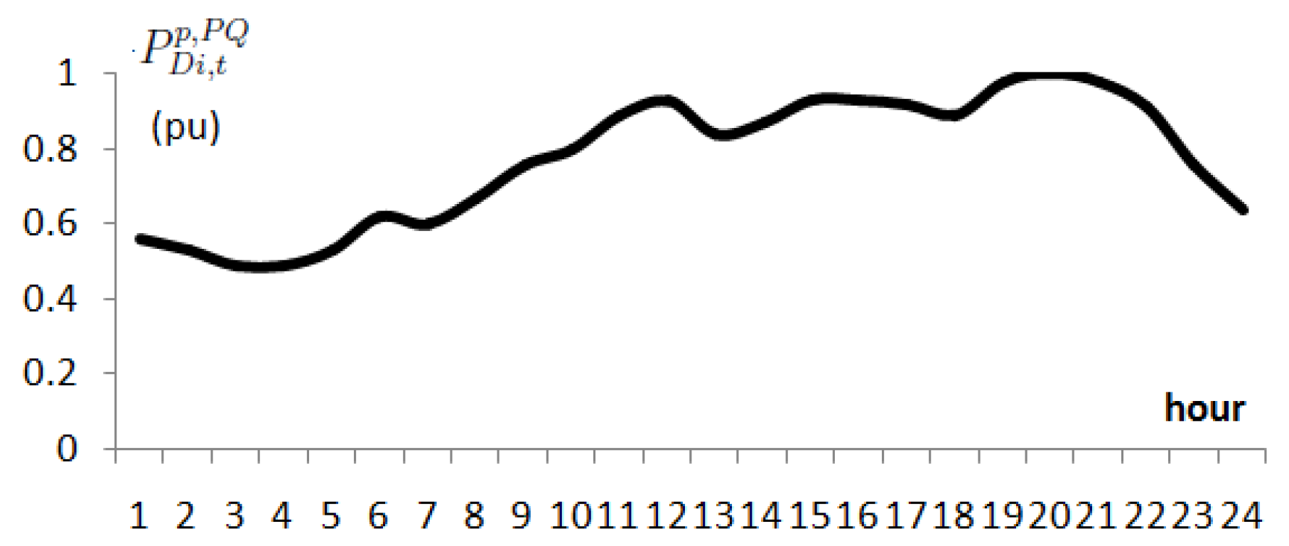
The last row of Table 1 corresponds to the sum of all energy consumptions at substation (bus 1) and the sum of all coincident demands flowing at main feeder (between buses 1 and 2). Total peak power flowing by the main feeder (bus 1) is 8526 kW at 20:00. Total three-phase load consumption is 127.8 MW·h/day, corresponding to 12,780 customers (each household consumes 10 kW·h/day, 300 kW·h/month with load factor 0.62). The 24-h real power load curve in p.u. for all buses and phases is depicted in Figure 2. For simplicity, all loads $P_{Di,t}^{p,PQ}$, $i=2,\dots ,21$, $p=1,2,3$, $t=1,\dots ,24$ have the same load curve. Then, all maximum demands are coincident at 20:00 but with different real power values per phase and bus (as shown in Table 1) ensuring unbalanced operation.

The network structure was scripted in OpenDSS (version 7.6.5.52, Electric Power Research Institute, Inc., Palo Alto, CA, USA) [30] (included in the Appendix A to extract the three-phase network model (admittance matrix). Power flow solution at base layer (with no EV penetration) showed that total peak power losses reach 115 kW at 20:00. Total energy losses are 1.33 MW·h/day (approximately 1.04% of total). The worst voltage drop is 3.69% at node 21 phase a.

In this paper, we do not emphasize on voltage profile results since our objective is to illustrate from conceptual viewpoint the proposed three-phase loss allocation procedure under specified operation battery charging schemes. There are other type studies, e.g., hosting capacity [31], where realistic operation schemes is addressed using Monte Carlo simulations with stochastic EV demands [32,33,34,35,36]. Thus, this work does not intend to replicate the probabilistic behavior of EV connection in a given period. Further research can be conducted to assess realistic loss allocation payments in a city and a country with specific patterns of consumption.

The procedure was tested considering five levels of EV load integration (k = 5), corresponding to the connection of 200, 400, 600, 800 and 1000 EVs at Phases 1, 2 and 3 according to the scheme presented in

Table A1. EV units connected per bus and per phase at each EV penetration level.

	Level 1 - 200EV			Level 2 - 400EV			Level 3 - 600EV			Level 4 - 800EV			Level 5 - 1000EV
Bus/Phase	1	2	3	1	2	3	1	2	3	1	2	3	1	2	3
1	0	0	0	0	0	0	0	0	0	0	0	0	0	0	0
2	0	0	0	1	1	1	1	1	1	1	1	1	2	2	1
3	1	1	1	1	1	1	2	2	2	3	3	2	3	4	3
4	1	1	1	2	2	2	3	3	3	4	4	3	5	5	4
5	1	1	1	3	3	2	4	4	3	5	6	4	6	7	6
6	2	2	1	3	4	3	5	5	4	6	7	6	8	9	7
7	2	2	2	4	4	3	6	6	5	8	9	7	10	11	8
8	2	2	2	4	5	4	7	7	6	9	10	8	11	12	10
9	3	3	2	5	6	4	8	9	7	10	11	9	13	14	11
10	3	3	3	6	6	5	9	10	8	11	13	10	14	16	13
11	3	4	3	6	7	6	10	11	8	13	14	11	16	18	14
12	3	4	3	7	8	6	10	12	9	14	16	12	17	20	15
13	4	4	3	8	9	7	11	13	10	15	17	13	19	21	17
14	4	5	4	8	9	7	12	14	11	16	19	15	21	23	18
15	4	5	4	9	10	8	13	15	12	18	20	16	22	25	20
16	5	5	4	10	11	8	14	16	13	19	21	17	24	27	21
17	5	6	4	10	11	9	15	17	13	20	23	18	25	29	22
18	5	6	5	11	12	9	16	18	14	22	24	19	27	30	24
19	6	6	6	11	12	10	17	19	15	23	26	20	29	32	25
20	6	7	5	12	14	11	18	20	16	24	27	21	30	34	27
21	6	7	6	13	14	11	19	21	17	25	29	22	32	33	28
SubTotal	66	74	60	134	149	117	200	223	177	266	300	234	334	372	294
Total	200			400			600			800			1000

(included in the Appendix A). Level 0 correspond to the base case with no EV units connected to the grid. Each EV has a battery of 30 kW·h capacity, and then the integration Levels 1–5 correspond to an increase of demand consumption of 5%, 10%, 14%, 19% and 25% with respect the base case, respectively, as shown in

Table 2. Base load, EV load, total load, and share at each level.

Level	Base Load	EV Load	Total Load	Share
	MW·h/day			%
Level 0—000EV	127.8	0	127.8	0%
Level 1—200EV	127.8	6	133.8	5%
Level 2—400EV	127.8	12	139.8	10%
Level 3—600EV	127.8	18	145.8	14%
Level 4—800EV	127.8	24	151.8	19%
Level 5—1000EV	127.8	30	157.8	25%

.

Total load at level k is the sum of the base load (level 0) and the EV loaf at level k.

4. Results

Two operational scenarios for EV’s battery charging are considered in the application of the proposed energy loss allocation method:

• Slow charging at off-peak load conditions: 3.75 kW (16 A) 8 h.
• Fast charging at peak load conditions: 7.50 kW (32 A) 4 h.

The parameters of the EV load model are a = 0.9537 , $\alpha$ = −2.324, and b = 0.0463 and were taken from [21] for a resistance R = 1.0 ohm.

The same amount of energy required by aggregated slow and fast EV’s battery chargers is integrated under peak and off-peak conditions for comparison purposes. The illustrative example allows us to assess how a progressive integration of EV (with a share from 0% to 25% of total energy) will affect the overall energy losses of the grid and the corresponding allocation results. Results are discussed under peak and off-peak load conditions for the marginal-based approach proposed in Section 2.3.1 and the standard roll-in embedded method discussed in Section 2.3.2.

4.1. Scenario 1: Slow Charging at Off-Peak Load Conditions

In this case, slow battery charging stations operate from 00:00 to 08:00 with the five levels of penetration defined above. The optimization problem stated in Equations (21)–(23) was scripted in Matlab (version R2017, v.9.2) and solved by means of the fmincon tool. The parameters of the admittance matrix were taken from OpenDSS simulation tool [30].

When the solution algorithm converges, the state of the system for each level $k=0,\dots ,5$ is given by $x_t^k$ = $[V_{1,t}^1,\dots ,V_{21,t}^3;{\theta }_{1,t}^1,\dots ,{\theta }_{21,t}^3]$ for $t=1,\dots ,24$. Thereafter, power losses $\Delta P_t$ per hour and per level are evaluated by Equation (12) for each state of the system result $x_t^k$ for $k=0,\dots ,5$. Level 0 corresponds to a grid operation with no EV penetration. Levels 1–5 correspond to the EV penetration from 5% to 25% in total daily consumed energy by EVs with respect to overall PQ load consumption.

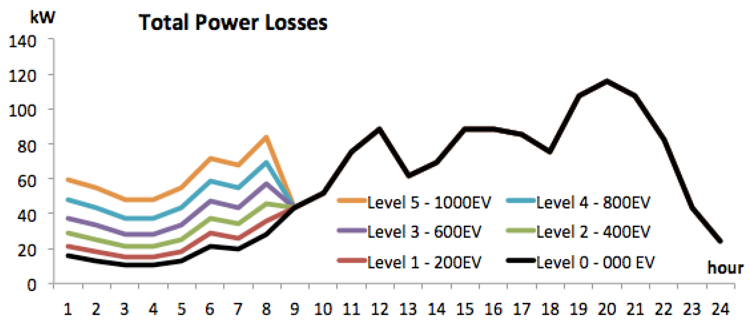
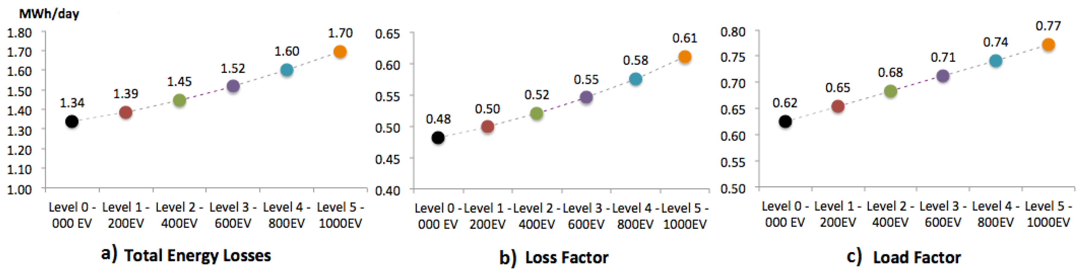
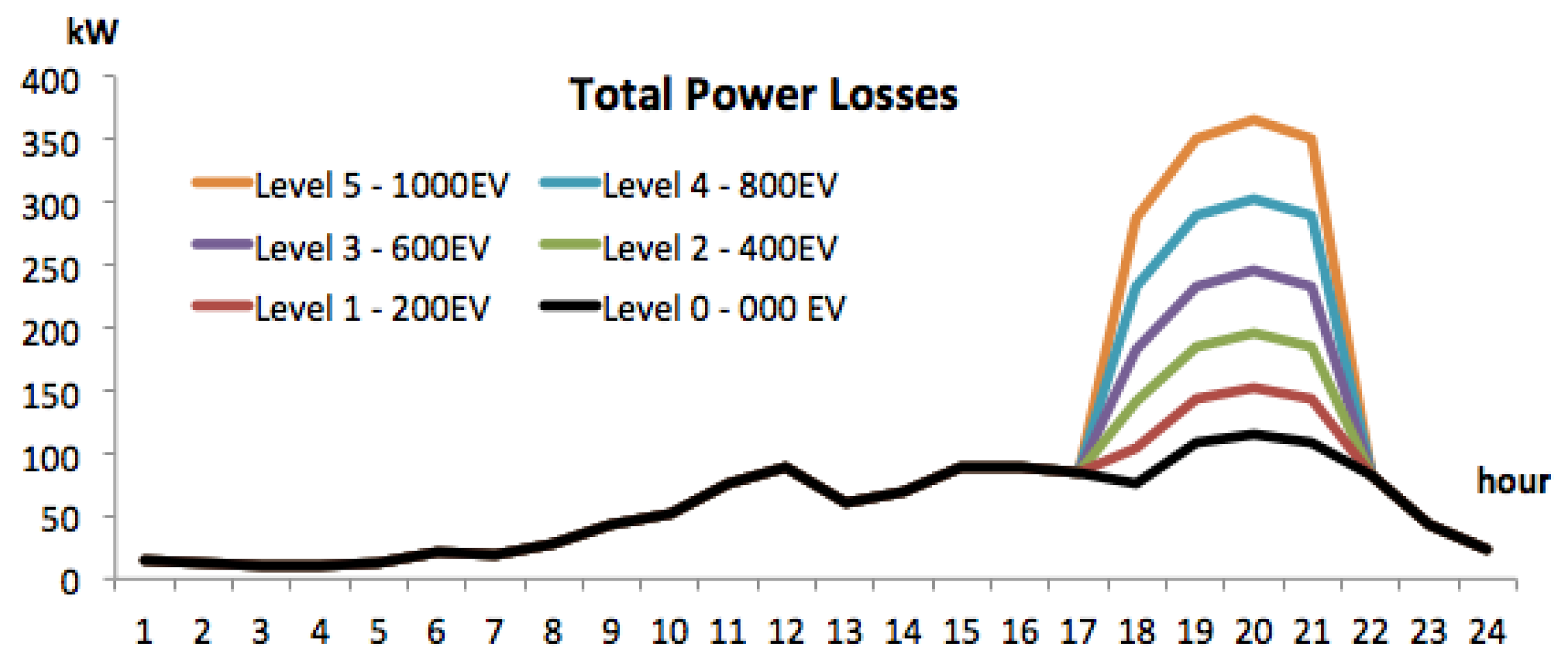
The 24-h power loss curves by each level for the connection of EV loads under off-peak conditions are depicted in Figure 3. Total real energy losses $\Delta W$ to be allocated among network users is evaluated by EV penetration level using Equation (9) and results are depicted in Figure 4. This figure also shows the resultant load and loss factor. Load and loss factors are defined as the ratio between average and maximum values of demands and losses, respectively.

Results reveal how the progressive integration of slow charging stations at off-peak load conditions produces a flattening effect of the load curve. The load factor increased from 0.62 at level 0 to 0.77. However, the loss factor also increased from 0.48 to 0.61. This means that 24-h power loss curve is also becoming flat. As result energy losses rose in magnitude from 1.24 MW·h/day, 1.05% (level 0) to 1.70 MW·h/day, 1.08% (level 5). This result is important since despite energy losses grew almost 50% in magnitude, the relative energy losses remains constant around 1.05–1.08%.

The absolute value of Marginal Loss Coefficients $\left|\right|ML{C}_{Di,t}^p\left|\right|$ are directly obtained for at each level k, each bus i, phase p and time t from fmincon results via Lagrange multipliers as indicated in Section 2.3.1.

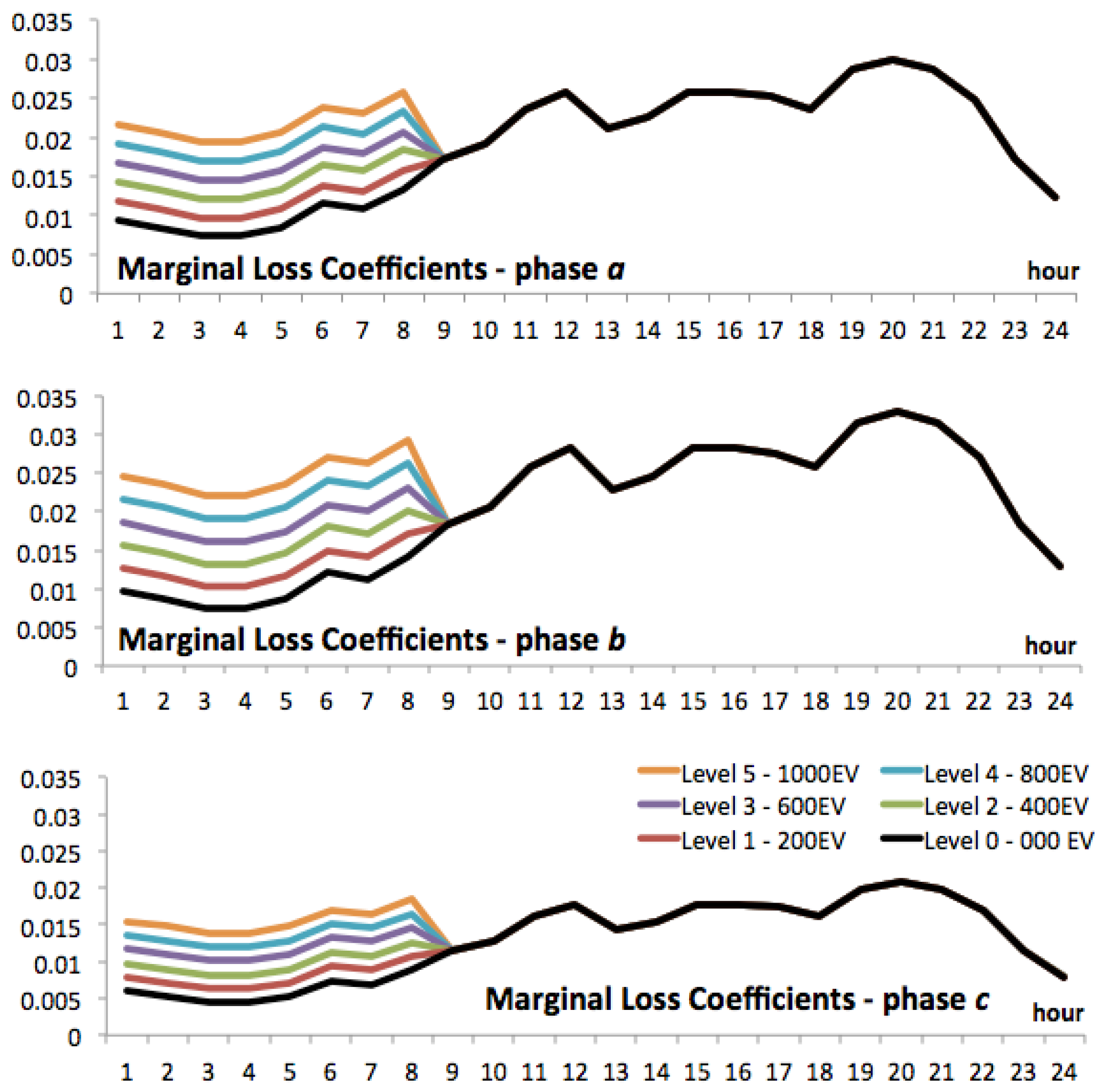
Figure 5 displays the MLCs curves when EVs are charging at off-peak time. The MLCs are applied to agents connected at bus 21 along 24 h. Note that under lower EV penetration (5%, red curve), MLCs observed between 01:00 and 09:00 are significantly lower than ones achieved between 10:00 and 22:00. For a high EV penetration (25%, orange curve), the MLCs obtained between 01:00 and 09:00 are similar to those achieved between 10:00 and 22:00 when no EV is connected (around 0.02–0.03 along the day). Then, under EV charging at off-peak load conditions, the pattern of MLCs is somehow flat, similar to a uniform marginal coefficient. This uniform coefficient produces similar results of a roll-in embedded method applied to recover the power losses.

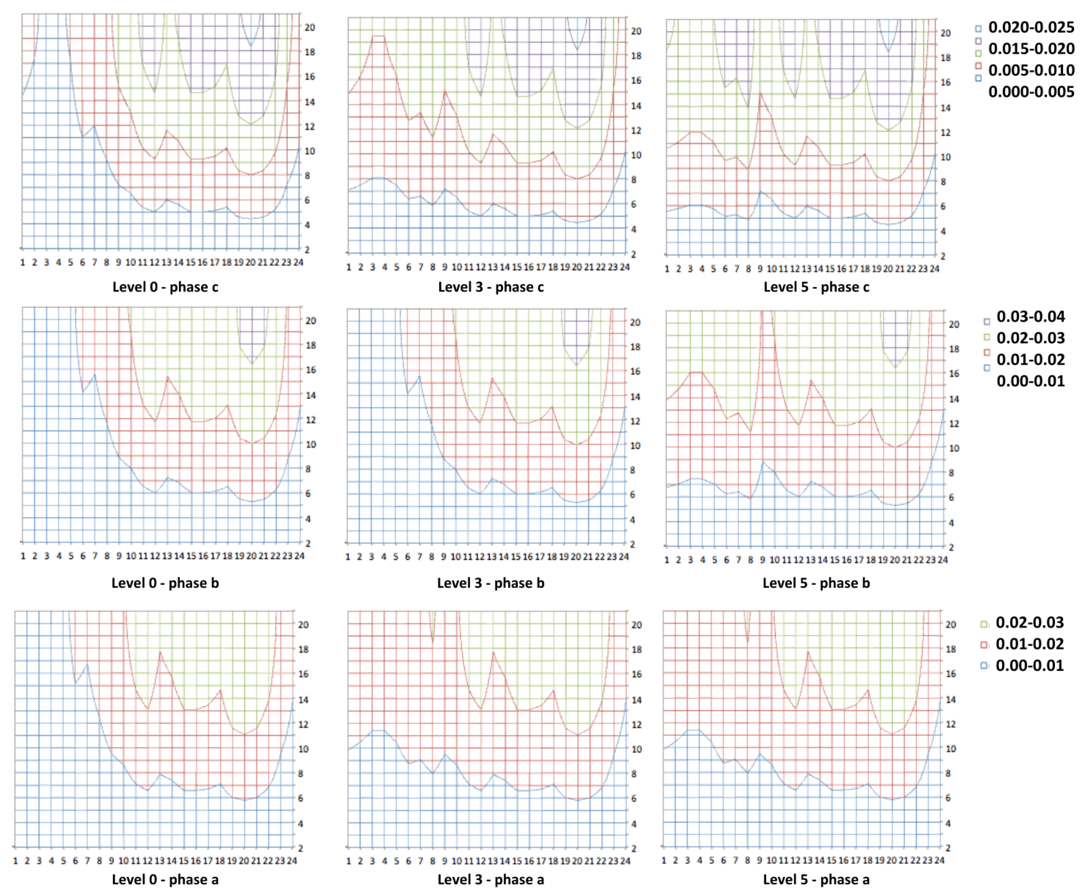
Figure 6 depicts a complete pattern for calculated MLCs by location and by time for each penetration level. It is worth to note in all phases that MLCs associated to high EV penetration (Level 5, 25%) cover more area (in time and location) than MLCs produced by lower levels.

Table 3. Off-peak load scenario: total energy losses allocated to PQ and EV loads by EV penetration level (kW·h/day).

Level	Pro Rata		Marginal		Energy Losses
	${\mathit{A}}_{\mathit{D}}^{\mathit{P},\mathit{PQ}}$	${\mathit{A}}_{\mathit{D}}^{\mathit{P},\mathit{EV}}$	${\mathit{A}}_{\mathit{D}}^{\mathit{M},\mathit{PQ}}$	${\mathit{A}}_{\mathit{D}}^{\mathit{M},\mathit{EV}}$	$\Delta \mathit{W}$
Level 0	1339.08, 100%	0.00, 0%	1339.08, 100%	0.00 0,%	1339.08
Level 1	1324.41, 96%	61.93, 4%	1352.52, 98%	33.82, 2%	1386.34
Level 2	1321.66, 91%	124.55, 9%	1363.84, 94%	82.37, 6%	1446.21
Level 3	1329.09, 88%	187.43, 12%	1373.19, 91%	143.32, 9%	1516.51
Level 4	1347.19, 84%	253.33, 16%	1381.59, 86%	218.93, 14%	1600.52
Level 5	1372.92, 81%	323.72, 19%	1389.30, 82%	307.33, 18%	1696.64

lists the general results for the allocated energy losses for aggregate PQ and EV loads under off-peak condition. The reconciliation factor $k_r$ was around 0.5 in all levels. Equations (18) and (28) were applied for the marginal and pro rata procedure, respectively. Energy losses range from 1339.08 kW·h/day at level 0 to 1696.64 kW·h/day at Level 5. At level 0, EVs do not exist then all losses are assigned to PQ loads. Regarding the allocation results, three facts can be highlighted:

EV charging stations operating under off-peak conditions and marginal loss allocation do not pay for additional energy losses. The marginal procedure assigns lower losses to EV than expected under a pro-rata procedure. This means that EV loads reach a small benefit by their produced losses at off-peak conditions. In fact, PQ loads do no take advantage of the marginal procedure being slightly penalized (they should pay for 1389 kW·h/day with respect to 1372 kW·h/day under the proportional approach).

Pro rata and marginal methods can produce a similar output when EV charging stations are operating under off-peak conditions. The share of energy losses attributable to EV loads (18%) are similar in both approaches: marginal and pro rata. This means that the MLCs are acting as a uniform factor capable to recover the cost of losses.

The EV share of losses is lesser than the EV share of consumption. For instance, at level 5 the ratio between EV and PQ loads consumption is 25%. The EV share of losses is lesser, 18%.

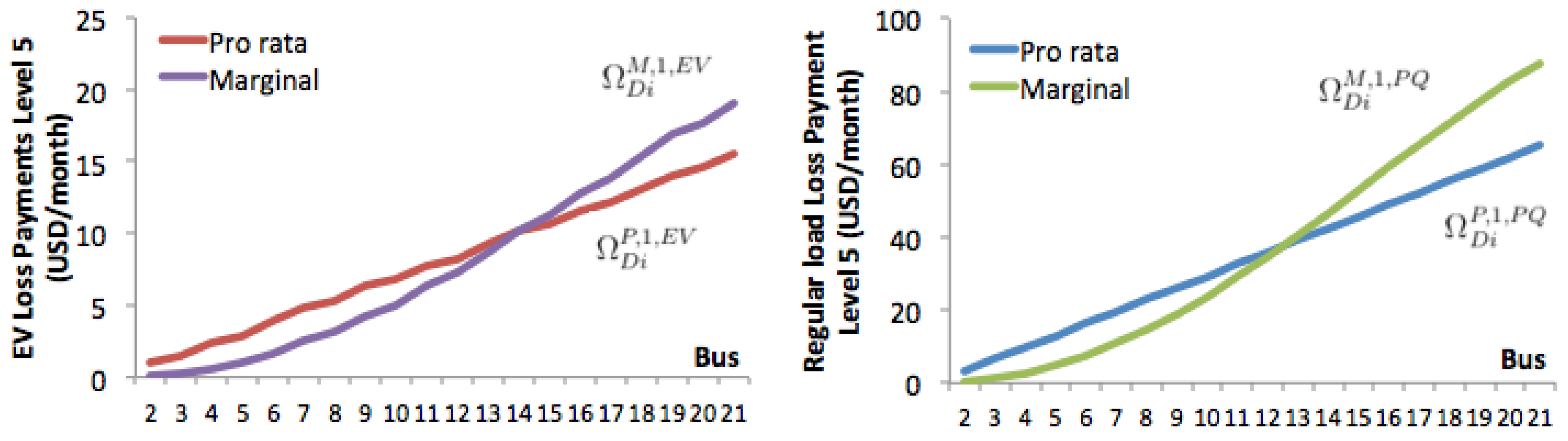
Payment for energy losses by EV location are calculated in a monthly basis using Equations (19) and (29) for marginal and pro rata procedure, respectively. Considering a flat energy price $\rho$ of 0.05 USD/kW·h, left-hand chart of Figure 7 shows how the marginal procedure penalize the slow EV charging stations connected from bus 15 to bus 21. A similar effect is also seen in PQ loads (right-hand chart of Figure 7) connected from bus 15 to bus 21. In this scenario, marginal procedure is applying higher charges to loads (EV and PQ) connected at the end of the line. Figure 7 also indicates that the application of MLCs for loads (EV and PQ) connected near to the origin have a lesser responsibility in the coverage of the entire energy losses.

4.2. Scenario 2: Fast Charging at Peak Load Conditions

In this scenario, EV connection was implemented at peak load conditions: from 18:00 to 21:00 with a 7.5 kW charging station considering the same five levels of integration applied in the case of EV charging at peak load conditions (Scenario 1), that is 200, 400, 600, 800 and 1000 units until reach a penetration of 25% of base energy consumption along one day.

The 24-h power loss curves by each level for the connection of EV loads under peak conditions are depicted in Figure 8. It is clear that the load curve becomes more sharp due to the progressive incorporation of slow EV charging stations.

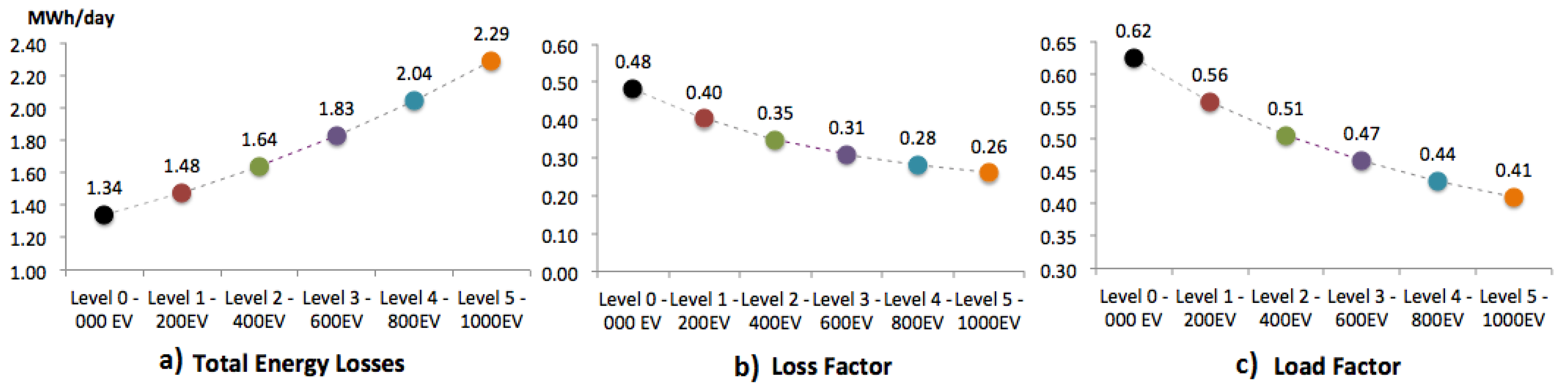
Total real energy losses $\Delta W$ to be allocated for each level among network users are indicated in Figure 9. Unlike Scenario 1, results show how the progressive integration of fast charging stations at peak load conditions produces a significative distortion effect of the load curve. EVs are charging only from 17:00 to 22:00. Then, the load factor decreased from 0.62 at Level 0 to 0.42 at Level 5. In this case, average demand does not grow in the same extent than the maximum value. As a result, the load factor falls. The loss factor also fall from 0.48 to 0.26 at Level 5. This means that energy losses drastically rose in magnitude from 1.24 MW·h/day, 1.05% (Level 0) to 2.30 MW·h/day, 1.8% (level 5). In this circumstance, the effects of EV charging stations at peak load condition are too harsh.

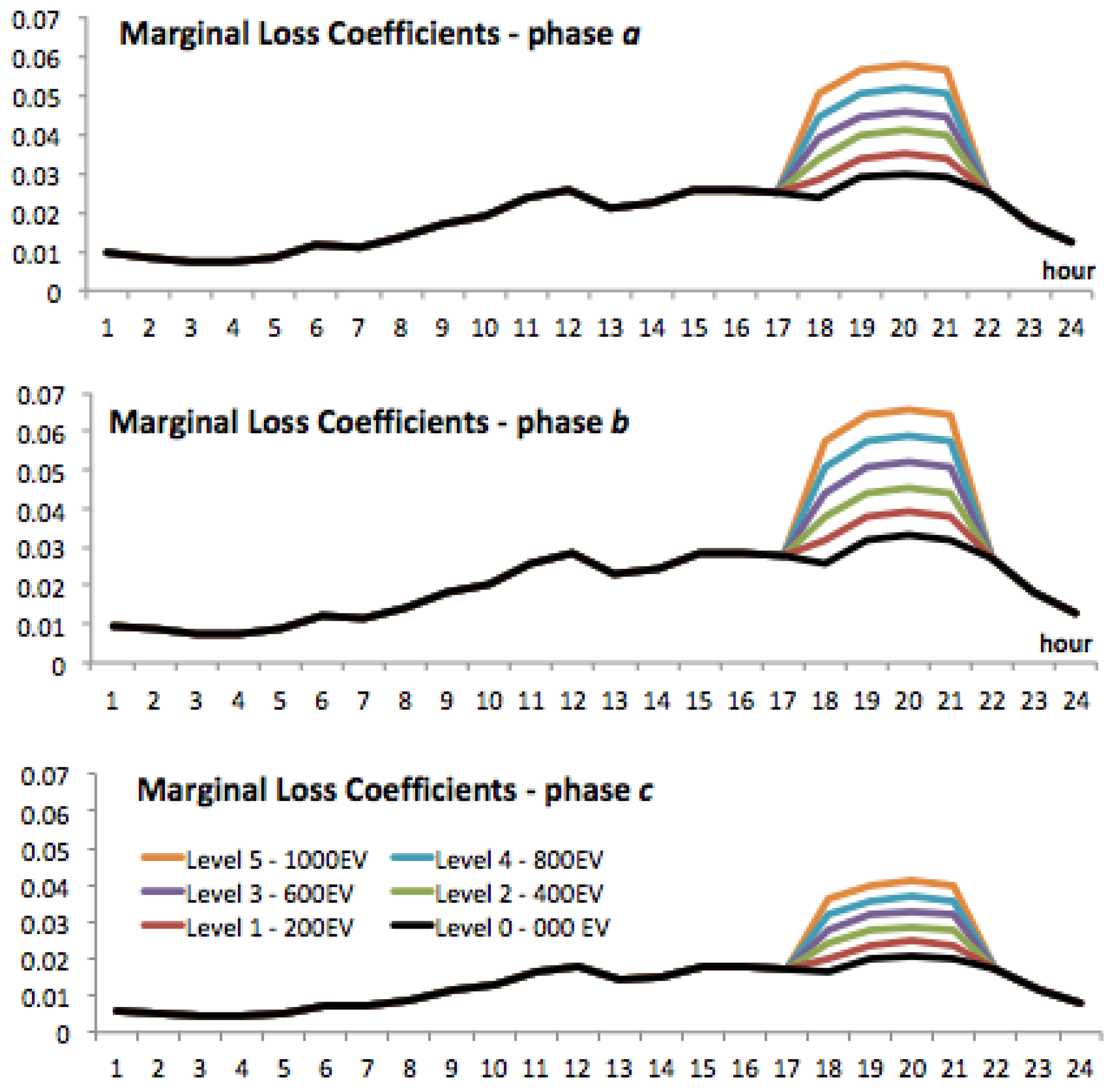
In Figure 10, the MLCs curves by EV penetration level at bus 21 along 24-h period is presented for the peak load conditions. It should be noted how marginal coefficients are able to reach high values 0.07 at peak time (18:00 and 21:00).

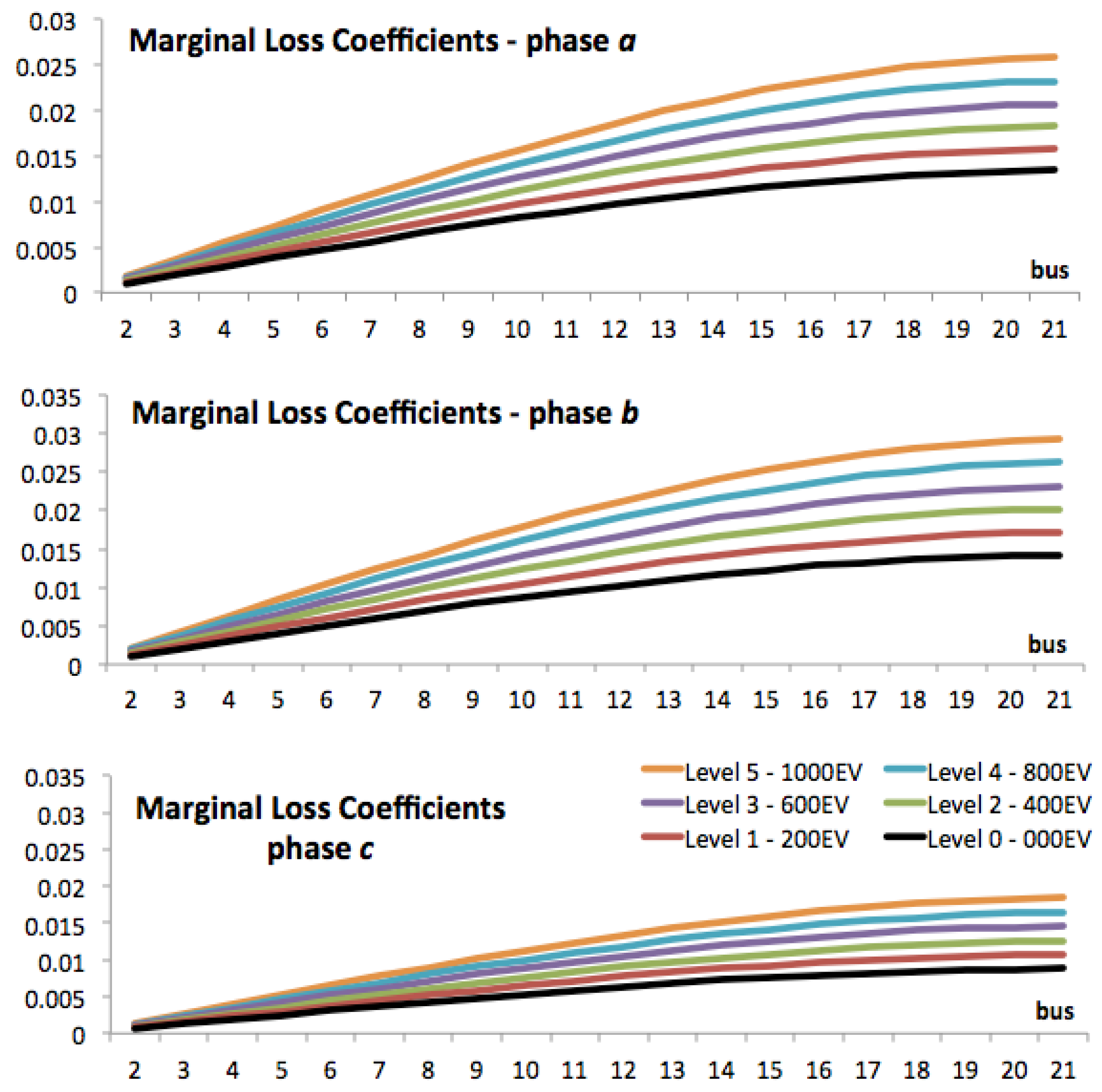
Figure 11 displays the MLCs curves when EVs are charging at 20:00. The MLCs are applied to agents connected from bus 2 to bus 21. As the load is increasing with the distance, the MLC magnitude at each bus also grows with the distance with respect to the reference bus. Then, closer loads to reference produce lower losses (and lower MLCs) than farther loads and therefore loads connected near to substation pay less for power losses than farthest loads.

In

Table 4. Peak load scenario: total losses allocated to PQ and EV loads (kW·h/day).

Level	Pro Rata		Marginal		Energy Losses
	${\mathit{A}}_{\mathit{D}}^{\mathit{P},\mathit{PQ}}$	${\mathit{A}}_{\mathit{D}}^{\mathit{P},\mathit{EV}}$	${\mathit{A}}_{\mathit{D}}^{\mathit{M},\mathit{PQ}}$	${\mathit{A}}_{\mathit{D}}^{\mathit{M},\mathit{EV}}$	$\Delta \mathit{W}$
Level 0	1339.08, 100%	0.00, 0%	1339.08, 100%	0.00, 0%	1339.08
Level 1	1410.22, 96%	66.03, 4%	1382.69, 94%	93.57, 6%	1476.26
Level 2	1499.45, 91%	141.52, 9%	1426.40, 87%	214.56, 13%	1640.96
Level 3	1601.37, 88%	226.19, 12%	1469.93, 80%	357.63, 20%	1827.56
Level 4	1720.74, 84%	324.16, 16%	1516.01, 74%	528.89, 26%	2044.90
Level 5	1851.48, 81%	437.40, 19%	1563.97, 68%	724.91, 32%	2288.88

, the energy allocation results for aggregate PQ and EV loads are presented for the peak load condition. The reconciliation factor $k_r$ also fluctuates around 0.5 in all levels. Equations (18) and (28) were applied for the marginal and pro rata procedure, respectively.

Unlike Scenario 1 where aggregate EV loads collect some marginal benefits due to the flattering effect over the load curve, Scenario 2 displays severe charges against EV loads due to energy losses associated with fast charging at peak conditions in all levels. If the marginal procedure is applied, PQ load should assume only a small part of the additional losses (23%). At Level 5, additional loses are 949 kW·h/day and PQ loads have to pay for 224 = 1563−1339 kW·h/day. Otherwise, if the pro rata procedure is applied, PQ loads should cover 46% of the incremental loads observed between Level 0 and Level 5.

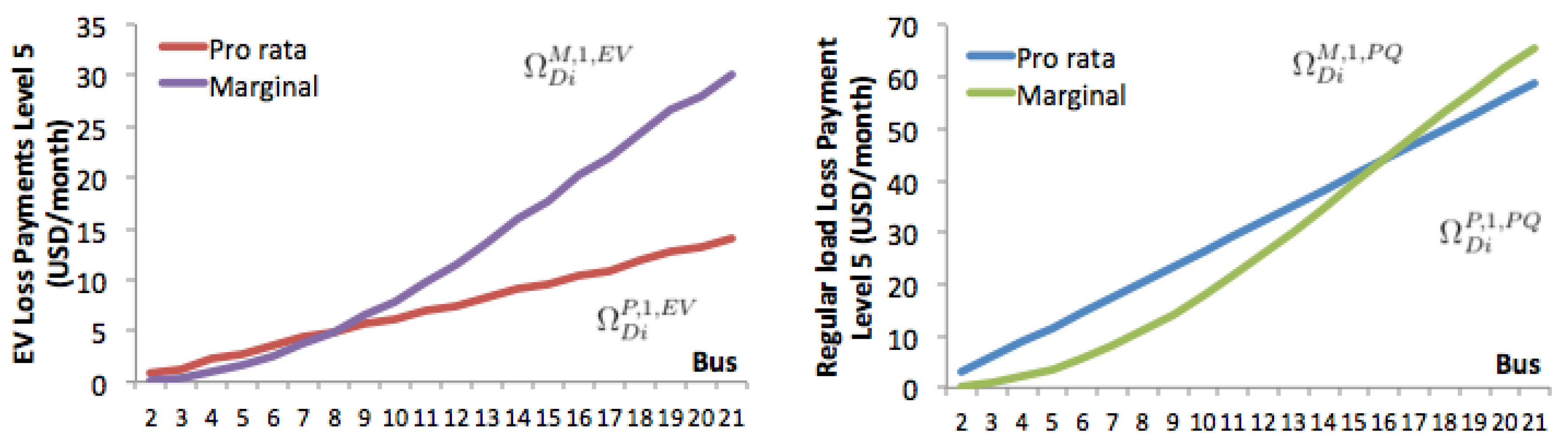
At Scenario 1 (EVs are charging at peak load conditions) pro rata and marginal allocation results lead to similar pattern. However, at Scenario 2 (EVs are charging at peak load conditions) marginal and pro rata loss allocation produce dissimilar results. EVs must pay for additional energy losses. The marginal procedure assigns higher losses to EV than calculated by the pro-rata procedure. This means that EV loads are duly charged by their produced losses at peak conditions. In this case, PQ loads take advantage of the marginal procedure since they have not to pay for additional losses. The share of energy losses attributable to EV loads under marginal approach (32%) is significantly higher than the share obtained by the pro rata procedure (19%). If we consider a flat energy price $\rho$ of 0.05 USD/kW·h, the left-hand chart of Figure 12 shows how the marginal procedure strongly penalize EVs connected from the middle to the end of the circuit. Note how EVs connected from bus 9 to bus 21 are facing high charges due to increasing losses. Conversely, the right-hand chart of Figure 12 visualizes how the marginal and pro rata procedures yield in similar charges. This means that there is not significative economical difference for PQ charges but strong incentives to EV loads to perform power loss reduction tasks.

4.3. The Economical Effects in a Single EV Unit Under Off-Peak and Peak Load Conditions

Consider now the perspective of a single EV of 30kW·h capacity when Level 5 is reached (25% of penetration). If a fixed energy price $\rho$ of 0.05 USD/kW·h is considered, the overall charging or energy cost for the EV is 1.5 USD/day. At off-peak and peak conditions, the connection of a single EV unit has different outcomes.

On the one hand, under off-peak load conditions (slow charging from 01:00 to 09:00), when the EV is connected at bus 21, phase 1 (ending node) the payment for losses under marginal procedure is almost 0.43 USD/day. This amount corresponds to 29% of total payment for energy (1.5 USD/day). On the other hand, under peak load conditions (fast charging from 19:00 to 21:00) the payment for losses under marginal procedure is 0.64 USD/day (54% of total payment for energy). This result is important since the best economic solution for the EV is charging under off-peak conditions.

Consider now that the EV is connected at bus 2, phase 1 (very close to substation). In this case, both scenarios show the same result, the EV has to pay only 0.03 USD/day (2% of total payment for energy). This charge is very low when compared with charges applied to loads at the end of the feeder. Then, the incentive is to connect EVs as close as possible to substation since no additional losses are produced.

Economic results for the marginal allocation procedure evidence EV loads connected at farthest loads have to pay important shares due to incremental losses becoming an important incentive (mainly at peak conditions) to provide network support. Under standard pro rata approach, the overall cost is distributed among all loads in a proportional manner and no incentive is provided by time of use and location of the EV charger.

4.4. The Impact of the EV Load Modeling on Loss Allocation Results

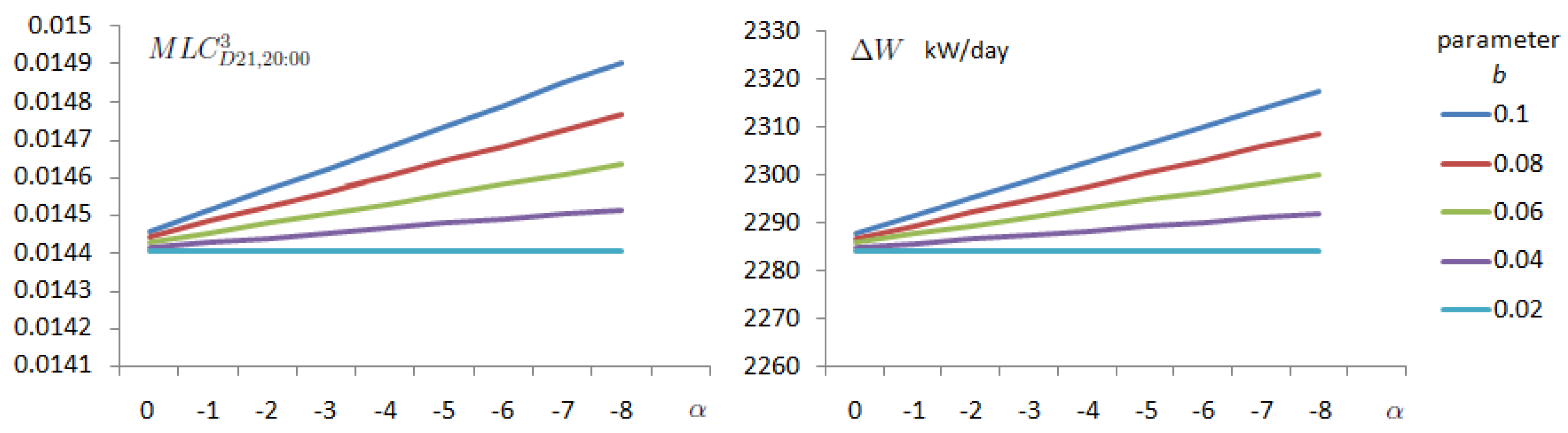
All results presented above were obtained assuming a specific EV load parametrization: a = 0.9537, b = 0.0463, and $\alpha$ = −2.324 in Equation (3). To evaluate the effects of the EV load model in the results, we ran the model under peak loading conditions (Level 5) varying $\alpha$ from 0 (PQ load) to −8.0 and b from 0.0 (PQ load) to 0.10. Results of the sensitivity analysis are depicted in Figure 13.

If the EV load is regarded as constant PQ ($\alpha$ = 0, b = 0.0), the marginal loss factor at 20:00, bus 21, Phase 3 ($ML{C}_{D21,20:00}^3$) is 0.014401769 and total losses to be allocated $\Delta W$ is 2284.12 kWh/day. Conversely, if the EV parameters take a non-linear form $\alpha$ = −8.0, b = 0.1, the marginal loss factor at 20:00, bus 21, Phase 3 ($ML{C}_{D21,20:00}^3$) is 0.014904362 and total losses to be allocated $\Delta W$ increased 2317.50 kW·h/day. These variations on MLCs and energy losses represent 3.5% and 1.5% of the values achieved when loads were assumed as PQ constant, respectively. As a result, we observe significant differences on loss factors and overall energy losses to be allocated among the network users. The adoption of a correct EV load model for economic evaluation of the impacts on losses becomes an important issue to consider to guarantee the fairness of the allocation procedure. As there are several charging protocols of EV batteries [37], future research on economical impacts of EVs on system losses should be devoted to include more detailed models.

5. Conclusions

This paper presents three-phase loss allocation procedure for distribution networks considering widespread connection of non-linear electric vehicle loads. The method was based on the computation of specific marginal loss coefficients (MLCs) per bus and phase. The method was applied in an illustrative unbalanced 12.47 kV feeder with 12,780 residential customers supposing different levels of EV penetration. Two operational cases with two different type of charging stations were considered. Results obtained were also compared with a traditional roll-in embedded method (pro rata).

Depending on the operational scheme adopted, two different situations deserve mention. Firstly, slow EV charging under off-peak demand conditions helps to flatten the load curve yielding moderate MLCs similar to those obtained by means of the pro rata procedure. Secondly, fast EV charging under peak conditions leads to a sharpened load curve with increasing losses and volatile MLCs for EV agents. In this case, marginal loss prices may become a strong incentive to optimize distribution system operation.

Sensitivity analysis results show the influence of the non-linear EV load model in the energy losses allocated. This result highlights the importance of considering an appropriate EV load model to appraise the overall losses to be allocated.

References

- Rotering, N.; Ilic, M. Optimal charge control of plug-in hybrid electric vehicles in deregulated electricity markets. IEEE Trans. Power Syst. 2011, 26, 1021–1029. [Google Scholar] [CrossRef]
- Deb, S.; Tammi, K.; Kalita, K.; Mahanta, P. Impact of Electric Vehicle Charging Station Load on Distribution Network. Energies 2018, 11, 178. [Google Scholar] [CrossRef]
- Bessa, R.J.; Matos, M.A. Economic and technical management of an aggregation agent for electric vehicles: A literature survey. Int. Trans. Electr. Energy Syst. 2012, 22, 334–350. [Google Scholar] [CrossRef]
- Zhang, Z.J.; Nair, N.C. Economic and pricing signals in electricity distribution systems: A bibliographic survey. In Proceedings of the IEEE International Conference on Power System Technology (POWERCON), Auckland, New Zealand, 30 October–2 November 2012; pp. 1–6. [Google Scholar]
- Pan, J.; Teklu, Y.; Rahman, S.; Jun, K. Review of usage-based transmission cost allocation methods under open access. IEEE Trans. Power Syst. 2000, 15, 1218–1224. [Google Scholar]
- Carpaneto, E.; Chicco, G.; Akilimali, J.S. Characterization of the loss allocation techniques for radial systems with distributed generation. Electr. Power Syst. Res. 2008, 78, 1396–1406. [Google Scholar] [CrossRef]
- Costa, P.M.; Matos, M.A. Loss allocation in distribution networks with embedded generation. IEEE Trans. Power Syst. 2004, 19, 384–389. [Google Scholar] [CrossRef]
- Bialek, J. Tracing the flow of electricity. IEE Proc. Gener. Transm. Distrib. 1996, 143, 313–320. [Google Scholar] [CrossRef]
- Galiana, F.D.; Conejo, A.J.; Kockar, I. Incremental transmission loss allocation under pool dispatch. IEEE Trans. Power Syst. 2002, 17, 26–33. [Google Scholar] [CrossRef]
- Weckx, S.; Driesen, J.; D’hulst, R. Optimal Real-Time Pricing for UnbalancedDistribution Grids with Network Constraints. In Proceedings of the IEEE Power and Energy SocietyGeneral Meeting (PESGM), Vancouver, BC, Canada, 21–25 July 2013. [Google Scholar]
- Heydt, G.T.; Chowdhury, B.H.; Crow, M.L.; Haughton, D.; Kiefer, B.D.; Meng, F.J.; Sathyanarayana, B.R. Pricing and control in the next generation power distribution system. IEEE Trans. Smart Grid 2012, 3, 907–914. [Google Scholar] [CrossRef]
- De Oliveira-De Jesus, P.M.; Castronuovo, E.D.; De Leao, M.P. Reactive power response of wind generators under an incremental network-loss allocation approach. IEEE Trans. Energy Convers. 2008, 23, 612–621. [Google Scholar] [CrossRef]
- Kaur, M.; Ghosh, S. Effective Loss Minimization and Allocation of Unbalanced Distribution Network. Energies 2017, 10, 1931. [Google Scholar] [CrossRef]
- Hong, M. An approximate method for loss sensitivity calculation in unbalanced distribution systems. IEEE Trans. Power Syst. 2014, 29, 1435–1436. [Google Scholar] [CrossRef]
- Li, R.Y.; Wu, Q.W.; Oren, S.S. Distribution locational marginal pricing for optimal electric vehicle charging management. IEEE Trans. Power Syst. 2014, 29, 203–211. [Google Scholar] [CrossRef]
- Kongjeen, Y.; Bhumkittipich, K. Impact of Plug-in Electric Vehicles Integrated into Power Distribution System Based on Voltage-Dependent Power Flow Analysis. Energies 2018, 11, 1571. [Google Scholar] [CrossRef]
- Shirmohammadi, D.; Gorenstin, B.; Pereira, M.V. Some fundamental, technical concepts about cost based transmission pricing. IEEE Trans. Power Syst. 1996, 11, 1002–1008. [Google Scholar] [CrossRef]
- Qian, K.; Zhou, C.; Allan, M.; Yuan, Y. Modeling of load demand due to EV battery charging in distribution systems. IEEE Trans. Power Syst. 2011, 26, 802–810. [Google Scholar] [CrossRef]
- Hernandez, J.C.; Ruiz-Rodriguez, F.J.; Jurado, F. Modelling and assessment of the combined technical impact of electric vehicles and photovoltaic generation in radial distribution systems. Energy 2017, 141, 316–332. [Google Scholar] [CrossRef]
- Kisacikoglu, M.C.; Ozpineci, B.; Tolbert, L.M. EV/PHEV bidirectional charger assessment for V2G reactive power operation. IEEE Trans. Power Electr. 2011, 28, 5717–5727. [Google Scholar] [CrossRef]
- Dharmakeerthi, C.H.; Mithulananthan, N.; Saha, T.K. Impact of electric vehicle fast charging on power system voltage stability. Int. J. Electr. Power Energy Syst. 2014, 57, 241–249. [Google Scholar] [CrossRef]
- Wasley, R.G.; Shlash, M.A. Newton-Raphson algorithm for 3-phase load flow. Proc. Inst. Electr. Eng. 1974, 121, 630–638. [Google Scholar] [CrossRef]
- Arrillaga, J.A.; Arnold, J.P. Computer Analysis of Power Systems; John Wiley & Sons, Inc.: Hoboken, NJ, USA, 1990. [Google Scholar]
- De Oliveira-De Jesus, P.M.; Alvarez, M.A.; Yusta, J.M. Distribution power flow method based on a real quasi-symmetric matrix. Electric. Power Syst. Res. 2013, 95, 148–159. [Google Scholar] [CrossRef]
- Montenegro, D.; Hernandez, M.; Ramos, G.A. Real time OpenDSS framework for distribution systems simulation and analysis. In Proceedings of the 2012 Sixth IEEE/PES Transmission and Distribution: Latin America Conference and Exposition (T&D-LA), Montevideo, Uruguay, 3–5 September 2012. [Google Scholar]
- Mutale, J.; Strbac, G.; Curcic, S.; Jenkins, N. Allocation of losses in distribution systems with embedded generation. IEE Proc. Gener. Transm. Distrib. 2000, 147, 7–14. [Google Scholar] [CrossRef]
- Stoft, S. Power System Economics; IEEE Press & Wiley-Interscience: Hoboken, NJ, USA, 2002. [Google Scholar]
- Kersting, W.H. A three-phase unbalanced line model with grounded neutrals through a resistance. In Proceedings of the 2008 IEEE Power and Energy Society General Meeting-PESGM, Pittsburgh, PA, USA, 20–24 July 2008; pp. 12651–21652. [Google Scholar]
- Gonen, T. Electric Power Distribution Engineering, 2nd ed.; CRC Press: Boca Raton, FL, USA, 2008. [Google Scholar]
- Dugan, R.C.; McDermott, T.E. An open source platform for collaborating on smart grid research. In Proceedings of the IEEE Power Energy Society General Meeting, Detroit, MI, USA, 24–29 July 2011; pp. 1–7. [Google Scholar]
- Mocci, S.; Natale, N.; Ruggeri, S.; Pilo, F. Multi-agent control system for increasing hosting capacity in active distribution networks with EV. In Proceedings of the IEEE International Energy Conference (ENERGYCON), Cavtat, Croatia, 13–16 May 2014; pp. 1409–1416. [Google Scholar]
- Kisacikoglu, M.C.; Erden, F.; Erdogan, N. Distributed control of PEV charging based on energy demand forecast. IEEE Trans. Ind. Inf. 2018, 14, 332–341. [Google Scholar] [CrossRef]
- Ruiz-Rodriguez, F.J.; Hernandez, J.C.; Jurado, F. Voltage behaviour in radial distribution systems under the uncertainties of photovoltaic systems and electric vehicle charging loads. Int. Trans. Electr. Energy Syst. 2018, 28, 2490. [Google Scholar] [CrossRef]
- Munkhammar, J.; Widen, J.; Ryden, J. On a probability distribution model combining household power consumption, electric vehicle home—Charging and photovoltaic power production. Appl. Energy 2015, 142, 135–143. [Google Scholar] [CrossRef]
- Ruiz-Rodriguez, F.J.; Hernandez, J.C.; Jurado, F. Probabilistic Load-Flow Analysis of Biomass-Fuelled Gas Engines with Electrical Vehicles in Distribution Systems. Energies 2017, 10, 1536. [Google Scholar] [CrossRef]
- ElNozahy, M.S.; Salama, M.M. A comprehensive study of the impacts of PHEVS on residential distribution networks. IEEE Trans. Sustain. Energy 2014, 5, 332–342. [Google Scholar] [CrossRef]
- Godina, R.; Paterakis, N.G.; Erdinc, O.; Rodrigues, E.M.G.; Catalão, J.P.S. Impact of EV charging-at-work on an industrial client distribution transformer in a Portuguese Island. In Proceedings of the 2015 Australasian Universities Power Engineering Conference (AUPEC), Wollongong, Australia, 27–30 September 2015; pp. 1–6. [Google Scholar]
Figure 1.
Three-phase distribution system with Electric Vehicles (EV) loads.
Figure 2.
Base load curve: No EV connected, only constant real and reactive power (PQ) loads.
Figure 3.
Off-peak load scenario: 24-h power losses by EV penetration level.
Figure 4.
Off-peak load scenario: energy losses, loss and load factors by EV penetration level: (a) total energy losses; (b) loss factor; (c) load factor.
Figure 5.
Off-peak load scenario: marginal loss coefficients (MLCs) at Bus 21 by EV penetration level and by time.
Figure 6.
Off-peak load scenario: MLCs pattern by node and by time (Levels 0, 3 and 5).
Figure 7.
Off-peak load scenario: economic allocation between PQ and EV users connected at Phase 1 (Level 5).
Figure 8.
Peak load scenario: 24-h power losses by EV penetration level.
Figure 9.
Peak load scenario: energy losses, loss and load factors by EV penetration level: (a) total energy losses; (b) loss factor; (c) load factor.
Figure 10.
Peak load scenario: MLCs at Bus 21 by EV penetration level and by time.
Figure 11.
Peak load scenario: MLCs at 20:00 by EV penetration level and by bus.
Figure 12.
Peak load scenario: economic allocation between PQ and EV users connected at phase 1 (Level 5).
Figure 13.
Sensitivity analysis: MLCs and total losses against EV parameters and b.