Ensemble Recurrent Neural Network Based Probabilistic Wind Speed Forecasting Approach

Abstract

Wind energy is a commonly utilized renewable energy source, due to its merits of extensive distribution and rich reserves. However, as wind speed fluctuates violently and uncertainly at all times, wind power integration may affect the security and stability of power system. In this study, we propose an ensemble model for probabilistic wind speed forecasting. It consists of wavelet threshold denoising (WTD), recurrent neural network (RNN) and adaptive neuro fuzzy inference system (ANFIS). Firstly, WTD smooths the wind speed series in order to better capture its variation trend. Secondly, RNNs with different architectures are trained on the denoising datasets, operating as sub-models for point wind speed forecasting. Thirdly, ANFIS is innovatively established as the top layer of the entire ensemble model to compute the final point prediction result, in order to take full advantages of a limited number of deep-learning-based sub-models. Lastly, variances are obtained from sub-models and then prediction intervals of probabilistic forecasting can be calculated, where the variances inventively consist of modeling and forecasting uncertainties. The proposed ensemble model is established and verified on less than one-hour-ahead ultra-short-term wind speed forecasting. We compare it with other soft computing models. The results indicate the feasibility and superiority of the proposed model in both point and probabilistic wind speed forecasting.

1. Introduction

The demand of renewable energy application is growing stronger over the recent years, in response to increasingly high energy consumption and serious environment pollutions [1]. The global renewable energy capacity has exceeded 1800 GW by the end of 2015 [2,3]. Among those energy sources, wind power is a typical kind, which is widely distributed and easy to access and it has become one of the fastest developing sources. Nevertheless, the chaotic nature of wind speed is unavoidable, which restricts the application of in-grid wind power. As wind fluctuates arbitrarily and uncertainly, wind power integration will challenge the security and stability of power system operations. Therefore, an accurate wind speed forecasting is expected for the development of large-scale wind power utilization, which can benefit wind power integrated system.

There are customarily three major methodologies for wind energy forecasting, that is, physical, statistical and soft computing methodologies [4,5,6]. Firstly, physical models are established based on numerous physical variables, including geographical and meteorological factors. As the formation of wind is influenced by many elements, for example, surface temperature and sunshine duration, physical models specialize in long-term forecasting and trend forecasting [7,8]. However, physical methodologies usually take a great deal of computation time due to the large number of inputs and their accuracies depend on the results from numerical weather prediction (NWP). Secondly, statistical models are aimed at developing relationships between the historical (input) and future (output) wind energy data. Auto regressive moving average (ARMA), auto regressive integrated moving average (ARIMA) and their hybrid models are most frequently utilized in statistical prediction methodologies [9,10,11,12]. Lastly, soft computing methodologies are most widely used in renewable energy forecasting [13]. Among those methods, artificial neural network (ANN) is a typical soft computing model. In Reference [14,15,16], polynomial ANN, radial basis function (RBF) ANN and physical hybrid (PH) ANN are introduced for wind and solar energy forecasting. Besides, there are massive other forecasting models proved efficient in literatures. In Reference [17,18,19], support vector machine (SVM) is introduced to achieve better wind power forecasting results when the number of training samples are limited. Extreme learning machine (ELM) is a recently proposed model that has a high training speed and is suitable for ultra-short online forecasting [20,21,22]. Adaptive neuro-fuzzy inference system (ANFIS) is a simpler model than ANN while can also approximate any non-linear function, which is proven feasible in wind speed forecasting [23]. Nevertheless, those models have limited generalization performance and can be hardly trained on a large amount of training data.

As a result, deep learning theory has been developed in order to overcome the shallow learning abilities of traditional soft computing methods. As they can be trained on a large number of samples, they are ideally suitable for big data analysis and have emerged their superiorities in the field of renewable energy forecasting. Stacked auto-encoder (SAE) and deep belief network (DBN) are two models that solve the optimization problem in deep multi-layer perceptron (MLP), which have successfully been applied in wind speed and power forecasting [24,25,26]. In Reference [27], deep convolutional neural network (CNN) is introduced to predict wind power using two-dimensional inputs. Besides, recurrent neural network (RNN) is also a new deep-learning-based model, which holds the ability to learn temporal correlations in a complete sequence. It has also been introduced to point wind speed forecasting [28,29]. Hence, RNN is chosen as the sub-model in this study for probabilistic wind speed forecasting and it will be compared with other soft computing methods.

Moreover, in order to combine the advantages of different models, extensive hybrid forecasting models have been proposed. In addition to pre-processing and post-processing, the ensemble of sub-models is an efficient approach [30], which is also called competitive ensemble forecasting [31]. The final forecasting result is usually calculated via an averaging or weighting procedure [32]. This method has two advantages: first, the prediction error of a sole model can be reduced through competitions in sub-models; second, a confidence level for probabilistic forecasting can be obtained based on the variance of those sub-models. In Reference [33], an ensemble model based on Gaussian process regression (GPR) and ANN possesses a superb precision in short-term wind power forecasting. In Reference [34], adaptive boosting (AdaBoost) is combined with ELM for multi-step-ahead wind speed forecasting. A wind power forecasting model mixed bagging and ANN is proposed in Reference [35]. Those models share a common characteristic that the number of sub-models is considerable. However, it costs a lot of computation time to train a sole deep-learning-based sub-model. In order to ensure the performance of ensemble with a small number of RNNs, an ANFIS model is built as the top layer of the ensemble forecasting model in this study. A combined result of those sub-models is achieved through the learnt fuzzy rules, rather than a simple weighting approach.

In this study, a hybrid ensemble model is proposed for short-term probabilistic wind speed forecasting, which consists of wavelet threshold denoising (WTD), RNN and ANFIS. The WTD is a pre-processing approach to decrease the fluctuations in wind speed datasets. RNN and ANFIS are utilized to build an ensemble probabilistic forecasting model. The main contributions of this study are listed as follows:

• The ANFIS model is innovatively established as the top layer of the ensemble model to calculate a better forecasting result rather than just an averaged value from sub-models.
• In order to maintain diversities of sub-models and take advantages of ensemble learning, different architectures are introduced to build RNNs, including long short-term memory (LSTM), gated recurrent unit (GRU) and dropout layer.
• The variances collected from sub-models are introduced to probabilistic forecasting problem, which inventively consist of two parts, namely modeling uncertainties and forecasting uncertainties.

We compare the proposed WTD-RNN-ANFIS model with several soft computing models in various point and probabilistic forecasting cases, in order to prove its feasibility and superiority. The rest of this paper is structured as follows. Section 2 introduces the utilized datasets, as well as detailed architecture and algorithms of the probabilistic forecasting model. Section 3 presents concise forecasting results based on the proposed approach. Section 4 contains the detailed discussion and comparisons in probabilistic forecasting performance. Finally, a conclusion is drawn in Section 5.

2. Materials and Methods

2.1. Datasets

The training and testing datasets utilized in this study are based on wind speed data measured in the interval of 15 min at the height of 50 m, which are collected by the wind tower of National Renewable Energy Laboratory (NREL) National Wind Technology Center (NWTC) [36]. The tower is located in the latitude of 39.91° N, the longitude of 105.23° W and the elevation of 1855 m. When the measured data is missing or incorrect due to equipment failure, it can be substituted by the mean value obtained from previous or subsequent points, or by the value calculated from intelligent imputation technologies for example, decision tree [37].

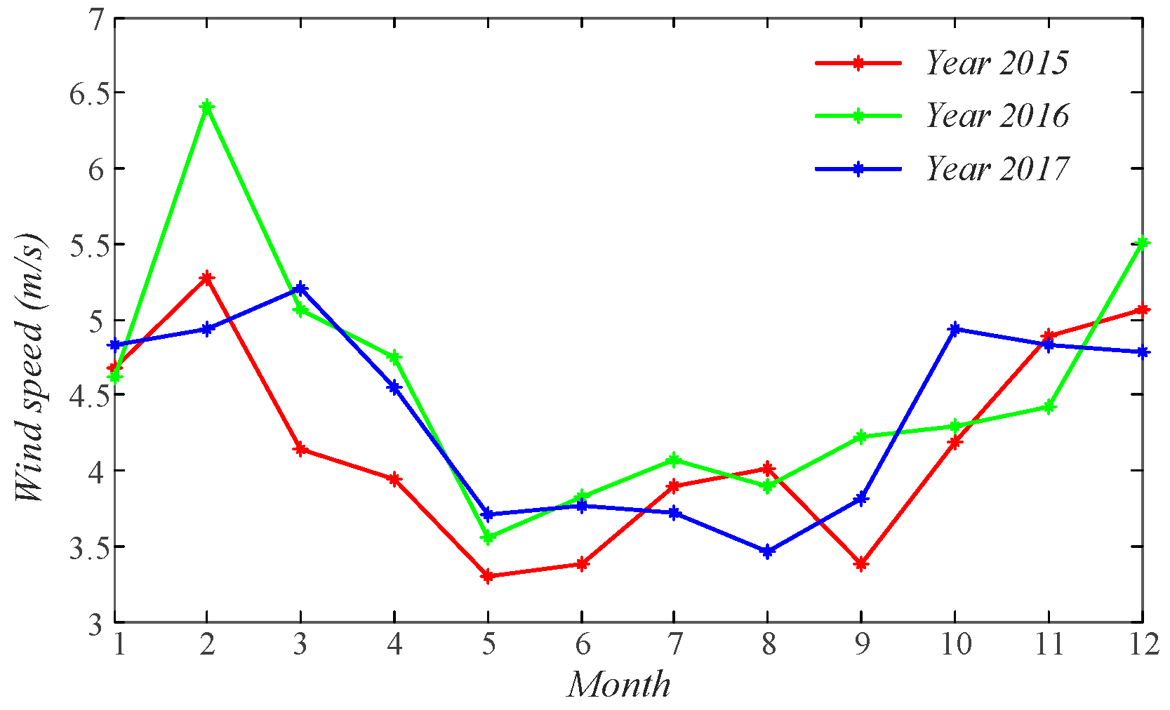
In Figure 1, the monthly averaged values of wind speed from 2015 to 2017 are exhibited, from which it can be found that wind speed varies under a certain seasonal regularity. The averaged values of wind speed in May, June, July and August are smaller than those in November, December, January and February. In this study, the wind speed datasets in 2015 and 2016 are used as training samples and those in 2017 are for the test phase. Specially, according to the above analysis, we choose four testing cases of different seasons. The wind speed data on 22 March 2017, 23 June 2017, 22 September 2017 and 23 December 2017 are chosen to be testing samples as representative dates of spring, summer, autumn and winter seasons, in order to fully validate and compare the performances of different forecasting models.

2.2. Architecture of the Entire Forecasting Model

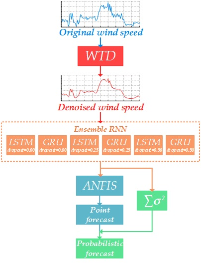
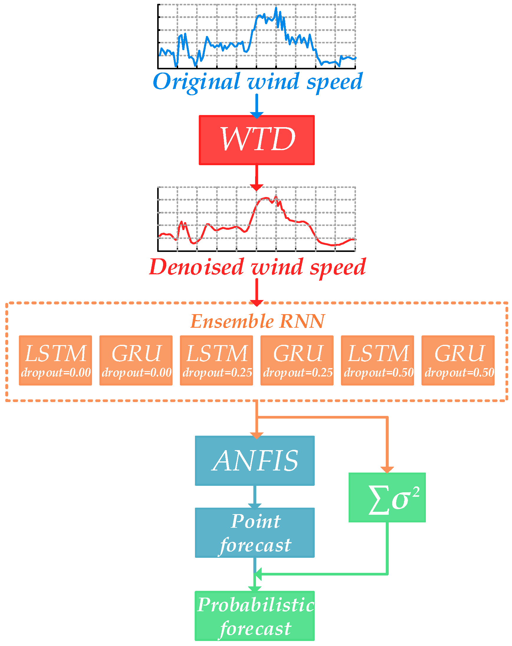
The probabilistic wind speed forecasting model proposed in this study consists of WTD, RNN and ANFIS. Firstly, WTD is used to decompose and smooth historical time series of wind speed in order to reduce its volatility. In that case, it is easier for a forecasting model to capture the variation trend of wind speed. Secondly, six RNNs with dissimilar architectures and parameters, namely sub-models, are established and trained for prediction. Thirdly, an ANFIS is utilized as the top layer of the ensemble model. The outputs of those RNNs are entered into the ANFIS and the final forecasting result is attained from its output. Finally, variances are gathered from different sub-models, along with errors between the final predicted value and the actual value, so prediction intervals of different confidence levels can be calculated. The structure of the entire WTD-RNN-ANFIS model is shown in Figure 2.

2.3. Wavelet Threshold Denoising (WTD)

WTD is based on wavelet transform (WT), which is a time-scale approach for signal processing. As WT holds the characteristics of local feature representation and multi-resolution analysis [38], it has been proved effective in dealing with non-stationary series and time varying problems [39,40]. A mother wavelet ϕ(t) is essential in WT. It can be scaled and time-shifted via scale factor a and shift factor b, producing a set of child wavelets to extract features under different resolutions. Moreover, WT includes two categories: continuous wavelet transform (CWT) and discrete wavelet transform (DWT). DWT has scale and shift factors in discrete forms, which reduces computation cost with little loss of signal information. It is especially suitable for sampled signals as well. The wavelet function of DWT is expressed as follows [41]:

$${\varphi }_{j,k}(t)=2^{-\frac{j}{2}}\varphi (2^{-j}t-k),$$

(1)

where j and k are integer-valued scale and shift factors, respectively; t represents the time variable; and ϕ(t) is the mother wavelet. The wavelet functions are binary wavelets and they are utilized to conduct DWT as [41]:

$$W_{j,k}(t)=2^{-\frac{j}{2}}{\displaystyle \sum _{t}x(t)}{\varphi }^{*}(2^{-j}t-k),$$

(2)

where ϕ^*(·) represents a convolution operation using wavelet function and x(t) is the sampled signal.

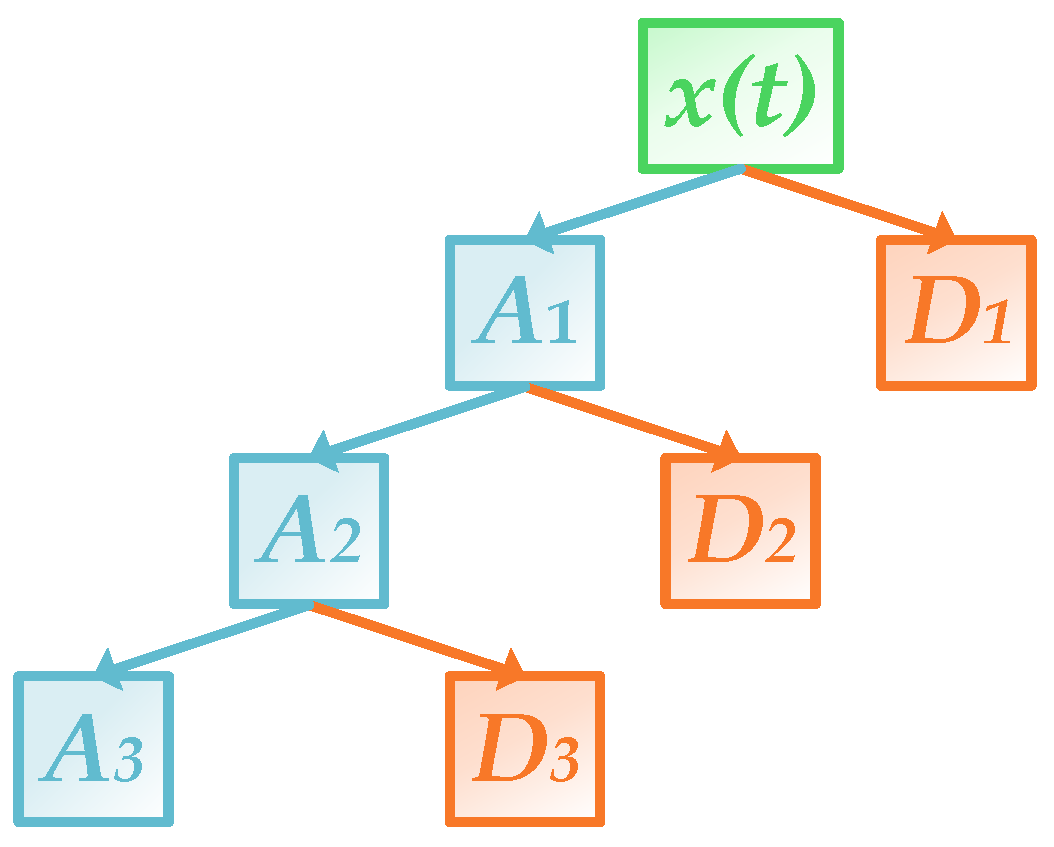
Mallat algorithm is commonly used for DWT, where scale functions and wavelet functions are operating as low and high pass filters, respectively. The multi-level decomposition of the algorithm is shown in Figure 3. After decomposition, approximation and detail components are obtained, which contain low-frequency and high-frequency information, respectively [41]:

$$x(t)={\displaystyle \sum _k{A}_{j,k}(t){\psi }_{j,k}(t)}+{\displaystyle \sum _j{\displaystyle \sum _k{D}_{j,k}(t){\varphi }_{j,k}(t)}},$$

(3)

where ψ_j,k and ϕ_j,k are the scale and wavelet functions, respectively; A_j,k is called the approximation component or scale coefficient and D_j,k is the detail component or wavelet coefficient. As the Gaussian white noise in a signal is discontinuous, its coefficients in wavelet domain, which are centered in detail components, also follow the Gaussian distribution. Therefore, coefficients of noise are smaller than those of the effective signal. In this case, WTD is able to utilize a certain threshold to extract the noise and sets its coefficients to be zero.

Based on the above explanations, the procedure of WTD for wind speed is simply summed up into three steps:

• Decompose the original time series of wind speed using WT;
• Calculate the threshold to distinguish the noise from the effective signal;
• Set the wavelet coefficients of noise to be zero and reconstruct the wind speed series.

It also should be mentioned that there are several parameters in WTD to be determined artificially: the wavelet basis function, the number of decomposition levels, threshold computation approach and denoising approach.

2.4. Recurrent Neural Network (RNN)

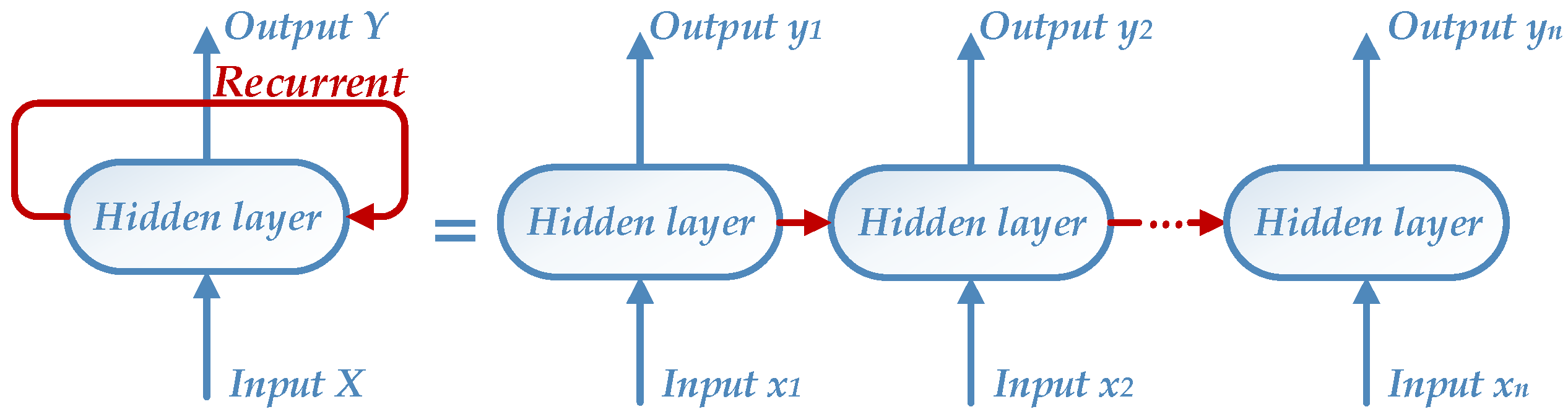
RNN has a strong power to handle a sequence with temporal correlation and it has been widely utilized in solving time-varying problems [42,43], especially natural language processing [44]. Unlike a common neural network that has no connections within hidden layers, RNN is able to connect hidden layers with the former ones circularly. Those hidden layers of RNN, which are also named recurrent units, can save historical information from the sequence. The sequential structure of a one-hidden-layer RNN is shown in Figure 4. It can be unfolded to several networks with hidden layers connected, each of which has a point input of a sequence. Therefore, a RNN possesses an extremely deep architecture, the number of whose hidden layers is equal to the length of input sequence.

In this study, RNNs are established and trained as sub-models for ensemble forecasting. In order to make full use of ensemble technology and enhance forecasting accuracy, it is of great significance to keeping diversities of sub-models. In order to deal with this issue, several approaches are considered and discussed as follows:

• Choose different datasets to train sub-models, for example, bagging technology. In bagging, a random sampling with replacement is operated for training datasets. Thus, datasets may contain duplicated samples or not [45]. However, a quite large number of sub-models is essential for this method, whereas it is expensive in terms of computation cost for deep-learning-based models.
• Set dissimilar parameters for sub-models, for example, the numbers of neural nodes and hidden layers in ANN. Nevertheless, it is hard in itself to set those parameters as they are often determined by trial and error of many times in practical application.
• Establish diverse models or models with different architectures, for example, different recurrent units in RNN.
• Adopt dropout technology in ANN. Dropout is a state-of-art method to regularize fixed-sized models and prevent them from over-fitting [46]. As model training has a certain randomness with dropout, diversities of sub-models are generated.

Accordingly, two recurrent architectures are utilized to build sub-models of RNNs in this study, namely LSTM and GRU. Dropout is used as well and it is in the form of layer structures in RNN.

2.4.1. Dropout Layer

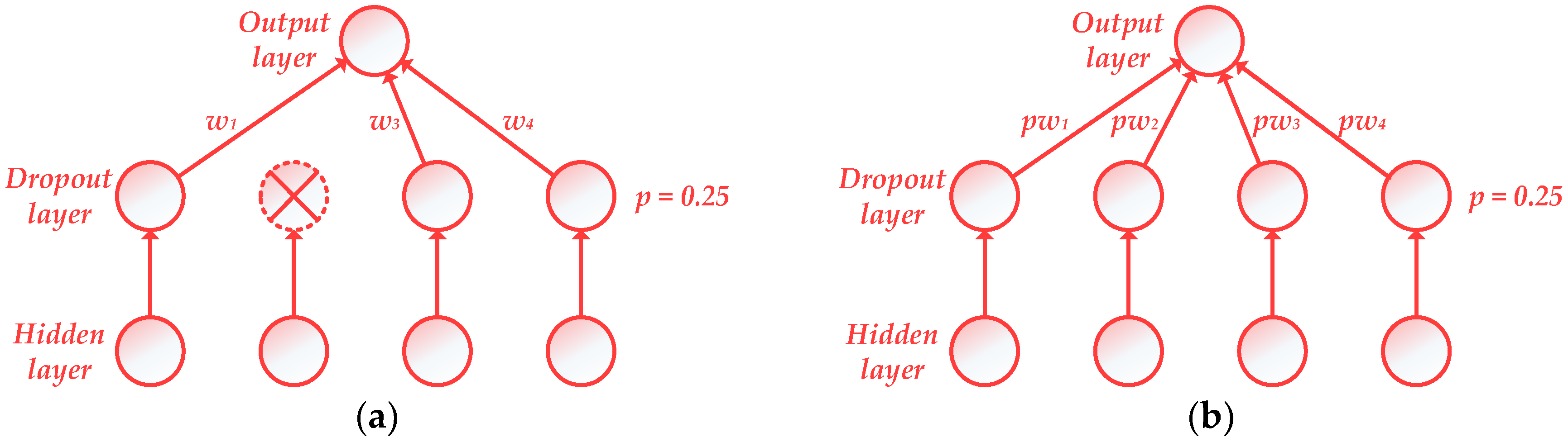
The structure of a dropout layer is shown in Figure 5. Several connections of neural nodes between two hidden layers are blocked with a certain dropout rate p in one iteration and those nodes are not able to participate in training [47].

During the training phase, a certain proportion (p) of the nodes are abandoned randomly, whose weights W are not updated. Therefore, different parts of an ANN are trained in different iterations. While the testing stage, a ‘thinner’ network is obtained, where all nodes are connected with the new weights pW.

2.4.2. LSTM

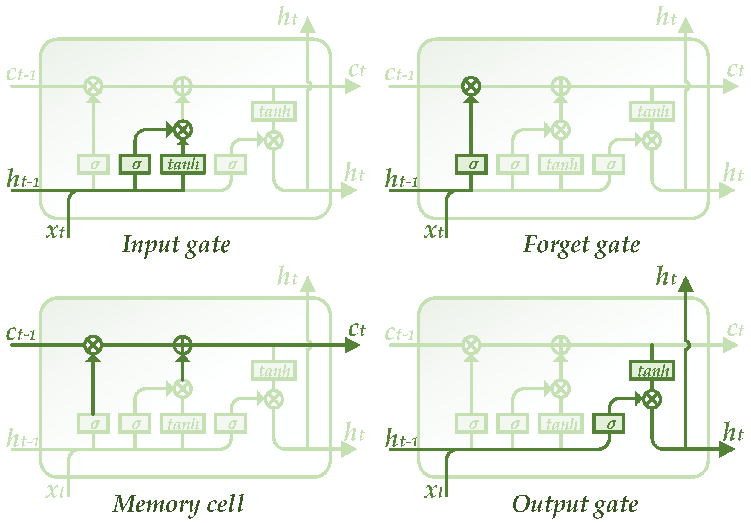
A simple RNN shown in Figure 4 has numerous connections between current and previous hidden layers. Thus, training such a network becomes quite difficult, where the vanishing gradient problem will arise. In order to overcome the problem, LSTM was proposed in 1997 [48,49] and has been improved during the recent rapid development of deep learning technology [50]. It is a building unit for layers of RNN, which is able to remember short-term memory that lasts for a long period of time. The structure of a LSTM block is presented in Figure 6, which consists of four major parts, namely input gate, forget gate, memory cell and output gate.

From the shown structure of LSTM, it is seen that two parallel lines are working to deal with the hidden layer information and memory, which is the most significant variance from a simple RNN. Hidden layer line h computes its output value based on the input and historical hidden information and its computation result is sent to both the next layer and memory line c. The memory line receives those results and forgets redundant ones, producing a modified output to affect hidden layer line. The realizations of the above functions are decided by these controllable gates with dissimilar architectures and equations [29]:

Input gate. It receives information from the previous hidden layer and the current input. Then it computes to obtain an output with the following equation:

$$i_t=\sigma (w_{xi}{x}_t+w_{hi}{h}_{t-1}+b_i),$$

(4)

where i_t is the output of input gate; x_t and h_t−1 are the current input and the previous hidden layer output, respectively; w_xi and w_hi are weights for inputs x_t and h_t−1, respectively; and b_i is the bias of the input gate. σ is the activation function and a soft sign function is adopted in this study as:

$${\sigma }_{\mathrm{softsign}}(x)=\frac{x}{1+\left|x\right|},$$

(5)

where x denotes an independent variable of the activation function.

Moreover, a temporary memory is also achieved via the input gate:

$${\tilde{c}}_t=\tanh (w_{xc}{x}_t+w_{hc}{h}_{t-1}+b_c),$$

(6)

where w_xc, w_hc and b_c are the weight for x_t, weight for h_t−1 and bias for ${\tilde{c}}_t$, respectively.

Forget gate. The output of the forget gate has the similar computation formula as the input gate with different weights (w_xf, w_hf) and bias (b_f):

$$f_t=\sigma (w_{xf}{x}_t+w_{hf}{h}_{t-1}+b_f),$$

(7)

Memory cell. The current memory c_t is calculated under the following equation:

$$c_t=f_t\cdot c_{t-1}+i_t\cdot {\tilde{c}}_t,$$

(8)

where c_t−1 is the previous output of memory cell.

Output gate. Its result is determined by the current input, the current memory and the previous hidden layer output. The calculation formulas can be described as follows:

$$o_t=\sigma (w_{xo}{x}_t+w_{ho}{h}_{t-1}+b_0),$$

(9)

$$h_t=o_t\cdot \tanh (c_t),$$

(10)

where o_t and h_t denote the outputs of the output gate and the current hidden layer, respectively; w_xo, w_ho and b_o are the weight for x_t, the weight for h_t−1 and bias for o_t, respectively.

2.4.3. GRU

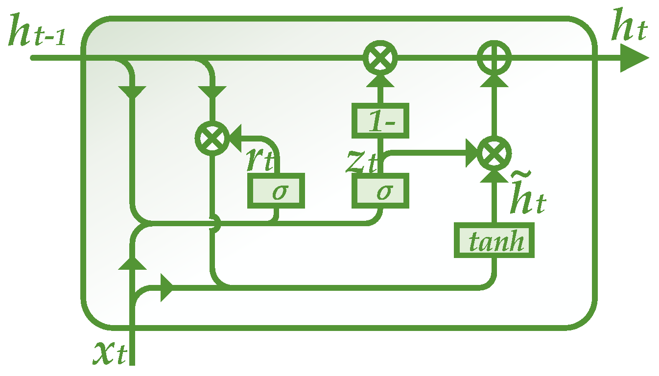
GRU, which is a recently proposed architecture of RNN, is a simplified variant of LSTM [51]. There are mainly two changes in GRU. First, the input and forget gates of LSTM are merged in the model, producing a sole update gate. Second, the two lines in LSTM, that is, the memory and the hidden layer, are also combined together. The integrate structure of GRU is shown in Figure 7. The following equations are designed for calculations in GRU [52]:

$$z_t=\sigma (w_{xz}{x}_t+w_{hz}{h}_{t-1}+b_z),$$

(11)

$$r_t=\sigma (w_{xr}{x}_t+w_{hr}{h}_{t-1}+b_r),$$

(12)

$${\tilde{h}}_t=\tanh (w_{xh}{x}_t+w_{hh}{r}_t{h}_{t-1}+b_h),$$

(13)

$$h_t=(1-z_t)\cdot h_{t-1}+z_t\cdot {\tilde{h}}_t,$$

(14)

where x_t and h_t−1 are the current input and the previous output of GRU, respectively; w_xz, w_hz, w_xr, w_hr, w_xh and w_hh are weights in GRU; b_z, b_r and b_h are biases; z_t, r_t and are outputs during intermediate procedures; and h_t is the final output of the GRU block.

2.4.4. Proposed RNN Structure

In this study, two kinds of RNNs are utilized, that is, the LSTM and the GRU networks. Each RNN has four computation layers, including two recurrent units and two fully-connected layers (also named dense layers). As wind speed data are sampled in the interval of 15 min, a time sequence of wind speed with 48 points is chosen as an input sample by trial and error, which contains historical information of 12 h. Therefore, the input size of the proposed RNNs is 48 × 1. Those deep-learning-based models are established through Tensorflow 1.4.0 [53] and Keras 2.0.8 [54] under Python 3.5.4 and they are trained on a standard PC under Windows 10 operating system with Z270-A motherboard, an Intel Core i7-7700K 4.2 GHz CPU, a NVIDIA GTX 1080 GPU and 16.0 GB of RAM. CUDA Toolkit 9.1 is also utilized. The structures and parameters of RNNs are listed in

Table 1. The structure of the proposed LSTM network.

Layer	Hyper-Parameters	Number of Parameters
LSTM 1	Unit number: 64 Input shape: 48 × 1 Activation: soft sign	16,896
LSTM 2	Unit number: 64 Activation: soft sign	33,024
Dense 1	Unit number: 32	2080
Activation 1	Activation: ReLU	None
Dropout	Rate: 0.00/0.25/0.50	None
Dense 2	Unit number: 1	33
Activation 2	Activation: sigmoid	None
Summary	None	52,033

and

Table 2. The structure of the proposed GRU network.

Layer	Hyper-Parameters	Number of Parameters
GRU 1	Unit number: 64 Input shape: 48 × 1 Activation: soft sign	12,672
GRU 2	Unit number: 64 Activation: soft sign	24,768
Dense 1	Unit number: 32	2080
Activation 1	Activation: ReLU	None
Dropout	Rate: 0.00/0.25/0.50	None
Dense 2	Unit number: 1	33
Activation 2	Activation: sigmoid	None
Summary	None	39,533

, where rectified linear unit (ReLU) and sigmoid are two adopted activation functions:

$${\sigma }_{\mathrm{ReLU}}(x)=\max (x,0),$$

(15)

$${\sigma }_{\mathrm{sigmoid}}(x)=\frac{1}{1+e^{-x}},$$

(16)

From the model structures, the total numbers of trainable parameters in the LSTM and GRU networks are 52,033 and 39,553, respectively. As the number of training samples in this study is more than 70 thousand, the over-fitting problem is effectively avoided. Besides, the computation time for training a RNN sub-model is approximately 380 s (6.3 min), which meets the needs of engineering application. If those sub-models are trained parallel, the entire ensemble model is also suitable for online training and forecasting.

2.5. Adaptive Neuro Fuzzy Inference System (ANFIS) Based Ensemble Approach

The common practice for building ensemble models is to calculate an average value from prediction results of different sub-models. Hence, a quite large number of sub-models is essential. However, due to the long training time of deep-learning-based sub-models, the number of those models is actually limited. Based on this situation, an ANFIS is built in this study as the top layer of the entire ensemble model, in order to fully analyze the small number of sub-models. The final prediction result will be decided by the fuzzy inference system (FIS), which is the output of the ANFIS model.

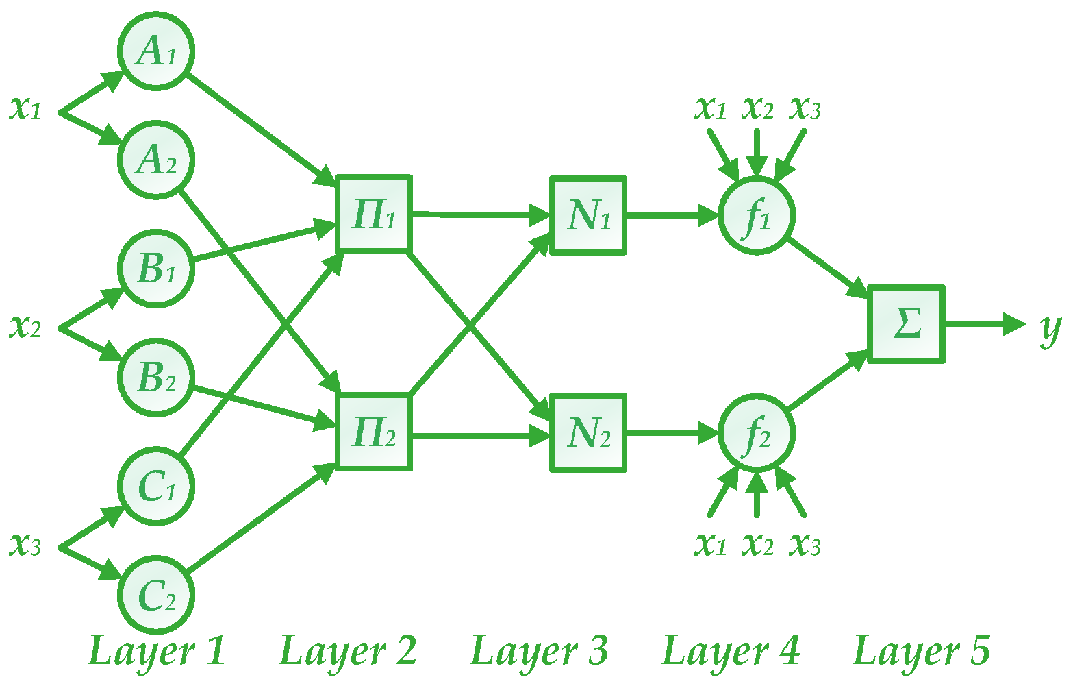
Generally, there are three methods that can establish FIS of an ANFIS model [55]. In consideration of the number of model inputs, an ANFIS with fuzzy-c-means (ANFIS-FCM) is chosen to be utilized. A diagram of ANFIS-FCM is exhibited in Figure 8. The number of fuzzy rules is equal to that of clusters obtained by FCM, as well as that of membership functions (MFs) for each input. In this study, the number of inputs is 6, which is the same number of sub-models. And the number of clusters should be set artificially, which is chosen to be 4 by trial and error.

Based on the architecture of ANFIS-FCM in Figure 8, there are five layers in this model and their computation formulas can be described as follows [56].

• In layer 1, input variables are fuzzified via MFs:

  $$O_{1,i}=\{\begin{array}{ll}{\mu }_{A_i}(x),& i=1,2\\ {\mu }_{B_{i-2}}(x),& i=3,4\\ {\mu }_{C_{i-4}}(x),& i=5,6\end{array},$$

  (17)

  where x and $O_{1,i}$ are the input and the ith output of layer 1, respectively; μ_A, μ_B and μ_C are MFs.
• In layer 2, namely rule layer, the outputs from the previous layer are multiplied together and the firing strengths of rules are calculated:

  $$O_{2,i}=w_i={\mu }_{A_i}(x){\mu }_{B_i}(x){\mu }_{C_i}(x),i=1,2,$$

  (18)
• Layer 3 normalizes the firing strength of each rule as:

  $$O_{3,i}={\overline{w}}_i=w_i/(w_1+w_2),i=1,2,$$

  (19)
• Layer 4 is a defuzzification layer, where adaptive nodes are utilized to calculate the weighted contributions of different rules:

  $$O_{4,i}={\overline{w}}_i{f}_i={\overline{w}}_i(p_i{x}_1+q_i{x}_2+r_i{x}_3+s_i),i=1,2,$$

  (20)

  where p_i, q_i, r_i and s_i are called consequent parameters.
• In layer 5, the final output is obtained by summing contributions of rules:

  $$O_5={\displaystyle {\sum }_i{\overline{w}}_i{f}_i}={\displaystyle {\sum }_i{w}_i{f}_i}/{\displaystyle {\sum }_i{w}_i},i=1,2,$$

  (21)

  where the output is adopted as the point forecasting result of the entire ensemble model.

A hybrid algorithm is commonly used to train ANFIS models. The trainable parameters in ANFIS contain premise parameters in MFs and consequent parameters in layer 4, which are determined via the least square fitting and the gradient descent algorithm, respectively. In this study, the number of inputs is 6, which is the same as that of sub-models. The number of clusters should be set artificially, which is chosen to be 4 by trial and error. The numbers of nodes in layer 2–4 remain the same, which are equal to that of clusters. As a result, the structure of the utilized ANFIS-FCM can be decided, as is shown in

Table 3. The structure of the utilized ANFIS-FCM.

Layer	Number of Nodes	Number of Parameters
Layer 1	24	48
Layer 2	4	None
Layer 3	4	None
Layer 4	4	28
Layer 5	1	None

.

2.6. Probabilistic Forecasting Approach

As wind speed varies randomly and violently, a probabilistic forecasting model can provide more effective information of its future state. In order to measure the range of prediction errors, the uncertainties from the modeling and the forecasting procedures are considered.

The modeling uncertainty is obtained by the variance in sub-models. In the proposed WTD-RNN-ANFIS model, there are six prediction results from RNNs and a result from ANFIS:

$${\tilde{y}}_{\mathrm{e}}(t)=A\left({\tilde{y}}_{si}(t)\right),i=1,2,\cdots ,6,$$

(22)

where ${\tilde{y}}_{\mathrm{e}}(t)$ is the ensemble output of the ANFIS, A(·) is the ANFIS computation, ${\tilde{y}}_{\mathit{si}}(t)$ is the output of the ith sub-model and t is the time to be predicted. Therefore, the modeling uncertainty can be described as the variance:

$${\sigma }_m^2(t)=\frac{1}{6}{\displaystyle \sum _{i=1}^6{\left({\tilde{y}}_{si}(t)-{\tilde{y}}_e(t)\right)}^2},$$

(23)

The final prediction value can hardly be equal to the actual value. As a result, the forecasting uncertainty is produced based on the variance of their differences. The uncertainty is estimated at the training phase, where the actual outputs of the training samples are y(1), y(2), …, y(s). The mean and variance of forecasting differences can be easily calculated as follows:

$$e_f=\frac{1}{s}{\displaystyle \sum _{t=1}^s\left({\tilde{y}}_e(t)-y(t)\right)},$$

(24)

$${\sigma }_f^2=\frac{1}{s}{\displaystyle \sum _{t=1}^s{\left({\tilde{y}}_e(t)-y(t)-e_f\right)}^2},$$

(25)

where s is number of training samples; the variance ${\sigma }_f^2$ denotes the forecasting uncertainty, which is a constant obtained during the training stage.

It is assumed that the above two uncertainties are independent. Therefore, the total uncertainty of the proposed model is the sum of those two parts:

$${\sigma }_t^2(t)={\sigma }_m^2(t)+{\sigma }_f^2.$$

(26)

Based on the uncertainty, the bounds of the prediction interval for confidence level 100·(1−α)% are obtained under the following equations:

$$l_{\alpha }(t)={\tilde{y}}_e(t)-z_{\alpha /2}\cdot \sqrt{{\sigma }_t^2(t)},$$

(27)

$$u_{\alpha }(t)={\tilde{y}}_e(t)+z_{\alpha /2}\cdot \sqrt{{\sigma }_t^2(t)},$$

(28)

where l_α(t) and u_α(t) are the lower and upper bounds of the confidence interval, respectively; z_α/2 is the critical value of a Gaussian distribution.

3. Forecasting Results

In this study, the proposed WTD-RNN-ANFIS model is established to predict wind speed for different steps ahead of time. Other models, including SVM and three-layer ANN, are utilized and compared with the proposed model. Both the point and probabilistic forecasting results are presented based on several performance criteria.

3.1. Performance Criteria

3.1.1. Criteria for Point Forecasting

Root mean square error (RMSE), mean absolute error (MAE) and normalized mean absolute percentage error (NMAPE) are adopted performance criteria for point forecasting in this study. Their calculation equations are as follows:

$$\mathrm{RMSE}=\sqrt{\frac{1}{n}{\displaystyle \sum _{t=1}^n{\left({\tilde{y}}_e(t)-y(t)\right)}^2}},$$

(29)

$$\mathrm{MAE}=\frac{1}{n}{\displaystyle \sum _{t=1}^n\left|{\tilde{y}}_e(t)-y(t)\right|},$$

(30)

$$\mathrm{NMAPE}=\frac{1}{n}{\displaystyle \sum _{t=1}^n\frac{\left|{\tilde{y}}_e(t)-y(t)\right|}{\underset{t\in [1,n]}{\max }y(t)}}\times 100\%,$$

(31)

where n is the number of testing samples. A better prediction performance is achieved when RMSE, MAE and NMAPE are smaller.

3.1.2. Criteria for Probabilistic Forecasting

In this study, average coverage error (ACE) and interval sharpness (IS) are two criteria for evaluating the performance of probabilistic forecasting. ACE is an indicator to appraise the reliability of prediction interval, which has the following equation:

$${\mathrm{ACE}}_{\alpha }=\frac{1}{n}{\displaystyle \sum _{t=1}^n{c}_t\times 100\%-100\cdot (1-\alpha )}\%,$$

(32)

where c_t is the indicative function of coverage and its calculation equation is as:

$$c_t=\{\begin{array}{ll}1,& y(t)\in [l_{\alpha }(t),u_{\alpha }(t)]\\ 0,& y(t)\notin [l_{\alpha }(t),u_{\alpha }(t)]\end{array}.$$

(33)

From the equation of ACE, a value close to zero denotes the high reliability of prediction interval.

As an infinitely wide prediction interval is meaningless, IS is another indicator contrary to the coverage rate of interval, which measures the accuracy of probabilistic forecasting. It can be calculated under the following equation:

$${\mathrm{IS}}_{\alpha }=\frac{1}{n}{\displaystyle \sum _{t=1}^n\{\begin{array}{ll}-2\alpha \left[u_{\alpha }(t)-l_{\alpha }(t)\right]-4\left[l_{\alpha }(t)-y(t)\right],& y(t)<l_{\alpha }(t)\\ -2\alpha \left[u_{\alpha }(t)-l_{\alpha }(t)\right],& y(t)\in [l_{\alpha }(t),u_{\alpha }(t)]\\ -2\alpha \left[u_{\alpha }(t)-l_{\alpha }(t)\right]-4\left[y(t)-u_{\alpha }(t)\right],& y(t)>u_{\alpha }(t)\end{array}}$$

(34)

It can be found that IS_α is always equal to a negative value. A great prediction interval obtains high reliability with a narrow width, which has a small absolute value of IS.

3.2. Denoising Results

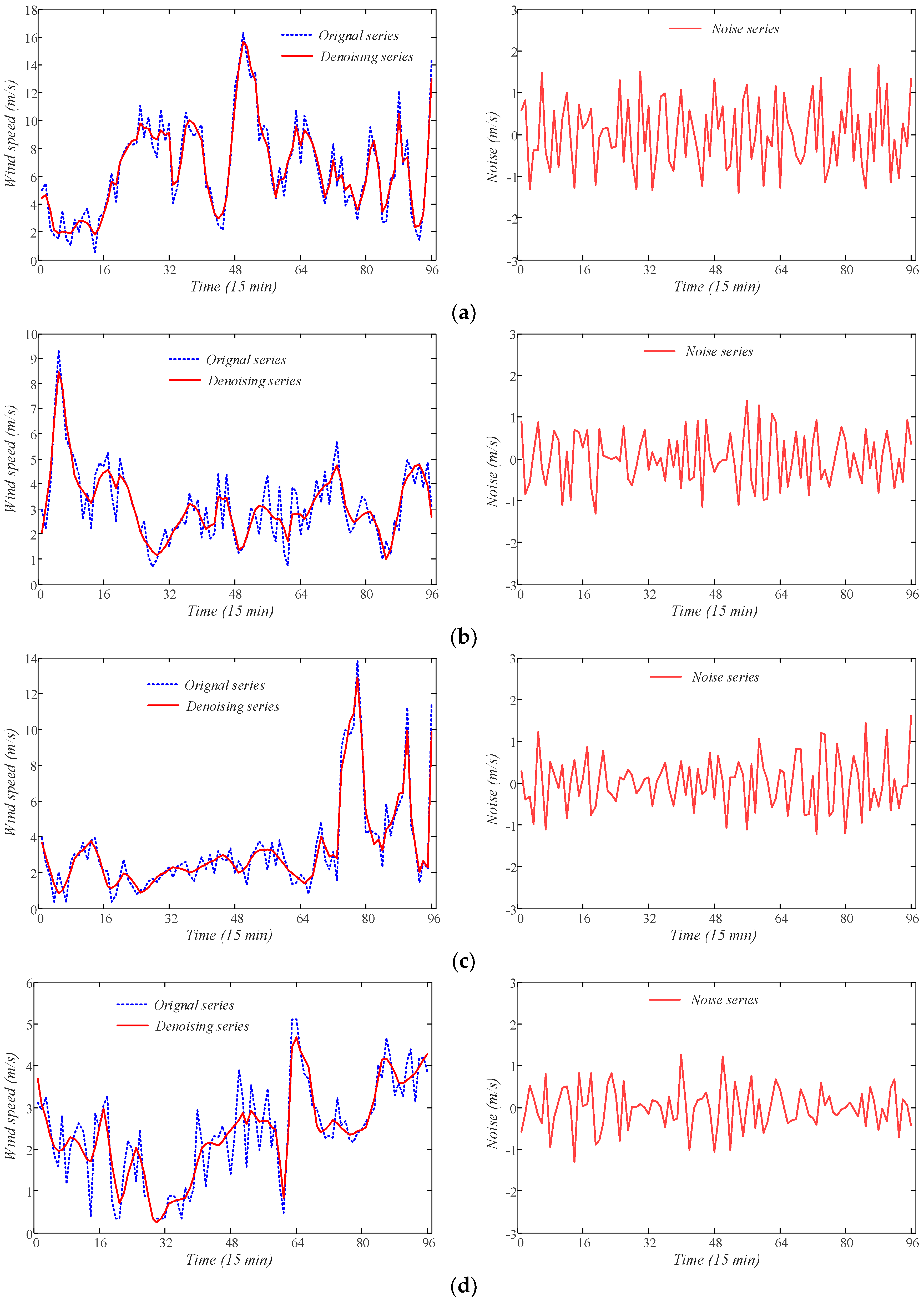
The best parameters of WTD are tried and decided when the highest forecasting accuracy is acquired. In this study, the wavelet basis function, the number of decomposition levels are chosen to be sym4 and 2, respectively. The threshold computation and denoising approaches are selected to be the heuristic algorithm and the soft thresholding method, respectively. Those decomposed series of wind speed are used to construct training and testing samples. In order to display the denoising results, the denoising series in training samples of four days, that is, 1 March, 1 June, 1 September and 1 December in 2016, are presented as examples in Figure 9.

3.3. Point Forecasting Results

In this study, the proposed WTD-RNN-ANFIS model is validated on forecasting wind speed under multi-step-ahead situations, that is, 1-step-ahead (15 min), 2-step-ahead (30 min) and 3-step-ahead (45 min). It is compared with three-layer ANN, SVM, RNN, WTD-ANN, WTD-SVM and WTD-RNN. Specially, the performance criteria in WTD-RNN are the averaged values of the six sub-models in the proposed WTD-RNN-ANFIS, in order to validate the ensemble method that is based on ANFIS. Besides, as mentioned before in Section 2, the wind speed data at 22 March, 23 June, 22 September and 23 December in 2017 are chosen as four testing cases of different seasons.

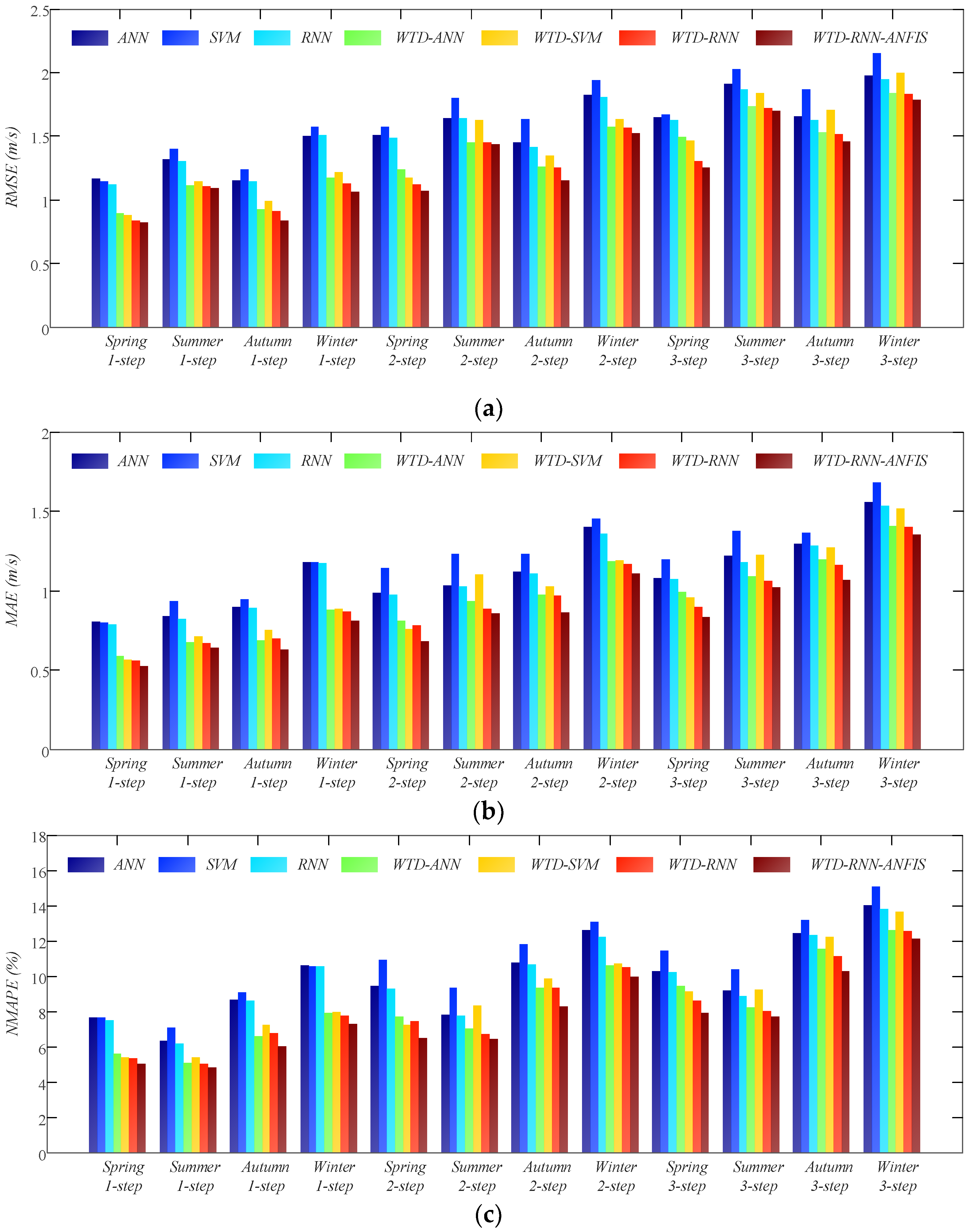
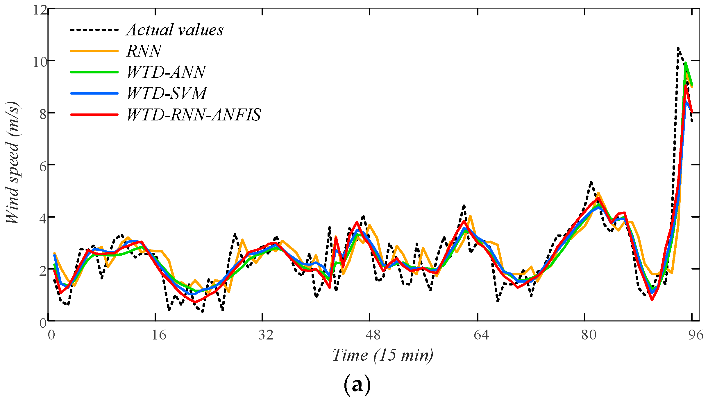
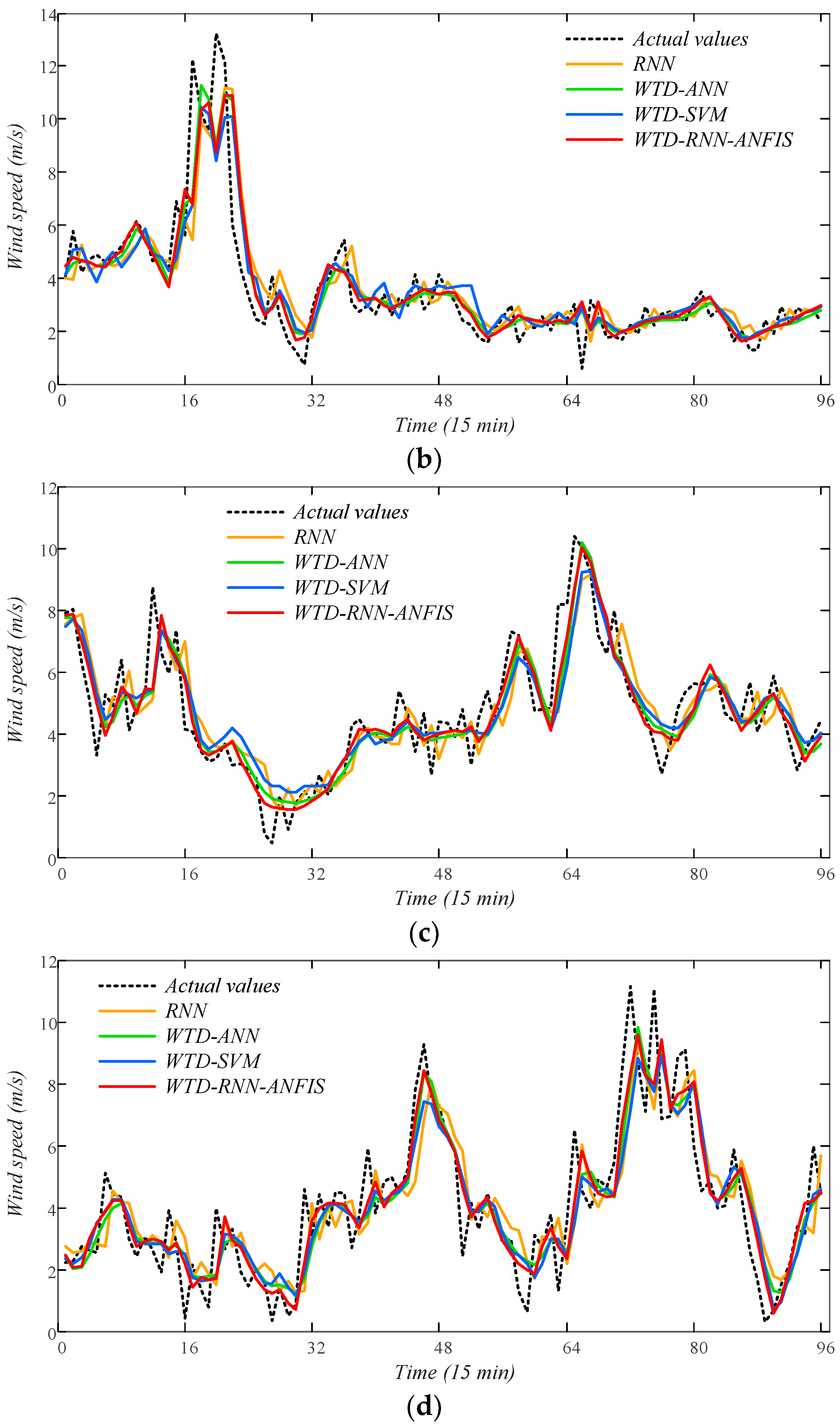
The point forecasting results are presented in

Table 4. The performance criteria of different models for point wind speed forecasting.

Season	Model	1-Step-Ahead			2-Step-Ahead			3-Step-Ahead
		RMSE	MAE	NMAPE	RMSE	MAE	NMAPE	RMSE	MAE	NMAPE
Spring	ANN	1.1676	0.8034	7.6767	1.5123	0.9878	9.4385	1.6500	1.0770	10.2908
	SVM	1.1461	0.7999	7.6433	1.5747	1.1415	10.9071	1.6708	1.1970	11.4368
	RNN	1.1253	0.7860	7.5103	1.4866	0.9709	9.2768	1.6256	1.0718	10.2412
	WTD-ANN	0.8958	0.5871	5.6100	1.2388	0.8087	7.7271	1.4950	0.9895	9.4544
	WTD-SVM	0.8824	0.5650	5.3989	1.1766	0.7553	7.2164	1.4644	0.9541	9.1163
	WTD-RNN	0.8387	0.5608	5.3582	1.1213	0.7792	7.4449	1.3069	0.9003	8.6018
	WTD-RNN-ANFIS	0.8226	0.5261	5.0270	1.0697	0.6823	6.5195	1.2524	0.8316	7.9453
Summer	ANN	1.3205	0.8373	6.3250	1.6402	1.0331	7.8044	1.9126	1.2185	9.2043
	SVM	1.4019	0.9338	7.0542	1.8009	1.2332	9.3159	2.0291	1.3786	10.4139
	RNN	1.3059	0.8206	6.1986	1.6444	1.0264	7.7535	1.8712	1.1770	8.8909
	WTD-ANN	1.1123	0.6739	5.0905	1.4491	0.9314	7.0362	1.7341	1.0919	8.2483
	WTD-SVM	1.1424	0.7134	5.3887	1.6273	1.1049	8.3464	1.8413	1.2233	9.2410
	WTD-RNN	1.1109	0.6679	5.0453	1.4540	0.8883	6.7102	1.7202	1.0640	8.0373
	WTD-RNN-ANFIS	1.0929	0.6410	4.8420	1.4330	0.8554	6.4617	1.7021	1.0185	7.6939
Autumn	ANN	1.1547	0.8981	8.6419	1.4514	1.1184	10.7618	1.6540	1.2927	12.4394
	SVM	1.2365	0.9430	9.0740	1.6358	1.2294	11.8301	1.8663	1.3675	13.1595
	RNN	1.1436	0.8919	8.5824	1.4171	1.1079	10.6614	1.6299	1.2848	12.3633
	WTD-ANN	0.9238	0.6854	6.5955	1.2646	0.9723	9.3561	1.5324	1.1980	11.5280
	WTD-SVM	0.9903	0.7496	7.2130	1.3523	1.0248	9.8611	1.7073	1.2700	12.2206
	WTD-RNN	0.9100	0.7006	6.7421	1.2563	0.9694	9.3281	1.5174	1.1585	11.1482
	WTD-RNN-ANFIS	0.8371	0.6270	6.0333	1.1504	0.8609	8.2839	1.4619	1.0671	10.2689
Winter	ANN	1.4992	1.1780	10.5903	1.8225	1.4006	12.5916	1.9744	1.5596	14.0211
	SVM	1.5738	1.1762	10.5745	1.9390	1.4541	13.0726	2.1495	1.6796	15.0998
	RNN	1.5076	1.1710	10.5278	1.8090	1.3623	12.2480	1.9499	1.5373	13.8208
	WTD-ANN	1.1708	0.8830	7.9384	1.5748	1.1821	10.6272	1.8417	1.4049	12.6303
	WTD-SVM	1.2165	0.8884	7.9867	1.6361	1.1929	10.7250	1.9997	1.5163	13.6325
	WTD-RNN	1.1263	0.8663	7.7883	1.5652	1.1676	10.4973	1.8326	1.3983	12.5713
	WTD-RNN-ANFIS	1.0641	0.8123	7.3025	1.5236	1.1108	9.9867	1.7849	1.3511	12.1470
Overall	ANN	1.2930	0.9292	7.0191	1.6052	1.1324	8.5539	1.8038	1.2869	9.7216
	SVM	1.3495	0.9632	7.2763	1.7435	1.2646	9.5525	1.9373	1.4057	10.6184
	RNN	1.2799	0.9174	6.9298	1.6041	1.1195	8.4568	1.7750	1.2677	9.5764
	WTD-ANN	1.0272	0.7074	5.3434	1.3737	0.9662	7.2991	1.6390	1.1624	8.7811
	WTD-SVM	1.0659	0.7291	5.5075	1.4610	1.0195	7.7011	1.7641	1.2409	9.3740
	WTD-RNN	1.0045	0.6989	5.2795	1.3649	0.9585	7.2405	1.6097	1.1389	8.6032
	WTD-RNN-ANFIS	0.9678	0.6516	4.9221	1.3079	0.8774	6.6276	1.5643	1.0671	8.0608

¹ The numbers in bold are the best criteria of each studied case.

, where the best criteria of each case are emphasized in bold and the comparisons of those criteria are shown in Figure 10. From the results, it can be found that WTD is a great pre-processing method in wind speed forecasting, as it reduces the uncertainties of wind speed variation. The comparisons indicate that SVM performs worse than ANN and RNN. Besides, SVM costs rather long computation time when trained on a large number of training samples, which is not suitable for online training of short-term forecasting. It is noted that RNN usually achieves better performance than ANN whether or not WTD is utilized. The proposed WTD-RNN-ANFIS obtains the best forecasting results in all four cases. Therefore, it is a perfect ensemble model for short-term wind speed forecasting rather than just calculating an averaged output from different sub-models. Moreover, the prediction curves of 1-step-ahead point forecasting using several representative models are presented as examples in Figure 11. The curve of the proposed WTD-RNN-ANFIS fits the actual value best, which denotes the superb point forecasting performance of the model.

3.4. Probabilistic Forecasting Results

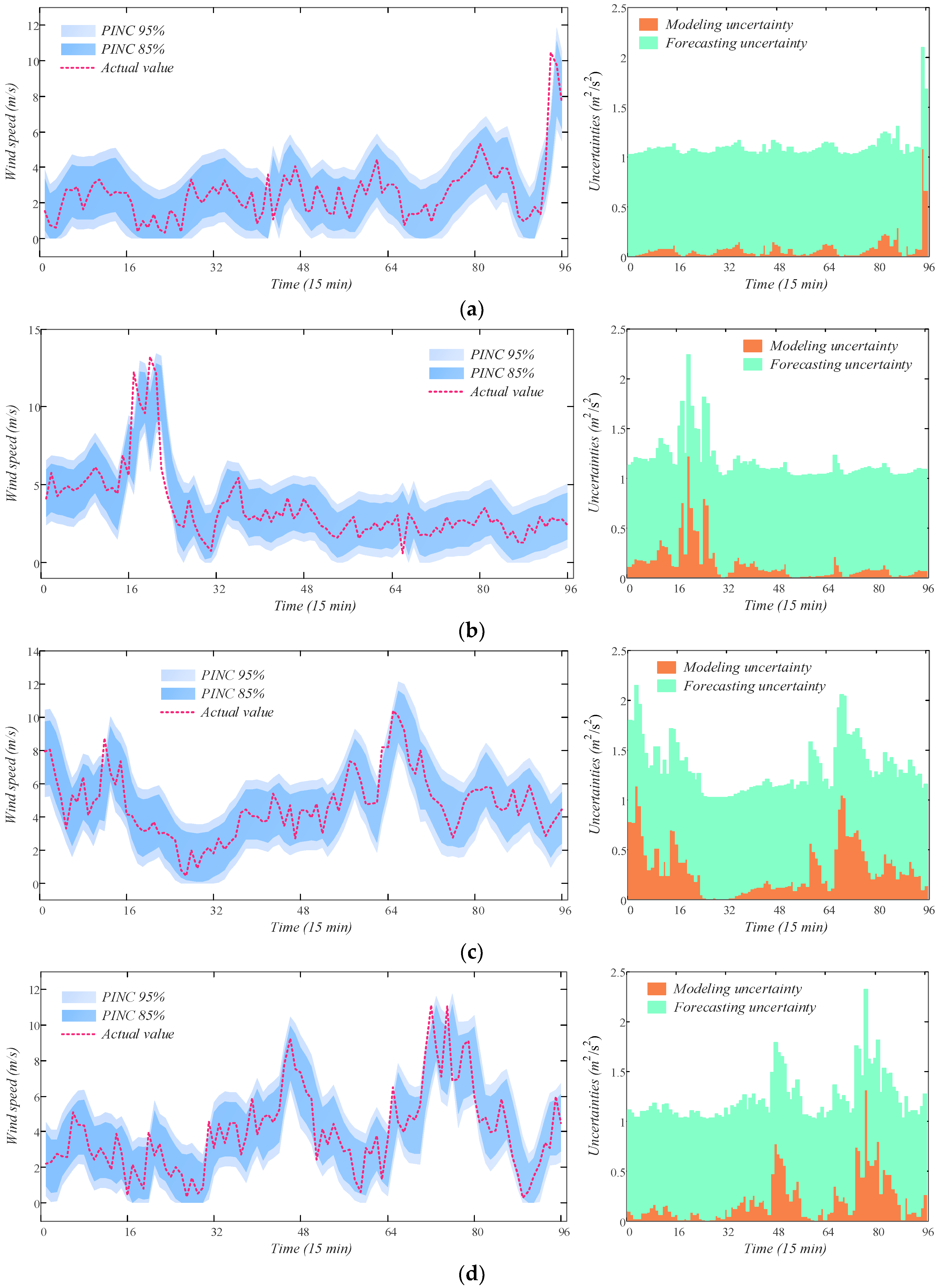
In order to validate the feasibility of the proposed WTD-RNN-ANFIS model for probabilistic wind speed forecasting, we establish it to calculate the prediction intervals of wind speed under 1~3 steps ahead timescales. Different prediction interval nominal confidences (PINCs) are verified in this study, including 85%, 90% and 95%. The comparison results based on criteria ACE and IS are presented in

Table 5. The criterion ACE (%) of probabilistic wind speed forecasting using WTD-RNN-ANFIS.

Time Scale	PINC (%)	Spring	Summer	Autumn	Winter	Overall
1-step-ahead	85	10.83	7.71	11.88	2.50	8.23
	90	6.88	3.75	7.92	0.63	4.79
	95	1.88	−0.21	2.92	−1.25	0.83
2-step-ahead	85	12.92	4.58	8.75	−0.63	6.41
	90	6.88	1.67	−4.58	−3.54	0.10
	95	2.92	−3.33	1.88	−2.29	−0.21
3-step-ahead	85	11.88	1.46	7.71	1.46	5.63
	90	7.92	−1.46	5.83	−0.42	2.97
	95	2.92	−0.21	0.83	−0.21	0.83

and

Table 6. The criterion IS of probabilistic wind speed forecasting using WTD-RNN-ANFIS.

Time Scale	PINC (%)	Spring	Summer	Autumn	Winter	Overall
1-step-ahead	85	−1.10	−1.41	−1.10	−1.25	−1.21
	90	−0.86	−1.12	−0.84	−0.91	−0.93
	95	−0.54	−0.75	−0.50	−0.52	−0.58
2-step-ahead	85	−1.48	−1.52	−1.47	−1.87	−1.60
	90	−1.12	−1.25	−1.11	−1.38	−1.21
	95	−0.72	−0.70	−0.63	−0.79	−0.71
3-step-ahead	85	−1.73	−1.76	−1.83	−2.09	−1.86
	90	−1.32	−1.36	−1.33	−1.54	−1.38
	95	−0.81	−0.78	−0.76	−0.88	−0.82

. From the results, the criteria ACE and IS maintain within certain ranges in all verified time scales, which indicates that the proposed WTD-RNN-ANFIS model achieves a rather high reliability in ultra-short probabilistic forecasting. Moreover, prediction intervals of 1-step-ahead forecasting obtained by the proposed model under four cases are shown as examples in Figure 12. It can be discovered that the intervals cover the actual series of wind speed perfectly.

4. Comparisons and Discussion

In this section, in order to fully verify the superiority of the proposed model, we further compare different probabilistic forecasting models for 1-step-ahead wind speed forecasting. The tested PINCs are also chosen to be 85%, 90% and 95%. In addition to the proposed WTD-RNN-ANFIS, we establish another 4 models that have been introduced in the literatures. In Reference [57], He et al. proposed a probability density forecasting method based on Copula theory and support vector quantile regression (SVQR). Similarly, He et al. [58] proposed another probability density forecasting method based on quantile regression neural network (QRNN) and kernel density estimation. Those two models both utilize quantile regression (QR) to calculate prediction intervals and will be compared with the proposed model in this study. In Reference [59], a probabilistic wind speed forecasting model is introduced by Hu et al., which consists of empirical wavelet transform (EWT) and GPR. GPR is a non-parametric estimation method that defines mean and variance functions, where the variance can be directly used for probabilistic forecasting. Moreover, in order to validate the proposed probabilistic forecasting approach that is based on variances of sub-models, we compute modeling and forecasting uncertainties using another ensemble model [60] for comparison. It is introduced by Lee et al. that calculates an averaged result from random forest, gradient boosting machine (GBM), ridge regression, auto-regressive (AR) model and AR with exogenous (ARX). Their comparisons based on criteria ACE and IS are shown in

Table 7. Comparisons of the criterion ACE (%) for probabilistic wind speed forecasting.

Model	PINC (%)	Spring	Summer	Autumn	Winter	Overall
He et al. [57]	85	−14.18	−11.04	−14.17	−13.13	−13.13
	90	−11.88	−4.58	−4.58	−12.92	−8.49
	95	−3.33	−5.42	−4.38	−8.54	−5.42
He et al. [58]	85	−13.13	−11.04	−14.17	−12.08	−12.60
	90	−12.92	−6.67	−4.58	−12.92	−9.27
	95	−5.42	−5.42	−3.33	−10.63	−6.20
Hu et al. [59]	85	11.88	13.96	11.88	10.83	12.14
	90	8.96	8.96	7.92	10.00	8.96
	95	3.96	3.96	2.92	5.00	3.96
Lee et al. [60]	85	12.92	8.75	8.75	4.58	8.75
	90	8.96	4.79	5.83	2.71	5.57
	95	3.96	1.88	3.96	−2.29	−1.88
WTD-RNN-ANFIS	85	10.83	7.71	11.88	2.50	8.23
	90	6.88	3.75	7.92	0.63	4.79
	95	1.88	−0.21	2.92	−1.25	0.83

The numbers in bold are the best criteria of each studied case.

and

Table 8. Comparisons of the criterion IS for probabilistic wind speed forecasting.

Model	PINC (%)	Spring	Summer	Autumn	Winter	Overall
He et al. [57]	85	−1.55	−1.55	−1.43	−2.39	−1.73
	90	−1.22	−1.20	−1.07	−1.88	−1.34
	95	−0.79	−0.72	−0.63	−1.18	−0.83
He et al. [58]	85	−1.57	−1.55	−1.49	−2.41	−1.75
	90	−1.14	−1.15	−1.09	−1.77	−1.29
	95	−0.78	−0.69	−0.64	−1.19	−0.82
Hu et al. [59]	85	−1.50	−1.89	−1.94	−2.01	−1.84
	90	−1.14	−1.76	−1.45	−1.48	−1.46
	95	−0.72	−0.99	−0.83	−0.84	−0.85
Lee et al. [60]	85	−1.44	−1.73	−1.47	−1.76	−1.60
	90	−1.10	−1.34	−1.10	−1.26	−1.20
	95	−0.69	−0.87	−0.64	−0.68	−0.72
WTD-RNN-ANFIS	85	−1.10	−1.41	−1.10	−1.25	−1.21
	90	−0.86	−1.12	−0.84	−0.91	−0.93
	95	−0.54	−0.75	−0.50	−0.52	−0.58

The numbers in bold are the best criteria of each studied case.

.

From the comparison results, the two QR models obtains the worst criterion of ACE and GPR acquires the worst criterion of IS. According to the comparison between QR and GPR, QR merely achieves better IS than GPR whereas it can hardly cover the actual wind speed series. The reason may be that QR extremely concentrates on achieving the minimum quantile loss function so that it ignores the coverage rate. It is to say otherwise that machine-learning-based QR model reveals no significant merits in probabilistic forecasting. As a result, the QR models in Reference [57,58] adopt kernel destiny estimation method to ameliorate this situation and improve forecasting performance. Besides, those two kinds of models, QR and GPR, calculate prediction intervals directly based on the distribution of historical time series whereas the unavoidable forecasting errors in models are not included. On the contrary, we involve forecasting errors as forecasting uncertainties in our proposed probabilistic forecasting approach and test two ensemble models, that is, the model proposed by Lee et al. [60] and WTD-RNN-ANFIS. The two models achieve better ACE and slightly improve the IS. Hence, the proposed probabilistic forecasting approach increases the prediction reliability of models without enlarging their widths of prediction intervals. Moreover, WTD-RNN-ANFIS performs better than the ensemble model in Reference [60], probably due to the denoising procedure of WTD and the strong learning ability of RNN.

As the forecasting accuracy of wind speed further increases owing to the proposed WTD-RNN-ANFIS model, especially ultra-short-term forecasting, it can help the operators of wind power integrated system to better guide the real-time scheduling and dispatching of electrical power system. In this study, we mainly introduce state-of-the-art technologies of ensemble learning and deep learning into the field of renewable energy forecasting, in order to improve the operation reliability and security of power system. If the acquisition and storage technology for real-time data can be improved, as well as the calculation capability in power system, its operators will benefit much more from the contributions of the study. Moreover, we provide a feasible probabilistic forecasting approach based on deep learning without adding too much calculation burden. However, it still remains limitations that merely one kind of sub-model is utilized in ensemble and the prediction accuracy is not greatly enhanced due to the rapid fluctuation of wind speed. Therefore, it is of great application value to research and verify more deep-learning-based models for renewable energy forecasting and it will be involved in our future work.

5. Conclusions

An ensemble WTD-RNN-ANFIS model is proposed in this study for probabilistic wind speed forecasting. The model is based on wavelet decomposition, deep learning and ensemble learning technologies. It is aimed at less than one-hour-ahead ultra-short-term forecasting of wind speed, which utilizes historical wind speed data as inputs. We compare the proposed model with other commonly-used machine learning models to predict wind speed based on four cases of different seasons and the prediction results are in both point and interval forms.

From the comparisons, WTD evidently reduces the volatilities and uncertainties in wind speed series, so that forecasting models can better capture the variation trend of wind speed and improve their prediction accuracies. A RNN model, which are based on deep learning technology, is able to learn the correlations among data points in an entire time series. It is proved to achieve better results in wind speed forecasting than shallow ANN in this study. Besides, ANFIS successfully increases prediction accuracy of the ensemble model using only a small number of sub-models. It performs better than the ensemble model that merely calculates an averaged output value from sub-models.

Specifically, based on the overall testing datasets, the criteria RMSE, MAE and NMAPE of the proposed model in 15-min-ahead forecasting reach 0.9678 m/s, 0.6516 m/s and 4.9221%, respectively. Those criteria in 30-min-ahead and 45-min-ahead forecasting are 1.3079 m/s and 1.5643 m/s, 0.8774 m/s and 1.0671 m/s, 6.6276% and 8.0608%, respectively. The above prediction results indicate the superiority of the proposed ensemble model in ultra-short point wind speed forecasting. The high forecasting accuracy of the proposed model can meet the needs of practical engineering projects, which can benefit the secure operations of wind power integrated system. Moreover, the best ACE and IS of the proposed model tested on the overall datasets are −0.21% and −0.58, respectively. Comparing to traditional QR models, it achieves more reliable prediction intervals, demonstrating its excellent performance in ultra-short probabilistic wind speed forecasting.

As wind speed fluctuates rapidly and arbitrarily, the improvement in performance of prediction models is limited. Therefore, it is desired that in the future advanced signal decomposition and denoising technologies can be adopted and merged into hybrid wind speed forecasting methods. Besides, the ensemble model proposed in this study merely utilizes RNNs as sub-models. It remains to be studied further that other state-of-the-art deep-learning-based models are combined for ensemble learning.

References

- Wang, J.Z.; Qin, S.S.; Jin, S.Q.; Wu, J. Estimation methods review and analysis of offshore extreme wind speeds and wind energy resources. Renew. Sustain. Energy Rev. 2015, 42, 26–42. [Google Scholar] [CrossRef]
- Sahu, B.K. Wind energy developments and policies in China: A short review. Renew. Sustain. Energy Rev. 2018, 81, 1393–1405. [Google Scholar] [CrossRef]
- Ogliari, E.; Dolara, A.; Manzolini, G.; Leva, S. Physical and hybrid methods comparison for the day ahead PV output power forecast. Renew. Energy 2017, 113, 11–21. [Google Scholar] [CrossRef] [Green Version]
- Jung, J.; Broadwater, R.P. Current status and future advances for wind speed and power forecasting. Renew. Sustain. Energy Rev. 2014, 31, 762–777. [Google Scholar] [CrossRef]
- Wang, J.Z.; Song, Y.L.; Liu, F.; Hou, R. Analysis and application of forecasting models in wind power integration: A review of multi–step–ahead wind speed forecasting models. Renew. Sustain. Energy Rev. 2016, 60, 960–981. [Google Scholar] [CrossRef]
- Okumus, I.; Dinler, A. Current status of wind energy forecasting and a hybrid method for hourly predictions. Energy Convers. Manag. 2016, 123, 362–371. [Google Scholar] [CrossRef]
- You, Q.L.; Fraedrich, K.; Min, J.Z.; Kang, S.C.; Zhu, X.H.; Pepin, N.; Zhang, L. Observed surface wind speed in the Tibetan Plateau since 1980 and its physical causes. Int. J. Climatol. 2014, 34, 1873–1882. [Google Scholar] [CrossRef] [Green Version]
- Chen, L.; Li, D.; Pryor, S.C. Wind speed trends over China: Quantifying the magnitude and assessing causality. Int. J. Climatol. 2013, 33, 2579–2590. [Google Scholar] [CrossRef]
- Erdem, E.; Shi, J. ARMA based approaches for forecasting the tuple of wind speed and direction. Appl. Energy 2011, 88, 1405–1414. [Google Scholar] [CrossRef]
- Kavasseri, R.G.; Seetharaman, K. Day-ahead wind speed forecasting using f-ARIMA models. Renew. Energy 2009, 34, 1388–1393. [Google Scholar] [CrossRef]
- Shukur, O.B.; Lee, M.H. Daily wind speed forecasting through hybrid KF-ANN model based on ARIMA. Renew. Energy 2015, 76, 637–647. [Google Scholar] [CrossRef]
- Zhao, E.D.; Zhao, J.; Liu, L.W.; Su, Z.Y.; An, N. Hybrid Wind Speed Prediction Based on a Self-Adaptive ARIMAX Model with an Exogenous WRF Simulation. Energies 2016, 9, 7. [Google Scholar] [CrossRef]
- Leva, S.; Dolara, A.; Grimaccia, F.; Mussetta, M.; Ogliari, E. Analysis and validation of 24 hours ahead neural network forecasting of photovoltaic output power. Math. Comput. Simul. 2017, 131, 88–100. [Google Scholar] [CrossRef] [Green Version]
- Zjavka, L. Wind speed forecast correction models using polynomial neural networks. Renew. Energy 2015, 83, 998–1006. [Google Scholar] [CrossRef]
- Chang, G.W.; Lu, H.J.; Chang, Y.R.; Lee, Y.D. An improved neural network-based approach for short-term wind speed and power forecast. Renew. Energy 2017, 105, 301–311. [Google Scholar] [CrossRef]
- Ogliari, E.; Niccolai, A.; Leva, S.; Zich, R. Computational intelligence techniques applied to the day ahead pv output power forecast: phann, sno and mixed. Energies 2018, 11, 1487. [Google Scholar] [CrossRef]
- Yang, L.; He, M.; Zhang, J.S.; Vittal, V. Support-vector-machine-enhanced markov model for short-term wind power forecast. IEEE Trans. Sustain. Energy 2015, 6, 791–799. [Google Scholar] [CrossRef]
- De Giorgi, M.G.; Campilongo, S.; Ficarella, A.; Congedo, P.M. Comparison between wind power prediction models based on wavelet decomposition with least-squares support vector machine (LS-SVM) and artificial neural network (ANN). Energies 2014, 7, 5251–5272. [Google Scholar] [CrossRef]
- Wu, Q.L.; Peng, C.Y. Wind power generation forecasting using least squares support vector machine combined with ensemble empirical mode decomposition, principal component analysis and a bat algorithm. Energies 2016, 9, 261. [Google Scholar] [CrossRef]
- Zhao, Y.N.; Ye, L.; Li, Z.; Song, X.R.; Lang, Y.S.; Su, J. A novel bidirectional mechanism based on time series model for wind power forecasting. Appl. Energy 2016, 177, 793–803. [Google Scholar] [CrossRef]
- Wan, C.; Xu, Z.; Pinson, P.; Dong, Z.Y.; Wong, K.P. Probabilistic forecasting of wind power generation using extreme learning machine. IEEE Trans. Power Syst. 2014, 29, 1033–1044. [Google Scholar] [CrossRef]
- Huang, N.T.; Yuan, C.; Cai, G.W.; Xing, E.K. Hybrid short term wind speed forecasting using variational mode decomposition and a weighted regularized extreme learning machine. Energies 2016, 9, 989. [Google Scholar] [CrossRef]
- Liu, H.; Tian, H.Q.; Li, Y.F. Comparison of new hybrid FEEMD-MLP, FEEMD-ANFIS, Wavelet Packet-MLP and Wavelet Packet-ANFIS for wind speed predictions. Energy Convers. Manag. 2015, 89, 1–11. [Google Scholar] [CrossRef]
- Wang, H.Z.; Wang, G.B.; Li, G.Q.; Peng, J.C.; Liu, Y.T. Deep belief network based deterministic and probabilistic wind speed forecasting approach. Appl. Energy 2016, 182, 80–93. [Google Scholar] [CrossRef]
- Khodayar, M.; Kaynak, O.; Khodayar, M.E. Rough deep neural architecture for short-term wind speed forecasting. IEEE Trans. Ind. Inform. 2017, 13, 2770–2779. [Google Scholar] [CrossRef]
- Qureshi, A.S.; Khan, A.; Zameer, A.; Usman, A. Wind power prediction using deep neural network based meta regression and transfer learning. Appl. Soft Comput. 2017, 58, 742–755. [Google Scholar] [CrossRef]
- Wang, H.-z.; Li, G.-q.; Wang, G-b.; Peng, J-c.; Jiang, H.; Liu, Y-t. Deep learning based ensemble approach for probabilistic wind power forecasting. Appl. Energy 2017, 188, 56–70. [Google Scholar] [CrossRef]
- Liu, H.; Mi, X.W.; Li, Y.F. Wind speed forecasting method based on deep learning strategy using empirical wavelet transform, long short term memory neural network and Elman neural network. Energy Convers. Manag. 2018, 156, 498–514. [Google Scholar] [CrossRef]
- Liu, H.; Mi, X.W.; Li, Y.F. Smart multi-step deep learning model for wind speed forecasting based on variational mode decomposition, singular spectrum analysis, LSTM network and ELM. Energy Convers. Manag. 2018, 159, 54–64. [Google Scholar] [CrossRef]
- Baek, M.K.; Lee, D. Spatial and temporal day-ahead total daily solar irradiation forecasting: ensemble forecasting based on the empirical biasing. Energies 2018, 11, 70. [Google Scholar] [CrossRef]
- Ren, Y.; Suganthan, P.N.; Srikanth, N. Ensemble methods for wind and solar power forecasting-A state-of-the-art review. Renew. Sustain. Energy Rev. 2015, 50, 82–91. [Google Scholar] [CrossRef]
- Tascikaraoglu, A.; Uzunoglu, M. A review of combined approaches for prediction of short-term wind speed and power. Renew. Sustain. Energy Rev. 2014, 34, 243–254. [Google Scholar] [CrossRef]
- Lee, D.; Baldick, R. Short-Term Wind power ensemble prediction based on gaussian processes and neural networks. IEEE Trans. Smart Grid 2014, 5, 501–510. [Google Scholar] [CrossRef]
- Peng, T.; Zhou, J.Z.; Zhang, C.; Zheng, Y. Multi-step ahead wind speed forecasting using a hybrid model based on two-stage decomposition technique and AdaBoost-extreme learning machine. Energy Convers. Manag. 2017, 153, 589–602. [Google Scholar] [CrossRef]
- Wu, W.B.; Peng, M. A data mining approach combining k-means clustering with bagging neural network for short-term wind power forecasting. IEEE Int. Things 2017, 4, 979–986. [Google Scholar] [CrossRef]
- Jager, D.; Andreas, A. NREL National Wind Technology Center (NWTC): M2 Tower; Boulder, Colorado (Data). Available online: https://www.osti.gov/biblio/1052222-nrel-national-wind-technology-center-nwtc-m2-tower-boulder-colorado-data (accessed on 24 July 2018).
- Morshedizadeh, M.; Kordestani, M.; Carriveau, R.; Ting, D.S.K.; Saif, M. Application of imputation techniques and Adaptive Neuro-Fuzzy Inference System to predict wind turbine power production. Energy 2017, 138, 394–404. [Google Scholar] [CrossRef]
- Eynard, J.; Grieu, S.; Polit, M. Wavelet-based multi-resolution analysis and artificial neural networks for forecasting temperature and thermal power consumption. Eng. Appl. Artif. Intell. 2011, 24, 501–516. [Google Scholar] [CrossRef] [Green Version]
- Adamowski, J.; Chan, H.F. A wavelet neural network conjunction model for groundwater level forecasting. J. Hydrol. 2011, 407, 28–40. [Google Scholar] [CrossRef]
- Lee, W.S.; Kassim, A.A. Signal and image approximation using interval wavelet transform. IEEE Trans. Image Process 2007, 16, 46–56. [Google Scholar] [CrossRef] [PubMed]
- Sharma, V.; Yang, D.Z.; Walsh, W.; Reindl, T. Short term solar irradiance forecasting using a mixed wavelet neural network. Renew. Energy 2016, 90, 481–492. [Google Scholar] [CrossRef]
- Chemali, E.; Kollmeyer, P.J.; Preindl, M.; Ahmed, R.; Emadi, A. Long short-term memory networks for accurate state-of-charge estimation of li-ion batteries. IEEE Trans. Ind. Electron. 2018, 65, 6730–6739. [Google Scholar] [CrossRef]
- Guo, D.S.; Zhang, Y.N. Novel Recurrent Neural Network for Time-Varying Problems Solving. IEEE Comput. Intell. Mag. 2012, 7, 61–65. [Google Scholar] [CrossRef]
- Sundermeyer, M.; Ney, H.; Schluter, R. From feedforward to recurrent lstm neural networks for language modeling. IEEE Trans. Audio Speech Lang. Process. 2015, 23, 517–529. [Google Scholar] [CrossRef]
- Moretti, F.; Pizzuti, S.; Panzieri, S.; Annunziato, M. Urban traffic flow forecasting through statistical and neural network bagging ensemble hybrid modeling. Neurocomputing 2015, 167, 3–7. [Google Scholar] [CrossRef]
- Srivastava, N.; Hinton, G.; Krizhevsky, A.; Sutskever, I.; Salakhutdinov, R. Dropout: A simple way to prevent neural networks from overfitting. J. Mach. Learn. Res. 2014, 15, 1929–1958. [Google Scholar]
- Srivastava, S.; Lessmann, S. A comparative study of LSTM neural networks in forecasting day-ahead global horizontal irradiance with satellite data. Sol. Energy 2018, 162, 232–247. [Google Scholar] [CrossRef]
- Hochreiter, S.; Schmidhuber, J. Long short-term memory. Neural. Comput. 1997, 9, 1735–1780. [Google Scholar] [CrossRef] [PubMed]
- Hochreiter, S. The vanishing gradient problem during learning recurrent neural nets and problem solutions. Int. J. Uncertain. Fuzziness Knowl.-Based Syst. 1998, 6, 107–116. [Google Scholar] [CrossRef]
- Graves, A. Supervised Sequence Labelling with Recurrent Neural Networks. Stud. Comput. Intell. 2012, 385, 1–141. [Google Scholar]
- Zhao, R.; Wang, D.Z.; Yan, R.Q.; Mao, K.Z.; Shen, F.; Wang, J.J. Machine health monitoring using local feature-based gated recurrent unit networks. IEEE Trans. Ind. Electron. 2018, 65, 1539–1548. [Google Scholar] [CrossRef]
- Le, T.H.N.; Quach, K.G.; Luu, K.; Duong, C.N.; Savvides, M. Reformulating Level Sets as Deep Recurrent Neural Network Approach to Semantic Segmentation. IEEE Trans. Image Process. 2018, 27, 2393–2407. [Google Scholar] [CrossRef] [PubMed] [Green Version]
- Wongsuphasawat, K.; Smilkov, D.; Wexler, J.; Wilson, J.; Mane, D.; Fritz, D.; Krishnan, D.; Viegas, F.B.; Wattenberg, M. Visualizing dataflow graphs of deep learning models in tensorflow. IEEE Trans. Vis. Comput. Graph. 2018, 24, 1–12. [Google Scholar] [CrossRef] [PubMed]
- Aguiam, D.E.; Silva, A.; Guimarais, L.; Carvalho, P.J.; Conway, G.D.; Goncalves, B.; Meneses, L.; Noterdaeme, J.M.; Santos, J.M.; Tuccillo, A.A.; et al. Estimation of x-mode reflectometry first fringe frequency using neural networks. IEEE Trans. Plasma Sci. 2018, 46, 1323–1330. [Google Scholar] [CrossRef]
- Kisi, O.; Demir, V.; Kim, S. Estimation of long-term monthly temperatures by three different adaptive neuro-fuzzy approaches using geographical inputs. J. Irrig. Drain. Eng. 2017, 143, 401–421. [Google Scholar] [CrossRef]
- Mohammadi, K.; Shamshirband, S.; Tong, C.W.; Alam, K.A.; Petković, D. Potential of adaptive neuro-fuzzy system for prediction of daily global solar radiation by day of the year. Energy Convers. Manag. 2015, 93, 406–413. [Google Scholar] [CrossRef]
- He, Y.; Liu, R.; Li, H.; Wang, S.; Lu, X. Short-term power load probability density forecasting method using kernel-based support vector quantile regression and Copula theory. Appl. Energy 2017, 185, 254–266. [Google Scholar] [CrossRef]
- He, Y.Y.; Li, H.Y. Probability density forecasting of wind power using quantile regression neural network and kernel density estimation. Energy Convers. Manag. 2018, 164, 374–384. [Google Scholar] [CrossRef]
- Hu, J.M.; Wang, J.Z. Short-term wind speed prediction using empirical wavelet transform and Gaussian process regression. Energy 2015, 93, 1456–1466. [Google Scholar] [CrossRef]
- Lee, D.; Park, Y.G.; Park, J.B.; Roh, J.H. Very Short-Term Wind Power Ensemble Forecasting without Numerical Weather Prediction through the Predictor Design. J. Electr. Eng. Technol. 2017, 12, 2177–2186. [Google Scholar]
Figure 1.
The monthly averaged wind speed of datasets in years 2015–2017.
Figure 2.
The entire architecture of the proposed probabilistic forecasting model.
Figure 3.
A three-level decomposition of discrete wavelet transform (DWT) using Mallat algorithm.
Figure 4.
The sequential structure of recurrent neural network (RNN).
Figure 5.
A dropout layer with rate p = 0.25. (a) dropout during the training phase; (b) dropout during the testing phase.
Figure 6.
The structure of a long short-term memory (LSTM) block.
Figure 7.
The structure of a gated recurrent unit (GRU) block.
Figure 8.
An example model of adaptive neural fuzzy inference system-fuzzy c-means (ANFIS-FCM) with 3 inputs and 2 clusters.
Figure 9.
The denoising results of wind speed series using WTD. (a) 1 March 2016; (b) 1 June 2016; (c) 1 September 2016; (d) 1 December 2016.
Figure 10.
The comparisons of performance criteria for point wind speed forecasting. (a) RMSE; (b) MAE; (c) NMAPE.
Figure 11.
The prediction curves of 1-step-ahead point wind speed forecasting. (a) Spring; (b) summer; (c) autumn; (d) winter.
Figure 12.
The prediction intervals of 1-step-ahead probabilistic wind speed forecasting using WTD-RNN-ANFIS. (a) Spring; (b) summer; (c) autumn; (d) winter.