Article

A Practical Formulation for Ex-Ante Scheduling of Energy and Reserve in Renewable-Dominated Power Systems: Case Study of the Iberian Peninsula

by
Miguel Carrión
1,*,
Rafael Zárate-Miñano
2 and
Ruth Domínguez
1
1
Department of Electrical Engineering, University of Castilla—La Mancha, 45071 Toledo, Spain
2
Department of Electrical Engineering, University of Castilla—La Mancha, 13400 Almadén, Spain
*
Author to whom correspondence should be addressed.
Energies 2018, 11(8), 1939; https://doi.org/10.3390/en11081939
Submission received: 29 June 2018 / Revised: 19 July 2018 / Accepted: 24 July 2018 / Published: 25 July 2018

Abstract

:
Scheduling energy and reserve in power systems with a large number of intermittent units is a challenging problem. Traditionally, the reserve requirements are assigned after clearing the day-ahead energy market using ad hoc rules or solving computationally intense mathematical programming problems to co-optimize energy and reserve. While the former approach often leads to costly oversized reserve provisions, the computational time required by the latter makes it generally incompatible with the daily power system operational practices. This paper proposes an alternative deterministic formulation for computing the energy and reserve scheduling, considering the uncertainty of the demand and the intermittent power production in such a way that the resulting problem requires a lower number of constraints and variables than stochastic programming-based formulations. The performance of the proposed formulation has been compared with respect to two standard stochastic programming formulations in a small-size power system. Finally, a realistic case study based on the Iberian Peninsula power system has been solved and discussed.

1. Introduction

The ongoing concern about climate change, the government support, and the reduction of their investment costs, among others, have promoted a remarkable growth in the installed renewable capacity worldwide. As a consequence of this, renewable energies are becoming the most important energy sources in many power systems around the world. This fact is observed, for instance, in the power systems of Ireland, Denmark or Spain, in which wind power is one of the most installed power generation technologies [1].
In spite of this, technologies based on renewable sources present some disadvantages that block their massive deployment. The major weakness of renewable power plants is that, most of them, are highly dependent on the availability of the natural source used for the electricity generation. This results in the power output of these plants being variable and uncertain; it is variable because of the changing nature inherent to natural phenomena such as wind speed or solar irradiation; and hence, it is uncertain due to the impossibility of forecasting with total certainty the availability of those renewable sources. As a result, the management of renewable-dominated power systems is a challenging task for power system operators.
How to schedule energy and reserve in power systems with high presence of renewable units has been an active research topic in recent years. In [2], a probabilistic reserve assessment is included in the unit commitment formulation for computing the spinning reserve requirements. Reference [3] proposes a security-constrained unit commitment in which the wind power generation is modeled using a set of scenarios. In [4], the spinning reserve needs in power systems with significant wind power capacity are determined considering the forecast errors of load and wind power production. An only-energy electricity market design suitable for power systems with high presence of intermittent units is proposed in [5]. In [6], a stochastic unit commitment is formulated using a two-stage stochastic programming model that is solved using a decomposition algorithm. Reference [7] proposes a two-stage adaptive robust optimization model for the security-constrained unit-commitment problem which only requires a deterministic characterization of the uncertainty set instead of estimating the probability distribution of uncertain parameters. In [8], an enhanced stochastic dispatch model is proposed in which the scheduling of intermittent power outputs is determined with the objective of maximizing the market efficiency. A two-stage stochastic programming problem to co-optimize energy and reserve in a renewable-dominated power system with high presence of concentrated solar power (CSP) plants is proposed in [9]. A stochastic mixed integer formulation for the day-ahead unit commitment is proposed in [10] to account for the uncertainty inherent in the photovoltaic generation. Reference [11] proposes deterministic and stochastic unit commitment models to determine the allocation and deployment of reserves. In [12], a so-called multi-scenario tree method is applied to solve the stochastic unit commitment problem. In [13], the energy and reserve dispatch is determined using a robust optimization approach that allows to consider polyhedral sets of any type to model the uncertainty distribution. The interested reader is referred to [14,15] for a complete review of stochastic unit commitment models.
The practical implementation of the models cited above presents difficulties mainly due to the high computational burden inherent to the properly characterization of the uncertain parameters required by stochastic optimization methodologies. This computational requirements can be reduced by applying constraint relaxation techniques [16] or scenario reduction techniques [17]. However, the quality of the solutions attained by a stochastic model depends on the range in which the uncertainty sources are represented, but the more detailed the uncertainty is modeled, the larger the size and complexity of the problem. Therefore, the practical use of stochastic optimization techniques requires a delicate trade-off between computing time and accuracy in applications compelling short computation times.
In this paper, we propose a practical day-ahead market clearing formulation that co-optimizes the scheduling of energy and spinning reserve capacity. The procedure explicitly considers the uncertainty pertaining to the system demand and the availability of renewable sources. These uncertainty sources are represented in a way that the size of the resulting problem is significantly reduced. The main idea of the proposed approach is to estimate positive and negative deviations of the net load in the balancing market from a set of demand and intermittent power output scenarios. The considered net load deviations are deterministically computed using a probabilistic approach in which the risk-aversion level of the system operator is accounted for. The computed deviations are used as input data in the proposed market clearing process.
Thus, the contributions of this paper are threefold:
  • To propose a probabilistic approach to define positive and negative net load deviations per node accounting for the risk aversion level of the system operator.
  • To formulate a novel mathematical programming problem to model a market clearing procedure that co-optimizes energy and reserve capacity considering probabilistic net load deviations.
  • To solve a realistic case study based on the Iberian Peninsula power system.

2. Model Description

We assume the perspective of a power system operator that aims at determining, for each unit and time period, the scheduling of energy and up and down spinning reserve capacities while minimizing the total scheduling cost and the penalization costs of load shedding and forced renewable spillage. The scheduled up and down reserve capacities represent a maximum quantity of power that the committed units are prepared to deploy upward and downward if a change with respect to the expected value either in the demand or in the intermittent power output occurs. We assume that a certain part of the demand is flexible, e.g., controllable loads as electric vehicles or central heating systems, and can participate in the reserve markets.
This problem is mathematically formulated using a deterministic approach that characterizes the deviations of demand and intermittent production using a probabilistic procedure. The detailed description of the proposed formulation is described below.

2.1. Notation

The notation used throughout the paper is included below for quick reference.

Indices

dIndex of demands
gIndex of generating units
Index of transmission lines
nIndex of buses
tIndex of time periods
ω Index of scenarios

Sets

DSet of demands
F ( ) Destination or receiving bus of line
GSet of generating units
G n Set of generating units located in bus n
G D Set of dispatchable generating units
G n D Set of dispatchable generating units located in bus n
D n Set of demands located in bus n
G I Set of intermittent generating units
G n I Set of intermittent generating units located in bus n
L n F Set of transmission lines whose destination bus is n
L n O Set of transmission lines whose origin bus is n
NSet of buses
O ( ) Origin or sending bus of line
TSet of time periods

Variables

b d t D , D Scheduled down reserve capacity in the day-ahead market by demand d in period t  
b d t D , U Scheduled up reserve capacity in the day-ahead market by demand d in period t  
b g t G , D Scheduled down reserve capacity in the day-ahead market by unit g in period t
b g t G , U Scheduled up reserve capacity in the day-ahead market by unit g in period t
c g t SD Shutdown cost of unit g in period t
c g t SU Startup cost of unit g in period t
p g t DA Power scheduled in the day-ahead market by unit g in period t
p g t ω B Power generated by unit g in period t and scenario ω
p t L , DA Power flow resulting from the day-ahead schedule in line and period t
p t ω L , B Power flow resulting from the balancing market in line in period t and scenario ω
p n t ω UD Load shedding in bus n, period t and scenario ω
p max , n t UD Maximum load shedding in bus n and period t
r d t ω D , D Deployed down reserve in the balancing market by the demand d in period t and scenario ω
r d t ω D , U Deployed up reserve in the balancing market by the demand d in period t and scenario ω
r g t ω G , D Deployed down reserve in the balancing market by unit g in period t and scenario ω
r g t ω G , U Deployed up reserve in the balancing market by unit g in period t and scenario ω
s g t ω B Power spillage of intermittent unit g in period t and scenario ω
s max , g t B Maximum power spillage of intermittent unit g in period t
s g t DA Power spillage of intermittent unit g in period t in the day-ahead market
v g t Binary variable that is equal to 1 if unit g is committed in period t, being 0 otherwise
θ n t DA Bus voltage angle resulting from the day-ahead schedule in bus n and period t
θ n t ω B Bus voltage angle resulting from the balancing market in bus n, period t and scenario ω

Parameters

B max , d t D , D Maximum down reserve capacity to be offered by demand d in period t
B max , d t D , U Maximum up reserve capacity to be offered by demand d in period t
C g DA Energy offer price of unit g in the day-ahead market
C d D , D Down reserve capacity offer price of demand d
C d D , U Up reserve capacity offer price of demand d
C g G , D Down reserve capacity offer price of unit g
C g G , U Up reserve capacity offer price of unit g
C g SD Shutdown cost of unit g
C g SU Startup cost of unit g
C SP Penalization cost of forced spillage of intermittent unit g
C UD Penalization cost of unserved energy
D g T Minimum down time of unit g
D g T , 0 Number of hours that unit g has to be initially offline due to its minimum down time constraint
L d t ω B Power comsumed by demand d in the balancing market in period t and scenario ω
L d t DA Power consumed by demand d in the day-ahead market in period t
L n t N , DA Net load in the day-ahead market in bus n and period t
L n t ω N , B Net load in the balancing market in bus n, period t and scenario ω
N T Number of time periods
P max , g G Capacity of unit g
P min , g G Minimum power output of unit g
P up , g G Ramp-up limit of unit g
P dw , g G Ramp-down limit of unit g
P su , g G Startup ramp limit of unit g
P sd , g G Shutdown ramp limit of unit g
P max , L Capacity of line
U g t ω B Availability of intermittent unit g in the balancing market in period t and scenario ω
U g t DA Availability of intermittent unit g in the day-ahead market in period t
U g T Minimum up time of unit g
U g T , 0 Number of hours that unit g has to be initially online due to its minimum up time constraint
X Reactance of line
α Threshold probability
Δ n t ω Net load deviation of the balancing market from the day-ahead market in bus n, period t and scenario ω
Δ n t ω + Positive load deviation of the balancing market from the day-ahead market in bus n, period t and scenario ω
Δ n t ω Negative load deviation of the balancing market from the day-ahead market in bus n, period t and scenario ω
Δ n t + ( α ) Maximum positive deviation of the net load that can occur with probability α in bus n and period t
Δ n t ( α ) Minimum negative deviation of the net load that can occur with probability α in bus n and period t
Δ t + ( α ) Maximum positive deviation of the net load that can occur with probability α in period t
Δ t ( α ) Minimum negative deviation of the net load that can occur with probability α in period t

2.2. Probabilistic Net Load Deviations

Let us consider that the demand and the available intermittent production submitted by the market agents for the day-ahead market clearing are known data for the system operator. Moreover, we assume that the demand and the available intermittent production in the balancing market are uncertain parameters that are characterized using a set of plausible realizations.
For a given bus and time period, the net load is defined as the power load minus the available power output of intermittent units. In this manner, the net loads in the day-ahead market and for each realization considered in the balancing market are computed as follows:
L n t N , DA = d D n L d t DA g G n I U g t DA P max , g G , n , t
L n t ω N , B = d D n L d t ω B g G n I U g t ω B P max , g G , n , t , ω .
Considering expressions (1) and (2), the balancing net load deviations with respect to the day-ahead net load are calculated as follows:
Δ n t ω = L n t ω N , B L n t N , DA , n , t , ω .
For convenience, we distinguish between positive and negative net load deviations, denoted by Δ n t ω + and Δ n t ω , as follows:
{ Δ n t ω + = Δ n t ω , Δ n t ω = 0 , if Δ n t ω 0 Δ n t ω + = 0 , Δ n t ω = Δ n t ω , if Δ n t ω 0 ,
where Δ n t ω = Δ n t ω + + Δ n t ω .
Finally, we define the probabilistic net load deviations, Δ t + ( α ) and Δ t ( α ) , as the maximum positive and negative deviations for a given probability threshold α , respectively. In this manner, Δ t + ( α ) ( Δ t ( α ) ) is equal to the maximum (minimum) positive (negative) deviation of the net load that can occur with probability greater than or equal to α in period t. Mathematically, the probabilistic net load deviations are expressed as follows:
Δ t + ( α ) = m i n { η t : P ( ω | n Δ n t ω + η t ) α } , α [ 0 , 1 ] , t
Δ t ( α ) = m a x { η t : P ( ω | n Δ n t ω η t ) α } , α [ 0 , 1 ] , t
The probabilistic net load deviations per bus, Δ n t + ( α ) and Δ n t ( α ) , can be straightforwardly computed as follows:
Δ n t + ( α ) = Δ n t ω + , α [ 0 , 1 ] , n , t , w | { n Δ n t ω + = Δ t + ( α ) }
Δ n t ( α ) = Δ n t ω , α [ 0 , 1 ] , n , t , w | { n Δ n t ω = Δ t ( α ) }
Therefore, we define two scenarios denoted by ω + and ω . In scenario ω + the positive net load deviation Δ n t ω + + is considered to be equal to the positive probabilistic net load deviation Δ n t + ( α ) in each bus and period, being the negative net load deviation Δ n t ω + equal to 0. Similarly, the negative net load deviation in scenario ω , Δ n t ω , is equal to the probabilistic negative net load deviation Δ n t ( α ) , being the positive net load deviation Δ n t ω + equal to 0. In both scenarios, the availability values of the intermittent power units are assigned considering the availability in those scenarios in which the net load deviations are equal to the positive and negative probabilistic net load deviations, respectively. The mathematical definition of these scenarios is provided below:
Scenario ω + : Δ n t ω + + = Δ n t + ( α ) , Δ n t ω + = 0 , U g t ω + B = U g t ω B if Δ n t ω + = Δ n t + ( α ) Scenario ω : Δ n t ω + = 0 , Δ n t ω = Δ n t ( α ) , U g t ω B = U g t ω B if Δ n t ω = Δ n t ( α )
The net load deviations in scenarios ω + and ω are afterwards used to determine the reserve capacity needs per bus and period.

2.3. Mathematical Formulation of the Scheduling Model

In this subsection, we describe the mathematical formulation of the day-ahead market clearing procedure. The objective of this procedure is to determine the scheduling of energy and spinning reserve capacity for each market participant. The maximum expected load shedding and forced intermittent power spillage in scenarios ω + and ω are also considered in order to determine the day-ahead market scheduling. The mathematical formulation of this problem is the following:
Problem ( P 1 ) Minimize Θ 1 t T ( g G C g DA p g t DA + C g G , U b g t G , U + C g G , D b g t G , D + c g t SU + c g t SD + d D C d D , U b d t D , U + C d D , D b d t D , D + g G I C SP s max , g t B + n N C UD p max , n t UD )
subject to:
(Day-ahead market constraints)
c g t SU C g SU v g t v g t 1 , g G D , t
c g t SD C g SD v g t 1 v g t , g G D , t
c g t SU 0 , c g t SD 0 , g G D , t
t = 1 U g T , 0 1 v g t = 0 , g G D
t = t t + U g T 1 v g t U g T v g t v g t 1 , g G D , t = U g T , 0 + 1 N T U g T + 1
t = t N T v g t v g t v g t 1 0 , g G D , t = N T U g T + 2 N T
t = 1 D g T , 0 v g t = 0 , g G D
t = t t + D g T 1 1 v g t D g T v g t 1 v g t , g G D , t = D g T , 0 + 1 N T D g T + 1
t = t N T 1 v g t v g t 1 v g t 0 , g G D , t = N T D g T + 2 N T
P min , g G v g t p g t DA P max , g G v g t , g G D , t
p g t DA + b g t G , U P max , g G v g t , g G D , t
p g t DA b g t G , D P min , g G v g t , g G D , t
b g t G , U 0 , g G D , t
b g t G , D 0 , g G D , t
( p g t DA + b g t G , U ) ( p g t 1 DA b g t 1 D ) P up , g G v g t 1 + P su , g G v g t v g t 1 + 1 v g t P max , g G , g G D , t ( p g t 1 DA + b g t 1 G , U ) ( p g t DA b g t G , D )
P dw , g G v g t + P sd , g G v g t 1 v g t + 1 v g t 1 P max , g G , g G D , t
p g t DA + s g t DA = U g t DA P max , g G , g G I , t
s g t DA 0 , g G I , t
0 b d t D , U B max , d t D , U , d , t
0 b d t D , D B max , d t D , D , d , t
p t L , DA = 1 X θ O ( ) t DA θ F ( ) t DA , , t
P max , L p t L , DA P max , L , , t
g G n p g t DA L n O p t L , DA + L n F p t L , DA = d D n L d t DA , n , t
(Balancing market constraints)
g G n D b g t G , U + d D n b d t D , U g G n I s g t ω + B s g t DA L n O p t ω + L , B p t L , DA + L n F p t ω + L , B p t L , DA + p n t ω + UD = Δ n t + ( α ) , n , t
g G n D b g t G , D d D n b d t D , D g G n I s g t ω B s g t DA L n O p t ω L , B p t L , DA + L n F p t ω L , B p t L , DA + p n t ω UD = Δ n t ( α ) , n , t
0 s g t ω B U g t ω B P max , g G , g G I , t , ω { ω + , ω }
0 p n t ω UD d D n L d t ω B , n , t , ω { ω + , ω }
s max , g t B s g t ω B , g G I , t , ω { ω + , ω }
p max , n t UD p n t ω UD , n , t , ω { ω + , ω }
p t ω L , B = 1 X θ O ( ) t ω B θ F ( ) t ω B , , t , ω { ω + , ω }
P max , L p t ω L , B P max , L , , t , ω { ω + , ω }
where Θ 1 is the set of all optimization variables in problem (P1).
The objective function (10) formulates the cost associated with scheduling energy ( p g t DA ) and spinning reserve capacity ( b g t G , U , b g t G , D , b d t D , U , b d t D , D ) in the day-ahead market, startup ( c g t SU ) and shutdown ( c g t SD ) costs as well as the maximum penalization cost associated with renewable power spillage ( s max , g t B ) and load shedding ( p max , n t UD ) for scenarios ω + and ω . This objective function is subject to two groups of constraints. The first group of constraints, (11)–(33), are used to model the day-ahead market, while constraints (34)–(41) model the balancing market for scenarios ω + and ω .
Constraints (11)–(13) formulate startup and shutdown costs, where v g t are binary variables modeling the commitment of generators. Minimum up/down times are formulated by constraints (14)–(19), respectively. Constraints (21) and (22) ensure that the power generated by dispatchable units lies between the capacity ( P max , g G ) and the minimum power output ( P min , g G ) of the unit. The non negativity of reserve capacity schedules of the generating units is ensured by constraints (23) and (24). The power ramps ( P up , g G , P dw , g G , P su , g G , P sd , g G ) considering the up and down reserve capacity schedules are formulated by constraints (25) and (26). Constraint (27) limits the power output of intermittent power units. The upper limit of the power output of intermittent units is equal to the product of the capacity of the unit times an availability factor, U g t DA , that indicates the expected availability of unit g in period t. Constraints (28) state the positivity of the intermittent production spillage ( s g t DA ). The reserve capacities scheduled for demands are bounded by constraints (29) and (30). Constraints (31) and (32) compute and limit, respectively, the power flows in transmission lines ( p t L , DA ) using the DC model. Constraints (33) ensure the power balance in the day-ahead market for each time period.
The power balance of the balancing dispatch in each bus n, period t and scenario ω { ω + , ω } is enforced by means of constraints (34) and (35) in terms of the probabilistic net load deviations Δ n t + ( α ) and Δ n t ( α ) . In scenario ω + , the positive net load deviation Δ n t + ( α ) is compensated in (34) by the provision of up reserve capacity by generating units and flexible demands. A similar reasoning can be made for constraints (35). Since there is not negative net load deviations in scenario ω + , ( Δ n t ω + = 0 ), without loss of generality, we can assume that down reserves are not deployed in this scenario. For a similar reason, it is considered that up reserves are not deployed in scenario ω . The upper and lower bounds of the intermittent power spillage ( s g t ω B ) and the unserved demand ( p n t ω UD ) are stated by constraints (36) and (37). Auxiliary constraints (38) and (39) compute the maximum power spillage and unserved demand over all balancing scenarios that are penalized in the objective function (10). The DC power flows in the transmission lines ( p t ω L , B ) are formulated and limited by constraints (40) and (41), respectively.
Problem (P1) is a mathematical programming problem formulated as a mixed-integer linear programming problem. Observe that the formulation of those constraints involving unit commitment variables v g t is based on [18]. However, other efficient unit commitment formulations as those contained in [19] can be equivalently used.

Discussion about the Proposed Formulation

The main characteristic of the proposed procedure is that it takes advantage of the information contained in an available set of scenarios of net demand to determine the day-ahead energy and reserve capacity schedules. Observe that net demand scenarios can be easily obtained by system operators by means of the forecasting tools that they typically use on a daily basis to predict the day-ahead demand and the intermittent power output. As an example, descriptions of the forecast tools used by the Spanish power system operator can be consulted in [20,21]. The forecast errors resulting from the usage of these tools are well characterized and they can be easily used to generate plausible scenarios of demand and intermittent power output. In this manner, if the forecast errors are reduced, the proposed procedure considers implicitly this information to reduce the reserve capacity requirements. As an example of this, the day-ahead wind power forecast errors obtained by Spanish power system operator have been reduced from 18% to 9% during the last 8 years [21]. Opposite to this, other ad-hoc reserve capacity determination methods compute the reserve capacity needs using fixed rules based on the expected value of demand and intermittent power output, without considering implicitly the evolution of the forecast errors. Example of these rules can be found in [22,23].
Additionally, in contrast to other approaches, the proposed procedure accounts for the net load deviation in each bus of the system, and ensures the physical feasibility of the determined schedule through constraints (21), (22), (34) and (35).
Finally, the proposed formulation can easily handle the risk-aversion of the system operator by means of parameter α . The value of α [ 0 , 1 ] is selected as a function of the degree of risk aversion that the system operator is willing to face. If the value of α is close to 1, then most of the net load deviations will be considered in the day-ahead market scheduling. This way, high values of α will lead to risk-averse positions in which the commitment of flexible units and large amounts of spinning reserve capacity are expected. In other words, high values of α will lead to expensive schedules of day-ahead energy and reserve capacity. On the contrary, small values of α will result in a cheaper but less flexible day-ahead schedule, which may entail a high probability of suffering from load shedding and forced intermittent power spillage in the balancing market. Looking at the extreme cases, for α = 0 , the reserve capacity scheduling is not considered in the day-ahead scheduling; on the other hand, for α = 1 , the worst-case is considered to determine the up and down reserve capacities. In this sense, robust optimization models are capable of identifying the worst-case events but they are more computationally demanding and usually select as the worst case that event in which up reserve capacity is deployed, ignoring scenarios where down reserve is needed, [13].

3. Case Studies

The formulation presented in Section 2 has been tested in two different power systems. First, a case study based on the single-area IEEE Reliability Test System(RTS) [24] is solved. The main objective of this case is to show in detail the performance of the proposed formulation and to bring out similarities and contrasts between the proposed formulation and generic stochastic programming-based formulations. Second, a case study based on the Iberian Peninsula power system [25] is solved to test the performance of the proposed formulation in a real-size power system.

3.1. Single-Area IEEE Reliability Test System

3.1.1. Input Data

The power system considered comprises 34 lines, 27 thermal units, 5 hydro units and 5 wind power units. Please note that wind power units have been added to the original system to build a renewable-dominated power system. As it is usual, hydro units are considered to participate in the different electricity markets by means of offer prices reflecting the future value of water. Table 1 provides the location and characteristics of each generating unit. Acronym OCGT stands for open-cycle gas turbine, while CCGT stands for combined-cycle gas turbine. The startup and shutdown ramps are equal to the maximum value of the ramp-up power limit and the minimum power output. Shutdown costs are 0.1 times the startup costs. For each unit, the cost of the spinning reserve capacity is equal to 0.2 times the day-ahead energy cost. It is considered that only nuclear power plants are committed in the instant previous to the planning horizon, and their power outputs are equal to the 90% of their capacities. For simplicity, we consider in this case study that demands do not participate in the reserve capacity market. The load shedding and forced wind spillage costs are equal to €1000/MWh and €200/MWh, respectively.
The original net load of the IEEE RTS power system is modified to emulate the operation of the system over a 24-h period. For that, real load data and wind power availabilities recorded on 17th of November 2011 in the Iberian Peninsula power system are used [26]. The hourly demand of the Iberian system is divided by 15 and distributed among the buses of the IEEE RTS system proportionally to its original load values [24]. The wind power production of the IEEE RTS system is set according to the wind power availabilities of the Iberian system. Based on these data, an initial set of 500 scenarios has been generated. This initial set has been reduced up to 30 scenarios using the fast forward scenario reduction algorithm presented in [17]. The initial and reduced set of scenarios used to characterize the system demand and the wind power availability are represented in Figure 1. Blue lines represent the initial set of scenarios, whereas red lines represent the selected scenarios. Black lines are used to highlight the expected values. The wind power availability scenarios are the same for all wind units.
Considering the input data provided above, three different formulations are analyzed:
  • Proposed formulation (PF), corresponding toproblem (P1).
  • Stochastic unit commitment (SUC), corresponding to a typical two-stage stochastic programming model that co-optimizes energy and reserve capacity [14]. The first stage formulates the day-ahead market, whereas the balancing market is considered in the second stage. The complete formulation of this problem is described in the Appendix A. Hereinafter, we denote this problem as (P2).
  • Decoupled unit commitment (DUC). Here we consider that energy and spinning reserve capacity are determined separately. Firstly, a traditional energy-only deterministic unit commitment problem similar to that presented in [18] is solved to determine the day-ahead energy quantities that each generating unit must produce to satisfy the demand at minimum cost. Secondly, the reserve capacities are computed by solving problem (P2), in which the unit commitment variables and day-ahead energy quantities are fixed to the optimal values obtained from the deterministic only-energy unit commitment.
Additionally, in order to fairly compare the solutions provided by the previous formulations, an out-of-sample analysis is carried out. To do that, the three formulates established above are solved on the basis of the initial set of scenarios shown in Figure 1. Afterwards, the variables corresponding to the day-ahead energies and spinning reserve capacities (first-stage decisions) are fixed to the optimal values obtained from the solution of each problem, and then, the balancing markets are evaluated considering a new set of 500 scenarios. Moreover, in order to avoid the overestimation of the load shedding and wind spillage costs in the new computation of balancing dispatches, it is assumed that all committed units are able to deploy high-priced non-scheduled up and down spinning reserves. The costs of deploying up and down scheduled spinning reserves are equal to 1.1 and 0.85 times the day-ahead energy cost, respectively. Non-scheduled up reserves are priced at 1.5 times the cost of the deployment of scheduled reserves, whereas down non-scheduled reserves prices are fixed at 0.

3.1.2. Results

Table 2 provides the computational size associated with each formulation. All cases are solved using CPLEX 12.6.1 (IBM, New York, NY, USA) [27] under General Algebraic Modeling System (GAMS) [28] on a Linux-based server with four 3.0 GHz processors and 250 GB of RAM. Observe that the proposed formulation requires a notable smaller number of variables and constraints, yielding in the smallest solution time.
The performance of DUC, SUC and PF formulations in terms of the resulting costs is provided in Table 3. Three cases are analyzed considering three different values of installed wind power capacity in the system ( P Tot W = { 1 , 2 , 3 } GW). Please note that day-ahead energy, startup, shutdown, and spinning reserve capacity costs are deterministic values, whereas the resulting balancing market costs are dependent on the materialized scenario. For this reason, the expected costs of the out-of-sample balancing market are included in Table 3. Additionally, three different values of the threshold probability α have been considered in the PF formulation. We observe that the solution obtained by the SUC formulation outperforms that obtained by DUC in all solved instances. It is also worth noting that this expected cost reduction grows as the installed wind power capacity increases, from 0.01% for P Tot W = 1 GW to 11.94% for P Tot W = 3 GW. By simple inspection of these results, we come to the conclusion that considering simultaneously energy and reserve in the day-ahead market may be of interest in power systems with high presence of intermittent power units. Similarly, the variation of the expected costs obtained from using the PF formulation with respect to the selection of the threshold probability α grows as the wind power capacity increases. For instance, the expected cost variation between cases α = 0.8 and α = 0.9 is 0.21% for P Tot W = 1 GW, whereas is equal to 1.41% for P Tot W = 3 GW. Additionally, as expected, the conservative solution obtained with α = 1 has the most expensive expected cost in all instances. The reason for this result is that the reduction in the expected balancing cost is smaller than the increment of the scheduling costs in the day-ahead market.
Table 4 lists the expected balancing costs. These costs have three components: energy and unserved demand and wind spillage penalizations. Observe that the proposed formulation for α = 1 attains the smallest energy cost of all formulations in all instances. It is also worth noting that SUC and PF ( α = 1 ) formulations are the only formulations that do not allow the presence of unserved demand in any case. Finally, observe that there is a significant wind spillage cost only in case P Tot W = 3 GW.
Table 5 and Table 6 provide the scheduling of day-ahead energy and spinning reserve per technology. Observe that all formulations obtain similar day-ahead energy schedules for P Tot W = 1 GW. However, this situation changes with the increase in the wind power. For example, for P Tot W = 3 GW it is observed that SUC formulation schedules a smaller quantity of nuclear power, which results in larger amounts of OCGT and wind power scheduling in the day-ahead market.
In Table 6 we observe that the scheduling program determined by the DUC formulation is not flexible enough to accommodate a high amount of spinning reserve, especially in the case with high wind power penetration. As a result, the total (sum of up and down) spinning reserve scheduled by the DUC formulation is much smaller than that resulting from SUC and PF formulations. Finally, it is found that SUC and PF for α = 1 formulations schedule the highest amounts of spinning reserves.

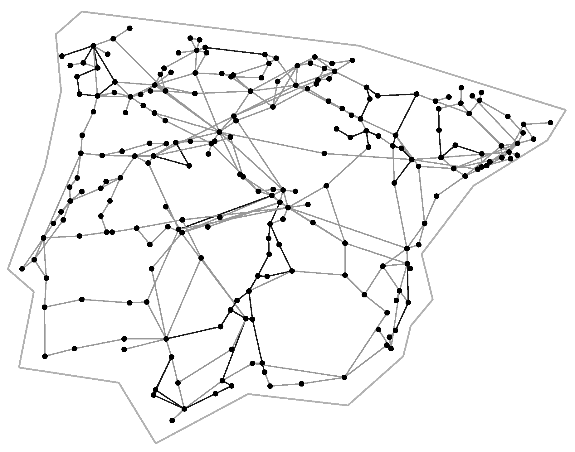
3.2. Iberian Peninsula Power System
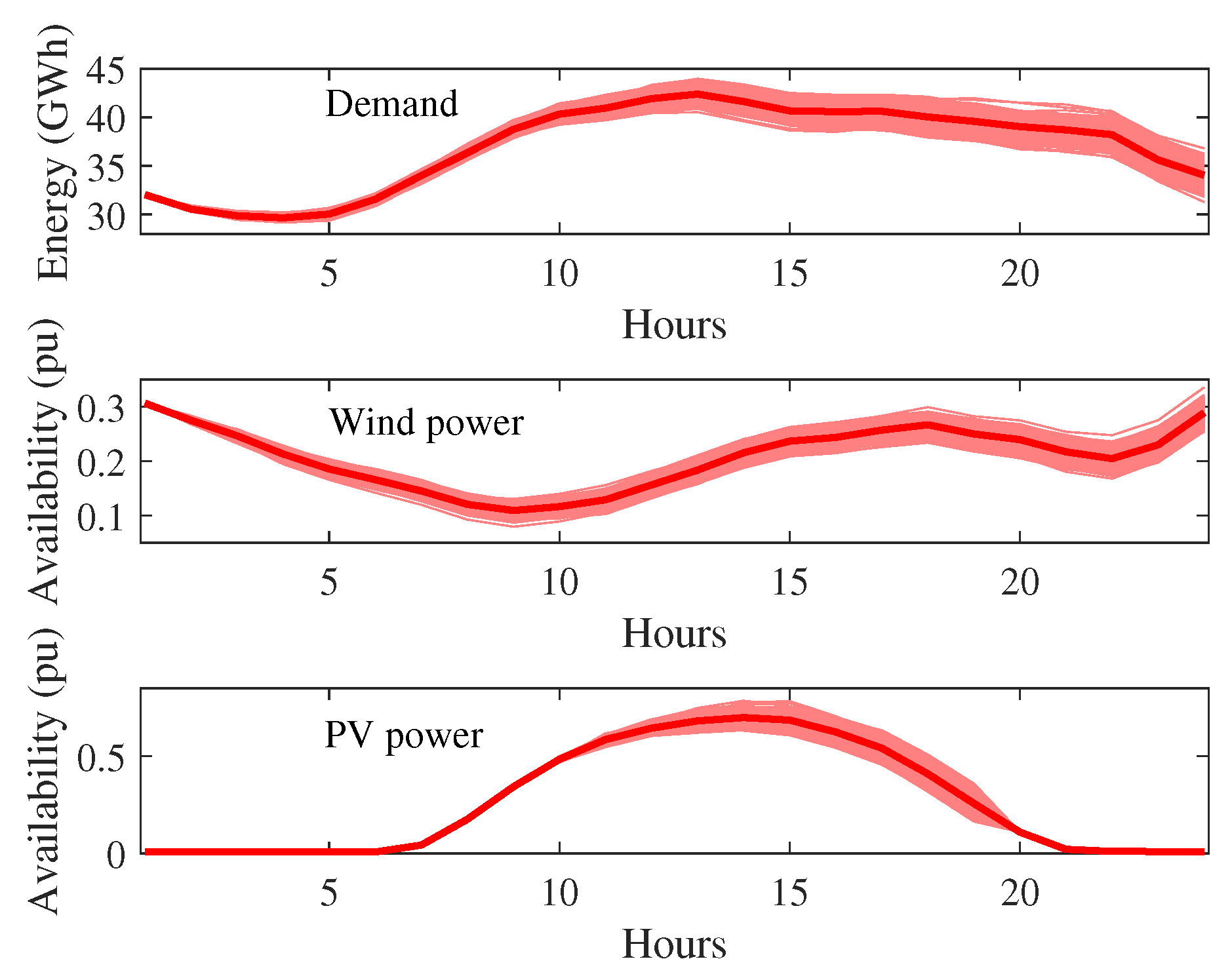
3.2.1. Input Data

A realistic case study based on the Iberian Peninsula power system has been solved to analyze the performance of problem (P1) for different values of the threshold probability α . The representation of this power system is based on the approximate model of the European Interconnected System reported in [29], and on the the available information in the annual reports published by the system operators of Spain [26] and Portugal [30]. This system comprises 226 buses and 390 transmission lines. The transmission network is depicted in Figure 2, where light and dark lines represent 400 and 220 kV lines, respectively. The detailed description of this system is provided in [25]. The installed capacity per generation technology is represented in Table 7. The solar photovoltaic (PV) capacity has been assigned to each bus according to the information provided in [26,30].
The target year considered in this case study is 2017. Consequently, the actual values of demand and wind and solar power outputs of that year are used. The operating costs of wind and solar photovoltaic (PV) power units are considered to be null, whereas the average operating costs of nuclear, coal, OCGT, CCGT and hydro units are 10, 48, 70, 60 and 58 €/MWh, respectively. All these data are based on reports from the US Energy Information Administration (EIA) [31] and the National Renewable Energy Laboratory (NREL) [32]. We assume that these operating costs are equal to the capacity offer prices submitted by the units in the day-ahead energy market. Up and down reserve capacity prices offered by generators are equal to 0.2 times the energy offer prices. It is considered that 3% of the total demand in each bus can participate in the reserve capacity market. The up and down reserve capacity prices offered by demands are equal to 30 €/MW. The minimum up and down times of nuclear, coal and CCGT units are equal to 24, 8 and 3 h, respectively. For the rest of technologies, minimum up and down times are equal to 1 h. The load shedding and forced wind spillage penalty costs are equal to €1000/MWh and €200/MWh, respectively.
As done in the previous case study, an out-of-sample analysis is carried out to model the balancing market and test the day-ahead energy and reserve schedule obtained from the proposed formulation. To do that, a different set of 500 scenarios is considered. We also consider that the deployment of up and down reserves by generating units is 1.1 and 0.85 times the energy price offers, respectively. The deployment of up and down reserves by flexible demands is 250 and 0 €/MWh, respectively. We assume that all committed units in the day-ahead energy market are able to deploy non-scheduled up and down spinning reserves. Non-scheduled up reserves are priced at 1.5 times the cost of the deployment of scheduled reserves, whereas down non-scheduled reserves prices are fixed to 0.

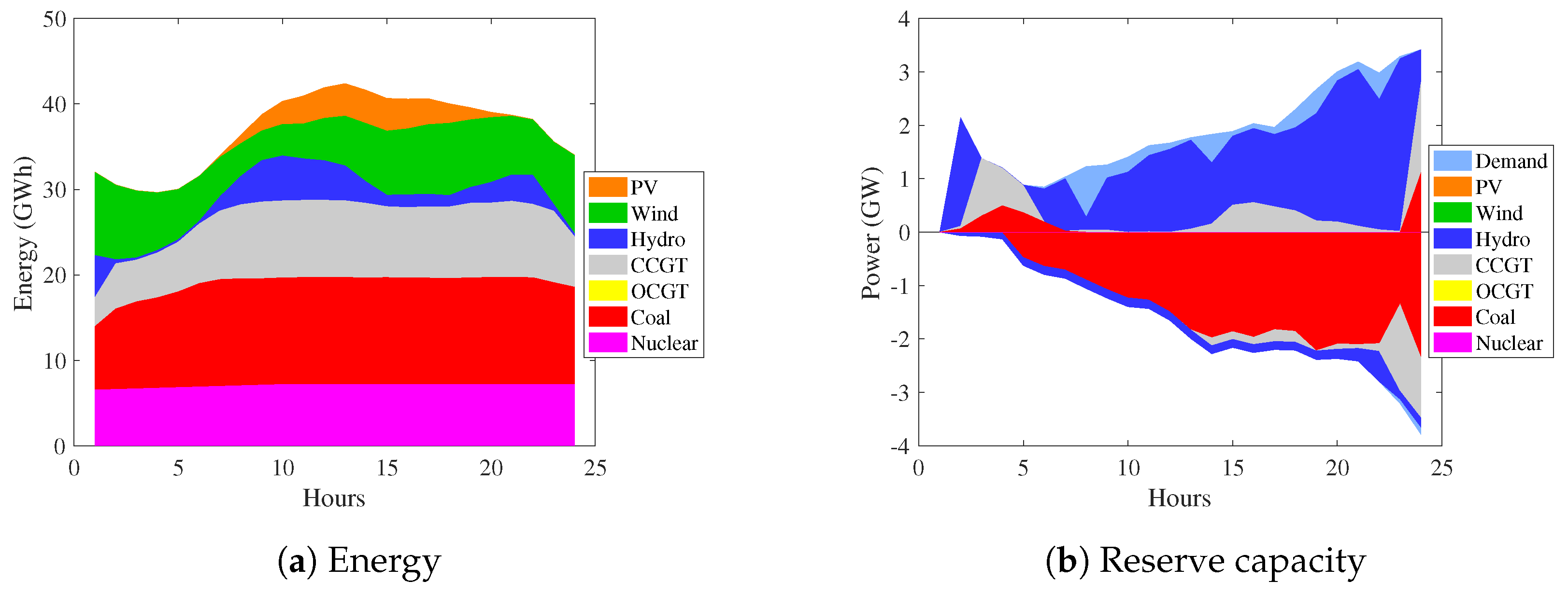
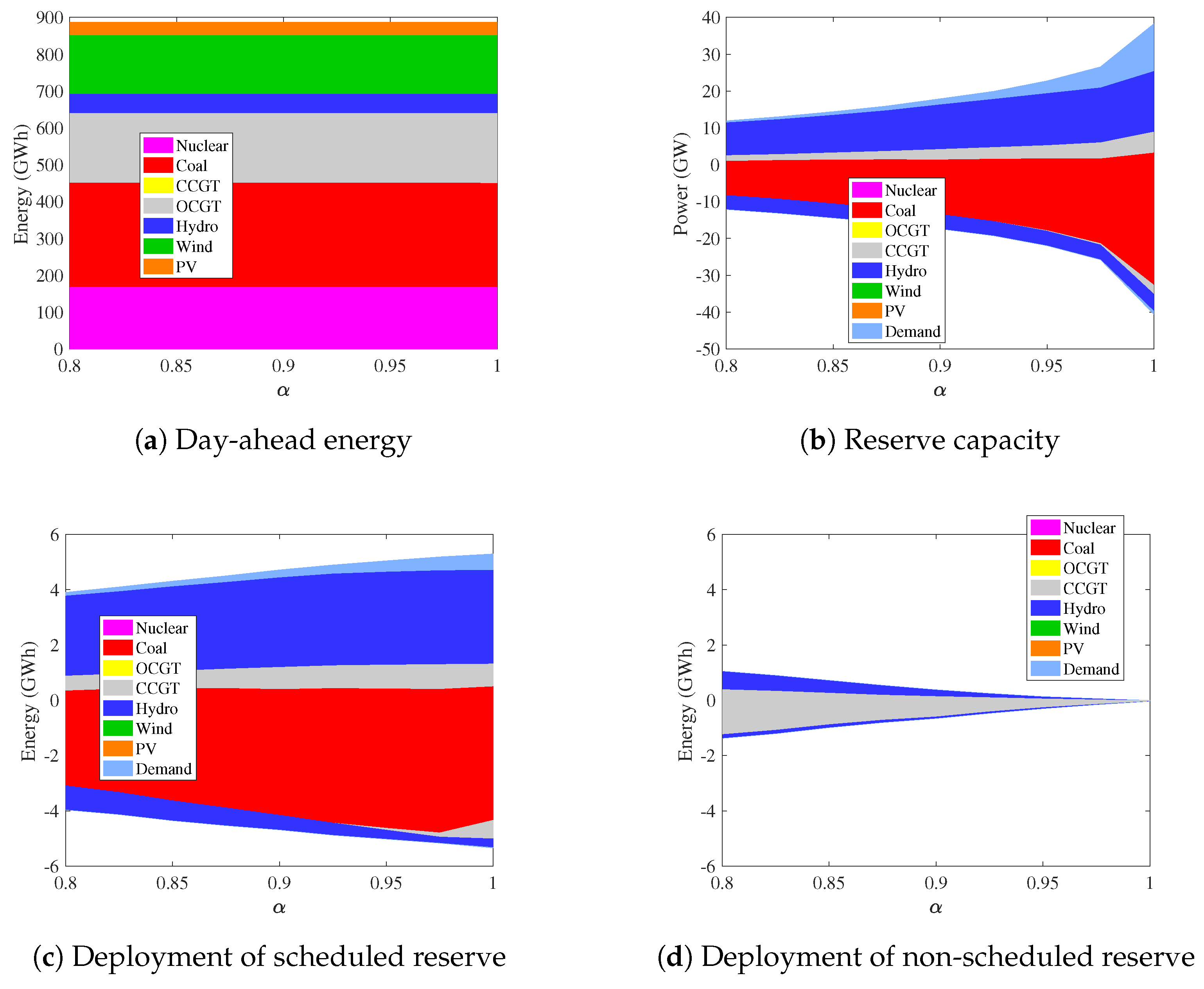
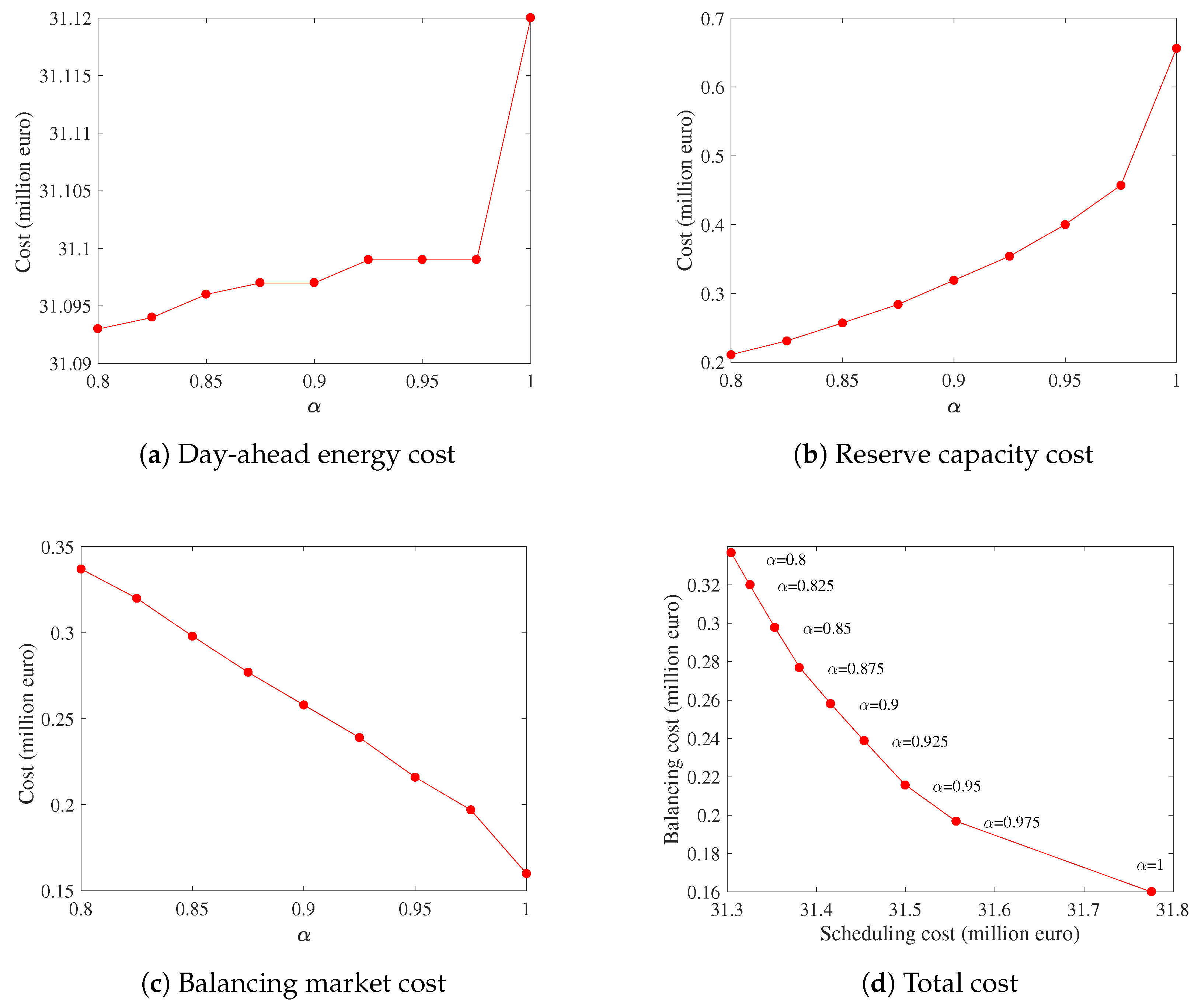
3.2.2. Day-Ahead Scheduling Results

In this section, the proposed formulation is applied to the 5th of July of 2017 in the Iberian Peninsula power system. To do that, a set of 500 scenarios of demand, wind and PV availability has been generated using the approach described in [25]. Figure 3 represents the resulting scenarios, where bold lines indicate the expected values of each series.
Figure 4 plots the resulting day-ahead scheduling obtained from solving the proposed formulation to the case study described previously. This problem has 208,343 constraints, and 189,121 and 3,312 continuous and binary variables, respectively. The solution time of this problem is 280 seconds.
Figure 4a shows that nuclear and coal technologies are used as base units, whereas hydro units participate as peak units. The scheduling of up and down reserve capacities depicted in Figure 4b are mostly provided by hydro and coal units, respectively. Please note that the demand participates providing up reserve in some periods.
Figure 5 represents the expected and maximum costs for the given day for different values of α . As described in Section 2, the threshold probability α is an indicator of the risk aversion faced by the system operator in the day-ahead scheduling. The expected cost is equal to the summation of the energy, reserve capacity and startup and shutdown costs plus the expected balancing market cost. Please note that the balancing market costs are calculated over the set of out-of-sample scenarios. The maximum cost is computed equivalently to the expected cost, but the expected balancing market cost is replaced by the cost associated with the scenario with higher balancing market cost. Figure 5 shows that the risk-aversion level only slightly affects the expected cost. The minimum expected cost, which is obtained for α = 0.975 , amounts to 36.34 million €, only 0.3% smaller than that obtained from considering the most risk-averse position, α = 1 . We can also observe that the maximum cost is highly dependent of the degree of risk aversion. For instance, the maximum cost for α = 1 is 17.6% less than the maximum cost attained for α = 0.8 .
Figure 6 plots the scheduling and deployment of energy and reserve for different values of α . In Figure 6a we observe that the day-ahead energy schedule remains quite stable with respect to α . However, Figure 6b shows that the scheduling of reserve capacity grows significantly as α increases. A high increment of the reserve capacity scheduled is observed for values of α greater than 0.95. As a consequence of the increment of the scheduling of the reserve capacity, we observe that the deployment of scheduled reserves shown in Figure 6c,d increases whereas the deployment of non-scheduled reserves reduces. In fact, we observe that non-scheduled reserves represent 25% of all deployed reserves for α = 0.8 , whereas they are negligible for α = 1 .
Figure 7 represents the day-ahead energy, reserve capacity and balancing costs as a function of α . Figure 7a,b show that the day-ahead energy and reserve capacity costs grow as α increases. The day-ahead energy and reserve capacity cost increments for α = 1 with respect to α = 0.8 are 0.05 and 218.12%, respectively. Please note that the reserve capacity cost only represents around 2% of the day-ahead energy cost. The increment of the scheduling of reserves decreases the deployment of non-scheduled reserves (see Figure 6d) which causes a decrement in the balancing market costs. In Figure 7c we observe that these costs are reduced 45.65% from α = 0.8 to α = 1 . Finally, Figure 7d represents the balancing cost versus the scheduling cost (day-ahead energy + reserve capacity cost) for different values of α . This figure shows that the relationship between scheduling and balancing costs is approximately linear for values of α comprised between 0.8 and 0.925. For larger values of α , the cost in the balancing market is reduced due to a higher increment of the scheduling cost, which leads to a higher total cost, as previously shown in Figure 5.

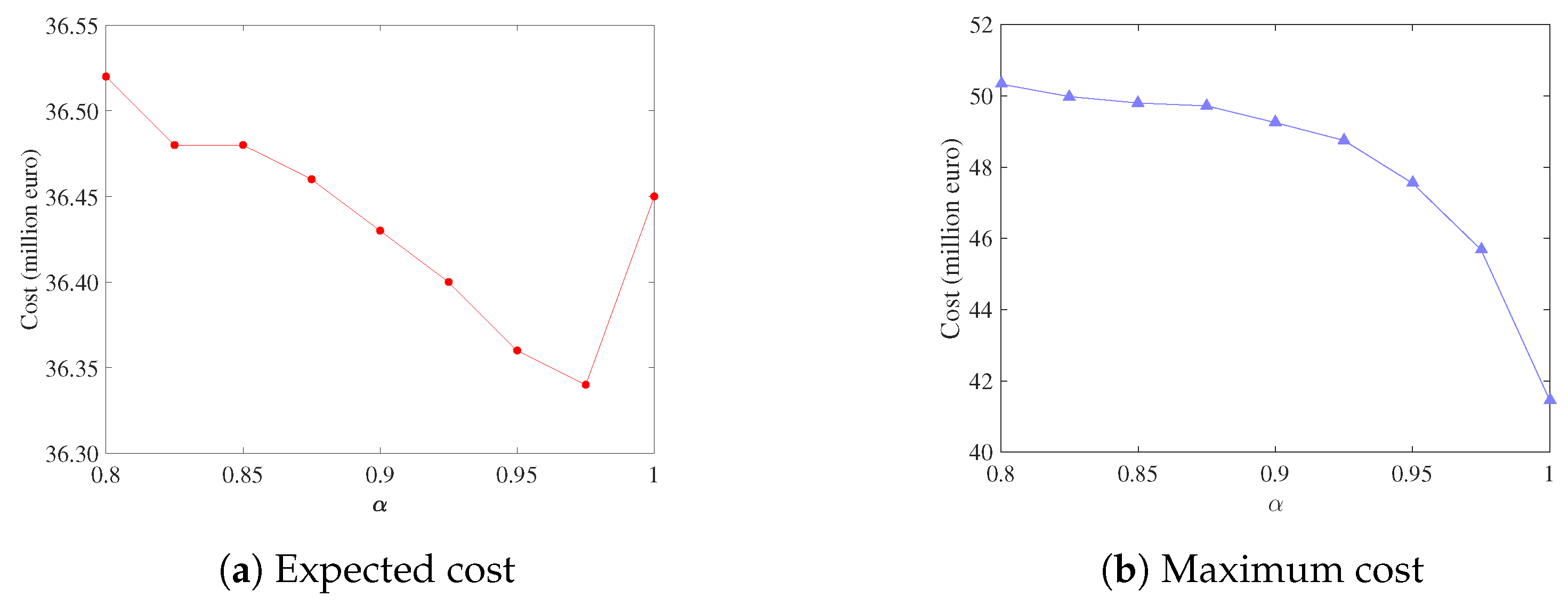
3.2.3. System Operation for One Year

Finally, to test the performance of the proposed formulation in a longer period of time, the proposed day-ahead scheduling procedure has been applied iteratively for each of the 365 days of 2017. For every single day, 500 scenarios of demand, wind and solar PV power availabilities are generated. To analyze the performance of the obtained day-ahead scheduling, a single realization of the uncertain parameters has been randomly generated for modeling the operation of the balancing market in each day.
Considering this, four different cases are solved:
  • α = 0.95 . The proposed formulation is used for α = 0.95 .
  • α = 1.00 . The proposed formulation is used for α = 1 .
  • RES 1 . The reserve requirements are computed based on the actual practices of the Spanish power system operator [22]. This way, constraints (34)–(41) are replaced by the following ones:
    g G D b g t G , U + d b d t D , U 10 d L d t DA + 150 2 150 + 0.02 d L d t DA + 0.13 g G I U g t DA P max , g C , t
    g G D b g t G , D + d b d t D , D 10 d L d t DA + 150 2 150 + 0.02 d L d t DA , t
  • RES 2 . The reserve requirements are set based on the (3 + 5)% policy devised by NREL in [23], which requires the system to carry hourly up and down spinning reserve greater than 3% of hourly forecast demand plus 5% of hourly forecast wind and PV power. Therefore, constraints (34)–(41) are replaced by:
    g G D b g t G , U + d b d t D , U 0.03 d L d t DA + 0.05 g G I U g t DA P max , g C , t
    g G D b g t G , D + d b d t D , D 0.03 d L d t DA + 0.05 g G I U g t DA P max , g C , t
The most relevant results obtained in terms of costs and scheduled and deployed energy are provided in Table 8. This table shows that the proposed formulation with α = 0.95 and α = 1 attains the lowest total costs.
The obtained startup and shutdown costs for the different formulations are quite similar. It should be noted that the greatest cycling of thermal units occurs in RES 2 case, resulting in larger startup and shutdown costs. There are no significant differences among the day-ahead energy (DA energy) costs obtained by the different formulations. The largest cost is obtained in α = 1 case, which is only 0.5% greater than the smallest cost (RES 2 case). However, the scheduling of up and down reserve capacities (DA Res. up and DA Res. down) is quite different among the four cases. For instance, the schedules of up and down reserves in α = 0.95 case are 37.7% and 44.8% less than in α = 1 case, respectively. It is also observed that, as established by constraints (44) and (45), the quantities scheduled of up and down reserve capacities are identical in RES 2 case. The greatest quantity of up reserve capacity is scheduled in RES 1 case. Please note that the average price for the up reserve capacity in this case is 11.4 €/MWh, which is 8% less than that in α = 1 case. This result is quite relevant and is explained by the fact that, in contrast with the proposed formulation, the reserve capacity needs in RES 1 case are computed without considering the transmission network in constraints (42) and (43). In this manner, the cheapest up and down reserve capacity offers are selected without considering the location of the generating units in the network. Please note that this fact applies also for the RES 2 case. The effect of this can be observed in the deployments of scheduled (Bal Dep. up and Bal Dep. down) and non-scheduled (Bal NoSch. up and Bal NoSch. down) reserves. It is observed that the deployment of non-scheduled reserves in RES 1 and RES 2 cases is significantly larger than in α = 0.95 and α = 1 cases, which result in high balancing costs. From this result it can be concluded that considering the network topology is very important in order to effectively establish the reserve capacity needs of the system. Finally, it is also observed that the highest expected intermittent power spillage (Int. spillage) and unserved demand (Uns. demand) are obtained by RES 1 and RES 2 cases. On the contrary, the proposed formulation with α = 1 obtains the smallest intermittent power spillage and load shed.

4. Summary and Conclusions

This paper proposes a practical unit commitment formulation to co-optimize the day-ahead energy and spinning reserve capacity scheduling. The proposed formulation uses an estimation of the positive and negative deviations of the net load in the balancing market with respect to the day-ahead market quantities. These deviations are computed using a probabilistic procedure that allows to incorporate the risk-aversion preferences of the system operator. The main advantage of the proposed formulation is that it requires a significant smaller number of variables that other approaches based on stochastic programming models whose computational complexity is highly dependent on the considered number of scenarios. The numerical results show that the proposed formulation attains solution times smaller than other deterministic procedures and allows effectively to include a tradeoff between day-ahead scheduling and balancing dispatching costs. The results also suggest that the proposed technique would be able to provide energy and reserve capacity schedules comparable with those obtained by stochastic programming approaches, with significant reductions in computation times. The procedure enables the system operator to manage the risk of having to resort to non-scheduled reserves and wind spillages in the real-time operation. This flexibility could lead to important savings regarding to operation costs. Finally, it is shown that the proposed model may outperform in terms of costs actual practices of power system operators.

Author Contributions

M.C. proposed the core idea, performed the simulations and exported the results. M.C., R.Z.-M. and R.D. contributed to the design of the models and the writing of this manuscript.

Funding

This work has been funded and supported by the Ministry of Economy and Competitiveness of Spain under Project DPI2015-71280-R MINECO/FEDER, UE.

Conflicts of Interest

The authors declare no conflict of interest.

Appendix A. Stochastic Unit Commitment Formulation

The formulation of the stochastic unit commitment problem described in Section 3.1 is:
Problem ( P 2 ) Minimize Θ 2 Objective function ( 10 )
Subject to:
(Day-ahead market constraints)
Constraints (11)–(33)
(Balancing market constraints)
{ s max , g t B s g t ω B , g G I , t
p max , n t UD p n t ω UD , n , t
p g t ω B = p g t DA + r g t ω G , U r g t ω G , D , g G D , t
p g t ω B + s g t ω B = U g t ω B P max , g G , g G I , t
s g t ω B 0 , g G I , t
0 r g t ω G , U b g t G , U , g G D , t
0 r g t ω G , D b g t G , D , g G D , t
0 r d t ω D , U b d t D , U , d , t
0 r d t ω D , D b d t D , D , d , t
p t ω L , B = 1 X θ O ( ) t ω B θ F ( ) t ω B , , t
P max , L p t ω L , B P max , L , , t
g G n D r g t ω G , U r g t ω G , D + d D n r d t ω D , U r d t ω D , D + g G n I p g t ω B p g t DA L n O p t ω L , B p t L , DA + L n F p t ω L , B p t L , DA + p n t ω UD = d D n L d t ω B L d t DA , n , t } , ω
Auxiliary constraints (A1) and (A2) compute the maximum power spillage and unserved demand that are penalized in the objective function (10). Constraints (A3) and (A4) compute the power outputs of dispatchable and intermittent units in the balancing market. The power output of a dispatchable unit is equal to the energy scheduled in the day-ahead market plus the deployed up reserve minus the deployed down reserve. The power output of an intermittent unit in the balancing market is bounded by the availability factor U g t ω B . Constraints (A5) establish the positivity of the intermittent production spillage in the balancing market. The deployed up and down reserves of generating units and demands are bounded by the up and down reserve schedules by constraints (A6)–(A9). The dc power flows in the transmission lines are formulated and limited by constraints (A10) and (A11), respectively. Finally, constraints (A12) ensure the balance for the power deviations in the balancing market.

References

  1. International Energy Agency. 2017. Available online: http://www.iea.org (accessed on 7 May 2018).
  2. Gooi, H.B.; Mendes, D.P.; Bell, K.R.W.; Kirschen, D.S. Optimal scheduling of spinning reserve. IEEE Trans. Power Syst. 1999, 14, 1485–1492. [Google Scholar] [CrossRef]
  3. Bouffard, F.; Galiana, F.D. Stochastic security for operations planning with significant wind power generation. IEEE Trans. Power Syst. 2008, 23, 306–316. [Google Scholar] [CrossRef]
  4. Ortega-Vazquez, M.A.; Kirschen, D.S. Estimating the spinning reserve requirements in systems with significant wind power generation penetration. IEEE Trans. Power Syst. 2009, 24, 114–124. [Google Scholar] [CrossRef]
  5. Pritchard, G.; Zakeri, G.; Philpott, A. A single-settlement, energy-only electric power market for unpredictable and intermittent participants. Oper. Res. 2010, 58, 1210–1219. [Google Scholar] [CrossRef]
  6. Papavasiliou, A.; Oren, S.S.; O’Neill, R.P. Reserve requirements for wind power integration: A scenario-based stochastic programming framework. IEEE Trans. Power Syst. 2011, 26, 2197–2206. [Google Scholar] [CrossRef]
  7. Bertsimas, D.; Litvinov, E.; Sun, X.A.; Zhao, J.; Zheng, T. Adaptive Robust Optimization for the Security Constrained Unit Commitment Problem. IEEE Trans. Power Syst. 2013, 28, 52–63. [Google Scholar] [CrossRef] [Green Version]
  8. Morales, J.M.; Zugno, M.; Pineda, S.; Pinson, P. Redefining the merit order of stochastic generation in forward markets. IEEE Trans. Power Syst. 2014, 29, 992–993. [Google Scholar] [CrossRef]
  9. Domínguez, R.; Conejo, A.J.; Carrión, M. Operation of a fully renewable electric energy system with CSP plants. Appl. Energy 2014, 119, 417–430. [Google Scholar] [CrossRef]
  10. Hytowitz, R.B.; Hedman, K.W. Managing solar uncertainty in microgrid systems with stochastic unit commitment. Electr. Power Syst. Res. 2015, 119, 111–118. [Google Scholar] [CrossRef]
  11. Marneris, I.G.; Biskas, P.N.; Bakirtzis, A.G. Stochastic and deterministic unit commitment considering uncertainty and variability reserves for high renewable integration. Energies 2017, 10, 140. [Google Scholar] [CrossRef]
  12. Jo, K.-H.; Kim, M.-K. Stochastic unit commitment based on multi-scenario tree method considering uncertainty. Energies 2018, 11, 740. [Google Scholar] [CrossRef]
  13. Zugno, M.; Conejo, A.J. A robust optimization approach to energy and reserve dispatch in electricity markets. Eur. J. Oper. Res. 2015, 247, 659–671. [Google Scholar] [CrossRef] [Green Version]
  14. Zheng, Q.P.; Wang, J.; Liu, A.L. Stochastic Optimization for Unit Commitment—A Review. IEEE Trans. Power Syst. 2015, 30, 1913–1924. [Google Scholar] [CrossRef]
  15. Alqurashi, A.; Etemadi, A.H.; Khodaei, A. Treatment of uncertainty for next generation power systems: State-of-the-art in stochastic optimization. Electr. Power Syst. Res. 2016, 141, 233–245. [Google Scholar] [CrossRef]
  16. LaBove, G.L.; Al-Abdullah, Y.M.; Hedman, K.W. Scaling Issues in Day-Ahead Formulations of Stocashtic Unit Commitment. In Proceedings of the 2015 North American Power Symposium (NAPS), Charlotte, NC, USA, 4–6 October 2015; pp. 1–6. [Google Scholar]
  17. Gröwe-Kuska, N.; Heitsch, H.; Römisch, W. Scenario reduction and scenario tree construction for power management problems. In Proceedings of the 2003 IEEE Bologna Power Tech Conference, Bologna, Italy, 23–26 June 2003. [Google Scholar] [Green Version]
  18. Carrión, M.; Arroyo, J.M. A Computationally Efficient Mixed-Integer Linear Formulation for the Thermal Unit Commitment Problem. IEEE Trans. Power Syst. 2006, 21, 1371–1378. [Google Scholar] [CrossRef]
  19. Anjos, M. Recent progress in modeling unit commitment problems. In Springer Proceedings in Mathematics and Statistics; Springer: New York, NY, USA, 2013; Volume 62, pp. 3–29. [Google Scholar]
  20. Cancelo, J.R.; Espasa, A.; Grafe, R. Forecasting the electricity load from one day to one week ahead for Spanish system operator. Int. J. Forecast. 2008, 24, 588–602. [Google Scholar] [CrossRef] [Green Version]
  21. Wind Generation Forecasting at REE. Available online: http://www.ieawindforecasting.dk/publications (accessed on 7 May 2018).
  22. Lobato, E.; Egido, I.; Rouco, L.; López, G. An overview of ancillary services in Spain. Electr. Power Syst. Res. 2008, 78, 515–523. [Google Scholar] [CrossRef]
  23. Western Wind and Solar Integration Study; Technical Report; National Renewable Energy Laboratory: Golden, CO, USA, May 2010. Available online: https://goo.gl/NvUBK8 (accessed on 7 May 2018).
  24. Grigg, C.; Wong, P.; Albrecht, P.; Allan, R.; Bhavaraju, M.; Billinton, R.; Chen, Q.; Fong, C.; Haddad, S.; Kuruganty, S.; et al. The IEEE reliability test system-1996. IEEE Trans. Power Syst. 1999, 143, 1010–1020. [Google Scholar] [CrossRef]
  25. Carrión, M.; Zárate-Miñano, R. Operation of intermittent-dominated power systems with a significant penetration of plug-in electric vehicles. Energy 2015, 90, 827–835. [Google Scholar] [CrossRef]
  26. Spanish Network Operator (Red Eléctrica de España). Available online: http://www.ree.es (accessed on 7 May 2018).
  27. The IBM CPLEX. Available online: http://www-01.ibm.com/software/commerce/optimization/cplex-optimizer/ (accessed on 7 May 2018).
  28. Rosenthal, R.E. GAMS—A Users Guide; GAMS Development Company: Washington, DC, USA, 2008. [Google Scholar]
  29. Zhou, Q.; Bialek, J.W. Approximate model of European interconnected system as a benchmark system to study effects of cross-border trades. IEEE Trans. Power Syst. 2005, 20, 782–788. [Google Scholar] [CrossRef]
  30. Portuguish Network Operator (Redes Energéticas Nacionais). Available online: http://www.ren.pt (accessed on 7 May 2018).
  31. US Energy Information Administration Updated Capital Cost-Estimates for Utility Scale Electricity Generating Plants. April 2013. Available online: http://www.eia.gov/ (accessed on 8 May 2012).
  32. Hand, M.M. (Ed.) Renewable Electricity Futures Study; 4 vols., NREL/TP-6A20-52409; National Renewable Energy Laboratory: Golden, CO, USA, 2012. Available online: https://www.nrel.gov/analysis/re-futures.html (accessed on 7 May 2018).
Figure 1. Scenarios for electricity demand and wind availability.
Energies 11 01939 g001
Figure 2. Iberian Peninsula transmission network.
Energies 11 01939 g002
Figure 3. Demand, wind and PV availability scenarios for 5th of July of 2017.
Energies 11 01939 g003
Figure 4. Day-ahead energy and reserve capacity scheduling.
Energies 11 01939 g004
Figure 5. Maximum and expected total cost with respect to α .
Energies 11 01939 g005
Figure 6. Scheduling and deployment of energy and reserve with respect to α .
Energies 11 01939 g006
Figure 7. Total cost with respect to α .
Energies 11 01939 g007
Table 1. Characteristics of the generating units.
TechnologyBus P max , g G P min , g G P up , g G / P dw , g G U g T / D g T C g DA C g SU
(MW)(MW)(MW)(h)(€/MWh)(k€)
Nuclear18, 214001602012096.0
Coal15, 16,1553146.583239.7
23 (2)
OCGT2 (2)200101501.0
7 (2)1000501505.0
13 (3)197098.51509.8
CCGT15 (5)122.44.83401.2
1 (2)20483402.0
1 (2), 2 (2)7615.230.43407.6
Hydro22 (5)505501450.5
Wind22, 7 (2)4500-000.0
136000-000.0
2310500-000.0
Table 2. Computational size and computing time.
ItemDUCSUCPF
# binary variables ( × 10 3 ):0.770.770.77
# continuous variables ( × 10 3 ):208.54202.0612.36
# constraints ( × 10 3 ):314.49301.8218.96
Computing time (s):5857314
Table 3. Expected costs.
P Tot W FormulationDA-ESUSDDA-RBTotal
(GW)(k€)(k€)(k€)(k€)(k€)(k€)
1DUC620.24115.710.212.987.61746.75
SUC620.24115.710.213.037.48746.67
PF ( α = 0.80 ) 620.24115.710.210.7811.78748.72
PF ( α = 0.90 ) 620.24115.710.211.209.79747.15
PF ( α = 1.00 ) 620.24115.710.213.127.46746.74
2DUC511.9997.290.292.8514.85627.29
SUC514.2397.290.293.226.94621.97
PF ( α = 0.80 ) 512.6497.290.290.9211.97623.12
PF ( α = 0.90 ) 512.7497.290.291.3710.14621.84
PF ( α = 1.00 ) 513.0798.890.363.356.60622.27
3DUC427.1366.550.601.92114.18610.39
SUC447.6076.070.613.749.50537.52
PF ( α = 0.80 ) 427.4870.560.591.0845.54545.23
PF ( α = 0.90 ) 428.7271.820.591.5834.81537.52
PF ( α = 1.00 ) 433.5375.570.513.9626.33539.91
SU: Startup costs; SD: Shutdown costs; DA-E: Day-ahead energy costs; DA-R: Reserve capacity costs; B: Balancing costs (out-of-sample).
Table 4. Expected balancing costs.
P Tot W FormulationEnergyUns. DemandWind SpillageTotal
(GW)(k€)(k€)(k€)(k€)
1DUC7.610.000.007.61
SUC7.480.000.007.48
PF ( α = 0.80 ) 11.780.000.0011.78
PF ( α = 0.90 ) 9.790.000.009.79
PF ( α = 1.00 ) 7.460.000.007.46
2DUC8.206.650.0014.85
SUC6.890.050.006.94
PF ( α = 0.80 ) 11.910.050.0111.97
PF ( α = 0.90 ) 10.080.050.0110.14
PF ( α = 1.00 ) 6.600.000.006.60
3DUC4.7683.1626.25114.18
SUC8.580.000.929.50
PF ( α = 0.80 ) 9.9312.9222.6945.54
PF ( α = 0.90 ) 7.954.1622.6934.81
PF ( α = 1.00 ) 3.670.0022.6726.33
Table 5. Day-ahead energy scheduling (GWh).
P Tot W (GW)FormulationNuclearCoalOCGTCCGTHydroWind
1DUC18.846.335.474.053.342.69
SUC18.846.335.474.053.342.69
PF ( α = 0.80 ) 18.846.335.474.053.342.69
PF ( α = 0.90 ) 18.846.335.474.053.342.69
PF ( α = 1.00 ) 18.846.335.474.053.342.69
2DUC18.846.303.803.552.855.37
SUC18.846.243.813.492.975.37
PF ( α = 0.80 ) 18.846.303.733.552.925.37
PF ( α = 0.90 ) 18.846.303.753.542.925.37
PF ( α = 1.00 ) 18.836.243.763.712.805.37
3DUC18.844.243.093.682.947.93
SUC18.294.243.653.682.798.06
PF ( α = 0.80 ) 18.844.243.033.912.837.88
PF ( α = 0.90 ) 18.844.233.043.932.827.85
PF ( α = 1.00 ) 18.834.243.343.572.997.75
Table 6. Up/Down spinning reserve scheduling (GW).
P Tot W (GW)FormulationCoalOCGTCCGTHydroTotal
1DUC0.0/0.81.5/0.10.1/0.30.4/0.92.0/ 2.1
SUC0.0/0.81.5/0.10.1/0.30.4/0.92.1/ 2.1
PF ( α = 0.80 ) 0.0/0.40.3/0.00.0/0.00.2/0.10.6/0.6
PF ( α = 0.90 ) 0.0/0.60.6/0.00.0/0.10.3/0.20.9/0.9
PF ( α = 1.00 ) 0.0/0.81.6/0.10.1/0.30.4/0.92.1/ 2.1
2DUC0.1/ 1.01.3/0.10.1/0.30.4/0.91.9/ 2.3
SUC0.1/ 1.00.9/0.10.1/0.31.2/ 1.02.3/ 2.4
PF ( α = 0.80 ) 0.0/0.50.3/0.00.1/0.10.3/0.10.7/0.7
PF ( α = 0.90 ) 0.0/0.60.5/0.00.1/0.10.4/0.31.0/ 1.0
PF ( α = 1.00 ) 0.1/ 1.01.3/0.20.2/0.30.8/ 1.02.4/ 2.4
3DUC0.0/0.90.2/0.30.2/0.30.5/0.80.9/ 2.4
SUC0.0/0.91.5/0.50.2/0.30.9/0.82.5/ 2.6
PF ( α = 0.80 ) 0.0/0.50.1/0.10.1/0.10.6/0.20.8/0.9
PF ( α = 0.90 ) 0.0/0.60.2/0.10.2/0.10.8/0.41.2/ 1.2
PF ( α = 1.00 ) 0.0/ 1.01.5/0.40.2/0.31.0/ 1.12.8/ 2.7
Table 7. Installed capacity of generating technologies.
ItemNuclearCoalOCGTCCGTHydroWindPVTotal
Capacity (GW)7.112.55.531.921.131.75.6118.4
Number of units (#)51910267790226593
Table 8. Annual results.
Expected Cost (Millions €)Expected Energy (GWh)
α = 0.95 α = 1.00       RES 1     RES 2 α = 0.95 α = 1.00       RES 1     RES 2
Total 10,389.110,527.011,646.411,536.0298,939.4298,939.4298,939.4298,939.4
Startup90.793.8100.3121.0----
Coal22.922.320.125.8----
OCGT1.63.03.24.9----
CCGT66.268.576.990.4----
Shutdown35.536.538.446.3----
Coal9.19.17.710.2----
OCGT0.00.00.00.0----
CCGT26.427.430.736.1----
DA Energy9496.49517.39489.79471.6298,925.2298,936.1298,898.7298,872.7
Nuclear612.6612.0613.3612.661,257.461,192.761,330.661,264.4
Coal4516.04493.94518.04531.389,328.488,892.589,363.089,608.2
OCGT0.73.84.65.29.160.369.875.1
CCGT2954.32980.92902.22876.749,400.849,721.248,732.548,451.5
Hydro1412.81426.71451.61445.823,765.323,911.624,258.824,338.7
Wind0.00.00.00.065,338.165,331.865,318.265,308.8
PV0.00.00.00.09826.09826.09826.09826.0
DA Res. up136.5225.2225.0144.311,363.418,231.319,710.312,728.5
Coal17.820.426.018.31599.21816.62509.41768.4
OCGT0.00.10.10.42.04.97.626.3
CCGT25.643.238.527.02026.33360.13206.52247.6
Hydro89.4157.5158.096.57377.312,647.113,746.48468.4
Demand3.64.02.42.2358.6402.5240.4217.7
DA Res. down59.4123.376.1102.77684.513,912.69933.512,728.5
Coal53.794.673.397.15851.710,014.68291.810,816.3
OCGT0.00.00.00.30.00.00.021.6
CCGT1.312.11.41.4107.81049.5114.6116.4
Hydro2.912.80.62.51570.82471.81445.61632.1
Demand1.53.80.81.4154.2376.781.4142.0
Bal Dep. up321.3322.3345.8311.84216.14293.74598.44152.0
Coal42.843.122.222.4695.5690.1391.7398.0
OCGT0.00.00.20.70.10.62.08.4
CCGT53.763.043.839.2770.1899.3677.5601.8
Hydro212.6211.9263.2226.32689.82682.73444.83028.1
Demand0.04.216.523.160.621.182.4115.5
Bal Dep. down−59.8−72.6−57.7−63.81509.31609.61657.51763.9
Coal−51.6−41.6−55.9−59.41283.6978.71488.91552.1
OCGT0.00.00.0−0.10.00.00.01.5
CCGT−2.3−13.4−1.2−0.945.4270.624.816.7
Hydro−5.9−17.6−0.5−3.4179.8359.8143.3193.0
Demand0.00.00.00.044.348.050.562.2
Bal NoSch. up8.80.353.784.177.52.8402.8662.5
Coal0.00.00.00.00.00.00.00.0
OCGT0.00.00.00.30.00.00.02.6
CCGT5.20.223.744.148.72.3211.7395.8
Hydro3.60.130.039.728.90.5191.1264.1
Bal NoSch. dw0.00.00.00.092.23.5707.6543.0
Coal0.00.00.00.00.00.00.00.0
OCGT0.00.00.00.00.00.00.10.1
CCGT0.00.00.00.068.02.4582.2441.8
Hydro0.00.00.00.024.21.1125.3101.1
Int. spillage292.5280.41147.91000.71462.51402.15739.65003.6
Uns. demand7.80.5227.2317.37.80.5227.2317.3

