Article

A Stochastic Model Predictive Control Approach for Joint Operational Scheduling and Hourly Reconfiguration of Distribution Systems

by
Saeid Esmaeili
1,
Amjad Anvari-Moghaddam
2,
Shahram Jadid
1,* and
Josep M. Guerrero
2
1
Department of Electrical Engineering, Iran University of Science and Technology, Tehran 16846-13114, Iran
2
Department of Energy Technology, Aalborg University, 9220 Aalborg East, Denmark
*
Author to whom correspondence should be addressed.
Energies 2018, 11(7), 1884; https://doi.org/10.3390/en11071884
Submission received: 20 May 2018 / Revised: 19 June 2018 / Accepted: 20 June 2018 / Published: 19 July 2018

Abstract

:
Due to the recent developments in the practical implementation of remotely controlled switches (RCSs) in the smart distribution system infrastructure, distribution system operators face operational challenges in the hourly reconfigurable environment. This paper develops a stochastic Model Predictive Control (MPC) framework for operational scheduling of distribution systems with dynamic and adaptive hourly reconfiguration. The effect of coordinated integration of energy storage systems and demand response programs through hourly reconfiguration on the total costs (including cost of total loss, switching cost, cost of bilateral contract with power generation owners and responsive loads, and cost of exchanging power with the wholesale market) is investigated. A novel Switching Index (SI) based on the RCS ages and critical points in the network along with the maximum number of switching actions is introduced. Due to nonlinear nature of the problem and several existing binary variables, it is basically considered as a Mixed Integer Non-Linear Programming (MINLP) problem, which is transformed into a Mixed Integer Linear Programming (MILP) problem. The satisfactory performance of the proposed model is demonstrated through its application on a modified IEEE 33-bus distribution system.

1. Introduction

Due to the clean and sustainable nature of wind and solar energy resources, the future electricity distribution sector is envisioned to include a higher penetration of Renewable Energy Sources (RESs). The intermittent natural behavior of RESs may endanger the security and reliability of the power system. In [1,2], the Energy Storage Systems (ESSs) were implemented in the distribution system as a suitable solution for compensating these unexpected power fluctuations. In [3], a stochastic energy management system including RESs was proposed. It was demonstrated that by utilizing the ESSs the total expected cost of the distribution system is reduced and the fluctuations of RESs are smoothed out in different time scales. Generally, distribution systems have included various deployment of ESS technologies, such as battery ESSs, flow-battery ESSs, hydrogen-based fuel-cell ESSs, and fly wheel ESSs [4,5].
The second addressed solution in the literature to cope with the intermittency of RESs in short-term scheduling of distribution system is implementation of the Demand Response (DR) programs. According to the party that initiates the demand reduction action, market-driven actions or utility-driven actions, they are categorized into the price-based and incentive-based programs. In [6], a stochastic model scheduling of islanded microgrid with price-based DR actions is proposed. In this model, the expected profit of microgrid is maximized and the total customers’ payments are minimized, where in [7], optimal operational scheduling of a grid-connected microgrids has been developed using DR to mitigate the effect of uncertainties related to RESs. A stochastic programming model has been proposed in [8] to minimize the operating costs and emissions in a smart microgrid. The results demonstrate that the curtailed power related to Responsive Loads (RLs) participation are able not only to meet the plausible shortage of committed energy due to the uncertainties, but also to reduce the total operation costs. A conceptual study on a prosumer-based virtual power plant architecture considering DR programs is presented in [9]. In [10], by implementing a dynamic reconfiguration in the distribution system, a viable flexibility option has been provided to deal with the stochastic problem. A Mixed Integer Linear Programming (MILP) problem has been proposed to minimize the total operation costs. Distribution system reconfiguration is realized by the process of changing the topology of the network using the existing tie switches and sectionalizing switches to meet operator’s objectives.
Recently, the development in the practical implementation of information and communication technology infrastructure, sensors and control systems in smart distribution systems has been impressive. In this regard, the widespread operation of Remotely Controlled Switches (RCSs) in the smart distribution system infrastructure can provide a new operational opportunity for Distribution System Operators (DSOs). By introducing these switches, in addition to long-term reconfiguration plans (seasonal, annual) which has been discussed in [11,12,13], hourly (or generally a more frequent) reconfiguration can also be utilized for short-term scheduling of distribution systems. In [14], residential, commercial and industrial loads in summer/winter for weekday/weekend scenarios are considered for reconfiguration studies. In this paper, genetic algorithm is utilized to determine the optimal configuration of the power grid feeders with the objective of minimizing the line losses in the system. In [15], a bi-level scheduling problem is provided for short term operation of renewable energy resources in an active distribution system. In the first level, the amount of power purchased from the upstream grid and the state of distributed generations are determined, and in the second level, real-time scheduling in presence of hourly reconfiguration is proposed. In order to guarantee the acceptable life-time of RCSs, switching cost as an objective function and the maximum number of switching action as a constraint should be considered in the hourly reconfiguration of distribution systems, which are not considered in [14,15]. Nafisi, et al. [16] investigated hourly reconfiguration of the Sirjan 20 kV distribution system using a discrete genetic algorithm. In their paper, the objective function is considered as minimizing the switching cost and power system losses. Besides, constraints on bus voltages are added to the objective function in terms of a penalty factor. It is shown that by implementing hourly reconfiguration in a micro-grid even by considering the switching costs, total operation cost would decrease significantly. By increasing dispatchable and non-dispatchable power generation units’ penetration and RLs in smart distribution system, there is a need for a third party between them and the wholesale market [17,18]. This task can be performed by DSO who deals with Distribution Management System (DMS) to determine optimal set-points for power generation units and RLs according to the corresponding objective functions. In [19], an energy management system for distributed generations and RLs is presented considering the hourly reconfiguration. It should be mentioned that due to the nonlinear nature of the reconfiguration problem and several existing binary variables, it is basically considered as a Mixed Integer Non-Linear Programming (MINLP) problem. Because of the complicated mathematical formulations to solve MINLP problems in a reasonable time, heuristic methods are mainly utilized in [11,12,13,14,15,16,17,18,19] for problem solving. It is noteworthy to say that the weak point in heuristic solutions is failure to guarantee the optimality of the final solution.
Although utilization of ESSs, DR programs, and network reconfiguration can mitigate the intermittency of RESs, the stochastic optimization approaches have also been proposed in the literature to cope with the existing uncertainties. A scenario-based stochastic model for optimal scheduling of renewable based microgrids considering operation cost is presented in [20,21] and the study in [22,23] proposed a stochastic non-linear approach for energy optimization management. Recently, the model predictive control (MPC) strategy has drawn considerable attention of power system researchers due to several potential benefits [24,25]: (1) it considers future behavior of the system, receding horizon strategy, which can be attractive for systems with uncertainties; (2) by providing a feedback mechanism, the system can be more robust against uncertain parameters; and (3) it can easily meet the power system constraints. In [26,27] an MPC algorithm to solve the short-term economic scheduling problem with high penetration level of RESs is proposed.
In light of the foregoing discussion, in this paper an architecture for operational scheduling of the distribution system in the presence of ESSs, DR programs, and hourly reconfiguration for application in DMS is presented. The proposed model determines the optimal set-points of power generation units, contribution of RLs in DR programs, the amount of exchanged power with wholesale market and RCSs’ status with the objective of minimizing total costs (including cost of total loss, switching cost, cost of bilateral contract with power generation owners and RL contributors, and cost of exchanging power with the wholesale market). To the best of our knowledge, this study is the first work that proposes an MILP-based MPC problem to handle a dynamic and adaptive hourly reconfiguration and uncertainty issue of the optimization problem. Moreover, a new Switching Index (SI) based on the RCS ages and critical points in the network is proposed which results less switching actions for aged or risky RCSs during the short-term scheduling. The highlights of this paper are designated as follows:
  • Proposing an optimal operational scheduling architecture in conjunction with the stochastic MPC in a distribution system considering hourly reconfiguration, ESSs, and DR programs,
  • Presenting a new index for switching action based on the switch ages and critical locations in the system along with the maximum number of switching,
  • Compensating the negative effect of uncertainties by the feedback mechanism of the proposed MILP-based MPC strategy,
  • Reformulating the optimization problem as a MILP-based MPC problem.
The remainder of this paper is organized as follows: in Section 2, the conceptual design of the DMS including hardware and software infrastructure and the stochastic MPC is proposed. The formulation of the proposed MILP problem is explained in Section 3. Simulation results are illustrated and discussed in Section 4. Finally, the conclusions are given in Section 5.

2. Conceptual Design of the Proposed DMS

Due to recent advances in information and communication technology, sensors and control systems, a proper platform for implementing DMS in the distribution system has been provided. In the following sections, hardware and software infrastructures and the stochastic MPC are thoroughly discussed.

2.1. Hardware Infrastructure

The required hardware layer includes terminal units, measurement and communication units. In the left side of Figure 1, schematic of the data acquisition system is depicted through a Data Management Center (DMC). Data related to switching status is delivered from Switch Remote Terminal Unit (SRTU) to DMC using General Packet Radio Service (GPRS) through a two-way communication pathway. In this model, micro turbines (MTs) are used as dispatchable units, Photovoltaics (PVs), as non-dispatchable units, and RLs have private owners. According to bilateral contracts between power generation owners and DSO, bidding data and other related information are delivered from Owner Remote Terminal Unit (ORTU) to DMC via GPRS. Similarly, based on the bilateral contracts between Demand Response Providers (DRPs), as third parties, and DSO related data are delivered from Responsive Load Remote Terminal Unit (RLRTU) to DMC. It is noteworthy to mention that utilization of SRTU would result in a proper infrastructure for hourly reconfiguration and determining the optimal configuration of distribution system at each hour. Moreover, data related to the upstream grid’s condition and the wholesale market price is sent to DMC via Sub-Station Remote Terminal Unit (SSRTU).

2.2. Software Infrastructure

Software infrastructure of DMS, which acts as decision-making system in the smart distribution system, is responsible for determining optimal set-points of active components in the system such that the objective function(s) is (are) optimized and all the related constraints are satisfied. As can be seen on the right side of Figure 1, received data from DMC are delivered to the decision-making unit. Moreover, the forecasted data of load profile, solar irradiance, and wholesale market prices are sent to the stochastic MPC unit, which is discussed deeply in the next section. Next, the output results of the MPC unit are sent to the decision-making unit for analysis and making action plans. In this step, the optimization unit determines the optimal set-points for MTs, Photovoltaics (PVs), RLs, charging and discharging of ESSs, amount of exchanged power with the wholesale market and RCSs’ status by considering load flow and system constraints. Finally, DMC delivers the received commands from the decision-making system to the terminal units for execution.

2.3. Stochastic MPC

In this paper, stochastic MPC is applied to handle the uncertainties related to the demand load, solar irradiance, and wholesale market prices. Besides, dynamic and adaptive hourly reconfiguration framework is provided by this approach. Figure 2 presents the procedure for the proposed stochastic MPC including 12-time steps for optimization time horizon and 1-h for control sampling time. It can be seen that for each optimization time horizon, the variables of next time step are considered as the decision variables in a receding horizon strategy. For the considered optimization time horizon ( t + 1 ,   t + 2 ,   ,   t + 12 ) the forward-looking objective function ( F t F L ) can be minimized by Equation (1). For the first scheduling time of the day, the variables of next time step ( t + 1 ) are considered as the decision variables of the optimization problem. Similarly, for the next scheduling time of the day, the optimization time horizon in Equation (1) is updated into ( t + 2 ,   t + 3 ,   ,   t + 13 ) and the variables of time step ( t + 2 ) are acceptable as the new decision variables. This receding horizon strategy is repeated for every scheduling time of the day ( 1 ,   2 ,   ,   24 ) :
min { F t F L } = min { τ = 1 12 F t + τ }
The uncertain parameters of the problem (including solar irradiance, demand load, and the wholesale market prices) during each optimization time horizon are predicted by related artificial neural networks (ANNs) based on the historical values and are updated for each sampling time. Particularly, for the PV output power prediction, historical irradiance, air temperature, and atmospheric pressure are received as the input parameters. For the demand load prediction, the weather condition, type of the day, and load level are received as three input parameters. Moreover, day type, load level, and historical wholesale market prices are sent to the input layer to predict the wholesale market prices in short-term horizon. Around 75% of the data is used to train the ANN and 25% of the data is considered for validation and testing the results. Considering the measured data and the value of predictions errors, the standard deviation of predictions errors can be calculated. Based on the updated values for the standard deviation of predictions errors, twelve diverse scenarios are defined for each scheduling time step to determine the estimated data. By implementing the receding horizon strategy, the resulted optimal scheduling plan can be more robust for any disturbance or uncertainty. The forward-looking objective function in Equation (1) is transformed into the stochastic form as stated in Equation (2):
min [ S P V = 1 N P V π s P V S L = 1 N L π s L S W M = 1 N W M π s W M τ = 1 12 F t + τ ]

3. Problem Formulation

The objective function and the constraints of the DMS are defined as follows:
min [ t = 1 24 τ = 1 12 ( ( ρ t W M P t W M ) + m = 1 N M T ( B m , t M T p m , t M T ) + n = 1 N P V ( B n , t P V p n , t P V ) + ρ l o s s b r = 1 N b r ( r f I f , t 2 ) + q = 1 Q ξ = 1 ϕ ( ρ ξ , t D R , q h ξ , t q ) + s = 1 N E S S B s , t E S S ( P s , t d c h P s , t c h ) ) + k = 1 N s w ( ρ S W N k , d a y S W ) ]
  • Subject to:
  • Hourly reconfiguration of distribution system: (4)–(14)
  • Demand response model: (15)–(17)
  • Technical constraints: (18)–(36)
The objective Equation (3), which denotes the total operation cost, includes seven different terms. The cost of purchasing/selling active power from/to day-ahead wholesale market is given by the first term. The second and the third terms are the cost of purchasing power from MT and PV owners, respectively, which is based on the price-quantity bilateral contracts between DSO and the owners. The fourth and the fifth terms are the cost of power loss and participating in demand response programs, respectively. The sixth term calculates the cost related to ESSs’ charging and discharging strategy. The last term is the switching cost which includes the number of switching actions and switching cost per action. The quadratic active power loss term in Equation (3) can be revised into a linear format by utilizing piecewise linearization techniques proposed in [28,29].

3.1. Hourly Reconfiguration of Distribution System

Distribution systems in most cases have a meshed structure, however they can be operated radially for some technical reasons, such as reducing short-circuit currents, simplifying control strategies and protection coordination. Based on the spanning tree constraints, the radial topology of the network is equivalent to a tree, where constraints Equations (4)–(7) guarantee the radiality condition of the final solution:
N f , t = N b u s , t N s u b
β i j + β j i = X k
j N ( i ) β i j = 1
β 0 j = 0   , j N ( 0 )
Equation (4) guarantees the radial topology of the network without loop. In case that X k = 1 in Equation (5), the corresponding line is in the spanning tree. This happens when bus j is the parent of bus i ( β i j = 1 ), or bus i is the parent of bus j ( β j i = 1 ). Equation (6) indicates that every bus other than substation bus should have one parent, where Equation (7) states that the substation bus has no parents.
The total number of switching actions of RCS k can be calculated by Equation (8):
N k , d a y S W = t = 1 24 | X k , t X k , t 1 |
Corresponding to close and open status of RCSs, the value of X can be assigned 1 and 0, respectively. The absolute operation in Equation (8) introduces nonlinearity into the formulation, which can be replaced by defining new auxiliary variables Z k , t + , Z k , t as follows:
X k , t , s X k , t 1 , s = Z k , t Z k , t = Z k , t + Z k , t | Z k , t | = Z k , t + + Z k , t Z k , t + , Z k , t = 0 , 1
According to the asset management monitoring data, for some aged RCSs, frequent switching is not desirable. On the other hand, there are some critical points in the network that the malfunction of the related RCSs will cause significant loss of power which cannot be tolerable for DSO. To this end, a new SI including two fuzzy values of W k d i s and W k a g e are defined as follows:
W k d i s = { 0 D < a D a b a a D b , a < b 1 D > b
W k a g e = { 1 A < c d A d c c A d , c < d 0 A > d
S I k = W k d i s . W k a g e
where parameters a ,   b ,   c ,   d can be assigned by DSO considering the adjustment preferences. The concept behind the proposed SI is to avoid risky and aged RCSs from frequent switching actions in a short-term to provide a reliable switching process. The first fuzzy function W k d i s varies in the range [0, 1] and returns values related to the distance of each RCS from closest critical location. The second fuzzy function W k a g e refers to the RCS ages according to asset management monitoring data and takes value within the range [0, 1]. Finally, lower calculated values for SI, will result in less participation of the RCSs in the hourly reconfiguration.
The maximum allowable switching actions for RCS k per day can be calculated by the floor function in (13):
N k , max S W = S I k N max
where, N max is the possible switching actions per day based on the expected lifetime of RCSs determined by the manufacturer and N k , max S W is an integer value in the range [0, N max ].
Accordingly, the following constraint should be satisfied:
N k , d a y S W N k , max S W

3.2. Demand Response Model

In this paper, DRPs, as third parties, have been considered to provide demand response programs to customers and utilities. To this end, DRPs aggregate offers for load reduction made by small electricity customers and submit the aggregated amount of load reduction offers to the wholesale electricity market on their behalf. A bid-quantity offer as a package, which consists of the amount of load reduction and associated offered price, is submitted by each DRP at time t [30]. A typical bid-quantity package for qth DRP is shown in Figure 3 and formulated as follows:
H min q h ξ q H ξ q ,   ξ = 1
0 h ξ q ( H ξ + 1 q   H ξ q ) ,   ξ = 2 , 3 , , ϕ
P t D R , q = ξ = 1 ϕ h ξ q

3.3. Technical Constraints

The mathematical formulations of the constraints are as follows:
• Distribution power flow
P i , t W M + P n , t P V + P m , t M T + P s , t d c h P s , t c h + P i , t D R P i , t L = P i , t f l o w
Q i , t M T Q i , t L = Q i , t f l o w
P i , t f l o w = j = 1 N b u s V i , t V j , t Y i j cos ( δ i , t δ j , t θ i j )
Q i , t f l o w = j = 1 N b u s V i , t V j , t Y i j sin ( δ i , t δ j , t θ i j )
As Equations (20) and (21) introduce nonlinearity to the formulation, they can be linearized by linearization technique proposed in [31] as follows:
P i , t f l o w = X k , t ( V n o m ( Δ V i , t Δ V j , t ) g f V n o m 2 b f θ f , t )
Q i , t f l o w = X k , t ( V n o m ( Δ V i , t Δ V j , t ) b f V n o m 2 g f θ f , t )
Equations (22) and (23), involving binary with angle difference and voltage deviation variables, still contain nonlinearities, which can be linearized using the big-M disjunctive inequalities in Equations (24) and (25):
| P i , t f l o w ( V n o m ( Δ V i , t Δ V j , t ) g f V n o m 2 b f θ f , t ) | M P i ( 1 X k , t )
| Q i , t f l o w ( V n o m ( Δ V i , t Δ V j , t ) b f V n o m 2 g f θ f , t ) | M Q i ( 1 X k , t )
• Exchanged power with wholesale market
P m a x W M P t W M P m a x W M
To insure that the exchanged power between the wholesale market and the DSO is limited in the range of transformer capacity, Equation (26) should be satisfied.
• MT generation limit
P m , t , m i n M T P m , t M T P m , t , m a x M T
By submitting MT owner bids, DSO evaluates these values through the main objective function and its associated constraints. Then, the optimal set-points of MTs are determined.
• Bus voltage limits
V m i x V i , t V m a x
• Line current limit
The current of the network branches must be within the lower than the maximum permissible threshold as follows:
| I i , j , t | I i , j , m a x
Constraint Equation (29) involves the absolute value operator, which is nonlinear and could be linearized by introducing the positive auxiliary variables ( I i , j , t + , I i , j , t ) as follows:
I i , j , t = I i , j , t + I i , j , t
| I i , j , t | = I i , j , t + + I i , j , t
• ESSs’ limit:
Charging/discharging and the amount of stored energy in ESSs are limited by Equations (32) and (33). Moreover, the state update function of ESS is modeled in Equations (35) and (36). Due to the considered time-step of one hour, power and energy are comparable in Equation (35):
P min c h P i , t c h P max c h
P min d c h P i , t d c h P max d c h
E min E i , t E max
E i , t = E i , t 1 + ( η i c h P i , t c h ) ( P i , t d c h / η i d c h ) , t 1
E i , t = E i i n i t i a l , t = 0
The resulted MILP-based MPC model is a convex formulation, which can be solved by commercial solvers, such as CPLEX.

4. Tests and Results

The IEEE 33-bus 12/66 kV radial distribution system, shown in Figure 4, is considered for carrying out the required analysis. Network data and other technical information related to this system can be found in [32]. The five dashed lines represent the existing tie-lines in the original configuration. In order to reach all of the possible topologies, it is assumed that all of the branches are equipped with RCSs [32,33]. For the sake of simplicity, it has been assumed that all branches have an equal length and the distance of each RCS from critical points are calculated based on the related per unit amounts. Figure 5a shows the calculated amounts of W k d i s , W k a g e , and S I k for all RCSs. Switches with lower amounts of distance index (e.g., #1, #18) or with lower amounts of age index (e.g., #8, #33) result in lower values of SI in the short-term operational planning of RCSs. According to Equation (13), daily maximum allowable switching actions for each RCSs can be calculated, as shown in Figure 5b. The six identical MTs are located at buses 8, 14, 15, 16, 25 and 31. Details of bilateral contracts between DSO and private MT owners are presented in Table 1. Moreover, identical PV panels of 500 kW are installed at buses 4, 8, 17, 20, and 29. Four identical 2 MW REDOX batteries [34] are considered as ESSs at buses 4, 8, 15, and 30. The support areas of incentive-based DRPs and their bid-quantity offer packages [35] have been proposed in Table 2 and Table 3, respectively.
The measured 24-h load curve of the system and the real hourly wholesale electricity market prices are shown in Figure 6 [32]. Due to the capital investment and maintenance cost of switches, the switching cost is considered to be one dollar per action [36]. Moreover, the cost of active power losses is considered to be $400/MWh [32]. Other technical parameters applied in simulations are provided in Table 4. The proposed MILP-stochastic MPC problem is formulated using the GAMS language and solved by the CPLEX (24.1.2, GAMS Development Corporation, Fairfax, NV, USA) [37] solver.
The following assumptions are considered for the proposed MILP-stochastic MPC problem:
  • The uncertain parameters (including solar irradiance, demand load, and the wholesale market prices) of the problem are predicted by ANNs [38] and updated for each sampling time based on the historical values,
  • MTs are modeled as constant power units in power flow equations,
  • MTs, PVs, and RLs have private owners,
  • All feeders are equipped with RCSs with a long lifetime,
  • The examined electrical power distribution system is balanced, thus the modeling is performed only for one of the three phases.
In order to investigate the proposed model, five different Case Studies (CSs) are assumed, as presented in Table 5. The ESSs, DRPs, and hourly reconfiguration as the control parameters to mitigate the uncertainties are clearly distinguished in each CS. CS1 is considered as the base case, where the ESSs are implemented in CS2. Both ESSs and DRPs are considered in CS3. Moreover, reconfigurable topology of the network is considered in CS4, and coordinated integration of ESSs and DRPs through hourly reconfiguration is implemented in CS5.
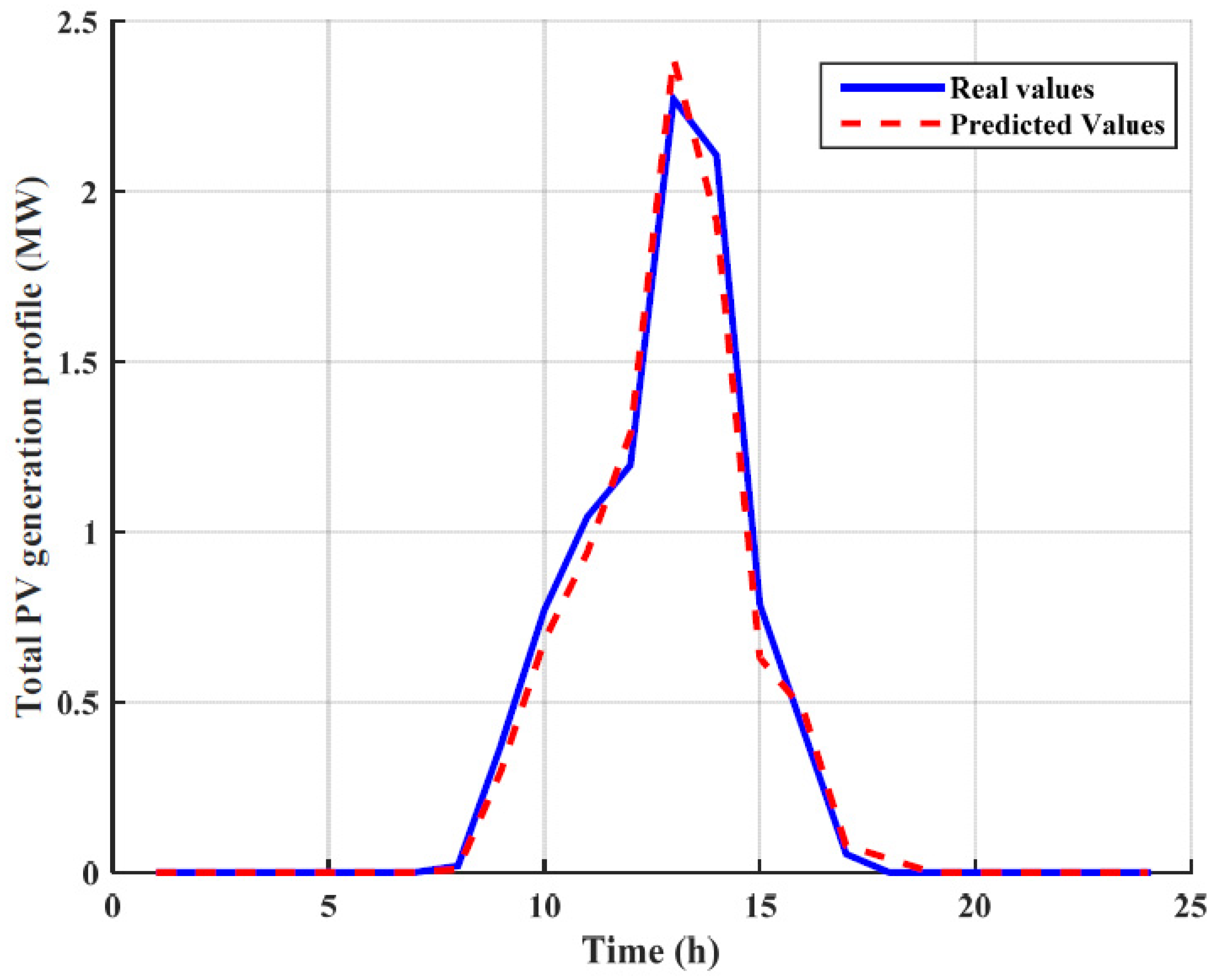
Figure 7, shows the real measured values of PV generation versus the predicted values obtained by ANNs available in MATLAB (R2014b, MathWorks, Natick, MA, USA). Analysis shows that the mean square error values and mean absolute percentage error are below 5%, which demonstrate the efficiency of the forecasting method.
Table 6 compares the simulation results in case of using the stochastic MPC and conventional stochastic method with different prediction errors. It can be realized that by implementing the stochastic MPC approach, robust results are reached with respect to the prediction errors. Moreover, the amount of total energy losses and total cost are decreased when an MPC-based approach is applied. In addition, the number of switching actions per day rises when the prediction error increases. Besides, utilizing the MPC approach results in better voltage regulation during the scheduling time horizon. As proposed in the last row of the Table 6, there is a limited difference among the execution times required by the solution of the proposed model with and without MPC approach.
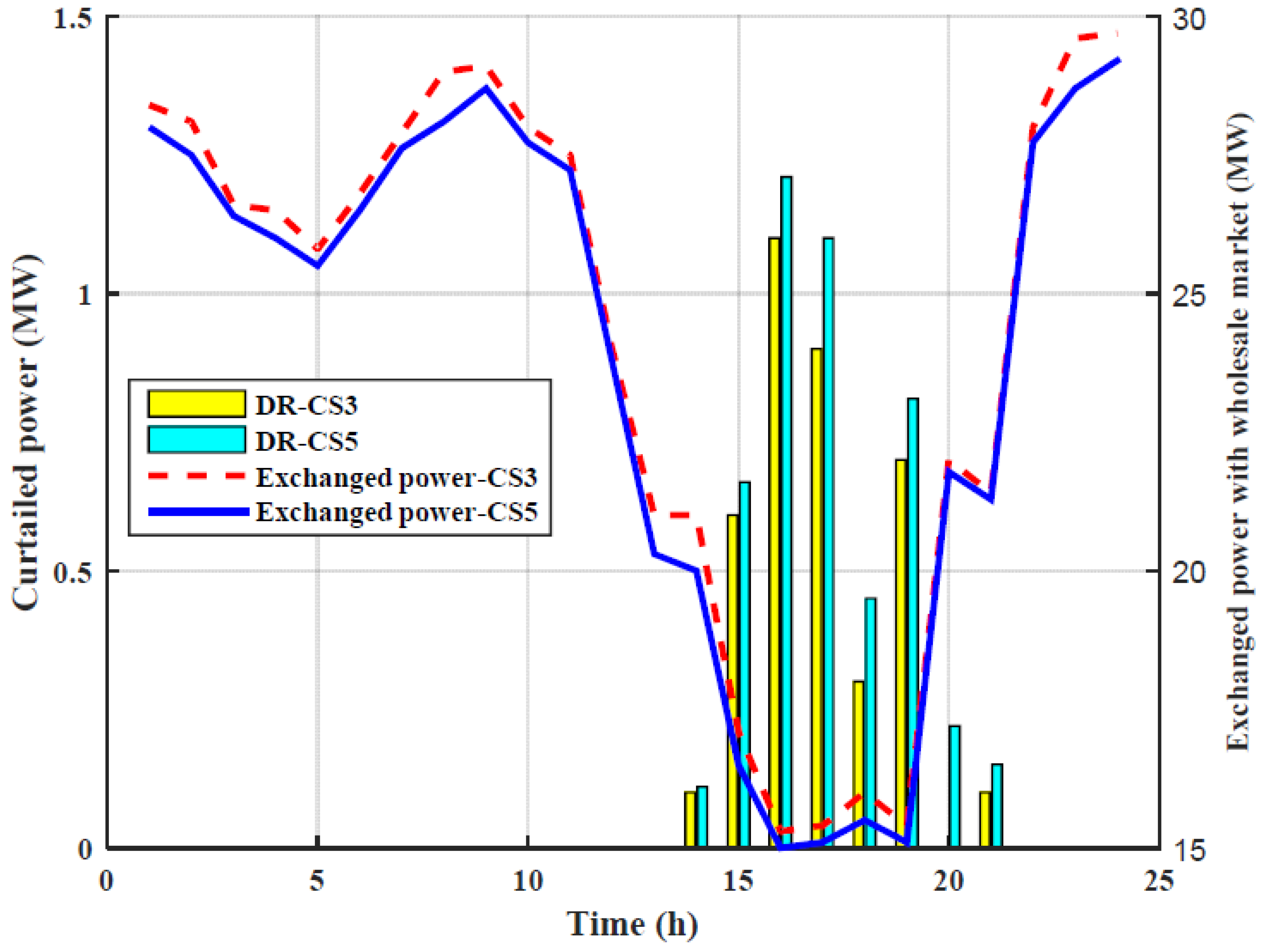
Figure 8 shows the amount of exchanged power with the wholesale market and the amount of curtailed power through participation of DRPs in CS3 and CS5. It can be seen that DSO purchases power from wholesale market during the 24-h time horizon. During the hours with higher electricity prices (i.e., 14:00–20:00), ESSs are discharged and MTs output power are increased. Thus, the amount of purchased power from wholesale market is decreased. Besides, the amount of purchased power is lower in CS5 than in CS3, which results in less total cost for CS5. Moreover, RLs are participated in DR programs through the bid-quantity packages during the hours with high market prices to flatten the power demand profile. It can be seen that hourly reconfiguration facilitates higher participation rates in DR programs. Table 7, summarizes the simulation results of different CSs for the proposed MILP-stochastic MPC model during the scheduling horizon. Results reveal the significant difference in the amount of energy loss, total cost, and the average voltage deviation among the aforementioned CSs. Compared to CS1, the total energy losses are decreased around 1% and 2% in CS2 and CS3, respectively, while the total costs are reduced by 1% and 3%, respectively. By implementing hourly reconfiguration in CS4 and CS5, the amount of energy losses is decreased by 6% and 11%, respectively, compared to CS1. Moreover, the results corresponding to CS4 and CS5 show that the total costs reduce 2135 $ and 4302 $, respectively. The latter reveals the substantial benefits of coordinating the ESSs, PVs, and RLs in a reconfigurable environment in the distribution systems. It can be seen that, in CS5 the integration of ESSs and DR programs through hourly reconfiguration, results to the best average voltage deviation amounts.
Figure 9, shows the average voltage profiles of each node for different CSs. By implementing the ESSs and DR programs in the model, the voltage profiles of the system are improved in CS2 and CS3. Moreover, the integration of ESSs and DR programs through hourly reconfiguration in CS5, leads to the best voltage profile. Active power loss of the system for different CSs over a day horizon is depicted in Figure 10. It can be deduced that implementation of the ESSs, DR programs, and hourly reconfiguration have a remarkable effect in decreasing the total power losses during the day, specifically 2%, 4%, 10%, and 12% reduction for CS2, CS3, CS4, and CS5, respectively compared to CS1.
The status of RCSs through the hourly reconfiguration process in CS5 is presented in Figure 11, where binary variables show the status of each RCS (1: closed status, 0: opened status). It can be seen that RCS no. 30 has the most number of switching actions among all the RCSs, i.e., six times in 24 h of scheduling, which is less than the calculated maximum number of switching actions for RCS 30 in Figure 5. Due to the calculated switching index in Figure 5, RCS1, RCS 2, RCS 3, RCS 18, RCS 19, and RCS 22 are not participated in the hourly reconfiguration, which are in line with the results of the Figure 11. Figure 12 investigates the performance of the proposed MPC approach regarding the different optimization time horizon steps. It can be concluded that by increasing the optimization time horizon steps, the amount of total cost is decreased and the execution time is increased. It can be seen that, by increasing a specific amount of steps, the execution time is increased significantly, while the amount of cost is decreased slightly. Hence, in this paper, 12-time steps, a trade-off between the execution time and the cost reduction, are considered as the optimization time horizon.

5. Conclusions

In this paper, a MILP-stochastic MPC model was proposed for operational scheduling of the distribution system from the DSO’s point of view to handle a dynamic and adaptive hourly reconfiguration. In order to survey the effect of implementing the ESSs, DRPs, and hourly reconfiguration on the total costs (including cost of total loss, switching cost, cost of bilateral contract with power generation owners and RL contributors, and cost of exchanging power with the wholesale market), different CSs were defined. Due to the uncertain nature of the problem, the stochastic MPC approach was applied in the optimization model. Moreover, a new index for switching actions based on the RCS ages and critical branch locations in the network along with the maximum number of switching was defined, which resulted in less allowable switching actions for aged or risky RCSs during the short-term scheduling. The performance of the proposed model was studied comprehensively on IEEE 33-bus distribution test system. It was shown that, by implementing the stochastic MPC approach, robust results are reached with respect to the prediction errors. It was concluded that by increasing the optimization time horizon steps, the execution time is increased and the amount of total cost is decreased. Hence, a trade-off between the execution time and the cost reduction was obtained. Moreover, the amount of total active power loss, total cost, and average bus voltage deviations could be decreased when the MPC-based approach is applied. Numerical results clearly showed the individual capability of ESSs and DR programs in decreasing the active power loss and total cost. More particular, coordinated integration of ESSs and DR programs through hourly reconfiguration decreases the total active power loss, total cost, and average bus voltage deviations during the scheduling horizon dramatically.

Author Contributions

S.E. designed the model. The input data was collected and analyzed by S.E. S.E. and A.A.-M. executed the simulation and accomplished the writing of the paper. S.J. and J.M.G. guided the whole work and edited language.

Funding

This research received no external funding.

Conflicts of Interest

The authors declare no conflict of interest.

Nomenclature

Indices and sets
tIndex of hour ( t = 1 , 2 , 3 , , T ).
i , j Index of buses ( i , j = 1 , 2 , , , N b u s ).
m Index of MTs ( m = 1 , 2 , 3 , , N M T ).
n Index of PVs ( n = 1 , 2 , 3 , , N P V ).
s Index of ESSs ( s = 1 , 2 , 3 , , N E S S ).
f Index of branches ( f = 1 , 2 , 3 , , N b r ).
q Index of DRPs ( q = 1 , 2 , 3 , , Q ).
ξ Index of steps in bid-quantity offers of DRPs ( ξ = 1 , 2 , 3 , , ϕ ).
k Index of RCSs ( k = 1 , 2 , 3 , , N s w ).
N ( i ) Set of buses connected to bus i
Parameters
g f , b f Conductance and suseptance of line f ( Ω ).
D Distance of each RCS from critical points.
N sub Number of substation buses.
H min q / H max q Minimum/maximum quantity of load reduction offered by qth DRP.
ρ ξ , t D R , q Offered price of DRP q for load reduction in step ξ at time t ($/MWh).
π s P V / π s W M / π s L Probability of scenarios related to PV output power/wholesale market price/demanded load.
N P V / N W M / N L Number of generated scenarios for PV output power/wholesale market price/demanded load.
η i c h / η i d c h Charging/Discharging efficiency of ESS i.
Variables
P t W M Exchanged power with the wholesale market at time t (MW).
P m , t M T Output power of MT m at time t (MW).
P t D R , q Day ahead scheduled load reduction quantity of DRP q at time t (MW).
V n o m Nominal voltage (kV).
B n , t P V Contracted price between PV owners and the DSO at time t ($/MWh).
B s , t E S S Contracted price between ESS owners and the DSO at time t ($/MWh).
B m , t M T Contracted price between MT owners and the DSO at time t ($/MWh).
ρ t W M Day-ahead wholesale market electricity price at time t ($/MWh).
ρ l o s s Cost of power losses ($/MWh).
ρ S W Cost of each switching action for RCSs ($).
A Age of RCSs.
N p , i j , t Number of path between bus i and bus j.
h ξ q Amount of accepted load reduction of DRP q in step ξ.
θ f Voltage angle difference of line f (radians).
V i Voltage magnitude at bus i (kV).
Δ V i , t Voltage deviations at bus i.
I i , j , t Current of line between bus i and bus j at time t (kA).
P t l o s s Power losses at time t (MW).
I i , j , t + / I i , j , t Auxiliary variable.
X i , j , t Status of line between bus i and bus j at time t.
N k , d a y S W Number of switching actions for RCS k per day.
S I k Switching index.
E i , t , s Energy storage of ESS i at time t (MWh).
P i , t f l o w / Q i , t f l o w Active/reactive power flow of bus i at time t (MW).
P s , t c h / P s , t d c h ESS i charge/discharge power at time t (MW).
P n , t P V Output power of PV n at time t (MW).
β i j Binary variables (1 if node i is the parent of node j).

References

  1. Xiang, Y.; Liu, J.; Liu, Y. Robust energy management of microgrid with uncertain renewable generation and load. IEEE Trans. Smart Grid 2016, 7, 1034–1043. [Google Scholar] [CrossRef]
  2. Konishi, R.; Takeda, A.; Takahashi, M. Optimal Sizing of Energy Storage Systems for the Energy Procurement Problem in Multi-Period Markets under Uncertainties. Energies 2018, 11, 158. [Google Scholar] [CrossRef]
  3. Aalami, H.A.; Nojavan, S. Energy storage system and demand response program effects on stochastic energy procurement of large consumers considering renewable generation. IET Gener. Trans. Distrib. 2016, 10, 107–114. [Google Scholar] [CrossRef]
  4. Fares, R.L.; Webber, M.E. A flexible model for economic operational management of grid battery energy storage. Energy 2014, 78, 768–776. [Google Scholar] [CrossRef]
  5. Marchi, B.; Zanoni, S.; Pasetti, M. A technoeconomic analysis of Li-ion battery energy storage systems in support of PV distributed generation. In XXI Summer School F. Turco of Industrial Systems Engineering; XXI Summer School “Francesco Turco”: Naples, Italy, 2016. [Google Scholar]
  6. Vahedipour-Dahraie, M.; Najafi, H.R.; Anvari-Moghaddam, A.; Guerrero, J.M. Security-constrained unit commitment in ac microgrids considering stochastic price-based demand response and renewable generation. Int. Trans. Electr. Energy Syst. 2018, e2596. [Google Scholar] [CrossRef]
  7. Nwulu, N.I.; Xia, X. Optimal dispatch for a microgrid incorporating renewables and demand response. Renew. Energy 2017, 101, 16–28. [Google Scholar] [CrossRef]
  8. Aghajani, G.R.; Shayanfar, H.A.; Shayeghi, H. Demand side management in a smart micro-grid in the presence of renewable generation and demand response. Energy 2017, 126, 622–637. [Google Scholar] [CrossRef]
  9. Pasetti, M.; Rinaldi, S.; Manerba, D. A Virtual Power Plant Architecture for the Demand-Side Management of Smart Prosumers. Appl. Sci. 2018, 8, 432. [Google Scholar] [CrossRef]
  10. Dantas, F.V.; Fitiwi, D.Z.; Santos, S.F.; Catalão, J.P. Dynamic reconfiguration of distribution network systems: A key flexibility option for RES integration. In Proceedings of the Environment and Electrical Engineering and 2017 IEEE Industrial and Commercial Power Systems Europe (EEEIC/I&CPS Europe), Milan, Italy, 6 June 2017; pp. 1–6. [Google Scholar]
  11. Asrari, A.; Lotfifard, S.; Payam, M.S. Pareto dominance-based multiobjective optimization method for distribution network reconfiguration. IEEE Trans. Smart Grid 2016, 7, 1401–1410. [Google Scholar] [CrossRef]
  12. Tahboub, A.M.; Pandi, V.R.; Zeineldin, H.H. Distribution system reconfiguration for annual energy loss reduction considering variable distributed generation profiles. IEEE Trans. Power Deliv. 2015, 30, 1677–1685. [Google Scholar] [CrossRef]
  13. Kaveh, M.R.; Hooshmand, R.A.; Madani, S.M. Simultaneous optimization of re-phasing, reconfiguration and DG placement in distribution networks using BF-SD algorithm. Appl. Soft Comput. 2018, 62, 1044–1055. [Google Scholar] [CrossRef]
  14. Ghofrani-Jahromi, Z.; Kazemi, M.; Ehsan, M. Distribution switches upgrade for loss reduction and reliability improvement. IEEE Trans. Power Deliv. 2015, 30, 684–692. [Google Scholar] [CrossRef]
  15. Gutiérrez-Alcaraz, G.; Galván, E.; González-Cabrera, N.; Javadi, M.S. Renewable energy resources short-term scheduling and dynamic network reconfiguration for sustainable energy consumption. Renew. Sustain. Energy Rev. 2015, 52, 256–264. [Google Scholar] [CrossRef]
  16. Nafisi, H.; Farahani, V.; Abyaneh, H.A.; Abedi, M. Optimal daily scheduling of reconfiguration based on minimisation of the cost of energy losses and switching operations in microgrids. IET Gener. Trans. Distrib. 2015, 9, 513–522. [Google Scholar] [CrossRef]
  17. Rokni, S.G.; Radmehr, M.; Zakariazadeh, A. Optimum energy resource scheduling in a microgrid using a distributed algorithm framework. Sustain. Cities Soc. 2018, 37, 222–231. [Google Scholar] [CrossRef]
  18. Bendato, I.; Bonfiglio, A.; Brignone, M.; Delfino, F.; Pampararo, F.; Procopio, R. A real-time Energy Management System for the integration of economical aspects and system operator requirements: Definition and validation. Renew. Energy 2017, 102, 406–416. [Google Scholar] [CrossRef]
  19. Anand, M.P.; Golshannavaz, S.; Ongsakul, W.; Rajapakse, A. Incorporating short-term topological variations in optimal energy management of MGs considering ancillary services by electric vehicles. Energy 2016, 112, 241–253. [Google Scholar] [CrossRef]
  20. Najibi, F.; Niknam, T. Stochastic scheduling of renewable micro-grids considering photovoltaic source uncertainties. Energy Convers. Manag. 2015, 98, 484–499. [Google Scholar] [CrossRef]
  21. Vahedipour-Dahraie, M.; Najafi, H.R.; Anvari-Moghaddam, A.; Guerrero, J.M. Optimal scheduling of distributed energy resources and responsive loads in islanded microgrids considering voltage and frequency security constraints. J. Renew. Sustain. Energy 2018, 10, 1–24. [Google Scholar] [CrossRef]
  22. Balasubramaniam, K.; Saraf, P.; Hadidi, R.; Makram, E.B. Energy management system for enhanced resiliency of microgrids during islanded operation. Electr. Power Syst. Res. 2016, 137, 133–141. [Google Scholar] [CrossRef]
  23. Vahedipour-Dahraie, M.; Anvari-Moghaddam, A.; Guerrero, J.M. Evaluation of reliability in risk-constrained scheduling of autonomous microgrids with demand response and renewable resources. IET Renew. Power Gener. 2018, 12, 657–667. [Google Scholar] [CrossRef] [Green Version]
  24. Parisio, A.; Rikos, E.; Glielmo, L. A model predictive control approach to microgrid operation optimization. IEEE Trans. Control Syst. Technol. 2014, 22, 1813–1827. [Google Scholar] [CrossRef]
  25. Verrilli, F.; Srinivasan, S.; Gambino, G.; Canelli, M.; Himanka, M.; Del Vecchio, C.; Sasso, M.; Glielmo, L. Model predictive control-based optimal operations of district heating system with thermal energy storage and flexible loads. IEEE Trans. Autom. Sci. Eng. 2017, 14, 547–557. [Google Scholar] [CrossRef]
  26. Parisio, A.; Rikos, E.; Glielmo, L. Stochastic model predictive control for economic/environmental operation management of microgrids: An experimental case study. J. Process Control 2016, 43, 24–37. [Google Scholar] [CrossRef] [Green Version]
  27. Zhang, Y.; Zhang, T.; Wang, R.; Liu, Y.; Guo, B. Optimal operation of a smart residential microgrid based on model predictive control by considering uncertainties and storage impacts. Sol. Energy 2015, 122, 1052–1065. [Google Scholar] [CrossRef]
  28. Safdarian, A.; Fotuhi-Firuzabad, M.; Lehtonen, M. Integration of price-based demand response in DisCos’ short-term decision model. IEEE Trans. Smart Grid 2014, 5, 2235–2245. [Google Scholar] [CrossRef]
  29. Vahedipour-Dahraie, M.; Rashidizaheh-Kermani, H.; Najafi, H.R.; Anvari-Moghaddam, A.; Guerrero, J.M. Coordination of EVs participation for load frequency control in isolated microgrids. Appl. Sci. 2017, 7, 539. [Google Scholar] [CrossRef]
  30. Esmaeili, S.; Vahidi, B.; Parvizimosaed, M.; Brahman, F. Development of a thermal and electrical energy management in residential building micro-grid. J. Renew. Sustain. Energy 2014, 6, 013126. [Google Scholar] [CrossRef]
  31. Santos, S.F.; Fitiwi, D.Z.; Shafie-Khah, M.; Bizuayehu, A.W.; Cabrita, C.M.; Catalão, J.P. New multistage and stochastic mathematical model for maximizing RES hosting capacity—Part I: Problem formulation. IEEE Trans. Sustain. Energy 2017, 8, 304–319. [Google Scholar] [CrossRef]
  32. Golshannavaz, S.; Afsharnia, S.; Aminifar, F. Smart distribution grid: Optimal day-ahead scheduling with reconfigurable topology. IEEE Trans. Smart Grid 2014, 5, 2402–2411. [Google Scholar] [CrossRef]
  33. Kavousi-Fard, A.; Khodaei, A. Efficient integration of plug-in electric vehicles via reconfigurable microgrids. Energy 2016, 111, 653–663. [Google Scholar] [CrossRef]
  34. Carpinelli, G.; Celli, G.; Mocci, S.; Mottola, F.; Pilo, F.; Proto, D. Optimal integration of distributed energy storage devices in smart grids. IEEE Trans. Smart Grid 2013, 4, 985–995. [Google Scholar] [CrossRef]
  35. Mazidi, M.; Monsef, H.; Siano, P. Robust day-ahead scheduling of smart distribution networks considering demand response programs. Appl. Energy 2016, 178, 929–942. [Google Scholar] [CrossRef]
  36. Dorostkar-Ghamsari, M.R.; Fotuhi-Firuzabad, M.; Lehtonen, M.; Safdarian, A.; Hoshyarzadeh, A.S. Stochastic Operation Framework for Distribution Networks Hosting High Wind Penetrations. IEEE Trans. Sustain. Energy 2017. [Google Scholar] [CrossRef]
  37. CPLEX Optimization Subroutine Library Guide and Reference; ILOG Inc.: Incline Village, NV, USA, 2008.
  38. Anand, A.; Suganthi, L. Hybrid GA-PSO Optimization of Artificial Neural Network for Forecasting Electricity Demand. Energies 2018, 11, 728. [Google Scholar] [CrossRef]
Figure 1. Conceptual design of the proposed Distribution Management System (DMS).
Energies 11 01884 g001
Figure 2. Procedure of the proposed stochastic Model Predictive Control (MPC).
Energies 11 01884 g002
Figure 3. A typical bid-quantity package for qth Demand Response Provider (DRP).
Energies 11 01884 g003
Figure 4. The IEEE 33-bus radial distribution test system.
Energies 11 01884 g004
Figure 5. (a) Switching index of each remotely controlled switch (RCS), (b) Daily maximum allowable switching actions.
Energies 11 01884 g005
Figure 6. Measured electrical load and real wholesale electricity market prices [32].
Energies 11 01884 g006
Figure 7. The real and predicted values for Photovoltaic (PV), generation profile over a day horizon.
Energies 11 01884 g007
Figure 8. Exchanged power with the wholesale market and the curtailed power through DRPs in CS3 and CS5.
Energies 11 01884 g008
Figure 9. Average nodal voltage deviations for different CSs over a day horizon.
Energies 11 01884 g009
Figure 10. Active power loss of the system for different CSs over a day horizon.
Energies 11 01884 g010
Figure 11. Status of RCSs through the hourly reconfiguration process in CS5.
Energies 11 01884 g011
Figure 12. Performance analysis of the MPC approach regarding different optimization time horizon steps.
Energies 11 01884 g012
Table 1. The details of bilateral contracts between Micro Turbine (MT) owners and Distribution System Operator (DSO).
Time Slot P m a x M T   ( MW ) P m i n M T   ( MW ) Price ($/MWh)
1:00–8:000438
9:00–16:0004110
17:00–24:000495
Table 2. Supported areas of Demand Response Providers (DRPs) in the distribution system.
DRPBuses
DRP13, 4, 5, 6, 7, 8, 19, 20, 21, 22
DRP210, 11, 12, 15, 16, 17, 30, 31, 32
Table 3. Bid quantity offer packages of DRPs.
DRPQuantity * (MW)
Price ** ($/MWh)
DRP10–0.3 *0.3–0.80.8–1.31.3–1.8
8.3 **18.123.952.5
DRP20–0.10.1–0.70.7–1.21.2–1.5
6.213.617.939.4
Table 4. Values for technical parameters.
ParameterValueParameterValue
V m i x , V m a x ( p . u . ) 0.95, 1.05 I i , j , m a x ( kA ) 0.8
η i c h , η i d c h ( p . u . ) 0.92, 0.92 P m a x W M ( MW ) 35
E min , E max   ( MWh ) 0.5, 2 E i i n i t i a l ( MWh ) 1
P min c h , P max c h ( MW ) 1 P min d c h , P max d c h ( MW ) 1
Table 5. Distinguishing the different Case Studies (CSs) (Energy Storage Systems (ESSs)).
CSESSsDRPsHourly Reconfiguration
CS1NoNoNo
CS2YesNoNo
CS3YesYesNo
CS4NoNoYes
CS5YesYesYes
Table 6. Evaluating the effectiveness of the proposed Mixed Integer Linear Programming (MILP)-stochastic MPC model in CS5.
Calculation resultsWithout MPCWith MPC
Prediction error (%)1020304010, 20, 30, 40
Energy loss (MWh)18.3118.4818.6319.0118.15
Total cost ($)53,42853,99254,21954,90751,807
Number of switching2832323428
Average bus voltage (p.u.)0.9820.9810.9810.9800.982
Execution time ** (s)7.717.837.928.019.95
** Programmed in GAMS using CPLEX solver in a computer with 2.6 GHz and 8 GB of RAM.
Table 7. Simulation results of different CSs for the proposed MILP-stochastic MPC model.
Calculation resultsCS1CS2CS3CS4CS5
Energy loss (MWh)20.3219.9119.5118.2918.15
Total cost ($)56,10955,82154,19053,97451,807
Number of switching actions---3228
Average voltage deviation (p.u.)0.9760.9770.9790.9800.982

