Forecasting Crude Oil Prices Using Ensemble Empirical Mode Decomposition and Sparse Bayesian Learning

Abstract

Crude oil is one of the most important types of energy and its prices have a great impact on the global economy. Therefore, forecasting crude oil prices accurately is an essential task for investors, governments, enterprises and even researchers. However, due to the extreme nonlinearity and nonstationarity of crude oil prices, it is a challenging task for the traditional methodologies of time series forecasting to handle it. To address this issue, in this paper, we propose a novel approach that incorporates ensemble empirical mode decomposition (EEMD), sparse Bayesian learning (SBL), and addition, namely EEMD-SBL-ADD, for forecasting crude oil prices, following the “decomposition and ensemble” framework that is widely used in time series analysis. Specifically, EEMD is first used to decompose the raw crude oil price data into components, including several intrinsic mode functions (IMFs) and one residue. Then, we apply SBL to build an individual forecasting model for each component. Finally, the individual forecasting results are aggregated as the final forecasting price by simple addition. To validate the performance of the proposed EEMD-SBL-ADD, we use the publicly-available West Texas Intermediate (WTI) and Brent crude oil spot prices as experimental data. The experimental results demonstrate that the EEMD-SBL-ADD outperforms some state-of-the-art forecasting methodologies in terms of several evaluation criteria such as the mean absolute percent error (MAPE), the root mean squared error (RMSE), the directional statistic (Dstat), the Diebold–Mariano (DM) test, the model confidence set (MCS) test and running time, indicating that the proposed EEMD-SBL-ADD is promising for forecasting crude oil prices.

1. Introduction

Crude oil is one of the dominant sources of energy that powers the global economy. The demand for crude oil will continue to increase, although its pace of growth is expected to slow gradually, according to the British Petroleum (BP) energy outlook 2017 [1]. Due to the importance of crude oil, many investors, governments, enterprises and even researchers pay much attention to the crude oil prices. However, a variety of factors such as speculation activities, supply and demand, technique development, geopolitical conflicts and wars can greatly produce effects on the prices of crude oil, making it show high nonlinearity and nonstationarity [2,3,4,5]. Therefore, it is a challenging task to forecast the crude oil prices accurately.

Various models have emerged to try to forecast the crude oil prices as accurately as possible in recent years. Generally speaking, the models can be roughly categorized into two groups: (1) statistical and econometric models; and (2) artificial intelligence (AI) models [5]. Typical models in the first group include vector autoregressive (VAR) models [6], the random walk model (RWM) [7,8], the autoregressive integrated moving average (ARIMA) [9,10] and generalized autoregressive conditional heteroskedasticity (GARCH) family models [11,12]. For example, Baumeister and Kilian demonstrated that VAR models could achieve good results when forecasting crude oil prices at short horizons [6]. Wang and Wu forecasted the volatility of crude oil prices using multivariate and univariate GARCH-class models, and the results indicated that the multivariate models showed better performance than univariate models [13]. Several ARIMA-GRARCHmodels for forecasting the volatility of crude oil prices were studied in 11 markets, and the forecasting results indicated that one of the models named APARCHoutperformed the others in most cases [14]. Some other research focused on a multivariate analysis of crude oil prices. Kruse and Wegener used model averaging to analyze time-varying persistence in real oil prices from more than one hundred and fifty variables and found that the index of global economic activity by Kilian [15] was the only significant measure to explain time-varying oil price persistence [16]. However, all the statistical and econometric models have the limitation that they are built on the assumption that the time series of crude oil prices has the characteristics of linearity and stationarity. Due to the high nonlinearity and nonstationarity, it is usually hard for these models to be directly applied to crude oil price forecasting to achieve satisfactory results. Therefore, the AI models have attracted increasing interest for crude oil price forecasting because they can capture the intrinsic features of nonlinearity and nonstationarity that exist widely in crude oil prices.

As for AI models, the most popular ones include the artificial neural network (ANN) and support vector regression (SVR). Mirmirani and Li used VAR and ANN with the genetic algorithm (GA) to forecast crude oil prices, and the results showed that ANN with GA significantly outperformed VAR [17]. The authors utilized ANN and fuzzy regression (FR) to forecast crude oil prices in the environment of noise, uncertainty and complexity, and the results indicated that the ANN was superior to FR regarding mean absolute percentage error (MAPE) [18]. The study suggested that the proposed ANN-GARCH approach was capable of improving the forecasting performance for both spot oil prices and future oil prices [19]. To further study the flexibility of ANN for forecasting crude oil prices, Jammazi and Aloui used the Haar a Trous Wavelet (HTW) decomposition and the multi-layer back propagation neural network (MBPNN) for decomposition and model building, respectively [20]. In the same research, the authors also analyzed the impacts of several activation functions and the levels of input-hidden nodes in ANN. The experimental results demonstrated that the proposed method performed better than the compared methods. Tang and Zhang built a multiple wavelet recurrent neural network model for crude oil price forecasting [21]. Different from some AI models that only consider the trend and the random components of crude oil prices, the model included gold prices in the forecasting. The experimental results indicated that the proposed model can achieve high forecasting accuracy.

From the perspective of machine learning, forecasting time series is a typical problem of regression that predicts the real value output based on the corresponding input. Therefore, in theory, any regression method in AI or the signal recovery method in signal processing can be applied to forecasting time series. In 2001, a novel method called sparse Bayesian learning (SBL) that used kernel-tricks was initially proposed as a machine learning method for both classification and regression [22]. Such SBL with kernel-tricks is also known as the relevance vector machine (RVM), a Bayesian competitor of the famous support vector machine (SVM). Later, it was found that SBL without kernel-tricks is a powerful tool for signal recovery, sparse representation and compressive sensing [23,24,25,26]. Therefore, SBL without kernel-tricks has the potential for forecasting crude oil prices.

Owing to the nonlinearity and nonstationarity, it is hard to forecast the movement of crude oil prices accurately using the raw price series directly. It has been reported that a novel “decomposition and ensemble” framework can significantly improve the forecasting accuracy for complex time series. In such a framework, the raw time series is first decomposed into several relatively simple components, then, each component is predicted by a single forecasting model, and finally, the results by each component are ensembled as the final results [27,28].

The commonly-used decomposition methods include wavelet decomposition (WD), independent component analysis (ICA), empirical mode decomposition (EMD), its variant ensemble empirical mode decomposition (EEMD), and so on, among which, EEMD is a popular one that has many advantages [5]. For the ensemble, much research has shown that the addition operation can achieve satisfactory results for time series forecasting. To further improve the forecasting efficiency and effectiveness, in this paper, we aim at proposing a novel method integrating EEMD, SBL and simple addition, namely, EEMD-SBL-ADD, to predict crude oil prices, following the “decomposition and ensemble” framework. Specifically, the raw series of crude oil prices is first decomposed into several components via EEMD. Then, SBL without kernel-tricks is applied to forecasting each component. Finally, the predicted values of each component are added as the final results. The main contributions of this paper are as follows: (1) A novel forecasting approach for crude oil prices that combines EEMD, SBL and addition was proposed, following the well-known “decomposition and ensemble” framework. To the best of our knowledge, this is the first time that SBL without kernel-tricks has been applied to forecasting time series. (2) Extensive experiments were conducted on the publicly-accessible West Texas Intermediate (WTI) and Brent spot crude oil prices, and it was shown that the proposed approach outperformed several state-of-the-art methods for forecasting crude oil prices. (3) We further analyzed the characteristics of SBL when applied to forecasting crude oil prices, such as running time, the impact of the lag order and SBL’s parameter settings (scalar trade-off parameter and iteration number) on the forecasting performance.

It is worth pointing out that the proposed EEMD-SBL-ADD is different from some previous work on forecasting crude oil prices [5], wind power [29] and electricity price [30], where kernel-tricks are adopted in the SBL framework. The proposed EEMD-SBL-ADD utilized SBL without kernel-tricks to forecast each component decomposed from raw crude oil prices.

The rest of this paper is organized as follows. Section 2 briefly gives the description of EEMD and SBL. Section 3 formulates the proposed EEMD-SBL-ADD method in detail. For the purpose of evaluating the proposed method, experimental results are reported and discussed in Section 4. Finally, Section 5 concludes this paper.

2. Preliminaries

2.1. Ensemble Empirical Mode Decomposition

EEMD is proposed on the basis of empirical mode decomposition (EMD) [31,32]. The latter is a kind of adaptive signal decomposition method after Fourier spectral analysis and wavelet analysis. It has been widely studied and applied to nonlinear and nonstationary signal or time series. However, it was reported that the IMF components decomposed by EMD often result in the “mode mixing” problem [33]. That is to say, the same IMF component contains a time series with wide scale and different ranges or different IMF components contain time series with similar scales. The consequence of “mode mixing” is that the IMF component no longer has the same characteristic timescale and becomes a scale-dependent oscillation, thereby losing the original physical meaning. To represent the signal better, EEMD was proposed to reduce “mode mixing” and extract the real model effectively [32]. Its main idea is to eliminate “mode mixing” by the characteristics of the uniform energy distribution and whole average meaning. Several white noises are added into the original time series. Then, the EMD processing is performed many times individually. Finally, the average value is obtained for the real mode. The steps of EEMD are as follows:

Step 1: Specify the standard Gaussian white noises $\sigma$, the ensemble number I and a loop variable $i=1$;

Step 2: Add a Gaussian white noise $n_i\left(t\right)\sim N(0,{\sigma }^2)$ to the raw crude oil price series $X\left(t\right)$ to obtain the following new series as Equation (1):

$$X_i\left(t\right)=X\left(t\right)+n_i\left(t\right),$$

(1)

Step 3: Perform EMD on $X_i\left(t\right)$ to obtain m IMFs $c_{ij}\left(t\right)(j=1,2,\cdots ,m)$ and one residue $r_i\left(t\right)$ as Equation (2):

$$X_i\left(t\right)=\sum _{j=1}^m{c}_{ij}\left(t\right)+r_i\left(t\right),$$

(2)

where $c_{ij}$ represents the $j-$IMF for the i-th trail and m is the number of IMFs, determined by the length of crude oil price series T with $m=\lfloor lo{g}_{2}T\rfloor -1$ [32].

Step 4: $i=i+1$, if $i>M$, go to Step 5; otherwise, go to Step 2;

Step 5: Compute the j-th final IMF $C_j\left(t\right)$ with corresponding IMFs in I trials as Equation (3):

$$C_j\left(t\right)=\frac{1}{I}\sum _{i=1}^I{c}_{ij}\left(t\right),j=1,2,\cdots ,m.$$

(3)

Step 6: Compute the final residue $r\left(t\right)$ as Equation (4):

$$r\left(t\right)=X\left(t\right)-\sum _{j=1}^m{C}_j\left(t\right).$$

(4)

It can be seen that with EEMD, the raw crude oil price series $X\left(t\right)$ can be expressed as the sum of m IMFs $C_j\left(t\right)(j=1,2,\cdots ,m$) and one residue $r\left(t\right)$. The forms of the IMFs and the residue are usually simpler than that of the raw crude oil price series. Now, the hard work of forecasting the complex, nonlinear and nonstationary raw price data is divided into forecasting several relatively simple components (m IMFs and one residue).

2.2. Sparse Bayesian Learning

Sparse Bayesian learning (SBL) was first proposed as a machine learning method that uses kernel-tricks [34] Tipping2001, and it has shown its power in various practical classification and regression applications, such as image classification [34], object detection [35], oil production prediction [36], automatic seizure detection [37], deception detecting [38], fault diagnosis [39], and so on. However, later, SBL without kernel-tricks has also been demonstrated to be effective and efficient on sparse signal recovery, sparse representation and compressive sensing [23,26,40]. In many ways, signal recovery can be thought of as regression because their goals are to minimize the generalization error. Therefore, in this paper, we use SBL without the kernel-trick to forecast crude oil prices. For the convenience of expression, in the rest of this paper, SBL refers to sparse Bayesian learning without kernel-tricks, unless otherwise stated.

Sparse signal recovery can be formulated by Equation (5):

$$y=\Phi w+ϵ,$$

(5)

where $\Phi \in R^{N\times M}$ is a matrix with N samples and each sample has M features, $y={[y_1,y_2,\cdots ,y_N]}^T$ is a vector of targets, $ϵ$ is noise and $w={[w_1,w_2,\cdots ,w_M]}^T$ is the vector to be learned to represent the weights of each column in $\Phi$. The objective of SBL is to seek a vector of weights w that has many entities of zeros, while it can still approximate the targets y accurately [23].

In the SBL framework, it assumes the Gaussian likelihood model as Equation (6):

$$p\left(y\right|w;{\sigma }^2)={\left(2\pi {\sigma }^2\right)}^{-\frac{N}{2}}exp(-\frac{1}{2{\sigma }^2}\left|\right|y-{\Phi w\left|\right|}^2).$$

(6)

Under such conditions, the task of obtaining maximum likelihood estimates for w equals the task of finding the minimum ${\ell }_2$-norm solution to Equation (5). However, such solutions are usually non-sparse. To find sparse solutions, SBL estimates a parameterized prior over weights from the data by Equation (7):

$$p(w;\gamma )=\prod _{i=1}^M{\left(2\pi {\gamma }_i\right)}^{-\frac{1}{2}}exp(-\frac{w_i^2}{2{\gamma }_i}),$$

(7)

where $\gamma ={[{\gamma }_1,{\gamma }_2,\cdots ,{\gamma }_M]}^T$ is a vector of M hyperparameters that controls the prior variance of each weight. The procedure of estimating these hyperparameters from data consists of two steps: (1) marginalizing over the weights and (2) performing the maximum likelihood optimization algorithm. Interested readers can refer to [23] for more details.

The advantages of SBL are as follows:

• Unlike many other sparse learning algorithms that require $M\gg N$ in the matrix $\Phi$ in Equation (5), SBL can still achieve satisfactory results even when $M<N$.
• There are few parameters to set in SBL, and hence, it is not necessary to optimize parameters so that the training procedure is very fast and the results are more robust.
• The weights found by SBL can measure the importance of each feature on forecasting crude oil prices, which improves the ability of interpretability of each feature.
• Since SBL is suitable for resolving the multiple measurement vector model, it is easy to handle forecasting crude oil prices at several horizons simultaneously.

3. The Proposed EEMD-SBL-ADD Approach

Inspired by the power of EEMD on signal preprocessing and the advantages of SBL on signal recovery or regression, this paper proposes a novel approach that integrates EEMD, SBL and addition, termed EEMD-SBL-ADD, for forecasting crude oil prices, following the “decomposition and ensemble” framework. The approach is shown in Figure 1, which consists of three stages:

Stage 1:

Decomposition. EEMD is applied to decompose the raw series of crude oil prices $X\left(t\right)(t=1,2,\cdots ,T)$ into two parts: (1) $m=\lfloor lo{g}_{2}T\rfloor$ IMF components $C_j\left(t\right)(j=1,2,\cdots ,m)$; (2) one residue component $r\left(t\right)$.

Stage 2:

Individual forecasting. For each component from Stage 1, the data samples in the component are divided into a training set and a test set. The SBL predictor is built on the training set, and then, the predictor is applied to the test set.

Stage 3:

Ensemble forecasting. The test results of all components from Stage 2 are aggregated by simple addition as the final forecasting results.

The proposed EEMD-SBL-ADD is a typical strategy of “divide and conquer”, where the complicated issue of forecasting the original crude oil prices is transformed to several relatively simple issues of forecasting components independently. The EEMD-SBL-ADD first uses EEMD to decompose the original crude oil price series into several components, and each component reflects some characteristics of crude oil prices. For example, the first several IMFs reflect high-frequency parts, while the last several IMFs and the residue reflect the low-frequency parts of the crude oil prices. Secondly, the EEMD-SBL-ADD builds a forecasting model for each single component using SBL, and then, the forecasting model can predict the test data of each single component. Finally, the predicted values from each component can be aggregated as the final forecasting results of crude oil prices. All these characteristics make it possible for the EEMD-SBL-ADD to improve the performance for forecasting crude oil prices.

4. Experimental Results

4.1. Data Description

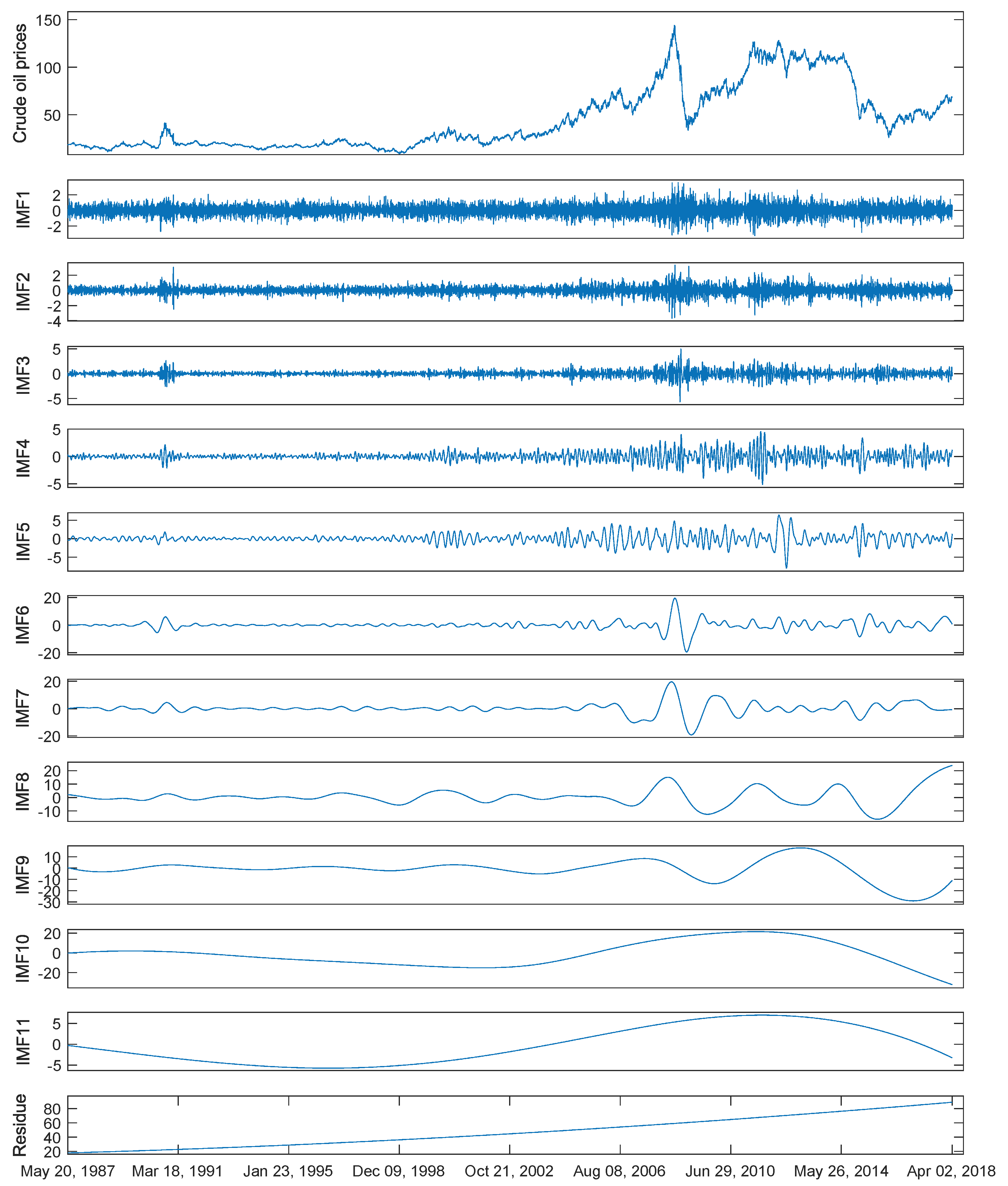
To validate the performance of the proposed EEMD-SBL-ADD, this paper used two publicly-accessed crude oil price series, i.e., West Texas Intermediate (WTI) crude oil spot prices and Brent crude oil spot prices, for their representative significance in international crude oil markets. For WTI data series, we used the daily close prices from 2 January 1986–2 April 2018, with a total 8132 samples, as experimental data. Among the samples, the first 6506 ones accounting for 80% from 2 January 1986–13 October 2011 were used as training samples, and the remaining 1626 ones accounting for 20% from 14 October 2011–2 April 2018 were used as testing samples. Meanwhile, for Brent data series, 7836 samples of daily close prices from 20 May 1987–2 April 2018 were used. The dataset was also split as done for the WTI dataset: the first 80% of samples for training and the remaining 20% for testing. The original crude oil prices and corresponding components decomposed by EEMD of WTI and Brent are shown in Figure 2 and Figure 3, respectively.

4.2. Evaluation Criteria

In order to evaluate the model from multiple views, we selected four evaluation indexes: the mean absolute percent error (MAPE), the root mean squared error (RMSE), the directional statistic ($D_{stat}$) and the Diebold–Mariano (DM) statistic. At first, we used RMSE and MAPE to evaluate the prediction accuracy. MAPE and RMSE are defined as Equations (8) and (9), respectively:

$$\mathrm{MAPE}=\frac{1}{n}\sum _{t=1}^n\left|\frac{y_t-{\widehat{y}}_t}{y_t}\right|,$$

(8)

$$\mathrm{RMSE}=\frac{1}{n}\sqrt{\sum _{t=1}^n{(y_t-{\widehat{y}}_t)}^2},$$

(9)

where $y_t$ is the actual value, ${\widehat{y}}_t$ is the predicted value at time t and n is the total number of test sets.

Then, we selected the directional statistic ($D_{stat}$) to evaluate the ability of direction prediction. $D_{stat}$ is defined as Equation (10):

$$D_{stat}=\frac{1}{n}\sum _{t=1}^n{a}_t\times 100\%,$$

(10)

where $a_t=\left\{\begin{array}{c}1, (y_t-y_{t-1})({\widehat{y}}_t-y_{t-1})\ge 0;\hfill \\ 0, \mathrm{otherwise}.\hfill \end{array}\right.$.

Obviously, the lower the MAPE and RMSE values, the higher the prediction accuracy is. In contrast, the higher the $D_{stat}$ value, the more accurate the direction prediction of the model is.

Next, we utilized the Diebold–Mariano (DM) statistic to compare the prediction errors of two models, which is defined as Equation (11):

$$S=\frac{\overline{d}}{\sqrt{Var\left(\overline{d}\right)}},$$

(11)

where $\overline{d}=\frac{1}{n}{\displaystyle \sum _{t=1}^n}{d}_t$, $d_t={(y_t-{\widehat{y}}_{1t})}^2-{(y_t-{\widehat{y}}_{2t})}^2$, $Var(\overline{d})=\frac{1}{n}({\gamma }_0+2{\displaystyle \sum _{k=1}^{n-1}}{\gamma }_k)$ and ${\gamma }_k=\mathrm{cov}(d_t,d_{t-k})$. ${\widehat{y}}_{1t}$ represents the predicted values obtained by the first model at time t, while ${\widehat{y}}_{2t}$ is obtained by the second model. The original assumption of this statistic is that the two models have equal prediction accuracy. When the statistic is negative, the first model is statistically advantageous compared to the second one.

Finally, since the multiple application of the DM test for a set of pairwise comparisons provides biased p-values, the model confidence set (MCS) was applied to further demonstrate SBL’s superiority to other models on crude oil price forecasting. The MCS can be used to select the optimal model from several models for prediction, and the results are robust [41].

To obtain more data to calculate the p-value of the statistics, the MCS performs a bootstrap on the prediction sequence. For the j-th models, given the size of bootstrapped sample T, the t-th bootstrapped sample has the loss defined as Equation (12):

$$L_{j,t}=\frac{1}{T}\sum _{i=h+1}^{h+T}|y_i-{\widehat{y}}_i|.$$

(12)

Given a set $M_0=\{m_i,i=1,2,\cdots ,n\}$ that contains n models, for any two models j and k, the relative values of the loss between these two models can be defined as Equation (13):

$$d_{j,k,t}=L_{j,t}-L_{k,t}.$$

(13)

With the above definitions, the set of superior models can be defined as Equation (14):

$$M^{*}\equiv m_j\in M_0:E\left(d_{j,k,t}\right)\le 0, \forall m_k\in M_0.$$

(14)

where $E(.)$ represents the average value.

The MCS performs a series of significant tests in $M_0$. Each time, the worst prediction model in the set is eliminated. In each test, the hypothesis is the null hypothesis of equal predictive ability (EPA), defined as Equation (15):

$$H_0:E\left(d_{j,k,t}\right)=0, \forall m_j,m_k\in M\subset M_0.$$

(15)

The MCS mainly relies on the equivalence test and elimination criteria. The specific process is as follows:

Step 1:

Assuming $M=M_0$, at the level of significance $\alpha$, use the equivalence test to test the null hypothesis $H_{0,M}$;

Step 2:

If it accepts the null hypothesis, then $M_{1-\alpha }^{*}=M$ will be defined; otherwise, the model that rejects the null hypothesis from M will be eliminated by the elimination criteria. The elimination will not stop until there are no longer any models rejecting the null hypothesis in the set M. At last, the models in the $M_{1-\alpha }^{*}$ are thought as surviving models.

The MCS has two kinds of statistics that can be defined as Equations (16)–(18).

$$T_R=\underset{j,k\in M}{max}\frac{|\overline{d_{j,k}}|}{\sqrt{var\left(\overline{d_{j,k}}\right)}},$$

(16)

$$T_{SQ}=\underset{j,k\in M}{max}\frac{{\left(\overline{d_{j,k}}\right)}^2}{var\left(\overline{d_{j,k}}\right)},$$

(17)

$$\overline{d_{j,k}}=\frac{1}{T}\sum _{t=h+1}^{h+T}{d}_{j,k,t}.$$

(18)

The p-value can be computed with these statistics, and then, it can be used to determine the elimination or survival of the models. When the p-value of one model is less than the significance level $\alpha$, this model will be eliminated; otherwise, it will survive. The larger the p-value, the more accurate the prediction of the model. When the p-value is equal to one, it indicates that the model is the optimal forecasting model.

4.3. Experimental Settings

To demonstrate the power of SBL on crude oil price forecasting, we firstly conducted experiments on raw series, and this is the so-called single model. We compared SBL with three very popular models of time series forecasting, i.e., one statistical model, ARIMA, and two AI models, ANN and LSSVR. Then, we ran ensemble models on the decomposed signals. To set up the stage for a fair comparison, we used addition (ADD) to aggregate the individual forecasting result of each component as the final result. We compared the proposed EEMD-SBL-ADD with the other seven ensemble models (EEMD-ARIMA-ADD, EEMD-ANN-ADD, EEMD-LSSVR-ADD, EMD-SBL-ADD, EMD-ARIMA-ADD, EMD-ANN-ADD and EMD-LSSVR-ADD) to further validate the performance of the proposed approach. Among the ensemble models, the ones with SBL, ANN or LSSVR are called AI-based ensemble models in this paper.

For SBL, we set 0.0004 and 600 as the values of the scalar trade-off parameter for balancing sparsity and data fit and the maximum number of iterations, respectively. For ARIMA, we needed to determine the values of the three parameters ($p-d-q$). d represents the number of times a nonstationary sequence turns into a stationary sequence. p and q represent the autocorrelation coefficient and partial correlation coefficient, respectively. We selected the optimal values of p and q through the AIC (Akaike information criterion) rule. For the parameters of ANN, we selected the BP (back propagation) neural network and used a four-layer network with two hidden layers. The number of hidden layer nodes was set to seven, and the maximum number of training steps was set to 10,000. For LSSVR, we chose the very popular RBF as the kernel of the model. Then, we needed to select two important parameters, including the regularization parameter $\gamma$ and kernel parameter ${\sigma }^2$. We used grid search to find the optimal values for both parameters, following [28,42].

Data normalization is an important work for AI-based time series forecasting. On the one hand, normalization can accelerate finding the optimal solution for gradient descent; on the other hand, it allows the characteristics of different dimensions to be comparable in numerical terms and may improve accuracy. To set up a fair comparison, in the paper, we used a frequently-used normalization method (the Min-Max normalization) for AI-based predictors. Note that ARIMA does not need normalization. The normalization formula is as Equation (19):

$$y_{norm}=\frac{y-y_{min}}{y_{max}-y_{min}},$$

(19)

where $y_{max}$ and $y_{min}$ are the maximum and minimum values of the original dataset, respectively. y and $y_{norm}$ are the raw values and the normalized values. The normalization maps the raw values in the range of [0,1].

Finally, we needed to do the inverse normalization after we obtained the predicted values by normalization. The formula is as Equation (20):

$$\widehat{y}={\widehat{y}}_{norm}\times (y_{max}-y_{min})+y_{min},$$

(20)

where ${\widehat{y}}_{norm}$ is the predicted value before inverse normalization and $\widehat{y}$ is the final predicted value we need.

In addition, we performed multi-step-ahead prediction and selected horizons of 1, 2, 3, 4, 5 and 6 as experimental objects. If we want to predict the value of $y_{t+h}$ with a time series $y_t$, ($t=1,2,3,\cdots ,T$), it can be formulated as Equation (21):

$${\widehat{y}}_{t+h}=f(y_t,y_{t-1},y_{t-2},\cdots ,y_{t-(l-1)}),$$

(21)

where ${\widehat{y}}_{t+h}$ represents the predicted value of $y_{t+h}$, $y_t$ represents the actual value at time tand l is the lag order. As suggested by [43], we set six as the lag order in these experiments. For the MCS, we set 0.2 as the level of significance $\alpha$ and 5000 as the number of bootstrapped samples. Meanwhile, we used “stationary” as the boot type.

All the experiments were conducted by MATLAB R2016b on a 64-bit Windows 10 professional edition with an i7-7820X CPU @3.6 GHz and 32 GB RAM.

4.4. Results and Analysis

4.4.1. Single Models

The MAPE values for single models on WTI and Brent crude oil prices are shown in

Table 1. The MAPE values by different single models on WTI and Brent crude oil prices.

	Model	SBL	ARIMA	ANN	LSSVR
Horizon
WTI	One	0.0154	0.0152	0.0151	0.0204
	Two	0.0206	0.0210	0.0210	0.0210
	Three	0.0255	0.0260	0.0261	0.0257
	Four	0.0295	0.0303	0.0302	0.0297
	Five	0.0329	0.0340	0.0332	0.0334
	Six	0.0364	0.0379	0.0370	0.0367
Brent	One	0.0134	0.0136	0.0135	0.0144
	Two	0.0198	0.0201	0.0200	0.0205
	Three	0.0250	0.0255	0.0251	0.0255
	Four	0.0291	0.0299	0.0293	0.0296
	Five	0.0328	0.0337	0.0334	0.0333
	Six	0.0360	0.0372	0.0373	0.0366

. Among the models, SBL achieved the lowest (the best) values in 11 out of 12 cases on both markets, while ARIMA, ANN and LSSVR achieved the highest (the worst) values in 7/12, 3/12 and 4/12 cases (note that some models achieved the same highest values at some horizons). The results achieved by the statistical model ARIMA were slightly higher than, but very close to those by ANN or LSSVR in most cases. For each model, with the increase of the horizon, the corresponding MAPE values were increasing.

As another level performance of forecasting, the RMSE values of all the models at different horizons on WTI and Brent crude oil prices are shown in

Table 2. The RMSE values by different single models on WTI and Brent crude oil prices.

	Model	SBL	ARIMA	ANN	LSSVR
Horizon
WTI	One	1.2622	1.2770	1.2757	1.2925
	Two	1.7153	1.7454	1.7387	1.7430
	Three	2.0943	2.1415	2.1282	2.1097
	Four	2.4041	2.4731	2.4303	2.4146
	Five	2.6781	2.7717	2.6823	2.6917
	Six	2.9327	3.0548	2.9714	2.9489
Brent	One	1.1961	1.2097	1.1974	1.2659
	Two	1.7366	1.7669	1.7377	1.7885
	Three	2.1525	2.2042	2.1677	2.1929
	Four	2.4895	2.5643	2.4954	2.5246
	Five	2.7817	2.8837	2.8257	2.8179
	Six	3.0521	3.1866	3.1539	3.0941

. It can be seen that SBL outperformed all other models in all cases, while ARIMA obtained the worst values in 9 out of 12 cases, showing that the ARIMA had poor power for forecasting raw crude oil prices. For ANN and LSSVR, they achieved very close results, and neither of them was always superior to the other one.

For the directional prediction, it can be seen from

Table 3. The Dstat values by different single models on WTI and Brent crude oil prices.

	Model	SBL	ARIMA	ANN	LSSVR
Horizon
WTI	One	0.4926	0.4803	0.4945	0.5251
	Two	0.5178	0.5068	0.5117	0.5172
	Three	0.4883	0.4963	0.5006	0.4988
	Four	0.4926	0.5000	0.5074	0.5018
	Five	0.4945	0.4889	0.4988	0.4994
	Six	0.4994	0.4859	0.4902	0.4920
Brent	One	0.5086	0.5182	0.5341	0.5067
	Two	0.5061	0.5010	0.5003	0.4978
	Three	0.4965	0.4933	0.4952	0.5080
	Four	0.4914	0.4990	0.4990	0.4978
	Five	0.4876	0.5016	0.4837	0.4888
	Six	0.5041	0.4933	0.4959	0.4971

that none of the models can always outperform any other ones. Amongst the models, SBL, ARIMA, ANN and LSSVR obtained the highest values on 4/12, 2/12, 4/12 and 3/12 cases, respectively (ARIMA and ANN achieved the highest values simultaneously at Horizon 4 on Brent crude oil prices). The results also demonstrated that the performance of single models was not stable when forecasting the direction of crude oil prices. Another interesting finding was that the highest value in all cases was 0.5341, while the lowest value was 0.4803, which were very similar to the result of a random guess. Therefore, it was hard for single models to achieve a satisfactory directional prediction, and the hidden reason was probably the nonlinearity and nonstationarity of the complex crude oil prices.

This paper also used the DM test to validate the superiority of the SBL from the viewpoint of statistics, as the statistics and p-values (in brackets) shown in

Table 4. The Diebold–Mariano (DM) test results for single models on WTI crude oil prices.

Benchmark	One-Step-Ahead			Two-Step-Ahead			Three-Step-Ahead
Tested model	ARIMA	ANN	LSSVR	ARIMA	ANN	LSSVR	ARIMA	ANN	LSSVR
SBL	−3.05	−3.25	−3.13	−2.53	−3.04	−2.87	−2.22	−2.90	−1.53
	(0.0023)	(0.0012)	(0.0018)	(0.0116)	(0.0024)	(0.0042)	(0.0266)	(0.0038)	(0.1252)
ARIMA	0.31	−1.33		0.55	0.13		0.60	1.17
		(0.7573)	(0.1839)		(0.5795)	(0.8952)		(0.5494)	(0.2424)
ANN			−1.42			−0.36			1.21
			(0.1558)			(0.7199)			(0.2279)
Benchmark	Four-Step-Ahead			Five-Step-Ahead			Six-Step-Ahead
Tested model	ARIMA	ANN	LSSVR	ARIMA	ANN	LSSVR	ARIMA	ANN	LSSVR
SBL	−2.09	−1.46	−0.95	−1.99	−0.19	−1.08	−1.97	−1.71	−1.00
	(0.0365)	(0.1435)	(0.3432)	(0.0473)	(0.8508)	(0.2811)	(0.0492)	(0.0878)	(0.3186)
ARIMA		1.20	1.48		2.06	1.48		1.29	1.50
		(0.2316)	(0.1387)		(0.0397)	(0.1398)		(0.1662)	(0.1331)
ANN			0.74			−0.40			0.90
			(0.4619)			(0.6924)			(0.3704)

and

Table 5. The DM test results for single models on Brent crude oil prices.

Benchmark	One-Step-Ahead			Two-Step-Ahead			Three-Step-Ahead
Tested model	ARIMA	ANN	LSSVR	ARIMA	ANN	LSSVR	ARIMA	ANN	LSSVR
SBL	−2.04	−0.28	−7.04	−1.73	−0.17	−4.06	−1.66	−1.31	−2.77
	(0.0412)	(0.7778)	(0.0000)	(0.0839)	(0.8658)	(0.0001)	(0.0969)	(0.1907)	(0.0057)
ARIMA		1.54	−4.31		1.74	−0.91		0.95	0.3096
		(0.1235)	(0.0000)		(0.0819)	(0.3651)		(0.3425)	(0.7569)
ANN			−6.11			−3.33			−1.82
			(0.0000)			(0.0009)			(0.0692)
Benchmark	Four-Step-Ahead			Five-Step-Ahead			Six-Step-Ahead
Tested model	ARIMA	ANN	LSSVR	ARIMA	ANN	LSSVR	ARIMA	ANN	LSSVR
SBL	−1.56	−0.46	−1.91	3.52	−1.33	−1.56	−1.47	−1.75	−1.49
	(0.1188)	(0.6433)	(0.0558)	(0.0004)	(0.1849)	(0.1186)	(0.1423)	(0.0811)	(0.1355)
ARIMA		1.36	0.74		−3.41	−3.43		0.29	0.94
		(0.1744)	(0.4577)		(0.0007)	(0.0006)		(0.7885)	(0.3451)
ANN			−1.86			0.25			1.04
			(0.0631)			(0.8002)			(0.2970)

. The results further statistically confirmed the above conclusions. First, the SBL statistically outperformed ARIMA, ANN, and LSSVR, and the corresponding p-values were far below 0.1 in 21 out of 36 cases. Second, when we chose the statistical model ARIMA as the benchmark model; ARIMA was statistically shown to underperform compared to the the AI models, showing that the latter were more powerful for forecasting nonlinear and nonstationary crude oil prices. Finally, regarding ANN and LSSVR, the results showed that neither of them could significantly outperform the other one.

We further report the results of the MCS test by single models on both WTI and Brent crude oil prices, as shown in

Table 6. The model confidence set (MCS) test results by different single models on WTI and Brent crude oil prices.

Model		Horizon
		One		Two		Three		Four		Five		Six
		${\mathit{T}}_{\mathit{R}}$	${\mathit{T}}_{\mathit{SQ}}$	${\mathbf{T}}_{\mathbf{R}}$	${\mathit{T}}_{\mathit{SQ}}$	${\mathit{T}}_{\mathit{R}}$	${\mathit{T}}_{\mathit{SQ}}$	${\mathit{T}}_{\mathit{R}}$	${\mathit{T}}_{\mathit{SQ}}$	${\mathit{T}}_{\mathit{R}}$	${\mathit{T}}_{\mathit{SQ}}$	${\mathit{T}}_{\mathit{R}}$	${\mathit{T}}_{\mathit{SQ}}$
WTI	LSSVR	0.0006	0.0016	0.0114	0.0114	0.0970	0.0970	0.5604	0.5604	0.3048	0.3048	0.1390	0.1390
	ANN	0.0006	0.0004	0.0034	0.0020	0.0118	0.0028	0.0254	0.0058	0.0258	0.0202	0.0112	0.0134
	ARIMA	0.0006	0.0016	0.0034	0.0040	0.0118	0.0128	0.0254	0.0322	0.0258	0.0206	0.0112	0.0134
	SBL	1.0000	1.0000	1.0000	1.0000	1.0000	1.0000	1.0000	1.0000	1.0000	1.0000	1.0000	1.0000
Brent	LSSVR	0.0000	0.0000	0.0004	0.0018	0.0394	0.0322	0.2228	0.1744	0.1050	0.0964	0.0584	0.0584
	ANN	0.5880	0.5880	0.4988	0.4988	0.5806	0.5806	0.7512	0.7512	0.1050	0.0964	0.0488	0.0268
	ARIMA	0.0034	0.0070	0.0564	0.0486	0.0394	0.0182	0.0182	0.0124	0.0370	0.0356	0.0288	0.0208
	SBL	1.0000	1.0000	1.0000	1.0000	1.0000	1.0000	1.0000	1.0000	1.0000	1.0000	1.0000	1.0000

. It can be seen from this table that the values of SBL were always 1.0000, showing that as a single model, SBL outperformed any other single models in all cases. This confirmed the results by the DM test.

From the above analyses, it has been shown that the SBL was probably the most powerful model among all models, in terms of MAPE and RMSE. Therefore, in this paper, we chose SBL as the individual forecasting method in the proposed approach. Furthermore, the performance of directional forecasting of single models was so poor that the accuracy was very close to a random guess, and hence, this paper used the “decomposition and ensemble” to improve the forecasting performance.

4.4.2. Ensemble Models

Regarding the ensemble models (i.e., EEMD-SBL-ADD, EEMD-ARIMA-ADD, EEMD-ANN-ADD, EEMD-LSSVR-ADD, EMD-SBL-ADD, EMD-ARIMA-ADD, EMD-ANN-ADD, and EMD-LSSVR-ADD),

Table 7. The MAPE values by different ensemble models on WTI and Brent crude oil prices. EEMD, ensemble empirical mode decomposition.

	Model	EEMD				EMD
Horizon		SBL	ARIMA	ANN	LSSVR	SBL	ARIMA	ANN	LSSVR
WTI	One	0.0086	0.0353	0.0124	0.0097	0.0092	0.1191	0.0348	0.0243
	Two	0.0099	0.0593	0.0457	0.0103	0.0110	0.1928	0.0268	0.0258
	Three	0.0106	0.0701	0.0133	0.0104	0.0135	0.2096	0.0230	0.0277
	Four	0.0106	0.0782	0.0154	0.0110	0.0150	0.2232	0.0218	0.0289
	Five	0.0116	0.0856	0.0286	0.0123	0.0158	0.2314	0.0178	0.0304
	Six	0.0129	0.0929	0.0136	0.0130	0.0171	0.2425	0.0194	0.0322
Brent	One	0.0086	0.0334	0.0169	0.0114	0.0083	0.1073	0.0321	0.0248
	Two	0.0095	0.0569	0.0184	0.0121	0.0098	0.1833	0.0581	0.0258
	Three	0.0101	0.0660	0.0112	0.0125	0.0129	0.2242	0.0408	0.0272
	Four	0.0102	0.0736	0.0142	0.0132	0.0144	0.2581	0.0410	0.0282
	Five	0.0112	0.0833	0.0174	0.0145	0.0155	0.2849	0.0585	0.0295
	Six	0.0125	0.0940	0.0224	0.0152	0.0171	0.3075	0.0469	0.0310

,

Table 8. The RMSE values by different ensemble models on WTI and Brent crude oil prices.

	Model	EEMD				EMD
Horizon		SBL	ARIMA	ANN	LSSVR	SBL	ARIMA	ANN	LSSVR
WTI	One	0.6867	2.2459	0.9627	0.7601	0.786	8.8892	4.6651	2.3228
	Two	0.7984	3.7860	3.2011	0.8345	0.9422	14.3750	2.6361	2.3910
	Three	0.8681	4.5598	1.0210	0.8451	1.1412	15.6351	1.9233	2.4745
	Four	0.8549	5.1762	1.1329	0.8974	1.2255	16.6664	1.9212	2.5298
	Five	0.9414	5.7522	2.0503	1.0091	1.2729	17.2897	1.7943	2.5962
	Six	1.0577	6.3135	1.0787	1.0658	1.3787	18.1314	1.6673	2.6799
Brent	One	0.7019	2.2449	1.5239	0.9134	0.7401	7.1377	2.6029	1.8831
	Two	0.7955	3.8126	1.6506	0.9656	0.8712	12.1492	4.7512	1.9249
	Three	0.8517	4.5672	1.1563	0.9888	1.1290	14.8362	3.2721	2.0190
	Four	0.8508	5.2287	1.3886	1.0450	1.2422	17.0602	3.2176	2.0835
	Five	0.9445	5.9699	1.4085	1.1570	1.3467	18.8130	4.6186	2.1778
	Six	1.0575	6.7385	1.7064	1.2306	1.4995	20.2922	3.6614	2.3030

,

Table 9. The Dstat values by different ensemble models on WTI and Brent crude oil prices.

	Model	EEMD				EMD
Horizon		SBL	ARIMA	ANN	LSSVR	SBL	ARIMA	ANN	LSSVR
WTI	One	0.8149	0.6002	0.7921	0.7909	0.797	0.5308	0.7202	0.6784
	Two	0.7755	0.5412	0.6316	0.7515	0.7626	0.5240	0.6796	0.6439
	Three	0.7509	0.5498	0.7171	0.7435	0.6888	0.5234	0.6611	0.6273
	Four	0.7435	0.5412	0.6784	0.7355	0.6734	0.5228	0.6648	0.6125
	Five	0.7103	0.5412	0.6218	0.6900	0.6531	0.5228	0.6925	0.5996
	Six	0.6876	0.5418	0.6888	0.6753	0.6415	0.5221	0.6279	0.5695
Brent	One	0.7862	0.5897	0.7198	0.7326	0.8092	0.5124	0.7077	0.6592
	Two	0.7556	0.5201	0.6962	0.7109	0.7677	0.5022	0.6892	0.6216
	Three	0.7243	0.5303	0.7020	0.7007	0.6726	0.5016	0.6688	0.5877
	Four	0.7307	0.5252	0.6809	0.6796	0.6516	0.5022	0.6209	0.5833
	Five	0.7205	0.5144	0.6656	0.6516	0.6433	0.5022	0.6158	0.5673
	Six	0.6841	0.5035	0.6452	0.6535	0.6171	0.5016	0.6043	0.5514

and

Table 10. DM test results for ensemble models on WTI crude oil prices.

Tested Model		Benchmark Model
		EEMD-ARIMA	EEMD-ANN	EEMD-LSSVR	EMD-SBL	EMD-ARIMA	EMD-ANN	EMD-LSSVR
One-step-ahead	EEMD-SBL	−33.43(0.0000)	−13.28(0.0000)	−6.01(0.0000)	−4.78(0.0000)	−70.32(0.0000)	−9.79(0.0000)	−10.51(0.0000)
	EEMD-ARIMA		29.44(0.0000)	31.97(0.0000)	31.05(0.0000)	−62.06(0.0000)	−7.62(0.0000)	−0.71(0.4764)
	EEMD-ANN			9.46(0.0000)	6.68(0.0000)	−69.82(0.0000)	−9.66(0.0000)	−9.81(0.0000)
	EEMD-LSSVR				−1.20(0.2313)	−70.35(0.0000)	−9.75(0.0000)	−10.33(0.0000)
	EMD-SBL					−70.38(0.0000)	−9.72(0.0000)	−10.19(0.0000)
	EMD-ARIMA						28.62(0.0000)	70.94(0.0000)
	EMD-ANN							9.45(0.0000)
Two-step-ahead	EEMD-SBL	−19.92(0.0000)	−16.39(0.0000)	−3.06(0.0023)	−6.29(0.0000)	−42.11(0.0000)	−6.65(0.0000)	−6.35(0.0000)
	EEMD-ARIMA		4.59(0.0000)	19.79(0.0000)	19.46(0.0000)	−36.26(0.0000)	6.13(0.0000)	7.96(0.0000)
	EEMD-ANN			16.40(0.0000)	15.73(0.0000)	−38.52(0.0000)	3.97(0.0001)	6.09(0.0000)
	EEMD-LSSVR				−4.46(0.0000)	−42.12(0.0000)	−6.62(0.0000)	−6.31(0.0000)
	EMD-SBL					−42.10(0.0000)	−6.38(0.0000)	−6.03(0.0000)
	EMD-ARIMA						43.37(0.0000)	43.24(0.0000)
	EMD-ANN							6.32(0.0000)
Three-step-ahead	EEMD-SBL	−15.42(0.0000)	−5.24(0.0000)	1.49(0.1360)	−9.20(0.0000)	−32.48(0.0000)	−6.70(0.0000)	−5.17(0.0000)
	EEMD-ARIMA		15.09(0.0000)	15.43(0.0000)	14.72(0.0000)	−28.66(0.0000)	11.30(0.0000)	5.91(0.0000)
	EEMD-ANN			7.81(0.0000)	−3.04(0.0024)	−32.48(0.0000)	−6.48(0.0000)	−5.05(0.0000)
	EEMD-LSSVR				−8.67(0.0000)	−32.49(0.0000)	−6.85(0.0000)	−5.24(0.0000)
	EMD-SBL					−32.44(0.0000)	−5.43(0.0000)	−4.63(0.0000)
	EMD-ARIMA						32.57(0.0000)	33.18(0.0000)
	EMD-ANN							−3.71(0.0000)
Four-step-ahead	EEMD-SBL	−12.19(0.0000)	−8.59(0.0000)	−10.33(0.0000)	−10.72(0.0000)	−27.30(0.0000)	−4.87(0.0000)	−5.13(0.0000)
	EEMD-ARIMA		11.95(0.0000)	11.74(0.0000)	11.84(0.0000)	−22.17(0.0000)	10.30(0.0000)	4.32(0.0000)
	EEMD-ANN			−2.61(0.0091)	−2.12(0.0340)	−27.23(0.0000)	−4.17(0.0000)	−4.97(0.0000)
	EEMD-LSSVR				0.56(0.5760)	−27.26(0.0000)	−3.45(0.0006)	−4.77(0.0000)
	EMD-SBL					−27.24(0.0000)	−3.60(0.0003)	−4.80(0.0000)
	EMD-ARIMA						27.57(0.0000)	28.05(0.0000)
	EMD-ANN							−5.18(0.0000)
Five-step-ahead	EEMD-SBL	−10.59(0.0000)	−8.67(0.0000)	−5.07(0.0000)	−8.74(0.0000)	−23.86(0.0000)	−2.91(0.0000)	−4.29(0.0000)
	EEMD-ARIMA		9.31(0.0000)	10.54(0.0000)	10.37(0.0000)	−18.88(0.0000)	9.21(0.0000)	7.85(0.0000)
	EEMD-ANN			8.43(0.0000)	6.35(0.0000)	−23.49(0.0000)	1.41(0.1590)	−2.06(0.0394)
	EEMD-LSSVR				−7.29(0.0000)	−23.86(0.0000)	−2.76(0.0058)	−4.21(0.0000)
	EMD-SBL					−23.81(0.0000)	−1.99(0.0467)	−3.76(0.0002)
	EMD-ARIMA						24.28(0.0000)	24.23(0.0000)
	EMD-ANN							−5.73(0.0000)
Six-step-ahead	EEMD-SBL	−9.47(0.0000)	−1.33(0.1822)	−0.52(0.6007)	−7.33(0.0000)	−21.36(0.0000)	−3.80(0.0002)	−4.13(0.0000)
	EEMD-ARIMA		9.50(0.0000)	9.45(0.0000)	9.27(0.0000)	−16.61(0.0000)	8.92(0.0000)	7.50(0.0000)
	EEMD-ANN			0.78(0.4362)	−7.16(0.0000)	−21.34(0.0000)	−3.67(0.0003)	−4.09(0.0000)
	EEMD-LSSVR				−7.25(0.0190)	−21.36(0.0000)	−3.79(0.0002)	−4.12(0.0000)
	EMD-SBL					−21.31(0.0000)	−2.02(0.0433)	−3.60(0.0003)
	EMD-ARIMA						21.50(0.0000)	21.64(0.0000)
	EMD-ANN							−4.20(0.0000)

show the experimental results in terms of MAPE, RMSE and Dstat on the crude oil prices from WTI and Brent, respectively. Note that since all the models use addition (ADD) in Stage 3 (ensemble forecasting), we removed the term “ADD: in the tables to save space. Therefore, the model SBL under EEMD shown in the table heading refers to the proposed EEMD-SBL-ADD, and the rest can be done in the same manner.

From the MAPE and RMSE results shown in Table 7 and Table 8, some interesting conclusions can be drawn. First, the proposed EEMD-SBL-ADD significantly outperformed any other models except for the MAPE and RMSE values of three-step-ahead forecasting on WTI crude oil prices and the MAPE value of one-step-ahead forecasting on Brent crude oil prices, where EEMD-LSSVR-ADD and EMD-SBL-ADD were slightly better than EEMD-SBL-ADD, respectively. Second, for the methods of decomposition, it was clear that the models with EEMD were better than the corresponding models with EMD in most cases, showing that EEMD had more advantages over EMD for forecasting prices. Third, the models with AI or machine learning (SBL, ANN and LSSVR) were very superior to those with statistical models (ARIMA). The possible reason is that as a linear model, ARIMA cannot capture the nonlinearity and nonstationarity of the crude oil prices. Fourth, among the AI models, SBL outperformed the other models (ANN and LSSVR) in most cases, indicating its power for forecasting crude oil prices. Finally, the ensemble models with AI greatly improved the results of MAPE and RMSE when compared with their corresponding single models, which showed the superior capability of AI models with the “decomposition and ensemble” for forecasting crude oil prices. In contrast, the EEMD-ARIMA-ADD could not improve the forecasting performance in terms of MAPE and RMSE when compared with the single ARIMA model.

Regarding directional forecasting, the Dstat values of ensemble models were in the range of 0.5016–0.8149 (shown in Table 9), which were all higher than a random guess and showed that ensemble models had a higher capability of directional forecasting compared with single models. Specifically, the proposed EEMD-SBL-ADD outperformed other models in 11 out of 12 cases, except that EEMD-ANN-ADD achieved slightly better results at Horizon 6 on WTI crude oil prices. In contrast, the performance of directional prediction by ARIMA had been shown to be the poorest in most cases, which further confirmed the weakness of ARIMA on forecasting the nonlinear and nonstationary crude oil prices. The results also demonstrated that, at a larger horizon, the performance of the forecasting models tended to decrease. This is probably attributable to the information loss with the increasing horizon.

As far as the statistical test, the results of the DM test by the ensemble methods on WTI and Brent are shown in Table 10 and

Table 11. DM test results for ensemble models on Brent crude oil prices.

Tested Model		Benchmark Model
		EEMD-ARIMA	EEMD-ANN	EEMD-LSSVR	EMD-SBL	EMD-ARIMA	EMD-ANN	EMD-LSSVR
One-step-ahead	EEMD-SBL	−33.31(0.0000)	−14.52(0.0000)	−12.88(0.0000)	−1.41(0.1585)	−55.10(0.0000)	−20.27(0.0000)	−22.99(0.0000)
	EEMD-ARIMA		13.17(0.0000)	31.26(0.0000)	31.31(0.0000)	−51.00(0.0000)	−5.2275(0.0000)	8.17(0.0000)
	EEMD-ANN			12.66(0.0000)	13.43(0.0000)	−52.51(0.0000)	−12.81(0.0000)	−6.27(0.0000)
	EEMD-LSSVR				6.29(0.0000)	−55.12(0.0000)	−19.63(0.0000)	−21.42(0.0000)
	EMD-SBL					−55.11(0.0000)	−20.23(0.0000)	−23.31(0.0000)
	EMD-ARIMA						64.56(0.0000)	58.35(0.0000)
	EMD-ANN							16.48(0.0000)
Two-step-ahead	EEMD-SBL	−19.93(0.0000)	−8.60(0.0000)	−8.32(0.0000)	−2.30(0.0213)	−33.57(0.0000)	−12.80(0.0000)	−15.20(0.0000)
	EEMD-ARIMA		6.39(0.0000)	18.54(0.0000)	18.66(0.0000)	−32.84(0.0000)	−10.20(0.0000)	4.60(0.0000)
	EEMD-ANN			7.85(0.0000)	7.87(0.0000)	−32.99(0.0000)	−11.33(0.0000)	−2.89(0.0039)
	EEMD-LSSVR				2.71(0.0067)	−33.58(0.0000)	−12.71(0.0000)	−14.46(0.0000)
	EMD-SBL					−33.55(0.0000)	−12.72(0.0000)	−14.77(0.0000)
	EMD-ARIMA						40.43(0.0000)	34.12(0.0000)
	EMD-ANN							12.28(0.0000)
Three-step-ahead	EEMD-SBL	−15.61(0.0000)	−6.67(0.0000)	−5.43(0.0000)	−8.51(0.0000)	−26.60(0.0000)	−9.66(0.0000)	−13.28(0.0000)
	EEMD-ARIMA		12.03(0.0000)	14.69(0.0000)	13.26(0.0000)	−26.26(0.0000)	−5.34(0.0000)	2.68(0.0074)
	EEMD-ANN			4.28(0.0000)	0.53(0.5943)	−26.53(0.0000)	−8.97(0.0000)	−9.75(0.0000)
	EEMD-LSSVR				−3.71(0.0000)	−26.61(0.0000)	−9.55(0.0000)	−12.87(0.0000)
	EMD-SBL					−26.53(0.0000)	−9.08(0.0000)	−11.02(0.0000)
	EMD-ARIMA						28.13(0.0000)	26.84(0.0000)
	EMD-ANN							8.14(0.0000)
Four-step-ahead	EEMD-SBL	−13.50(0.0000)	−8.19(0.0000)	−7.47(0.0000)	−9.16(0.0000)	−22.82(0.0000)	−9.20(0.0000)	−11.95(0.0000)
	EEMD-ARIMA		9.01(0.0000)	12.33(0.0000)	10.56(0.0000)	−22.61(0.0000)	−4.87(0.0000)	1.65(0.0000)
	EEMD-ANN			7.16(0.0000)	2.21(0.0276)	−22.88(0.0000)	−8.87(0.0000)	−10.07(0.0000)
	EEMD-LSSVR				−4.48(0.0000)	−22.81(0.0000)	−8.99(0.0000)	−11.16(0.0000)
	EMD-SBL					−22.75(0.0000)	−8.35(0.0000)	−8.97(0.0000)
	EMD-ARIMA						23.59(0.0000)	22.94(0.0000)
	EMD-ANN							7.65(0.0000)
Five-step-ahead	EEMD-SBL	−11.66(0.0000)	−7.11(0.0000)	−7.58(0.0000)	−8.11(0.0000)	−20.36(0.0000)	−7.73(0.0000)	−10.71(0.0000)
	EEMD-ARIMA		7.45(0.0000)	10.33(0.0000)	8.45(0.0000)	−20.23(0.0000)	−6.15(0.0000)	0.61(0.5417)
	EEMD-ANN			4.39(0.0000)	0.89(0.3763)	−20.29(0.0000)	−7.29(0.0000)	−6.69(0.0000)
	EEMD-LSSVR				−4.10(0.0000)	−20.35(0.0000)	−7.61(0.0000)	−9.86(0.0000)
	EMD-SBL					−20.30(0.0000)	−7.34(0.0000)	−7.94(0.0000)
	EMD-ARIMA						21.76(0.0000)	20.44(0.0000)
	EMD-ANN							7.07(0.0000)
Six-step-ahead	EEMD-SBL	−10.03(0.0000)	−6.64(0.0000)	−5.49(0.0000)	−7.19(0.0000)	−18.60(0.0000)	−7.08(0.0000)	−9.95(0.0000)
	EEMD-ARIMA		4.77(0.0000)	8.88(0.0000)	6.33(0.0000)	−18.51(0.0000)	−4.75(0.0000)	−0.48(0.0000)
	EEMD-ANN			5.90(0.0000)	2.12(0.0342)	−18.66(0.0000)	−6.83(0.0000)	−7.35(0.0000)
	EEMD-LSSVR				−4.75(0.0000)	−18.59(0.0000)	−6.94(0.0000)	−9.46(0.0000)
	EMD-SBL					−18.54(0.0000)	−6.39(0.0000)	−7.20(0.0000)
	EMD-ARIMA						19.20(0.0000)	18.64(0.0000)
	EMD-ANN							5.78(0.0000)

respectively, statistically confirming the above results. Firstly, the superiority of the proposed EEMD-SBL-ADD in both markets was validated from the perspective of statistics. Specifically, the p-values of the EEMD-SBL-ADD were far below 0.01 in 80 out of 84 cases. This demonstrates that the proposed EEMD-SBL-ADD performed statistically better than other benchmark models at a confidence level of 99.9% in most cases when it was treated as the model of testing the target. Furthermore, regarding the predictor in the ensemble approaches, when the decomposition tool was fixed, the p-values of SBL were far below 0.05 in most cases, showing repeatedly that SBL outperformed the other forecasting models significantly. Second, the models with EEMD have been tested to outperform their counterparts with EMD respectively, revealing statistically that as a decomposition tool, EEMD had advantages over EMD for crude oil price forecasting. Finally, with a fixed decomposition tool, EEMD or EMD, the ARIMA-based models were still statistically demonstrated to underperform with respect to other AI-models. It confirmed that for ARIMA, the ability to capture the nonlinearity and nonstationarity from crude oil prices was poor.

As far as the results of MCS on ensemble models, some interesting findings can be seen from

Table 12. The MCS test results by different ensemble models on WTI and Brent crude oil prices.

Model		Horizon
		One		Two		Three		Four		Five		Six
		${\mathit{T}}_{\mathit{R}}$	${\mathit{T}}_{\mathit{SQ}}$	${\mathit{T}}_{\mathit{R}}$	${\mathit{T}}_{\mathit{SQ}}$	${\mathit{T}}_{\mathit{R}}$	${\mathit{T}}_{\mathit{SQ}}$	${\mathit{T}}_{\mathit{R}}$	${\mathit{T}}_{\mathit{SQ}}$	${\mathit{T}}_{\mathit{R}}$	${\mathit{T}}_{\mathit{SQ}}$	${\mathit{T}}_{\mathit{R}}$	${\mathit{T}}_{\mathit{SQ}}$
WTI	EMD-LSSVR	0.0000	0.0000	0.0000	0.0000	0.0000	0.0000	0.0000	0.0000	0.0000	0.0000	0.0000	0.0000
	EMD-BP	0.0000	0.0000	0.0000	0.0000	0.0000	0.0000	0.0000	0.0000	0.0000	0.0000	0.0000	0.0000
	EMD-ARIMA	0.0000	0.0000	0.0000	0.0000	0.0000	0.0000	0.0000	0.0000	0.0000	0.0000	0.0000	0.0000
	EMD-SBL	0.0000	0.0002	0.0000	0.0000	0.0000	0.0000	0.0000	0.0000	0.0000	0.0000	0.0000	0.0000
	EEMD-LSSVR	0.0000	0.0002	0.0490	0.0490	1.0000	1.0000	0.0910	0.0910	0.0010	0.0010	1.0000	1.0000
	EEMD-BP	0.0100	0.0100	0.0000	0.0000	0.0000	0.0000	0.0000	0.0000	0.0000	0.0000	0.0000	0.0000
	EEMD-ARIMA	0.0000	0.0000	0.0000	0.0000	0.0000	0.0000	0.0000	0.0000	0.0000	0.0000	0.0000	0.0000
	EEMD-SBL	1.0000	1.0000	1.0000	1.0000	0.0490	0.0490	1.0000	1.0000	1.0000	1.0000	0.4216	0.4216
Brent	EMD-LSSVR	0.0000	0.0000	0.0000	0.0000	0.0000	0.0000	0.0000	0.0000	0.0000	0.0000	0.0000	0.0000
	EMD-BP	0.0000	0.0000	0.0000	0.0000	0.0000	0.0000	0.0000	0.0000	0.0000	0.0000	0.0000	0.0000
	EMD-ARIMA	0.0000	0.0000	0.0000	0.0000	0.0000	0.0000	0.0000	0.0000	0.0000	0.0000	0.0000	0.0000
	EMD-SBL	1.0000	1.0000	0.3174	0.3174	0.0000	0.0000	0.0000	0.0000	0.0000	0.0000	0.0000	0.0000
	EEMD-LSSVR	0.0000	0.0000	0.0000	0.0000	0.0000	0.0000	0.0000	0.0000	0.0000	0.0000	0.0000	0.0000
	EEMD-BP	0.0000	0.0000	0.0000	0.0000	0.0000	0.0000	0.0000	0.0000	0.0000	0.0000	0.0000	0.0000
	EEMD-ARIMA	0.0000	0.0000	0.0000	0.0000	0.0000	0.0000	0.0000	0.0000	0.0000	0.0000	0.0000	0.0000
	EEMD-SBL	0.5508	0.5508	1.0000	1.0000	1.0000	1.0000	1.0000	1.0000	1.0000	1.0000	1.0000	1.0000

. First, in both markets, the EEMD-SBL-ADD survived in 22 out of 24 cases, showing that the EEMD-SBL-ADD had a good generalization ability. Second, the EEMD-SBL-ADD achieved the highest value of 1.0000 in 18 out of 24 cases, indicating that the EEMD-SBL-ADD was the best model in most cases in terms of the MCS test. Finally, for the WTI market, the EEMD-LSSVR-ADD became the optimal model at Horizons 3 and 6. The EEMD-SBL-ADD was even eliminated at Horizon 3, although it was the best models at Horizons 1, 2, 4 and 5.

From the above results and analyses, we can draw the following conclusion: (1) The single AI models and statistical models usually could not achieve satisfactory results on raw crude oil prices because of the nonlinearity and nonstationarity, although AI models outperform statistical models; (2) The AI-based ensemble models significantly improved the forecasting accuracy when compared with single models, owing to the strategy of decomposing the complex raw price into several relatively simple components; (3) The proposed EEMD-SBL-ADD outperformed the compared models in terms of MAPE, RMSE, Dstat, DM test and MCS test; (4) Regarding the decomposition tools of EEMD and EMD, EEMD was advantageous compared to EMD for crude oil price forecasting; (5) The experimental results demonstrated that SBL was very powerful for forecasting crude oil prices in both single models and ensemble models.

4.5. Discussion

In this subsection, we will further discuss some characteristics of SBL for forecasting crude oil prices, including the running time of the proposed approach, the impact of the lag order and SBL’s parameter settings (scalar trade-off parameter and iteration number) on the forecasting accuracy.

4.5.1. Running Time

Running time is an important metric to measure the elapsed time of running a model. The less the running time is, the better the model is. Since the input samples for different horizons are the same, along with the number of components decomposed by EEMD and EMD being the same, we only report the running time of one-step-ahead with EEMD-associated ensemble models. To show the stability of the models, we repeat the experiments 10 times and then report the mean and standard errors of the running time for both training and testing. Since all the models used the same components by EEMD, we exclude the time of decomposition. We also exclude the running time of grid search for LSSVR and just report the running time of building the training model with the optimal parameters. The experiments were conducted on WTI crude oil prices with lag = 6. The results are shown in

Table 13. Running time (in seconds) of the models.

Model	Training Time	Testing Time
EEMD-SBL-ADD	2.0729 ± 0.0549	0.0045 ± 0.0001
EEMD-ARIMA-ADD	29.2742 ± 0.1746	0.2691 ± 0.0013
EEMD-ANN-ADD	17.3107 ± 3.4500	0.0988 ± 0.0006
EEMD-LSSVR-ADD	33.6742 ± 0.3268	12.2669 ± 0.1686

.

It can be seen that the EEMD-SBL-ADD takes only 2.0729 seconds and 0.0045 seconds to train the model and test the samples, respectively, which is far less than the other models. Since the computation of kernels is very time consuming, the EEMD-LSSVR-ADD takes the most time in both training and testing phases. The standard errors of the EEMD-SBL-ADD, the EEMD-ARIMA-ADD and the EEMD-LSSVR-ADD are less than 5% of the average time in both training and testing, showing that their running time is stable. In addition, since SBL has the ability to resolve the multiple measurement vector model, the running time can be further reduced by forecasting crude oil prices at several horizons simultaneously.

4.5.2. The Impact of the Lag Order

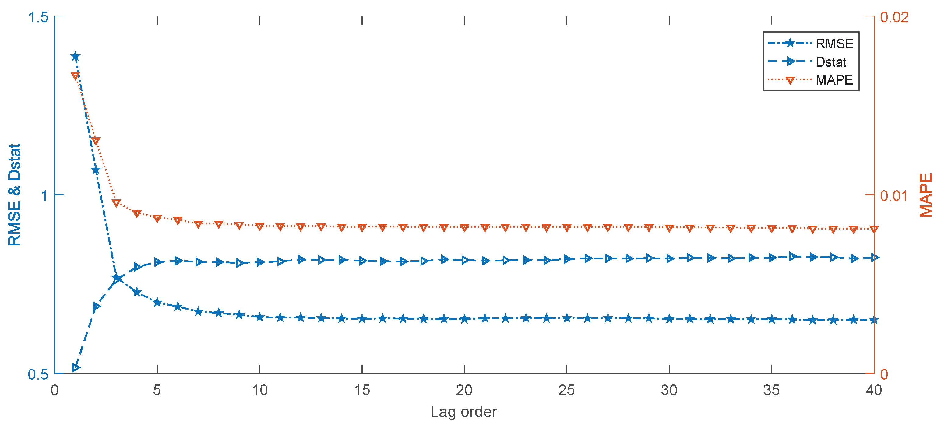
In the above experiments, we use a fixed lag order of six to compare the models, as suggested by [43]. To further analyze the impact of the lag order on the proposed EEMD-SBL-ADD model, we conducted one-step-ahead forecasting on WTI crude oil prices with the lag order in the range of 1–40. The results are shown in Figure 4. It can be seen that when the lag order is not larger than six, the performance of the EEMD-SBL-ADD improves dramatically with the increase of lag in terms of MAPE, RMSE and Dstat. Then, MAPE and RMSE slightly improve with the lag order increases from 7–11, while Dstat keeps stable with the same lag orders. Furthermore, none of the metrics will clearly improve any more when the lag order is larger than 11. The experimental results also confirm that the lag order of six is good enough for forecasting crude oil prices. However, for the proposed EEMD-SBL-ADD model, the performance can be further improved by selecting 11 as the lag order. It can be seen that the proposed EEMD-SBL-ADD is capable of selecting a suitable lag order for forecasting crude oil prices.

4.5.3. The Impact of SBL’s Parameter Settings

The scalar trade-off parameter $\lambda$ to balance sparsity and data fit and the maximum number of iteration n in SBL have slight impacts on the forecasting performance. In most cases, SBL with default values for these two parameters (e.g., $\lambda =0.0004$ and $n=600$) can achieve satisfactory results. To further demonstrate this, we study the impact of these parameters for forecasting crude oil prices. We conduct the experiments on WTI with one-step-ahead forecasting. First, we fix $\lambda =0.0004$ and run EEMD-SBL-ADD with a variable maximum number of iterations n in the range of $\{50,100,200,300,400,500,600,700,800,900,1000\}$. The results are shown in Figure 5. Second, we fix $n=600$ and run the experiments with variable $\lambda$ in the range of $\{0.0001,0.0002,0.0004,0.001,0.002,0.004,0.008,0.016,0.032,0.064,0.128\}$, and the results are shown in Figure 6.

It can be seen that with fixed $\lambda =0.0004$, when the maximum number of iteration n varies from 50–10,000, the results in terms of MAPE, RMSE and Dstat are all very stable, showing that the proposed EEMD-SBL-ADD is not sensitive to the maximum number of iterations. Similarly, when n is fixed at 600 and $\lambda$ varies from 0.0001–0.002, the results also keep almost the same, while when it varies from 0.004–0.128, the results gradually become worse. All the results demonstrate that the proposed EEMD-SBL-ADD is not sensitive to the parameter settings. Even if we use default settings (e.g., $\lambda =0.0004$ and $iteration=600$), it can achieve satisfactory results.

5. Conclusions

Accurate forecasting of crude oil prices is a challenging task because of its attributes of nonlinearity and nonstationarity. Traditional methods including statistical methods and AI-based models usually cannot achieve satisfactory results when the forecasting is performed on raw crude oil prices. Motivated by the strategy of “divide and conquer”, to cope with this issue, this paper proposes a novel model integrating EEMD, SBL and addition (namely EEMD-SBL-ADD) for forecasting crude oil prices, following the “decomposition and ensemble” framework. In the phase of decomposition, EEMD is used to decompose the raw price into several components, and each component shows simpler characteristics compared with the raw prices. Then, this paper uses SBL to forecast each component individually. Finally, the predicted results of all components are aggregated by the simple operation of addition. To demonstrate the performance of the proposed model, we compare it with some state-of-the-art methods on crude oil prices from the popular markets of WTI and Brent with different horizons. This is the first time that non-kernel trick SBL has been applied to forecasting crude oil prices. From the experimental results, some conclusions can be drawn: (1) as an AI model, SBL outperforms other models in forecasting crude oil prices with raw data, demonstrating its power for time series forecasting; (2) the AI-based ensemble approaches are superior to their counterpart single models, indicating that the decomposed component is capable of better representing the characteristics of crude oil prices; in addition, EEMD outperforms EMD for decomposition; (3) the EEMD-SBL-ADD outperforms any other competitive models in terms of the evaluation criteria, showing its promise for forecasting crude oil prices.

One limitation of the proposed EEMD-SBL-ADD model is that all components are predicted using SBL. In fact, among the components, each component shows some different characteristics. For example, some components are of high frequency, while others show low frequency. An ideal model should use different predictors for high- and low-frequency components, respectively. This is one of the extended research directions in our future work. Another interesting direction is to apply the proposed approach to forecasting some other forms of energy, such as wind speed and electricity load. We will also use SBL to perform multivariate forecasting on crude oil prices and to find significant measures to analyze time-varying persistence in crude oil prices, due to the sparsity of SBL.

References

- British Petroleum. 2017 Energy Outlook. 2017. Available online: https://www.bp.com/content/dam/bp/pdf/energy-economics/energy-outlook-2017/bp-energy-outlook-2017.pdf (accessed on 28 July 2017).
- Wang, Y.; Wei, Y.; Wu, C. Detrended fluctuation analysis on spot and futures markets of West Texas Intermediate crude oil. Phys. A Stat. Mech. Appl. 2011, 390, 864–875. [Google Scholar] [CrossRef]
- He, K.J.; Yu, L.; Lai, K.K. Crude oil price analysis and forecasting using wavelet decomposed ensemble model. Energy 2012, 46, 564–574. [Google Scholar] [CrossRef]
- Yu, L.A.; Dai, W.; Tang, L. A novel decomposition ensemble model with extended extreme learning machine for crude oil price forecasting. Eng. Appl. Artif. Intell. 2016, 47, 110–121. [Google Scholar] [CrossRef]
- Li, T.; Zhou, M.; Guo, C.; Luo, M.; Wu, J.; Pan, F.; Tao, Q.; He, T. Forecasting Crude Oil Price Using EEMD and RVM with Adaptive PSO-Based Kernels. Energies 2016, 9, 1014. [Google Scholar] [CrossRef]
- Baumeister, C.; Kilian, L. Real-time forecasts of the real price of oil. J. Bus. Econ. Stat. 2012, 30, 326–336. [Google Scholar] [CrossRef]
- Hooper, V.J.; Ng, K.; Reeves, J.J. Quarterly beta forecasting: An evaluation. Int. J. Forecast. 2008, 24, 480–489. [Google Scholar] [CrossRef]
- Murat, A.; Tokat, E. Forecasting oil price movements with crack spread futures. Energy Econ. 2009, 31, 85–90. [Google Scholar] [CrossRef]
- Abledu, G.K.; Agbodah, K. Stochastic Forecasting and Modelling of Volatility of Oil Prices in Ghana using ARIMA Time series model. Eur. J. Bus. Manag. 2012, 4, 122–131. [Google Scholar]
- Ahmed, R.A.; Shabri, A.B. Daily crude oil price forecasting model using arima, generalized autoregressive conditional heteroscedastic and support vector machines. Am. J. Appl. Sci. 2014, 11, 425. [Google Scholar] [CrossRef]
- Morana, C. A semiparametric approach to short-term oil price forecasting. Energy Econ. 2001, 23, 325–338. [Google Scholar] [CrossRef]
- Arouri, M.E.H.; Lahiani, A.; Lévy, A.; Nguyen, D.K. Forecasting the conditional volatility of oil spot and futures prices with structural breaks and long memory models. Energy Econ. 2012, 34, 283–293. [Google Scholar] [CrossRef]
- Wang, Y.; Wu, C. Forecasting energy market volatility using GARCH models: Can multivariate models beat univariate models? Energy Econ. 2012, 34, 2167–2181. [Google Scholar] [CrossRef]
- Mohammadi, H.; Su, L. International evidence on crude oil price dynamics: Applications of ARIMA-GARCH models. Energy Econ. 2010, 32, 1001–1008. [Google Scholar] [CrossRef]
- Kilian, L. Not all oil price shocks are alike: Disentangling demand and supply shocks in the crude oil market. Am. Econ. Rev. 2009, 99, 1053–1069. [Google Scholar] [CrossRef]
- Kruse, R.; Wegener, C. Time-varying persistence in real oil prices and its determinant. 2017; unpublished. [Google Scholar]
- Mirmirani, S.; Li, H.C. A comparison of VAR and neural networks with genetic algorithm in forecasting price of oil. Adv. Econ. 2004, 19, 203–223. [Google Scholar]
- Azadeh, A.; Moghaddam, M.; Khakzad, M.; Ebrahimipour, V. A flexible neural network-fuzzy mathematical programming algorithm for improvement of oil price estimation and forecasting. Comput. Ind. Eng. 2012, 62, 421–430. [Google Scholar] [CrossRef]
- Kristjanpoller, W.; Minutolo, M.C. Forecasting volatility of oil price using an artificial neural network- GARCH model. Exp. Syst. Appl. 2016, 65, 233–241. [Google Scholar] [CrossRef]
- Jammazi, R.; Aloui, C. Crude oil price forecasting: Experimental evidence from wavelet decomposition and neural network modeling. Energy Econ. 2012, 34, 828–841. [Google Scholar] [CrossRef]
- Tang, M.; Zhang, J. A multiple adaptive wavelet recurrent neural network model to analyze crude oil prices. J. Econ. Bus. 2012, 64, 275–286. [Google Scholar]
- Tipping, M.E. Sparse Bayesian learning and the relevance vector machine. J. Mach. Learn. Res. 2001, 1, 211–244. [Google Scholar]
- Wipf, D.P.; Rao, B.D. Sparse Bayesian learning for basis selection. IEEE Trans. Signal Process. 2004, 52, 2153–2164. [Google Scholar] [CrossRef]
- Zhang, Z.; Rao, B.D. Sparse signal recovery with temporally correlated source vectors using sparse Bayesian learning. IEEE J. Sel. Top. Signal Process. 2011, 5, 912–926. [Google Scholar] [CrossRef]
- Zhang, Z.; Jung, T.P.; Makeig, S.; Rao, B.D. Compressed sensing for energy-efficient wireless telemonitoring of noninvasive fetal ECG via block sparse Bayesian learning. IEEE Trans. Biomed. Eng. 2013, 60, 300–309. [Google Scholar] [CrossRef] [PubMed]
- Li, T.; Zhang, Z. Robust face recognition via block sparse bayesian learning. Math. Probl. Eng. 2013, 2013, 695976. [Google Scholar] [CrossRef]
- Yu, L.A.; Wang, S.Y.; Lai, K.K. Forecasting crude oil price with an EMD-based neural network ensemble learning paradigm. Energy Econ. 2008, 30, 2623–2635. [Google Scholar] [CrossRef]
- Yu, L.; Wang, Z.; Tang, L. A decomposition—Ensemble model with data-characteristic-driven reconstruction for crude oil price forecasting. Appl. Energy 2015, 156, 251–267. [Google Scholar] [CrossRef]
- Bao, Y.; Wang, H.; Wang, B. Short-term wind power prediction using differential EMD and relevance vector machine. Neural Comput. Appl. 2014, 25, 283–289. [Google Scholar] [CrossRef]
- Alamaniotis, M.; Ikonomopoulos, A.; Alamaniotis, A.; Bargiotas, D.; Tsoukalas, L.H. Day-ahead electricity price forecasting using optimized multiple-regression of relevance vector machines. In Proceedings of the 8th Mediterranean Conference on Power Generation, Transmission, Distribution and Energy Conversion (MEDPOWER 2012), Cagliari, Italy, 1–3 October 2012; pp. 1–5. [Google Scholar]
- Huang, N.E.; Shen, Z.; Long, S.R. A new view of nonlinear water waves: The Hilbert Spectrum 1. Ann. Rev. Fluid Mech. 1999, 31, 417–457. [Google Scholar] [CrossRef]
- Wu, Z.; Huang, N.E. Ensemble empirical mode decomposition: A noise-assisted data analysis method. Adv. Adapt. Data Anal. 2009, 1, 1–41. [Google Scholar] [CrossRef]
- Zhu, B.; Wei, Y. Carbon price forecasting with a novel hybrid ARIMA and least squares support vector machines methodology. Omega 2013, 41, 517–524. [Google Scholar] [CrossRef]
- Tolambiya, A.; Kalra, P.K. Relevance vector machine with adaptive wavelet kernels for efficient image coding. Neurocomputing 2010, 73, 1417–1424. [Google Scholar] [CrossRef]
- Tzikas, D.; Likas, A.; Galatsanos, N. Large scale multikernel relevance vector machine for object detection. Int. J. Artif. Intell. Tools 2007, 16, 967–979. [Google Scholar] [CrossRef]
- Yan, X.F.; Sun, S.J.; Wang, J.; Feng, J. Oil production prediction of oil field based on primal twin relevance vector regression algorithm. Inf. Int. Interdiscip. J. 2012, 15, 4313–4320. [Google Scholar]
- Zhang, Y.S.; Liu, B.Y.; Zhang, Z.L. Combining ensemble empirical mode decomposition with spectrum subtraction technique for heart rate monitoring using wrist-type photoplethysmography. Biomed. Signal Process. Control 2015, 21, 119–125. [Google Scholar] [CrossRef]
- Zhou, Y.; Zhao, H.M.; Pan, X.Y.; Shang, L. Deception detecting from speech signal using relevance vector machine and non-linear dynamics features. Neurocomputing 2015, 151, 1042–1052. [Google Scholar] [CrossRef]
- Widodo, A.; Kim, E.Y.; Son, J.D.; Yang, B.S.; Tan, A.C.; Gu, D.S.; Choi, B.K.; Mathew, J. Fault diagnosis of low speed bearing based on relevance vector machine and support vector machine. Exp. Syst. Appl. 2009, 36, 7252–7261. [Google Scholar] [CrossRef]
- Zhang, Z.; Rao, B.D. Extension of SBL algorithms for the recovery of block sparse signals with intra-block correlation. IEEE Trans. Signal Process. 2013, 61, 2009–2015. [Google Scholar] [CrossRef]
- Hansen, P.R.; Lunde, A.; Nason, J.M. The model confidence set. Econometrica 2011, 79, 453–497. [Google Scholar] [CrossRef]
- Yu, L.; Dai, W.; Tang, L.; Wu, J. A hybrid grid-GA-based LSSVR learning paradigm for crude oil price forecasting. Neural Comput. Appl. 2016, 27, 2193–2215. [Google Scholar] [CrossRef]
- Yu, L.; Zhao, Y.; Tang, L. A compressed sensing based AI learning paradigm for crude oil price forecasting. Energy Econ. 2014, 46, 236–245. [Google Scholar] [CrossRef]
Figure 1.
Flowchart for the proposed approach. EEMD: ensemble empirical mode decomposition; IMF: intrinsic mode function; SBL: sparse Bayesian learning.
Figure 2.
The original data and corresponding components decomposed by EEMD of West Texas Intermediate (WTI) crude oil prices. IMF: intrinsic mode function.
Figure 3.
The original data and corresponding components decomposed by EEMD of Brent crude oil prices. IMF: intrinsic mode function.
Figure 4.
The impact of lag on WTI crude oil prices with one-step-ahead forecasting.
Figure 5.
The impact of the variable maximum number of iteration n along with fixed on WTI crude oil prices with one-step-ahead forecasting.
Figure 6.
The impact of variable along with the fixed maximum number of iteration on WTI crude oil prices with one-step-ahead forecasting.