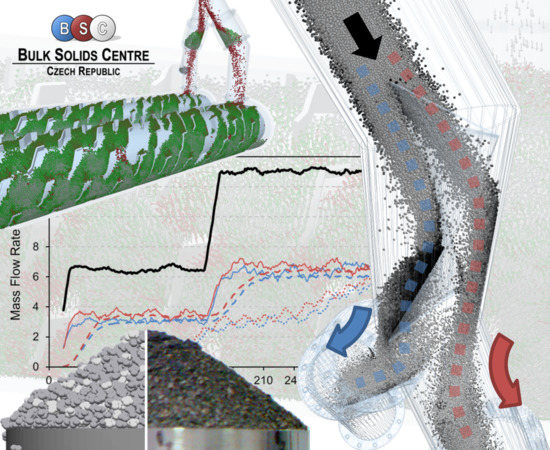
Analysis and Optimization of Material Flow inside the System of Rotary Coolers and Intake Pipeline via Discrete Element Method Modelling

Abstract

There is hardly any industry that does not use transport, storage, and processing of particulate solids in its production process. In the past, all device designs were based on empirical relationships or the designer’s experience. In the field of particulate solids, however, the discrete element method (DEM) has been increasingly used in recent years. This study shows how this simulation tool can be used in practice. More specifically, in dealing with operating problems with a rotary cooler which ensures the transport and cooling of the hot fly ash generated by combustion in fluidized bed boilers. For the given operating conditions, an analysis of the current cooling design was carried out, consisting of a non-standard intake pipeline, which divides and supplies the material to two rotary coolers. The study revealed shortcomings in both the pipeline design and the cooler design. The material was unevenly dispensed between the two coolers, which combined with the limited transport capacity of the coolers, led to overflowing and congestion of the whole system. Therefore, after visualization of the material flow and export of the necessary data using DEM design measures to mitigate these unwanted phenomena were carried out.

1. Introduction

Market pressure forces companies to develop increasingly optimized products with regard to transport efficiency, environmental impacts, and material and labor savings. Nowadays, to propose innovative processes, industries require the use of sophisticated simulation techniques. Some of these are based in the discrete element method (DEM), which use virtual models to simulate the dynamic flow of particulate solids [1] in transport, handling, storage, and process systems [2]. At present, DEM is drawing the attention of many designers and manufacturers of equipment as well as process engineers. It has become a useful tool to analyze industrial processes [3]. It makes it possible to test the basic functionality of devices [4] and their structural configurations before prototyping or to optimize existing equipment, resulting in considerable economic, time, labor, and material savings. One of the challenges of modeling the processes of particulate solids is the creation of a mathematical model for the bulk material itself, whose behavior is influenced by a great number of factors. The behavior of powders and bulk materials depends on external and internal factors that influence their bulk density, internal and external angle of friction, angle of repose, cohesiveness, particle morphology and granulometry, flowability, and many other parameters [5].

Since the current requirements go beyond the simple transportation of materials from A to B but rather require a combination of the transportation with processes (i.e., drying, cooling, sorting, etc.), DEM opens up new possibilities in design and process optimization avoiding design errors before implementation. Recently, there has been a tendency to link the DEM method to other numerical simulation methods such ascomputational fluid dynamics (CFD) [6], finite element method (FEM) [7] or multi-body dynamics (MBD) to solve more complex problems [8]. Development and improvement of any structure is a time-consuming effort, but it is essential for business competitiveness and product sales. The using of numerical methods for study and optimization is very common and desirable today. These numerical techniques extend the possibilities of optimizing the construction elements of the conveyors as well as in the area of critical loads (stress) studies on the transport equipment [9]. In case of material flow through pneumatic transport systems, numerical methods are applied in the areas of new applications and designs of complex multiphase flow situations [10]. New theoretical and numerical approaches can be used to predict and evaluate possible safety risks during transport [11]. In the field of storage, it is possible to use numerical methods for solving complex tasks of flow of particulates from silos with respect to acting wall pressures, speed profiles, and particle shape [12]. It can be very challenging for some companies to design the correct pipeline for their equipment. This research motivates industrial practitioners and engineers to adopt DEM as an important tool for designing and troubleshooting of equipment. There are many processes and handling operations with particulates in the energy industry. The DEM can be used in wide scale of applications, i.e., coal and fly ash handling, grinding processes, storage bins design, etc. Bai and He (2015) published a study on the effect of coal loads on kinetic energy of balls for ball mills where the kinetic energy of grinding balls was optimized [13].

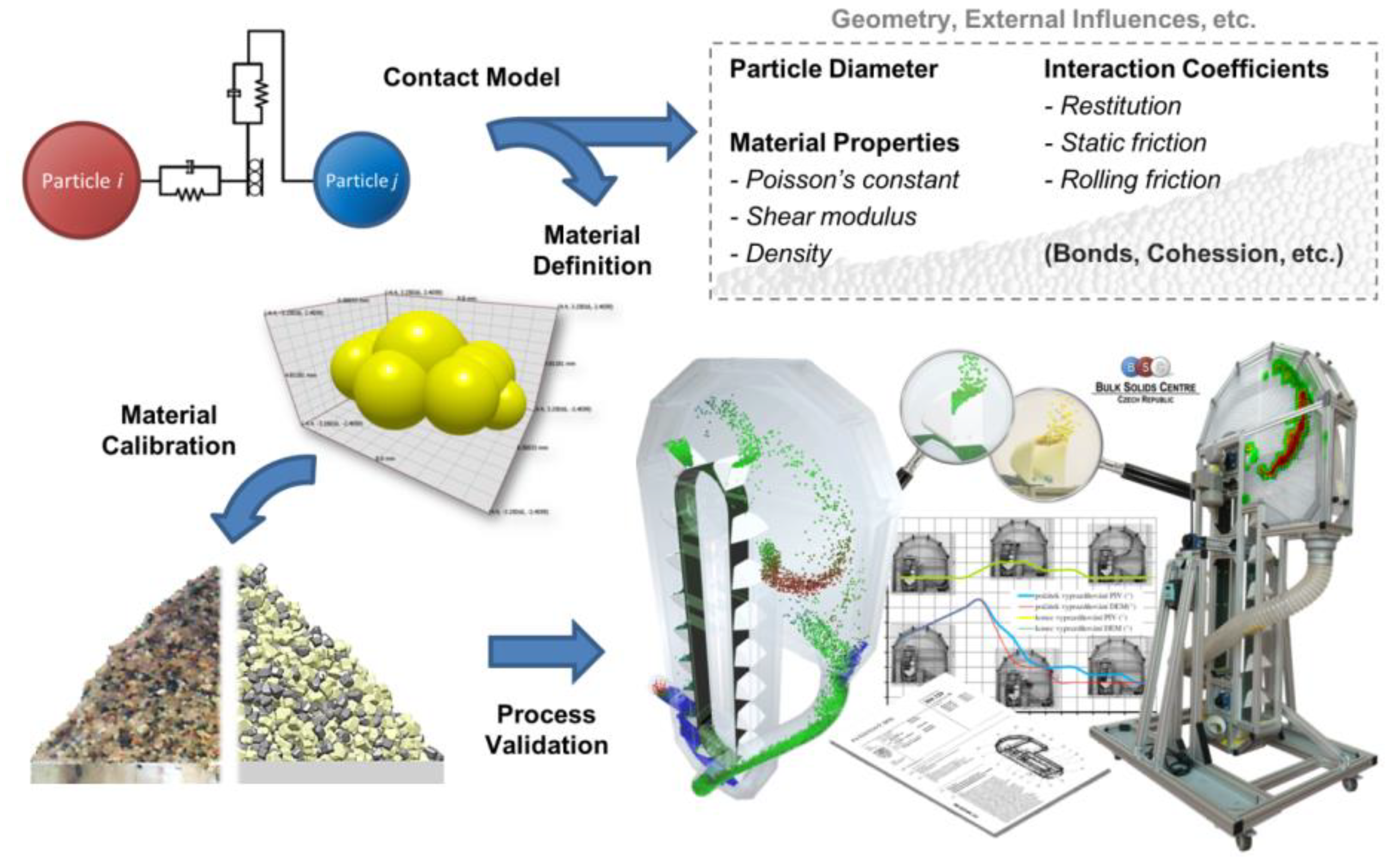
2. Theoretical Background

The basic principle of the DEM modeling procedure is based on a particle contact model, which is defined by parameters such as particle diameter, Poisson’s ratio, interaction coefficients and density. The particle simulation model defined in this way is calibrated based on experimental data. Finally, the data from the experimental and simulation model of the application (e.g., conveyor) is verified. The diagram of the modeling procedure is shown in Figure 1. The basic material optimization with Hertz-Mindlin contact model through the angle of repose has been performed in this study. In the next step, simulation with the original state of coolers was performed. This simulation corresponded with the behavior of the real equipment. Therefore, some geometric adjustments has been designed and tested by simulation again. Mass flow rates and particle trajectories in different parts of the cooling system were understood thanks to this study. The goal of this study is to present the principle and optimization process via DEM modelling in industrial scale equipment, where there are tonnes of material transported or handled per hour.

Originally published by Cundall and Strack in 1979, the discrete element method has become over time a commonly used numerical tool for particle modeling [14]. In DEM models, the particulate material is modeled as an assembly of particles interacting with each other or with parts of the equipment or facilities where present (moving paddles of cooling conveyors, walls of hoppers, silos, and pipelines, etc.). The macroscopic behavior of particles is due to the microscopic interactions between the particles themselves and between the particles and boundary conditions. The determination of trajectory and velocity of particles is performed in discrete time steps. Much of the information about this behavior, such as collision frequency or interaction forces, is based on these calculations. Theoretical particle movement through other particles shows flow mechanisms at the scale and level of detail that would be otherwise very difficult to achieve by experimental means.

Reliability and the nature of discrete models depend entirely on simplifying many physical properties of particulate solids. These properties need to be described in DEM using several simple interaction parameters. Such simplifications are necessary and are widely used to solve complex problems within reasonable timeframes. In the literature, there has been little work done in verifying the flow of particulate solids in the global scale of the entire technology. If DEM is to become an equally important design tool, such as FEM or CFD numerical modeling, it is absolutely necessary to verify the capabilities of DEM by simulations, i.e., to provide insight into the interaction mechanisms in installations where it is difficult to monitor flow, obtain measurements or quantify its performance [15].

A number of problems with gravity tables are solved within gravity separation processes, e.g., a slope of the table or air intake [16]. Additive technologies address geometric optimization to improve the quality of the applied layer [17]. In the sorting areas, the optimal setting of the operating device is solved [18]. Mixing processes need to be investigated and compared with the properties of mixed materials [19]. It is necessary and possible to optimize new production technologies and equipment [20] in industry and engineering with regard to service life [21]. For example, there are problems with the flow of particulate solids when storing materials in silos [22] or during pneumatic transportation in pipelines [23]. In the pharmaceutical and chemical industry, material segregation or inappropriate distribution of the active substance may occur during processing. In all these industries, DEM can provide significant information for problem-solving [24]. The study of bulk materials can be carried out either as a continuum or as a particle conglomerate. As for the latter approach, a great deal of work has been published in recent years on the issue of physical interactions of individual particles [25]. A number of studies of micro-mechanical interactions between particles have been carried out, such as the stress state inside the material or the distribution of internal forces within the assembly. However, due to the lack of sufficiently sensitive measuring experimental equipment, mathematical models or computational simulations, approaches to the extensive problems of bulk mechanics have not been explored or extended [26].

As the world recedes gradually out off coal as a source of energy, cleaner and more competitive energy sources, such as renewable energy sources, will emerge. From biomass and waste, 13% of the world’s total energy consumption is projected to be from coal in 2040 [27]. Coal has experienced the greatest development as an energy source in 2000–2012. In addition, the use of oil and natural gas has experienced growth, followed by hydropower and renewable energy sources. The use of nuclear energy decreased in recent years because of nuclear disasters risk. Therefore, it is necessary to construct all energy devices with maximum reliability in terms of their number and importance. This study presents innovative ways of using the DEM method in optimizing a rotary cooler. Such cooler is installed under a fluidized bed boiler of a power plant and a heating plant and serves for cooling and transporting of hot fly ash from the boiler to waste disposal. A comprehensive solution of material flow prediction and similar technological (cooling) processes includes the determination of flow, mechanical, physical, granulometric, and thermal properties of the conveyed particulate solids [28]. Various methods of determining the thermal conductivity of powders [29], which can be generally used in designing coolers, in calculation of the heat exchange surface, and the material retention time in the cooler, especially in the combination of CFD–DEM numerical methods [30,31,32], can be found in the literature. This study focuses on the shape optimization of the intake pipeline and the active parts of the cooling system. To solve the malfunction of one of two devices that are identical, an optimized solution has been found to ensure continuous operation of the device via DEM modeling in a comparative way.

The DEM algorithm generally starts with placing the particles in the system. For the calculation of contact force, EDEM performs detection of contacts to determine whether the individual particles interact with each other in the current time step. Contact detection is time-consuming and requires substantial computing power. After contact detection is completed, the total force applied to each particle is determined and therefore the translational, as well as rotational motion, can be determined by integrating the Newton Equation (1) and its equivalent (2). Between each time step of the calculation process, the particles are moved based on the speed and acceleration calculated in the previous time step. Contacts are then used to calculate the reaction forces acting on each particle. This force determines its speed and acceleration in the next time interval. The resulting force and torque represent the sum of all the forces and torques applied to each particle, including gravity, fluid flow, magnetic fields, electrostatic fields, external forces and so on.

In this study forces and torques caused by gravity, contacts, static, and rolling friction are considered. Therefore, the Newton equations of motion of the particle i in contact with the particle j the following form:

$${\mathrm{m}}_{\mathrm{i}}\frac{{\mathrm{d}\mathrm{v}}_{\mathrm{i}}}{\mathrm{d}\mathrm{t}}=\sum \left({\mathrm{F}}_{\mathrm{i}\mathrm{j}}^{\mathrm{n}}{+\mathrm{F}}_{\mathrm{i}\mathrm{j}}^{\mathrm{t}}\right){+\mathrm{m}}_{\mathrm{i}}\mathrm{g}$$

(1)

$${\mathrm{I}}_{\mathrm{i}}\frac{{\mathrm{d}\mathsf{\omega }}_{\mathrm{i}}}{\mathrm{d}\mathrm{t}}=\sum \left({\mathrm{R}\mathrm{V}}_{\mathrm{i}}\times {\mathrm{F}}_{\mathrm{i}\mathrm{j}}^{\mathrm{t}}-{\mathsf{\tau }}_{\mathrm{i}\mathrm{j}}^{\mathrm{r}}\right)$$

(2)

where m_i, I_i, v_i and ω_i are the mass, the moment of inertia, the speed of movement and the angular velocity of the rotation of the particle i. F_ijⁿ and F_ij^t is the normal and tangential force induced by contact of particle i with particle j in the current time step. RV_i represents the reaction vector between the center of the particle i and the contact point where the force F_ij^t is acting.

The contact model is necessary to evaluate the mutual forces between the particles themselves but also between the particles and other solid bodies in their contact with each other. There are a number of different contact models, but there is no general rule as to which contact model is the best as these models are not equivalent and address different particle contact properties. For example, models based on Hertz theory consider particles in which the contacts lead to nonlinear elastic deformation, whereas the model of the linear spring damping assumes that this deformation is rather viscoelastic. All these models depend on the parameters whose values must be included in the input settings. The basic input values are the radius of the particles R, particle density ρ, Young’s modulus E (shear modulus G), and interaction coefficients.

Tsuji et al. (1992) [33] proposed a nonlinear contact model based on the adaptation of the original model proposed by Cundall and Strack. This currently widely used Hertz-Mindlin model is described by Equations (3) and (4). This model included a non-linear member based on Hertz theory for normal contact. For tangential contact, Tsuji suggested to include viscous dissipation. The modified contact model, therefore, is as follows:

$${\mathrm{F}}_{\mathrm{ij}}^{\mathrm{n}}=\left(-{\mathrm{k}}_{\mathrm{n}}{\mathsf{\delta }}_{\mathrm{ij}}^{\mathrm{n}\raisebox{1ex}{$3$}\!\left/ \!\raisebox{-1ex}{$2$}\right.}-{\mathsf{\eta }}_{\mathrm{n}}\left({\mathrm{v}}_{\mathrm{ij}}^{\mathrm{sh}}·{\mathrm{n}}_{\mathrm{ij}}\right){\mathrm{n}}_{\mathrm{ij}}\right)$$

(3)

$${\mathrm{F}}_{\mathrm{ij}}^{\mathrm{t}}=\left(-{\mathrm{k}}_{\mathrm{t}}{\mathsf{\delta }}_{\mathrm{ij}}^{\mathrm{t}}-{\mathsf{\eta }}_{\mathrm{t}}{\mathrm{v}}_{\mathrm{ij}}^{\mathrm{t}}\right)$$

(4)

Slip speed v_ij^sh is replaced with relative tangent speed v_ij^t. Sufficiently high tangential forces cause the particles to slide relative to one another or to the surfaces with which they come in contact. EDEM software offers several different contact models and, if necessary, also the creation of user-defined models. Modified contact model Hertz-Mindlin represents the EDEM default contact model and is based on the model proposed by Tsuji et al. In the Hertz-Mindlin contact model, during the collision of the particle i with particle j the normal force F_ijⁿ acting on each particle is given by:

$${\mathrm{F}}_{\mathrm{ij}}^{\mathrm{n}}=-\frac{4}{3}{\mathrm{E}}^{*}\sqrt{{\mathrm{R}}^{*}}{\mathsf{\delta }}_{\mathrm{ij}}^{\mathrm{n}\raisebox{1ex}{$3$}\!\left/ \!\raisebox{-1ex}{$2$}\right.}-2\sqrt{\frac{5}{6}}\mathsf{\psi }\sqrt{{\mathrm{k}}_{\mathrm{n}}{\mathrm{m}}^{*}}{\mathrm{v}}_{\mathrm{ij}}^{\mathrm{n}}$$

(5)

where E* is equivalent to Young’s module of two colliding particles, R* is an equivalent contact radius, δ_ijⁿ is normal displacement of particles by normal force, m* is the equivalent mass of particles, v_ijⁿ is the normal component of relative velocity, and the normal contact stiffness is k_n = 2E*(Rδ_n)^0.5. Damping coefficient ψ is a function of the coefficient of restitution e and ranges from 0 (absolutely viscous) to 1 (absolutely elastic). F_ij^t depends on tangential displacement δ_ij^t, relative tangential velocity v_ij^t as well as on tangential stiffness k_t = 8G*(Rδ_t)^0.5. The tangential force is limited by the Coulomb’s law of friction.

$${\mathrm{F}}_{\mathrm{ij}}^{\mathrm{t}}={-\mathrm{k}}_{\mathrm{t}}{\mathsf{\delta }}_{\mathrm{ij}}^{\mathrm{t}}-2\sqrt{\frac{5}{6}}\mathsf{\psi }\sqrt{{\mathrm{k}}_{\mathrm{t}}\mathrm{m}}{\mathrm{v}}_{\mathrm{ij}}^{\mathrm{t}}$$

(6)

Damping coefficient ψ is a function of the coefficient of restitution e and is defined as:

$$\mathsf{\psi }=-\frac{\ln \mathrm{e}}{\sqrt{{\left(\ln \mathrm{e}\right)}^2+{\mathsf{\pi }}^2}}$$

(7)

In the default EDEM Hertz-Mindlin contact model, the coefficient of restitution for the given case is constant with respect to the impact velocity, provided that other parameters are also constant. The two particles i and j have the equivalent contact radius R*, equivalent mass m*, equivalent Young’s Module E* and shear module G* defined as follows:

$${\mathrm{R}}^{*}={\left(\frac{1}{{\mathrm{R}}_{\mathrm{i}}}+\frac{1}{{\mathrm{R}}_{\mathrm{j}}}\right)}^{-1}=\frac{{\mathrm{R}}_{\mathrm{i}}{\mathrm{R}}_{\mathrm{j}}}{{\mathrm{R}}_{\mathrm{i}}{+\mathrm{R}}_{\mathrm{j}}}$$

(8)

$${\mathrm{m}}^{*}={\left(\frac{1}{{\mathrm{m}}_{\mathrm{i}}}+\frac{1}{{\mathrm{m}}_{\mathrm{j}}}\right)}^{-1}=\frac{{\mathrm{m}}_{\mathrm{i}}{\mathrm{m}}_{\mathrm{j}}}{{\mathrm{m}}_{\mathrm{i}}{+\mathrm{m}}_{\mathrm{j}}}$$

(9)

$${\mathrm{E}}^{*}=\left(\frac{{1-\mathsf{\upsilon }}_{\mathrm{i}}}{{\mathrm{E}}_{\mathrm{i}}}+\frac{{1-\mathsf{\upsilon }}_{\mathrm{j}}}{{\mathrm{E}}_{\mathrm{j}}}\right)$$

(10)

$$\frac{1}{{\mathrm{G}}^{*}}=\left(\frac{{2-\mathsf{\upsilon }}_{\mathrm{i}}}{{\mathrm{G}}_{\mathrm{i}}}+\frac{{2-\mathsf{\upsilon }}_{\mathrm{j}}}{{\mathrm{G}}_{\mathrm{j}}}\right)$$

(11)

E_i and E_j is Young’s modulus, G_i and G_j represent a shear modulus, υ_i and υ_j are Poisson’s ratios of particle i and particle j.

If the simple Hertz-Mindlin contact model defined in Equations (5) and (6) is used, the following contact parameters must be defined for the simulation model in EDEM, for both particle–particle contacts and particle–geometry contacts:

• Static friction coefficient μ_s
• Coefficient of rolling friction μ_r
• Coefficient of restitution e

At present, there are a number of sophisticated contact models that can simulate particular systems with a number of different properties. For example, various forms of powdery materials exhibiting plastic or elastic properties, cohesive soils, wet and sticky materials, or even rocks, using solid connections between the particles. Another modern trend is to connect DEM with other numerical methods and software (SW) such as CFD, FEM, MBD, etc. This interconnection improves numerical modeling to such an extent that it is possible to predict pipe wear during pneumatic transport of abrasive materials or to perform stress analysis of transport and mining machines. This, along with ever-increasing computational power opens up unlimited possibilities.

3. Material and Methods

The rotary coolers in this study are used to cool fly ash leaving the boiler. The mechanical–physical properties of the fly ash sample were determined. The objectives of the operational optimization included the assessment of the suitability of the rotary cooler for the process, the assessment of the suitability of the flow path from the fluidized bed boiler through the inlet pipe (Figure 2) into coolers 1 and 2 (Figure 2), and assessment of the possibility of overloading the coolers under the transport capacity of about 13 t/h. The diagram of the whole assembly including the dimensional sketch is shown in Figure 2.

Figure 2 shows all the active elements of the cooler geometry that come into contact with the conveyed material. The 3D computer-aided design (CAD) model represents a simplified form of the real device geometry in real operation. The assembly includes an unusual chute that feeds and distributes the material between the two coolers. Two coolers with an inner diameter of 0.866 m, a length of 6 m with an inclination of 5°, are directly connected to the chute, and the material is transported upwards. The outer shell is cooled by running water. The axial distance between the coolers is 1 m.

3.1. Fly Ash Characterization

Before examining any conveyor, storage or process equipment working with bulk materials, it is first necessary to characterize the material to understand its behavior and specifics. Moreover, characterization of the material is also necessary for the creation of virtual material within the DEM simulation. The fly ash was tested primarily for flow and shear properties that have a major effect on material flow through the device. The Schulze ring shear tester RST-01 was used to determine the angle of internal and wall friction, flowability, and cohesion. In addition, the angle of repose was determined by the method of “piling” where the material is released on a steel bowl of 9 cm in diameter. The material is dispensed from a hopper by a vibratory feeder which end is located above the center of the bowl at a height of 10 cm. The material is dosed as long as the cone is not formed on the entire base of the bowl and until the feed material starts to slip out of the bowl. The angle of repose is sometimes also used to characterize the flowability of powders. Materials with the angle of repose below 30° are classified as free-flowing, 30°–45° as easy-flowing, 45°–55° as cohesive and above 55° as very cohesive to non-flowing materials [34]. According to the results, it is a non-cohesive, easy-flowing material that should not pose any problems during transportation and storage.

3.2. Virtual Material, Geometry Definition, and Contact Model

The DEM model used in this study uses the “soft-sphere” (SSDEM) [35] method originally developed by Cundall and Strack [13]. With this method, the particles in contact are able to withstand small deformations, and these deformations are used to calculate the forces acting between the particles.

Due to computational limits, there are some limitations in current DEM models. Because of the lack of standardized procedures, the determination of the input parameters necessary for simulation can introduce inaccuracies in the results obtained from the numerical models. One of the key issues is still the representation of actual particle shapes and the limited number of particles that can be modeled with a reasonable computational cost. To achieve an acceptable computational cost, most of the DEM simulations include only a limited number of particles with a diameter in the order of millimeters and a maximum particle count of hundreds of thousands. A simple spherical shape and a small number of particles are usually not comparable to real industrial systems, which consist of billions of small irregular particles with wide distributions of particle size. Therefore, a simulation of millions of irregular particles in a complex system cannot reasonably be performed with a single processor. In real industrial operations, some of the observed phenomena (such as mixing, drying, cooling, etc.) may take a long time in minutes and hours. Typical times that can currently be simulated using DEM at this scale are usually shorter. Parallel computing clusters can provide the required level of computational power required for larger DEM simulations. However, as computer hardware continually improves, it should be possible in the future to model complex geometries with a large number of non-spherical particles using readily available multiprocessor units. For instance, EDEM software since its 2017 version supports not only parallel computing on standard central processing unit (CPU) processors but also takes advantage of graphics processing unit (GPU) processors of graphic cards, which has become quite powerful due to computer games. The challenge for DEM modelers is to create simplified models that can be processed at reasonable time frames and are still relevant to real systems that work with millions of irregularly shaped particles with a wide size distribution. The main objective of DEM simulations is to simulate non-spherical particles efficiently. Various complex shape modeling methods have been published, for example, complex particles can be represented in DEM codes as a group of mutually permeable or non-protruding spheres of the same or different radius, ellipsoids or polygons.

Models of non-spherical shapes that represent real particles can be complicated because more sophisticated models of particle interaction are needed rather than a simple contact spherical model. For different types of polygons, contact detection and subsequent computation of forces and torque can be complicated and computationally demanding. Using methods with particles created from a sphere, it is possible to achieve the computation efficiency to detect point contacts and calculation of reaction forces. The disadvantage of this method, however, is that accurate representation of a complex shape requires the clustering of many spherical particles, which in turn requires more computational memory. Another fundamental problem in the development of DEM for real industrial applications is the determination of the input parameters of the particulate material. The simulation input parameters are often not measured, and the values are estimated without proper justification because there is basically no stable method for their determination. To correctly interpret the simulation results, the correct input parameters should be selected, and the simulations should also be validated using experimental tests [36].

Parameters of the virtual material were chosen with respect to the results of the tests performed using the collected samples and by the empirical Equation (12), which indicates the influence of the individual parameters on the angle of repose, according to which the material was subsequently calibrated [37]. To optimize the computation time, a monodisperse virtual material of spherical particles with a diameter of D = 15 mm was chosen. Some different radiuses were tested, but the final particle radius has been chosen for a good compromise between computational time and particle/equipment size ratio. The individual parameters for the virtual material model are shown in

Table 1. Discrete element method (DEM) input parameters; material properties and interaction coefficients for fly ash particles.

Material	Density	Poisson’s Ratio	Young’s Modulus	Coeff. of Restitution	Static Friction	Rolling Friction
	(kg∙m−3)	(-)	(MPa)	(-)	(-)	(°)
Fly ash	7850	0.25	11	0.65	0.8	1.4
Steel	870	0.30	210	0.70	0.9	1.3

. The validation results via angle of repose test are shown in

Table 2. Validation of virtual material via angle of repose test.

	Angle of Repose (°)—Measurement No.								Avg.
	1	2	3	4	5	6	7	8
Experiment	38.5	39.2	38.7	38.4	37.0	38.1	37.1	37.3	38.1
DEM	35.0	43.5	38.8	36.5	37.0	37.0	40.1	40.9	38.6

. The difference between experiment and DEM model is 1.4% in this test. Normally, the total uncertainty of validated simulations is about 5–10% if the quantifiable parameters are compared. Generally, many different tests can be used for validation of model in practice. Unfortunately, in the presented study a calibration at full-scale would not be feasible due to the very high temperature of material. The decisions taken during the whole validation and optimization process have been agreed with experienced practitioners with the intake and the cooling system.

$$\mathrm{AoR}=68.61·{{\mathsf{\mu }}_{\mathrm{s},\mathrm{pp}}}^{0.27}·{{\mathsf{\mu }}_{\mathrm{s},\mathrm{pw}}}^{0.22}·{{\mathsf{\mu }}_{\mathrm{r},\mathrm{pp}}}^{0.06}·{{\mathsf{\mu }}_{\mathrm{r},\mathrm{pw}}}^{0.12}·{\mathrm{D}}^{-0.2}$$

(12)

The basic calibration of the material through angle of repose was performed, and the simulation of the un-modified cooler shows the same process behavior and malfunctions as well as real cooling equipment. By this mean of comparing, the material calibration and geometrical optimization were done for the industrial scale of cooler. Thus, the process is validated for the material, and then a comparative analysis is performed between the original and the optimized solution. The imported 3D CAD model is shown in Figure 3. This figure also shows the location of particle generation (particle factory) as well as seven virtual sensors that export the individual data obtained during the simulation. Sensor 1 (Intake) monitors the input of the material into the chute. The material is then separated and the pipeline continues to the cooler 1 (blue) and cooler 2 (red). Each of the coolers has its own sensor at the inlet, outlet and in the middle part. The analysis of material movement inside the chute and the cooler is described in Section 4.

4. Results and Discussion

In this study, an analysis of existing coolers and chute was first performed using DEM modeling. Once the causes and consequences of operational problems were identified, design measures were proposed, and a simulated operation under the same operating conditions was performed again. These conditions were based on actual operation. First, the material was fed to the chute from the particle factory at a mass flow rate of 6.5 t/h, and the filling of the interior of the cooler and the transport of material divided between the two coolers were monitored. In time T = 150 s, the mass of generated material was increased to the rate of 13 t/h, which caused problems in the actual operation. In all cases, the total simulation time was 330 s. Since this study is focused on the mechanics of the particles, i.e., flow of material throughout the system, the main monitored parameters included mass flow rates of the material in individual parts of the system, the velocity of the particle movement in the various axes of the coordinate system, the number of particle contacts with the heat exchange surface of the cooler as well as the time the material remained in the cooler.

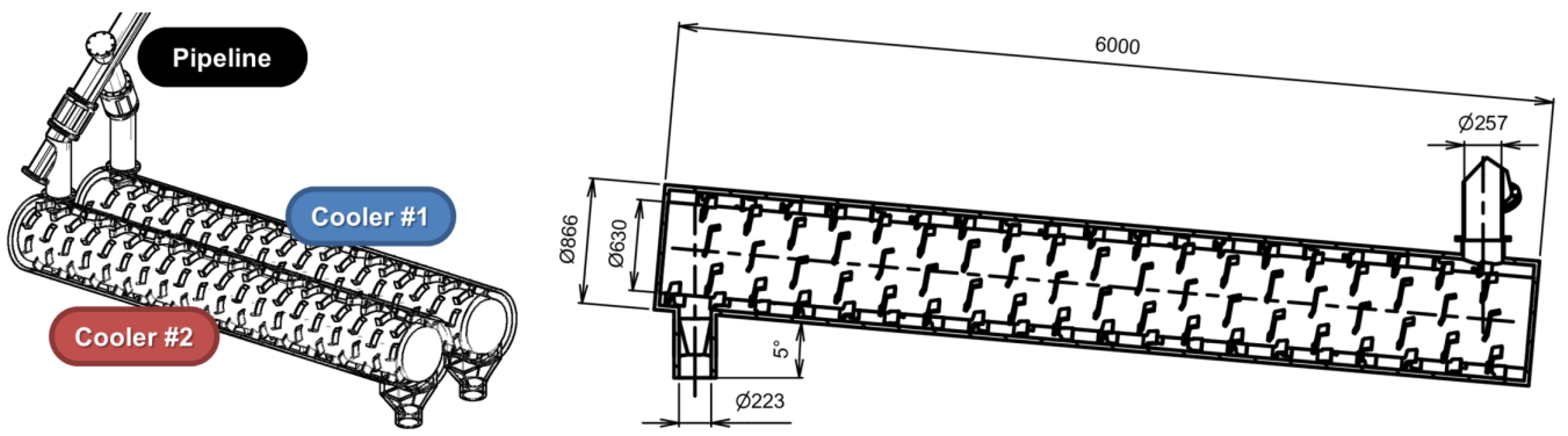
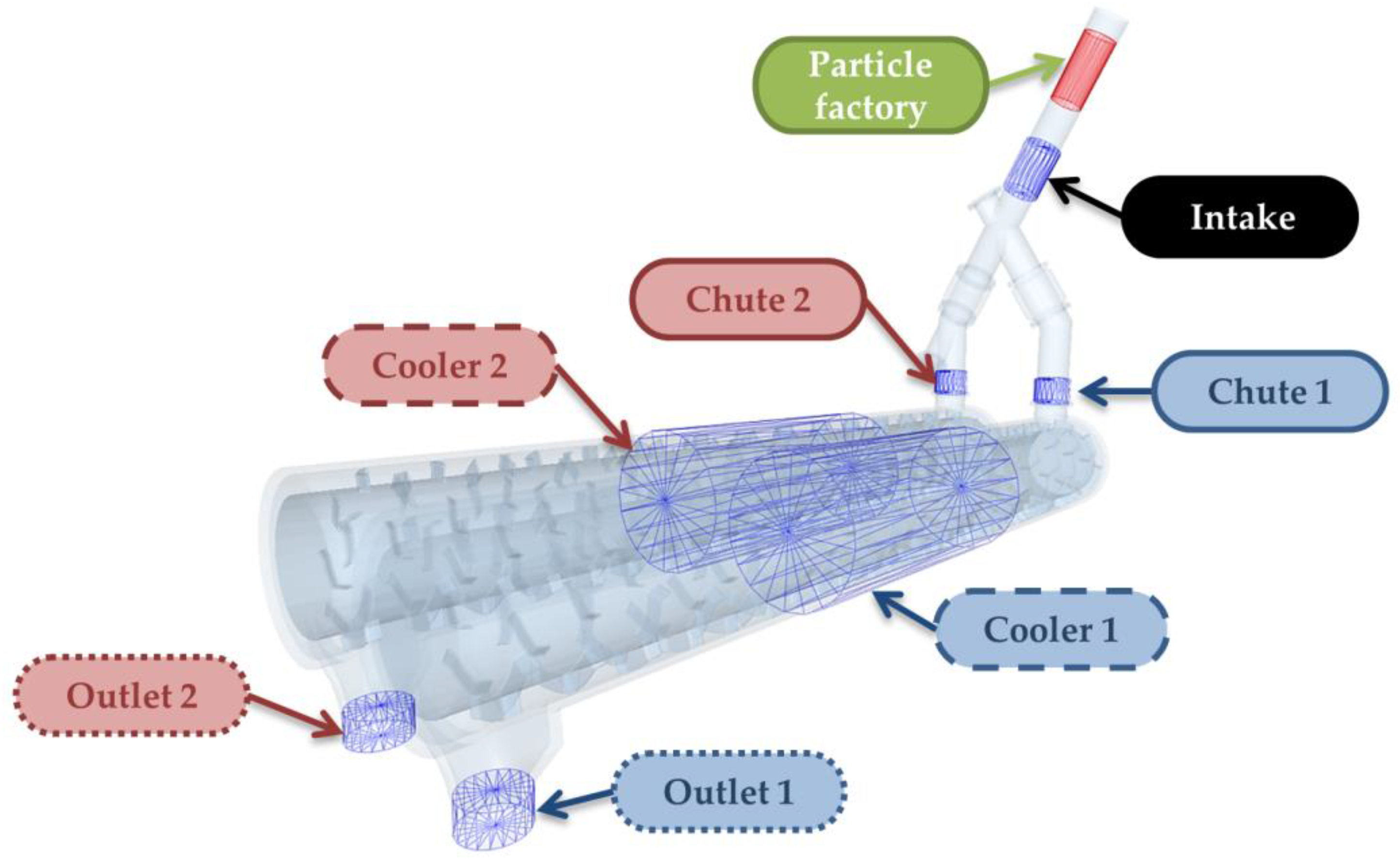
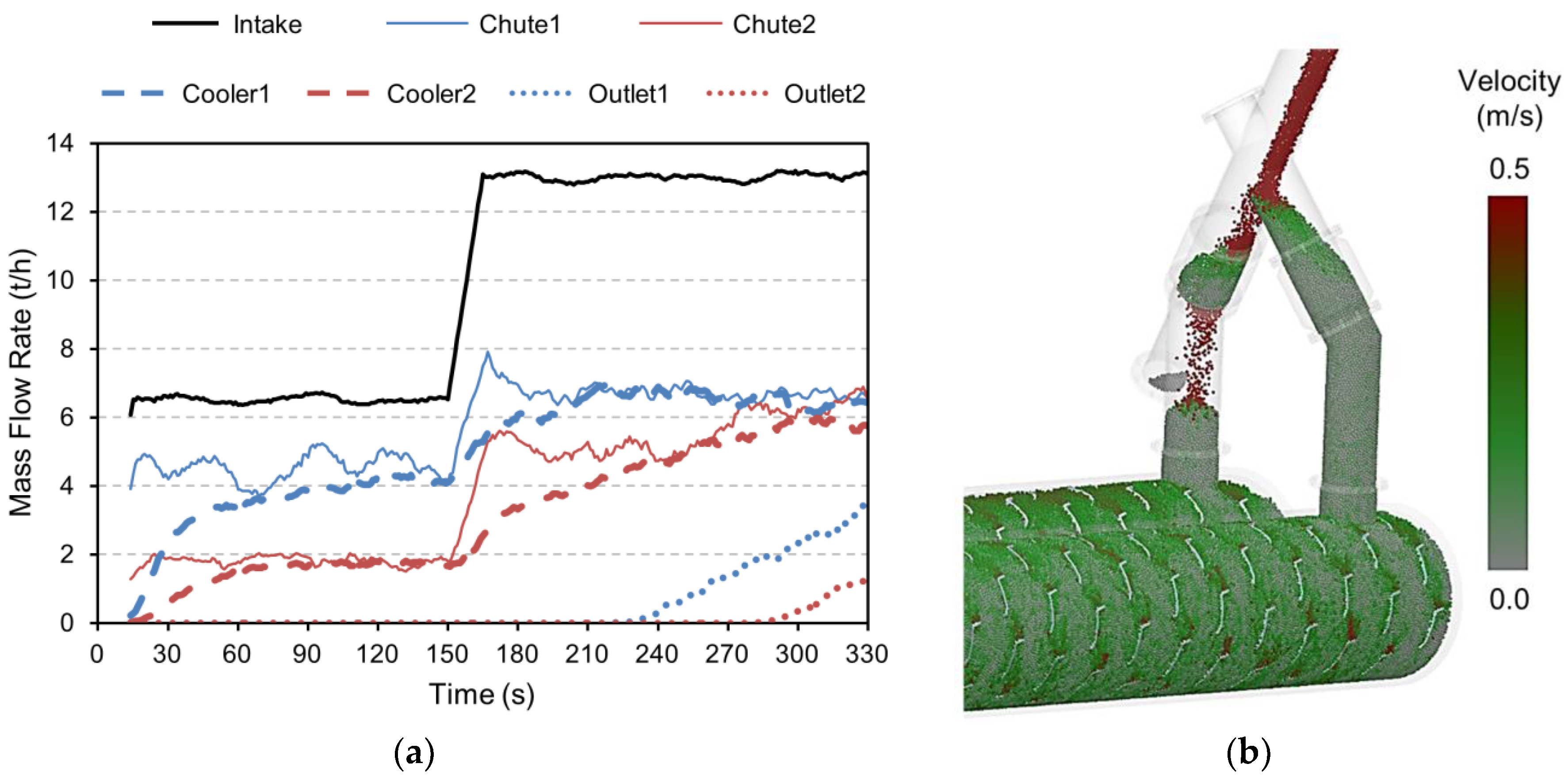
4.1. Analysis of the Current State of Operation

The basic parameter of each conveying device is its transport capacity, i.e., the volume/mass of the material per unit of time. The material flow values obtained from all seven sensors (Figure 3) are shown in Figure 4a. In the first stage of the study, a material flow simulation was performed in the existing facility. This helped create a reference simulation that shows the behavior of the material throughout the system. Figure 4 shows that at the generated mass flow rate of 6.5 t/h, the material fails to separate equally. Instead, 4.6 t/h was fed to the cooler 1 and 1.9 t/h to the cooler 2. The inclination of the 5° of the coolers clearly causes the accumulation of material in their rear part. Cooler 1 operates at the maximum level when the total flow rate is 6.5 t/h. In time T = 150 s, the volume of material generated in the feed pipeline was increased to 13 t/h, resulting in the immediate overloading of cooler 1. After the whole volume of the chute 1 is filled with the material, cooler 2 after a certain period of time, is overloaded as well. In time, T = 330 s, both coolers already operate at their maximum transport capacity of about 6 t/h. Based on the simulation of the process, it is obvious that the inclination of the coolers to some extent negates the paddle pitch on the cooler shafts. The purpose of these paddles is to move the material inside the cooler in the direction of transport and to mix and spread the material over the cooler body. When monitoring a few selected particles entering the cooler from the chute, their movement, time they remained in the cooler, and number of contacts with the cooling shell were analyzed. The average particle speed in the transport direction was 0.02 m∙s⁻¹, which at the cooler length of 6 m means the average time spent in the cooler (cooling time) was 300 s. Analysis of transport and particle movement at the current state of the fly ash cooler system revealed problems in both the chute, which dispense the material between both coolers unevenly and in the conveying capacity of the coolers. The overloading of both coolers is shown in Figure 4b. The transport capacity limit of the existing equipment and the inlet drain was determined (Figure 4a).

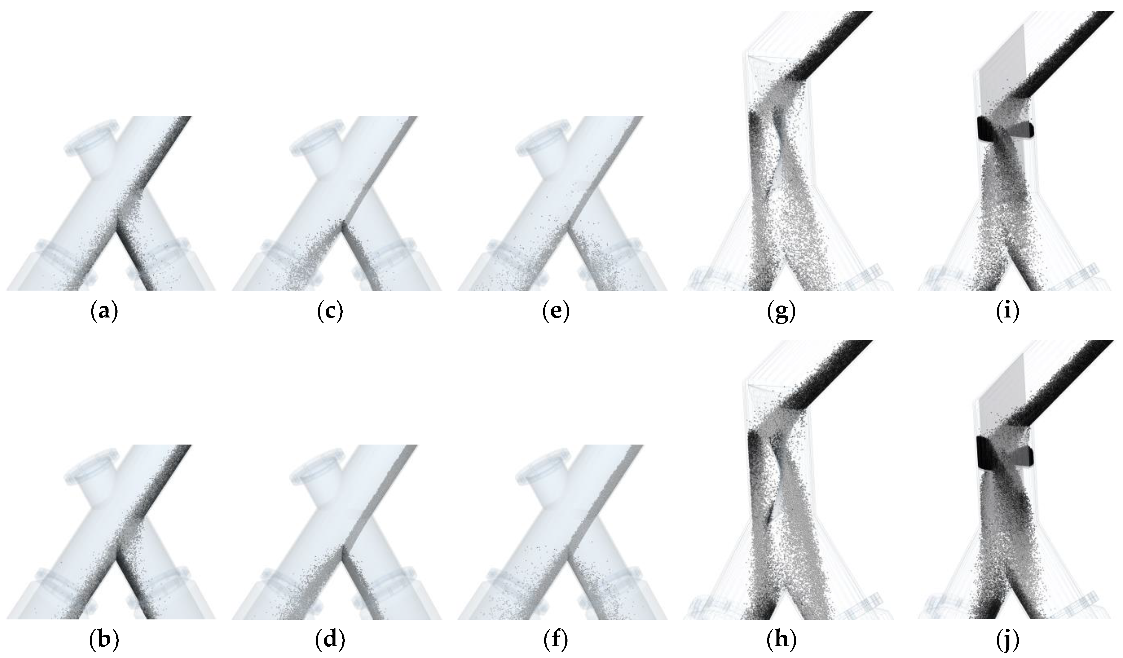
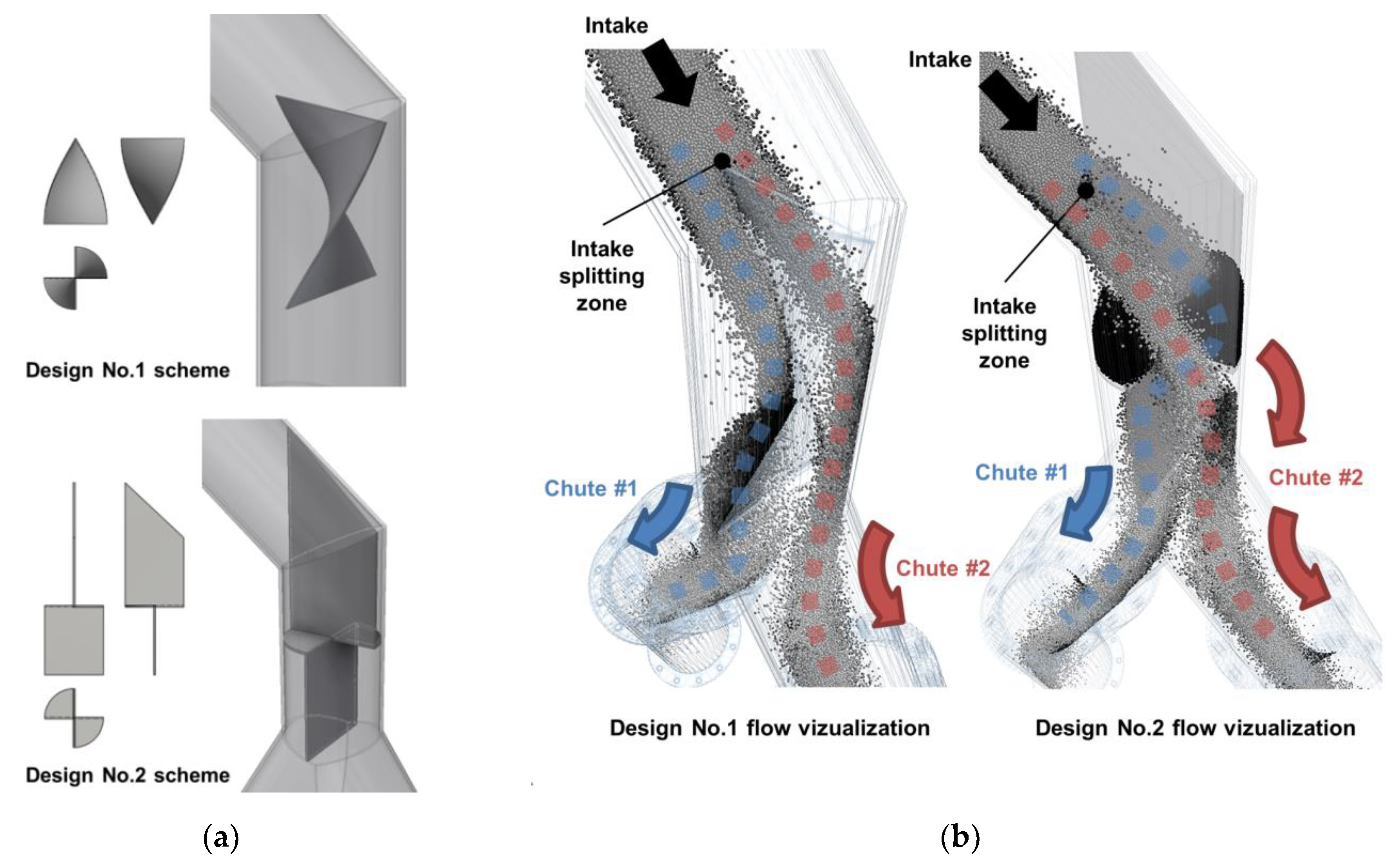
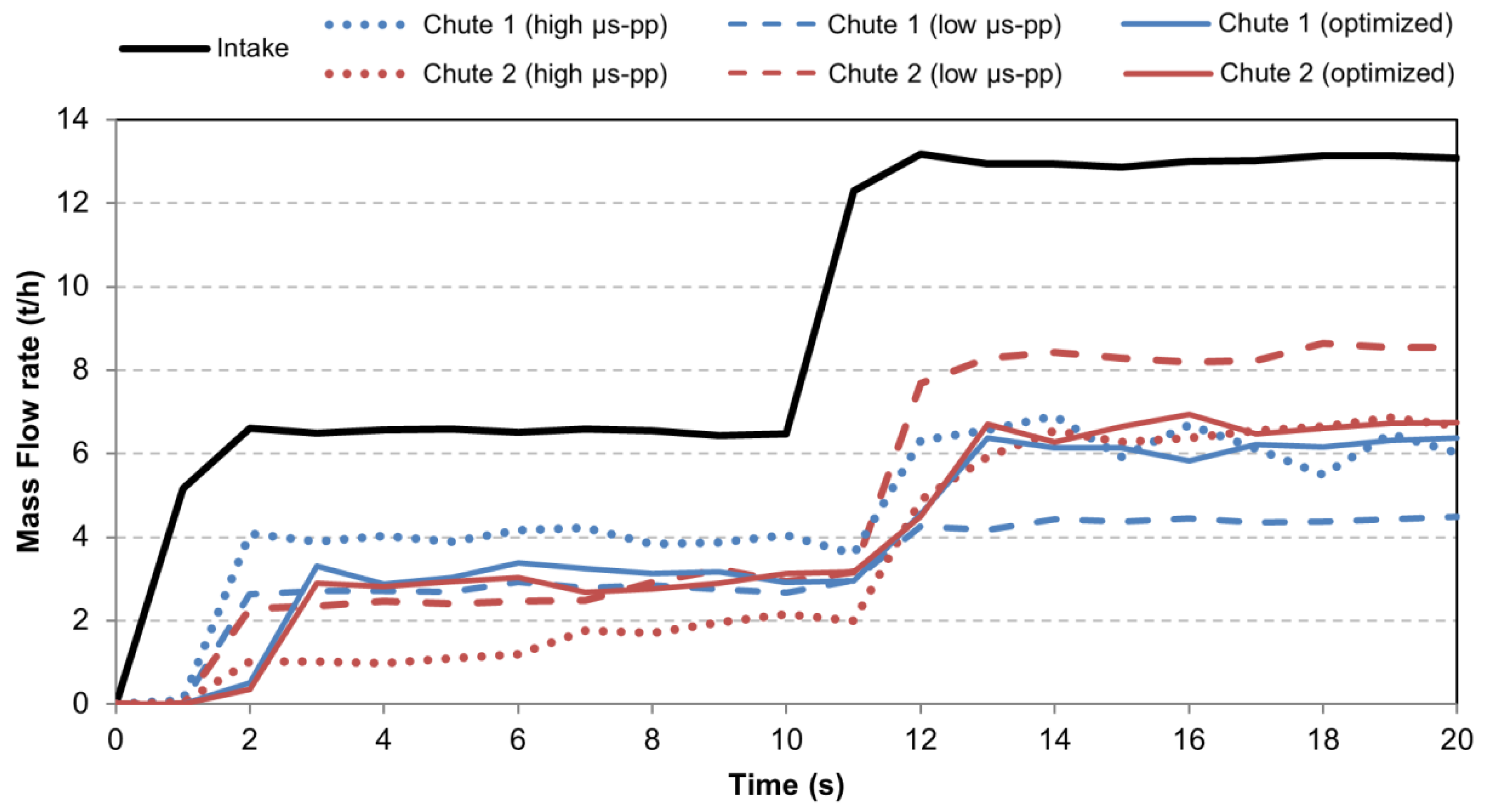
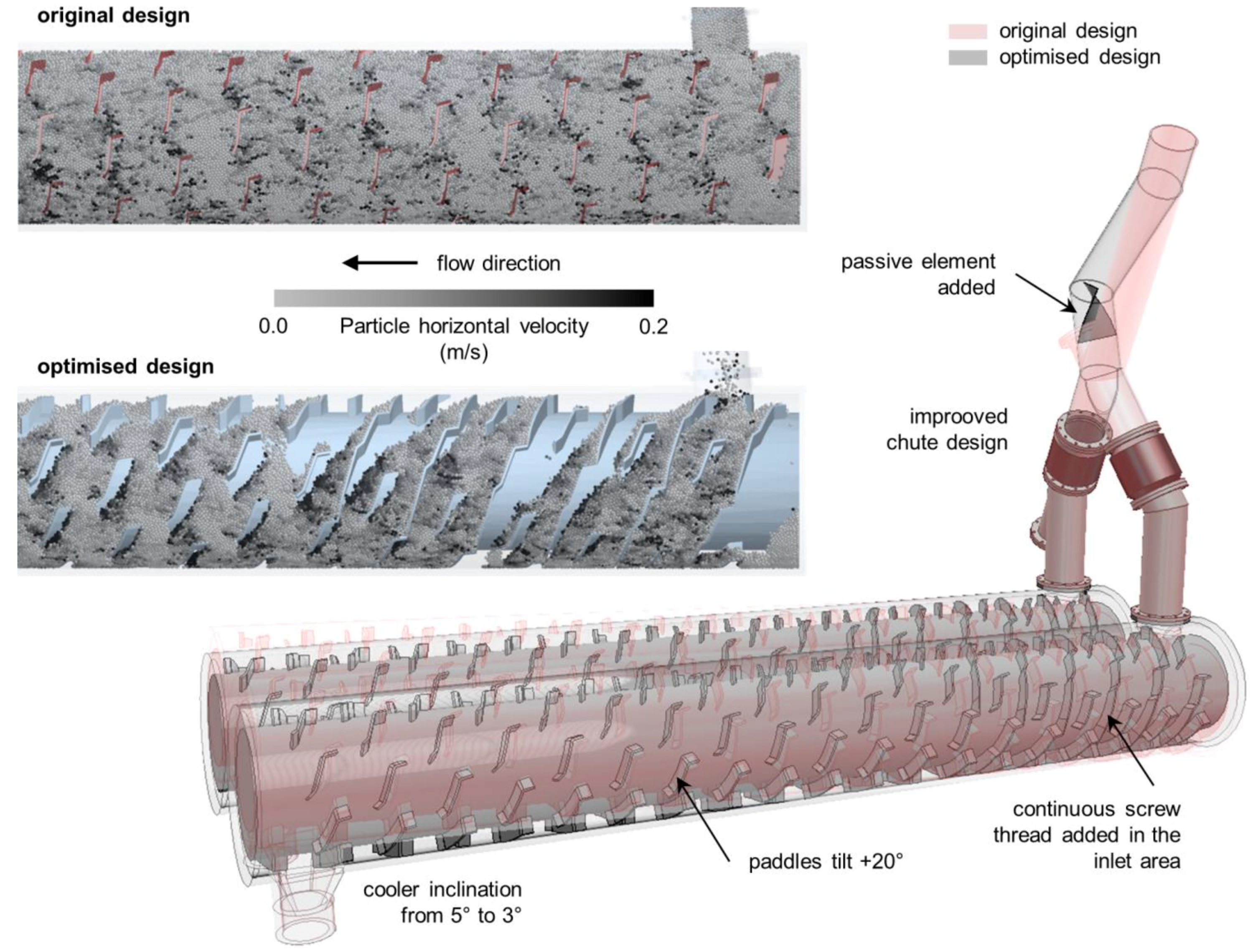
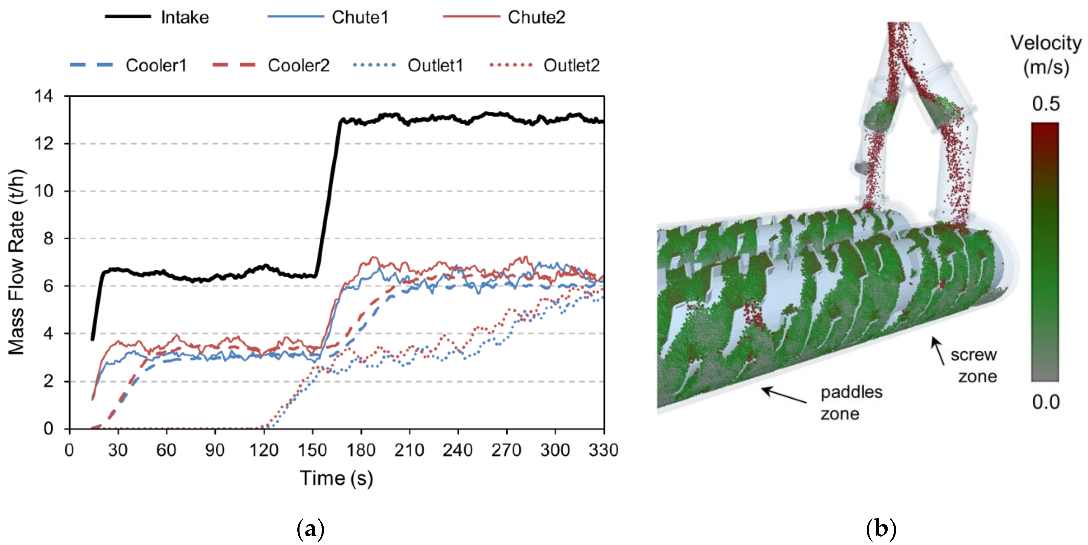
4.2. Inlet Pipeline Design Optimization

In the first phase of the optimization process of the entire system, it was necessary to design adjustments in the chute, to achieve the most uniform distribution of material between the two coolers in all circumstances. At the same time, the positions and inclinations of the inlet and outlet pipes should be respected. This section presents an analysis of the current state of the chute which does not fulfill the required function, which is to equally distribute the input materials into individual coolers. Given the current design of the chute, the volume and rate in which the material is fed into the chute are the most important factors. For the study of the division of the material in the chute, the chute was removed from the overall assembly. The “intake”, “chute 1” and “chute 2” virtual sensors were used to monitor the process of distribution of the input material into both outputs.

A series of 6 simulations was created (Figure 5a–f), where the behavior of the material in the chute was monitored under the various conditions that may occur during operation. The aim was to design such construction modifications that would ensure an optimal distribution of the feed material under all conditions. In these simulations with a total length of T = 20 s, the pipeline was fed at the rate of 6.5 t/h in the first half of the simulation and the rate of 13 t/h in the second half of the simulation, representing the range in which the entire cooling system should work reliably. Three simulations were created for the existing construction of the chute using three different coefficients of particle-particle static friction. The purpose of the different ratios of friction coefficients was to simulate different degrees of aeration of the conveyed material coming from the fluidized bed boiler. This is reflected in material flowability, material velocity in pipelines, etc. In the first simulation of the aerated material, the coefficient of static friction between the particles μ_s-pp was much smaller than the coefficient of static friction between the particles and the contact material μ_s-pw. In the second simulation, the coefficient μ_s-pp = μ_s-pw, whereas in the third simulation μ_s-pp >> μ_s-pw. The behavior of the material under these three different boundary conditions is shown in Figure 5. Figure 5g–j also shows the modified chutes which are not prone to friction ratios of materials and ensures an even distribution of material into both coolers under all operating conditions.

The analysis of the chute proved that its current design is sensitive to the state (aeration/consolidation) of material, the volume of material, and the material velocity, etc. For these reasons, the design of a diverter was proposed to mitigate the above-mentioned issues related to uneven material distribution inside the chute. This solution consists in placing a passive element in the vertical part of the pipeline. Two variants of these passive elements are shown in Figure 6a. Both of these variants gave very similar results of the material distribution in the chute. The principle of their function is the horizontal division of the supply pipeline into two halves. Each of these halves is then passed through a passive element to a part of the chute (chute 1, chute 2) and then to both of the coolers. Figure 6b shows the principle of the distribution and feeding of the material in the chute.

Figure 7 illustrates the flow rate of the material in the chute as determined by “intake,” “chute 1” and “chute 2” virtual sensors (Figure 3). Flow rates for low coefficient μ_s-pp, high coefficient μ_s-pp, and the optimized chute are shown. From the results (Figure 7), it is clear that the original design worked well for just one of the operating modes, either for 6.5 or 13 t/h. While the material with a low coefficient of static friction between the particles fed at the rate of 6.5 t/h was distributed in a fairly satisfactory manner, the rate of 13 t/h was completely inadequate (4.5 t/h to cooler 1 and 8.5 t/h to cooler 2). For material with high coefficient μ_s-pp the opposite situation was observed. This allowed for a transport capacity of 13 t/h but at a dosage of 6.5 t/h, approximately 4.25 t/h was fed to the cooler 1 and 2.25 t/h to the cooler 2. After the modifications, the chute met the function requirements for both the operating conditions and all the properties of the particulate material. This fact makes the solution very versatile with a wide range of applications.

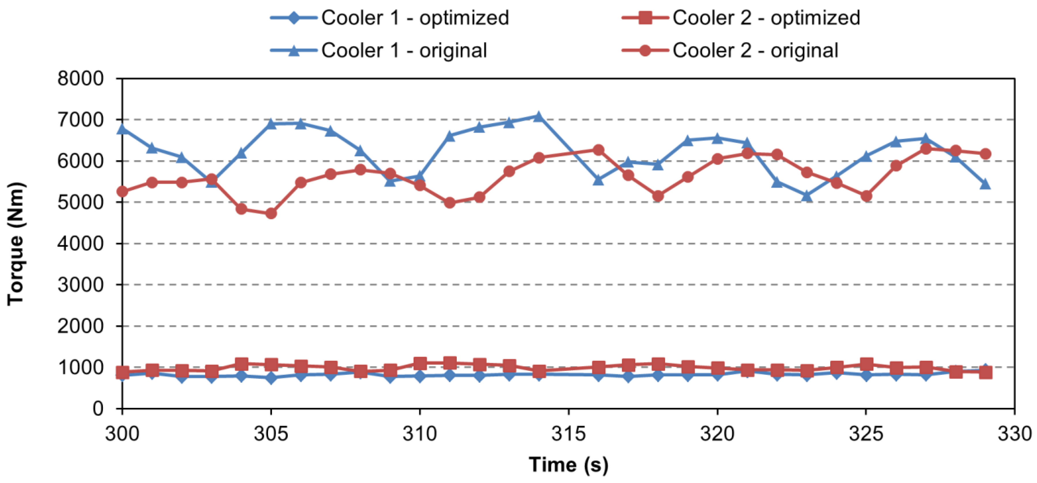
4.3. Rotary Coolers Design Optimization

The second phase of the optimization process of the entire cooling system was to ensure transport and cooling performance. This study focuses primarily on the transport performance and the description of material movement inside the cooler. The analysis of the current state outlined in Section 4.1 shows that the current design of the coolers reaches its limit of functionality in terms of transport capacity. Moreover, in combination with the inappropriate geometry of the chute, overloading of the coolers takes place. The aim is, therefore, to modify the geometry of the coolers to increase the conveying performance of the equipment, while prolonging the time the material stays in the cooler to ensure sufficient cooling efficiency. Based on the existing state, the following two phenomena were observed: (1) the inclination of the paddles located on the cooler shaft is partially negated by the slope of the entire cooler, which slows down the movement of the material in the direction of transport; (2) the material tends to accumulate in the inlet area, thereby blocking the input material and congesting the inlet pipe in the chute. For these reasons, design modifications were made not only to the chute but also to the coolers themselves. All modifications are described and illustrated in Figure 8. Specifically, this included geometrical modification of the chute and addition of a passive element, the installation of several screw threads at the inlet section, the change of the paddle inclination in addition to the reduction of the coolers’ inclination. The process of optimization was primarily based on the visualization of material movement and the experience of operating the coolers. Particle motion in the simulation was used to design modifications. Thanks to this visualization, the designer can make an imagination of how the material flows into the intake pipeline, and he can design suitable passive elements inside the pipeline. The design of small pockets instead of blades on the rotating shaft was considered for the cooler. However, the authoring team feared that this solution would increase energy consumption without significant impact on transport capacity. For this reason, just the blades inclination has been changed. The first simulation of modified coolers showed perfect results, so no other changes had been required. It was found that the changes fulfills the compromise between the mass flow rate and the time of stay of material inside the coolers.

Figure 8 shows a comparison of the material distribution in the cooler at a transport rate of 13 t/h. The color scale of the particles distinguishes the speed in the direction of transport, i.e., in the cooler axis. The optimized cooling system was tested by the same procedure described in Section 4.1, as the original set. Both extremes states in terms of feeding volume were tested once again. Until the time T = 150 s, the system was fed at the rate of 6.5 t/h, and 13 t/h afterward. Figure 9a shows the course of transport performance as determined by the individual virtual sensors. By looking at Figure 9a, it is clear that more balanced and smoother curves of the two coolers were achieved compared to the original state (Figure 4a). It is obvious, that the chute distributes the fed material evenly between the two coolers, ensuring a balanced transport and cooling performance. Several screw threads, located under the inlet pipe, accelerate the speed of the material, preventing its accumulation at the inlet. The conveying capacity was further improved using optimized shape and inclination of the paddles, which gradually move the material in the direction of transport. The material flow through the cooler is also facilitated by the screw feeder that continuously feeds the new material into the cooler. This eliminates the possibility of congestion of the cooler (if the screw conveyor is not overloaded itself) and the material is spread in the interior according to the transport capacity needs. The average particle speed in the transport direction at the rate of 6.5 t/h was 60 mm/s at the screw conveyor part of the cooler and 36 mm/s at the rotary paddles part of the cooler (Figure 8). For a transport capacity of 13 t/h, the average particle speed in the transport direction was 45 mm/s at the screw conveyor part of the cooler and 39 mm/s at the rotary paddles part of the cooler. This corresponds with the average cooling time of the particle in the cooler of about 150 s for both transport capacities. However, at lower flow rates the material is more spread and mixed, which improves the efficiency of the cooling process. The time material stays in the cooler was shorter compared to the original state, which could lead to a high temperature of fly ash at the maximum conveying capacity. In this case, it would be necessary to proceed to more extensive structural modifications, e.g., to extend the coolers, to increase the heat exchange surface, to increase the diameter of the cooler, etc.

At the final stage of the optimization process, torques on both coolers were obtained from simulations data for original coolers as well as the optimized ones. The values of torques are shown in Figure 10. There are data presented for the last 30 seconds of the process. It means the fully loaded coolers at a mass flow rate of approx. 6.5 tonnes per hour in each of them was optimal. The paddles inclination change had a huge effect on the power consumption decreasing while increasing the transport capacity of coolers. In addition, the running of coolers is much more even. All of these fact have another positive effect in costs of the cooling system in power units and consumption savings. All of the values of torques are based on the same DEM input parameters and boundary conditions. Only the geometry of the inlet pipeline and active parts of coolers had been changed.

5. Conclusions

This study presents the possibilities of using DEM modeling in the optimization of chutes and rotary coolers used in fly ash cooling technology at industrial scale. Using this method, it is possible to obtain important data that can be used both in designing new solutions and optimizing existing ones. The method also offers a detailed look into the processes that would not be possible in practice and provides a deeper understanding of the behavior of particulate solids during transportation and processing. It can be very challenging for some companies, to design the correct pipeline for their equipment. The impact of correct design on a whole handling or transport system is presented in this study as well as the solution of the problems by the passive elements inside the pipeline. It can improve the efficiency of the system with very low costs. Bian et al. (2017) [38] published a study of a tumbling ball mill with lifter height optimization which has an effect on torque decreasing it at the final stage.

The analysis of the existing state of cooling technology revealed shortcomings in both the design of the chute and the coolers. The material was unevenly dispensed between the two coolers, which combined with the limited transport capacity of the coolers, led to overflowing and congestion of the whole system. Therefore, after visualization of the material flow using DEM, design measures were proposed to remove these unwanted phenomena. The chute was modified introducing a passive element inside, which greatly improved the flow achieving an equal distribution of the material between both coolers. In addition, the shaft, as well as the rotary paddles, were equipped with a number of screw threads at the inlet to facilitate the movement of the material and to prevent its accumulation. Moreover, the inclination of the entire cooler and paddles were optimized to achieve the required transport capacity with the least cooling time.

Thanks to presented geometric optimization, the energy efficiency of the process has been improved by 80% in power consumption. The torque needed to rotate each of two shafts went down from 6 to 1 kNm. The improved paddles inclination led to significant reduction in resistive forces from material spreading inside the cooler. The geometric optimization of chute increased the working capacity of cooler 1 by 44% from 4.5 to 6.5 t/h. Therefore, the cooler 2 works adequately to cooler 1 which is no longer overloading. For a transport capacity of 13 t/h, an average cooling time of the fly ash of about 150 s was achieved. The cooling time is shorter compared to the original state, which could lead to a high temperature of outputting fly ash at the maximum conveying capacity. In this case, it would be necessary to proceed to more extensive structural modifications.

In general, DEM represents a truly innovative approach for the design of equipment where particulate solids are present. Above all, combined with or without other numerical models, it can become an everyday tool for designers in the future. It can be used not only in the initial design phase, in the conception of the design, but also when the equipment is already designed, and reverse engineering is then needed after diagnosing malfunction. The results obtained contribute to increasing the operational efficiency and competitiveness of the equipment analyzed. Similar case studies can be very inviting not just for academics, but also for many companies which are focused on particulates handling and processing encouraging them to join the DEM community and save on costs from solving different issues.

References

1. Wait, R. Discrete element models of particle flows. Math Model Anal. 2001, 6, 156–164. [Google Scholar] [CrossRef]
2. Cleary, P.W. Discrete element modelling of industrial granular flow applications. Task. q.-Sci. Bull. 1998, 2, 385–416. [Google Scholar]
3. Antonyuk, S.; Palis, S.; Heinrich, S. Breakage behaviour of agglomerates and crystals by static loading and impact. Powder Technol. 2011, 206, 88–98. [Google Scholar] [CrossRef]
4. Owen, P.J.; Cleary, P.W. Prediction of screw conveyor performance using the Discrete Element Method (DEM). Powder Technol. 2009, 193, 274–288. [Google Scholar] [CrossRef]
5. Feda, J. Mechanics of Particulate Materials—The Principles, 2nd ed.; Academia Prague: Prague, Czech Republic, 1982; ISBN 0-444-99712-X. [Google Scholar]
6. Hendrik, O.; Kerst, K.; Roloff, C.; Janiga, G.; Katterfeld, A. CFD-DEM simulation and experimental investigation of the flow behavior of lunar regolith JSC-1A. Particuology 2018, in press. [Google Scholar] [CrossRef]
7. Forsström, D.; Pär, J. Calibration and validation of a large scale abrasive wear model by coupling DEM-FEM: Local failure prediction from abrasive wear of tipper bodies during unloading of granular material. Eng. Fail. Anal. 2016, 66, 274–283. [Google Scholar] [CrossRef]
8. Barrios, G.K.; Tavares, L.M. A preliminary model of high pressure roll grinding using the discrete element method and multi-body dynamics coupling. Int. J. Miner. Process. 2016, 156, 32–42. [Google Scholar] [CrossRef]
9. Fedorko, G.; Ivančo, V. Analysis of Force Ratios in Conveyor Belt of Classic Belt Conveyor. Procedia. Eng. 2012, 48, 123–128. [Google Scholar] [CrossRef]
10. Manjula, E.V.P.J.; Ariyaratne, W.K.H.; Ratnayake, C.; Melaaen, M.C. A review of CFD modelling studies on pneumatic conveying and challenges in modelling offshore drill cuttings transport. Powder Technol. 2017, 305, 782–793. [Google Scholar] [CrossRef]
11. Chen, W.; Roberts, A.; Katterfeld, A.; Wheeler, C. Modelling the stability of iron ore bulk cargoes during marine transport. Powder Technol. 2018, 326, 255–264. [Google Scholar] [CrossRef]
12. Markauskas, D.; Ramírez-Gómez, Á.; Kačianauskas, R.; Zdancevičius, E. Maize grain shape approaches for DEM modelling. Comput. Electron. Agric. 2015, 118, 247–258. [Google Scholar] [CrossRef]
13. Bai, Y.; He, F. Modeling on the Effect of Coal Loads on kinetic Energy of Balls for Ball Mills. Energies 2015, 8, 6859–6880. [Google Scholar] [CrossRef]
14. Cundall, P.A.; Strack, O.D.L. A discrete numerical model for granular assemblies. Geotech. 1979, 29, 47–65. [Google Scholar] [CrossRef]
15. Marigo, M. Discrete Element Method Modelling of Complex Granular Motion in Mixing Vessels: Evaluation and Validation. Ph.D. Thesis, The University of Birmingham, Birmingham, UK, 2012. [Google Scholar]
16. Kannan, A.S.; Jareteg, K.; Lassen, N.C.K.; Carstensen, J.M.; Hansen, M.A.E.; Dam, F. Design and performance optimization of gravity tables using a combined CFD-DEM framework. Powder Technol. 2017, 318, 423–440. [Google Scholar] [CrossRef]
17. Haeri, S. Optimisation of paddle type spreaders for powder bed preparation in Additive Manufacturing using DEM simulations. Powder Technol. 2017, 321, 94–104. [Google Scholar] [CrossRef]
18. Zhao, L.; Zhao, Y.; Bao, C.; Hou, Q.; Yu, A. Optimisation of a circularly vibrating screen based on DEM simulation and Taguchi orthogonal experimental design. Powder Technol. 2017, 310, 307–317. [Google Scholar] [CrossRef]
19. Pantaleev, S.; Yordanova, S.; Janda, A.; Marigo, M.; Ooi, J.Y. An experimentally validated DEM study of powder mixing in a paddle paddle mixer. Powder Technol. 2017, 311, 287–302. [Google Scholar] [CrossRef]
20. Wang, D.; Servin, M.; Mickelsson, K.O. Outlet design optimization based on large-scale nonsmooth DEM simulation. Powder Technol. 2014, 253, 438–443. [Google Scholar] [CrossRef] [Green Version]
21. Kulka, J.; Mantic, M.; Faltinova, E.; Molnar, V.; Fedorko, G. Failure analysis of the foundry crane to increase its working parameters. Eng. Fail. Anal. 2018, 88, 25–34. [Google Scholar] [CrossRef]
22. Roberts, A.W.; Wensrich, C.M. Flow dynamics or ‘quaking’in gravity discharge from silos. Chem. Eng. Sci. 2002, 57, 295–305. [Google Scholar] [CrossRef]
23. Klinzing, G.E. A review of pneumatic conveying status, advances and projections. Powder Technol. 2018, 333, 78–90. [Google Scholar] [CrossRef]
24. Nečas, J.; Hlosta, J.; Žurovec, D.; Žídek, M.; Rozbroj, J.; Zegzulka, J. Feeder Type Optimisation for the Plain Flow Discharge Process of an Underground Hopper by Discrete Element Modelling. Adv. Sci. Technol. Res. J. 2017, 11, 246–252. [Google Scholar] [CrossRef] [Green Version]
25. Roberts, A.W. Particle Technology—Reflections and Horizons. Chem. Eng. Res. Des. 1998, 76, 775–796. [Google Scholar] [CrossRef]
26. Drescher, A.; Josselin, G. Photoelastic verification of a mechanical model for the flow of a granular material. J. Mech. Phys. Solids. 1972, 20, 337–340. [Google Scholar] [CrossRef]
27. Raclavská, H.; Corsaro, A.; Juchelková, D.; Sassmanová, V.; Frantík, J. Effect of temperature on the enrichment and volatility of 18 elements during pyrolysis of biomass, coal, and tires. Fuel Process. Technol. 2015, 131, 330–337. [Google Scholar] [CrossRef]
28. Belohlav, Z.; Brenková, L.; Hanika, J.; Durdil, P.; Rapek, P.; Tomasek, V. Effect of Drug Active Substance Particles on Wet Granulation Process. Chem. Eng. Res. Des. 2017, 85, 974–980. [Google Scholar] [CrossRef]
29. Hlosta, J.; Zurovec, D.; Gelnar, D.; Zegzulka, J.; Necas, J. Thermal Conductivity Measurement of Bulk Solids. Chem. Eng. Technol. 2017, 40, 1876–1884. [Google Scholar] [CrossRef]
30. Baniasadi, M.; Baniasadi, M.; Peters, B. Coupled CFD-DEM with heat and mass transfer to investigate the melting of a granular packed bed. Chem. Eng. Sci. 2018, 178, 136–145. [Google Scholar] [CrossRef]
31. Bellan, S.; Matsubara, K.; Cho, H.S.; Gokon, N.; Kodama, T. A CFD-DEM study of hydrodynamics with heat transfer in a gas-solid fluidized bed reactor for solar thermal applications. Int. J. Heat Mass Transf. 2018, 116, 377–392. [Google Scholar] [CrossRef]
32. Wu, H.; Gui, N.; Yang, X.; Tu, J.; Jiang, S. A smoothed void fraction method for CFD-DEM simulation of packed pebble beds with particle thermal radiation. Int. J. Heat Mass Transf. 2018, 118, 275–288. [Google Scholar] [CrossRef]
33. Tsuji, Y.; Tanaka, T.; Ishida, T. Lagrangian numerical simulation of plug flow of cohesionless particles in a horizontal pipe. Powder Technol. 1992, 71, 239–250. [Google Scholar] [CrossRef]
34. Raymus, G.J. Handling of Bulk Solids. In Chemical Engineers’ Handbook, 6th ed.; Perry, R.H., Green, D., Eds.; McGraw-Hill: New York, NY, USA, 1985; ISBN 978-0070494794. [Google Scholar]
35. Schwartz, S.R.; Richardson, D.C.; Michel, P. An implementation of the soft-sphere discrete element method in a high-performance parallel gravity tree-code. Granul. Matter 2012, 14, 363–380. [Google Scholar] [CrossRef]
36. Hlosta, J.; Zurovec, D.; Rozbroj, J.; Ramírez-Gómez, Á.; Necas, J.; Zegzulka, J. Experimental determination of particle-particle restitution coefficient via double pendulum method. Chem. Eng. Res. Des. 2018, in press. [Google Scholar] [CrossRef]
37. Beakawi Al-Hashemi, H.M.; Baghabra Al-Amoudi, O.S. A review on the angle of repose of granular materials. Powder Technol. 2018, 330, 397–417. [Google Scholar] [CrossRef]
38. Bian, X.; Wang, G.; Wang, H.; Wang, S.; Lv, W. Effect of lifters and mill speed on particle behaviour, torque, and power consumption of a tumbling ball mill: Experimental study and DEM simulation. Miner. Eng. 2017, 105, 22–35. [Google Scholar] [CrossRef]
Figure 1. General principle of discrete element method (DEM) modeling of every single process simulation.
Energies 11 01849 g001
Figure 2. Computer-aided design (CAD) data assembly with all active geometries which have been used for the discrete element method (DEM) simulation.
Energies 11 01849 g002
Figure 3. Imported 3D CAD model and virtual sensors placing.
Energies 11 01849 g003
Figure 4. (a) Mass flow rates results data obtained from different sensors; (b) Overloading of coolers and inlet pipeline blockage.
Energies 11 01849 g004
Figure 5. (a) Original design, low μs-pp, 6.5 t/h; (b) Original design, low μs-pp, 13 t/h; (c) Original design, medium μs-pp, 6.5 t/h; (d) Original design, medium μs-pp, 13 t/h; (e) Original design, high μs-pp, 6.5 t/h; (f) Original design, high μs-pp, 13 t/h; (g) Optimized design No.1, medium μs-pp, 6.5 t/h; (h) Optimized design No.1, medium μs-pp, 13 t/h; (i) Optimized design No.2, medium μs-pp, 6.5 t/h; (j) Optimized design No.2, medium μs-pp, 13 t/h.
Energies 11 01849 g005
Figure 6. Inlet pipeline chute optimized design: (a) two variants of passive elements; (b) material flow visualization.
Energies 11 01849 g006
Figure 7. Mass flow rates results data obtained from inlet pipe and chutes sensors.
Energies 11 01849 g007
Figure 8. Original and optimized rotary coolers design comparison; list of upgrades.
Energies 11 01849 g008
Figure 9. (a) Mass flow rates results data obtained from different sensors; (b) Optimised coolers.
Energies 11 01849 g009
Figure 10. Torques on shafts of original and optimized coolers at maximal transport capacity.
Energies 11 01849 g010