Article

Non-Distorted Optimization Spectrum Analysis

1
Department of Electrical Engineering, I-Shou University, Kaohsiung 840, Taiwan
2
Center of Teaching and Research, Kaohsiung Municipal Ta-Tung Hospital, Kaohsiung Medical University Hospital, Kaohsiung Medical University, Kaohsiung 807, Taiwan
*
Author to whom correspondence should be addressed.
Energies 2018, 11(7), 1841; https://doi.org/10.3390/en11071841
Submission received: 8 June 2018 / Revised: 9 July 2018 / Accepted: 10 July 2018 / Published: 13 July 2018

Abstract

:
The discrete Fourier transform is extensively applied in spectrum analysis. However, the sampled signal is random, and the discrete Fourier transform has its own specific limitations. Thus, errors will inevitably occur in time–frequency transformation work. The most common are the leakage effects of the spectrum that are caused from the scale of the spectrum not being able to match the characteristics of the signal. The optimal spectrum is proposed to overcome this defect by adjusting the frequency scale to fit signal characteristics. This includes three stages whereby frequency scale can match signal characteristics. Firstly, the signal parameters must be found. Secondly, the frequency scale can be determined from these signal parameters. Finally, the optimal spectrum can be realized using the adjustable spectrum with the new frequency scale. After processing the optimal spectrum, the leakage effects of the signal will be decreased to a minimum. This method preserves signal characteristics in the optimization process, which reaches the ideal of non-distortion.

1. Introduction

The field of engineering includes electrical engineering [1,2], electronic engineering [3,4,5], mechanical engineering [6,7], civil engineering [8,9], structural engineering [10] and others, where system behavior can often be described by differential equations. The solution to the differential equation includes frequency, damping, amplitude, and phase, and while frequency and damping are the characteristic roots and are not affected by the initial conditions or boundary conditions, the amplitude and phase change due to different conditions. Since the system response is usually periodic, time-frequency conversion is often used in the analysis of these responses to convert a time-domain signal into a frequency-domain signal.
Discrete Fourier transforms (DFTs) are a powerful tool, as they reveal periodicities in input data as well as the relative strengths of any periodic components. Because of the limitations of DFTs, the following conditions must be noted when DFTs are applied:
(1)
The sampling rate must be higher than twice the highest frequency of the signal.
(2)
Although users usually take DFTs to analyze complex exponential signals and observe the frequency response of a system, essentially, DFTs always regard signals as periodic.
As a result of the sampling of a signal being random and DFTs having their specific limitations, when a digital signal is transformed by a DFT the error usually occurs in violation of these conditions. The most frequent error is that the sampling time is not an integer multiple of the signal period, thereby creating a discontinuity in the terminal of the signal in the time domain. Consequently, in the frequency domain, it makes the component frequencies not equal to integer multiples of the frequency resolution. No suitable scale can display accurate values, and values will spread nearby to the closest bins, which causes distortion of both frequencies and amplitudes. This effect is called the “picket fence” or the “leakage effect”, which seriously affects the results of DFTs. The effect causes parameters of periodic signals to not be obtained exactly, sets the bandwidth of periodic components to non-zero values, and creates confusion between periodic and non-periodic components [11].
Considering the leakage effect, many algorithms have been proposed to calculate signal parameters. The group power method provides a simple way to analyze the amplitudes of modes [12,13]. Using the interpolated fast Fourier transform (IFFT) algorithm, all parameters can be obtained accurately [14,15,16,17]. Alternatively, many methods have been developed to solve the leakage effect. The window methods are among the most popular solutions to overcome this effect. A signal can be multiplied by a window function to reduce the discontinuity in the terminal of the signal [18,19]. In the frequency domain, the side lobes will be relatively well eliminated. The zero-padding method expands the sampling period to fit the period of the sampled signal by adding zeros [20]. In the frequency domain, the harmonic frequencies will be located at bin values. The integer periodic extension method reproduces the sampling number to several times that of the original sampling number, which reduces the leakage effect quite handily [21]. However, characteristics of the signal are changed from those in the original by the above-mentioned methods. These methods change the signal characteristics to match the frequency scale. Although the leakage effect on the spectrum is improved, the values on bins are not the real values. The method of spectrum analysis optimization has also been proposed, by changing the scale parameters to reach the optimal analysis [22]. Nevertheless, a step of digital signal sampling is used in this method, and a slight error will show accordingly in the result.
In this paper we propose the method of optimal spectrum analysis. This method not only restrains the leakage effect on the spectrum, but also avoids the error of re-sampling to preserve signal characteristics. In this paper we adjust the frequency scale to match signal characteristics so that they are preserved. This process includes three stages: Parameter estimation, optimal scale parameter selection, and adjustable spectrum.
In the parameter estimation process, this paper regards components of a signal as being not only periodic but also possibly complex exponential, which can conform to most behaviors of physical systems. The complex exponential parameters include frequency, damping, amplitude, and phase. If the damping is equal to zero, the component is periodic. Parameter estimation is aimed at calculating parameters of each component, which provides the reference for frequency scale adjustment.
Optimal scale parameter selection determines the two parameters of sampling number and scale shift. The matching degree of signal characteristics and frequency scale can be expressed by the leakage energy. The leakage energy is established as a function of sampling number, scale shift, and component parameters. Because the component parameters are fixed, the leakage energy will be varied to follow the sampling number and scale shift. When these two parameters decrease the leakage energy to the global minimum, their frequency scale will have the optimal analysis result for the signal.
In the adjustable spectrum, the frequency scale is decided by the sampling number and scale shift. The variation in the sampling number can be achieved by increasing or decreasing the sampling number, and additionally, the scale shift can be accomplished by multiplying the signal with a shift function. This step can change not only the frequency scale, but also preserve signal characteristics.
This method optimizes the result near to the original scale, where the leakage effect is eliminated under very fine tuning, and the result is insensitive to un-expected errors. Moreover, this method has some advantages: The signal characteristics are preserved in the optimization process, the periodicity and non-periodicity of components can be recognized, and parameters of the periodic component can be directly obtained from the spectrum. In this paper, the theory is also verified by a practical instrument.

2. Theory

This section interprets the theory and the procedure. The theory includes parameter estimation, optimal scale parameter selection, and adjustable spectrum. The procedure integrates the above-mentioned theory as a complete algorithm.

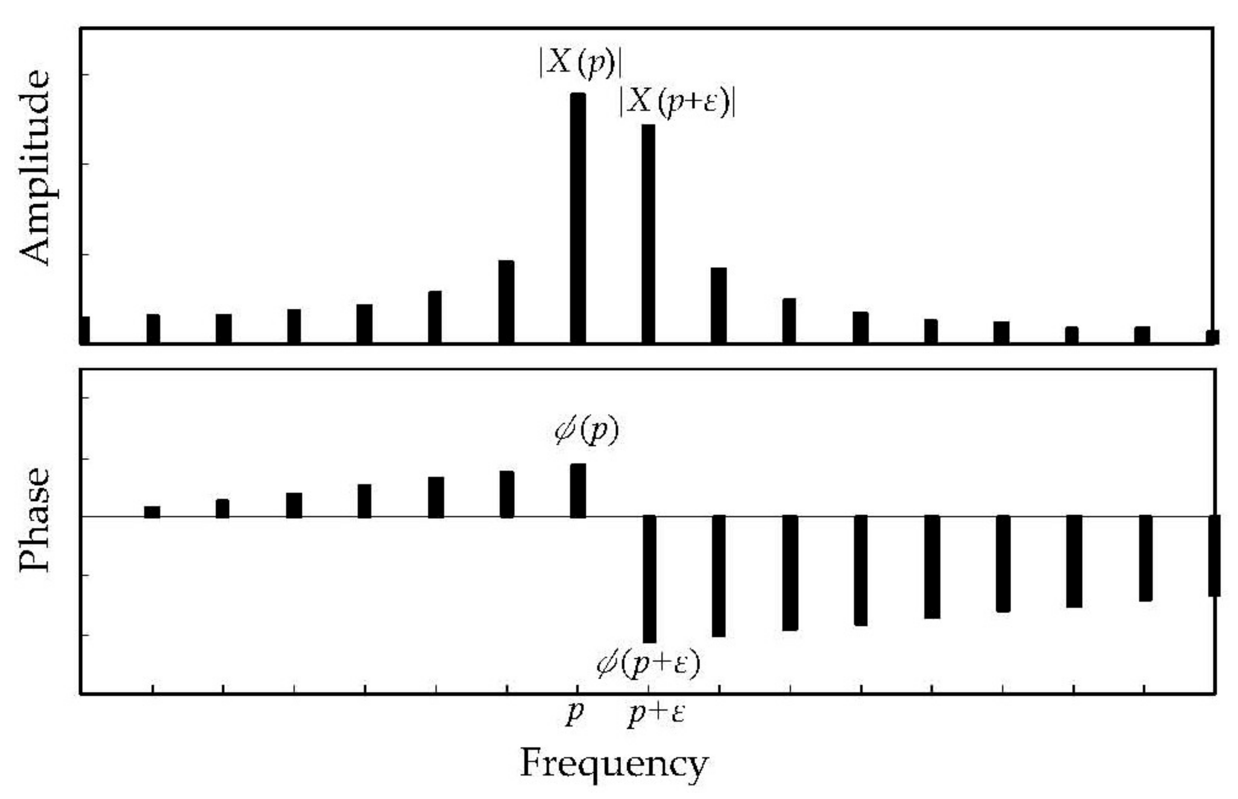
2.1. Parameter Estimation

This section analyzes component parameters by the frequency–domain interpolation algorithm (FDIA) [23]. The signal is regarded as complex exponential in this paper; that is, a signal can be expressed as:
x ( n ) = k = 1 K A k e α k n / N cos ( 2 π f k n N + φ k ) ,   n = 0 , 1 , , N 1
where f is frequency, α is damping, A is amplitude, and φ is phase. After applying the DFT and ignoring the influence from the negative frequency domain, the spectrum can be written as:
X ( m ) = k = 1 K 0.5 A k φ k 1 e α k + j 2 π ( f k m ) 1 e ( α k + j 2 π ( f k m ) ) / N ,   m = 0 , 1 , , N 1
Each component will generate its own band on the spectrum. Using the band data, parameters corresponding to the component can be found. The closer a bin m is to the component frequency fk, the more influence the component has on the value of this bin. This makes the energy spread around the component frequency. Near to the component frequency, the amplitudes are more obvious. Therefore, each component parameter can be found from the bin data with the two highest amplitudes for the corresponding band.
The following illustrates the calculation for a certain component. For a clear description, the symbols used are first shown in Figure 1. Figure 1 is the spectrum corresponding to a complex exponential signal, with the two largest vectors in the band are X(p) and X(p + ε), where ε is equal to 1 or −1, respectively, if |X(p + 1)| ≥ |X(p − 1)| or not. Bins p and p + ε are also used. These four data points are the references for parameter estimation.
The two auxiliary equations are established firstly:
ρ = X ( p + ε ) / X ( p )
and:
z = 1 ρ 1 ρ e j 2 π ε / N
The frequency bias, frequency and the damping can then be found:
δ = N 2 π arg ( z )
f = p + δ
α = 2 π N ln | z |
Once δ and α are determined, the third auxiliary equation can be established:
D = 1 e α + j 2 π δ 1 e ( α + j 2 π δ ) / N
The complex coefficient A φ is easily determined from Equations (9) and (10):
A = | X ( p ) / D |
φ = arg ( X ( p ) / D )
If a component is periodic, its energy will centralize at a certain bin after scale adjustment. However, if the component is non-periodic, its energy will spread nearby to the bin after scale adjustment. Whether the component is periodic or not, for a complex exponential component, the largest amplitude that can influence a bin is:
| X | = NA 2 1 e α α

2.2. Optimal Scale Parameter Selection

The concept of optimal scale parameters involves scale parameters that can be adjusted such that their component frequencies are located as close to bins as possible. This technique can centralize the energy of the periodic component. The concept is also regularly used to optimize the non-periodic component. After eliminating the leakage effect, the non-zero bandwidth of the non-periodic component is purely caused by its damping [24,25].
If the frequency of a periodic component is equal to a bin m, all of the energy will only affect bin m, and not the nearby bins. However, if the frequency cannot be matched with any bin, the leakage effect occurs. This phenomenon can be observed in Figure 2. Figure 1 also shows the results of processing signals with a DFT, and in this figure the leakage effect caused by frequencies cannot be matched with the frequency scale. |X(p)| represents the amplitude of the bin which is nearest to the component frequency. Apart from these amplitudes, the other amplitudes are regarded as leakage energy. If a signal includes K components, according to the concept of group power, the total energy of a signal S2 can be expressed as:
S 2 = 2 k = 1 K | X k ( p ) / N | 2 + 2 L
The leakage energy can represent the degree of the match between component parameters and the frequency scale. The frequency f and the amplitude A can be found in the above section, and the leakage energy can be written as:
L 1 N 2 k = 1 K ( 1 2 | X k | sin π δ k ) 2
Changing the leakage energy can be achieved only by adjusting the frequency scale. The frequency scale is decided by scale parameters (sampling number N’ and scale shift Ss). The sampling number decides the distance between each pair of bins, and scale shift simultaneously varies all bins by a certain value. The influence of these two parameters on the scale is shown in Figure 3. In the original spectrum, N’ is fixed as N and Ss is set to 0. This section regards these two parameters as adjustable, and the relation of the new bin to the original is given by:
m = N ( m + S s ) / N
Owing to the adjusted scale, the frequency bias will be changed. The order of scale parameter adjustment is the sampling number first, and scaling the shift second. After the sampling number has been adjusted, the new frequency bias δ’ becomes:
δ = f mN / N
where the following condition must be satisfied:
| δ | = MIN { | f mN / N | , m = 0 , 1 , , N 1 }
Using scale adjustment, the leakage energy will become:
L 1 N 2 k = 1 K ( 0.5 | X k | sin π ( δ k S s ) N N ) 2
The optimal scale parameters include the optimal sampling number and the optimal scale shift. Under the condition of arbitrarily frequency biases, the scale shift that minimizes the leakage energy is:
S s = ( k = 1 K | X k | 2 δ k ) / ( k = 1 K | X k | 2 )
Because of scale shifting, the leakage energy will decrease to a local minimum, and Equation (17) will become:
L min = ( π N 2 N 2 ) 2 k = 1 K ( | X k | 2 k = 1 K | X k | 2 | δ k δ k | k = 1 K | X k | 2 ) 2
where Lmin is defined as the minimal leakage energy.
Equation (19) is the minimum leakage energy after scale shifting using a certain sampling number. In applications, Equation (19) can be simplified if needed:
L min = k = 1 K k = 1 K | X k | | X k | | δ k δ k |
Because the relation between L’min and the sampling number is non-linear, a specific range must be searched one-by-one to find the minimum, L’min. Once the minimum, L’min, is found, the sampling number under this condition is optimal and the optimal scale shift can be obtained by Equation (18). From the optimal sampling number and optimal scale shift, the optimal frequency scale can be determined.

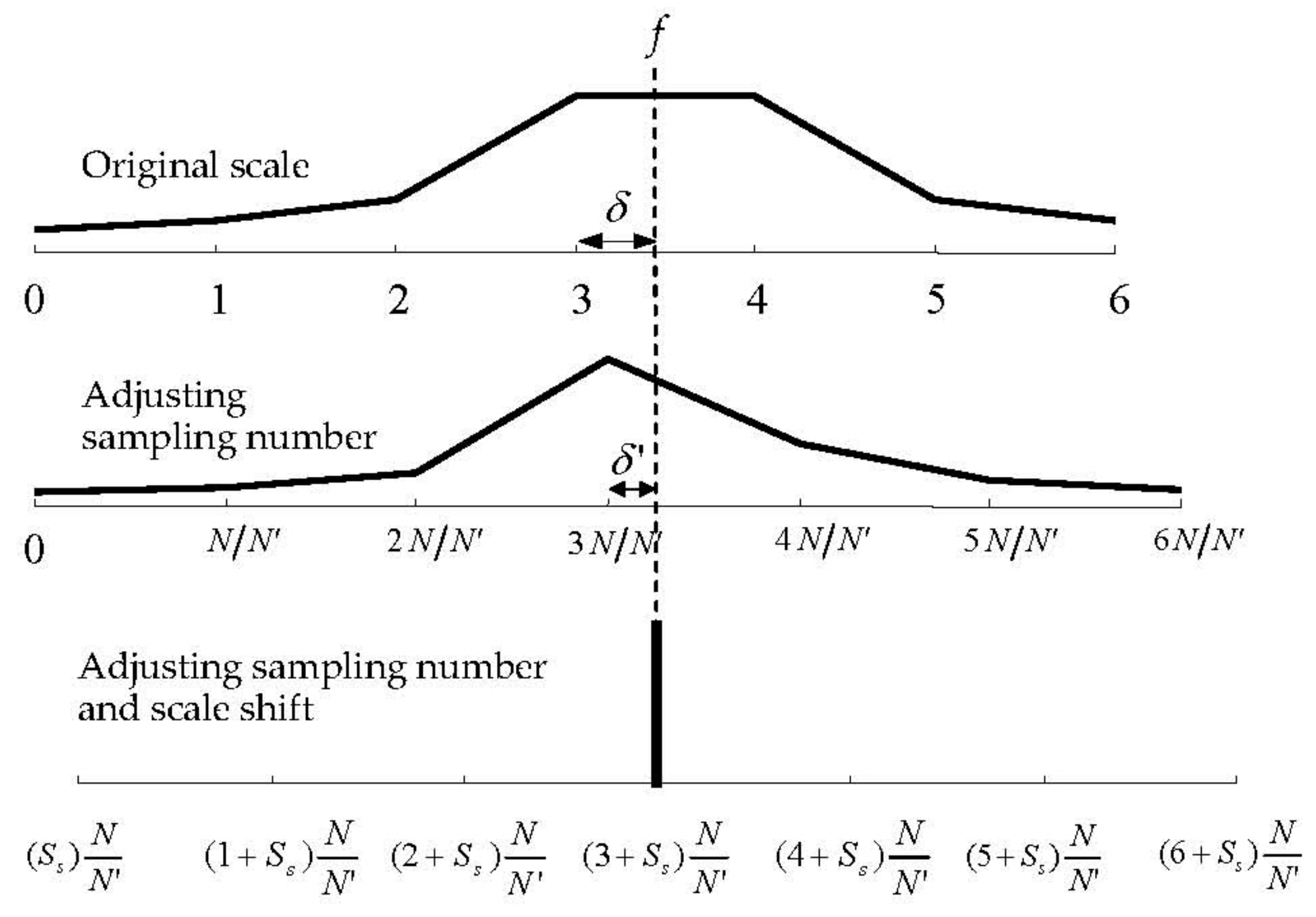
2.3. Adjustable Spectrum

The adjustable spectrum method involves adjusting the frequency scale. To preserving signal characteristics, in this paper we set the frequency scale according to the sampling number N’ and the scale shift Ss. The following explains the theory of adjusting these two parameters.
The sampling number decides the distance between each pair of bins. This distance can be also adjusted by changing the sampling rate [26]. When the sampling rate is changed, the new signal must be obtained by re-sampling via the numerical method. This method will cause either large or small errors, especially for the higher frequency components [27]. In the method of changing the sampling number, the new signal is just the data length variation of the original one, which can completely preserve the signal characteristics.
x ( n ) = x ( n ) ,   n = 0 , 1 , , N 1
According to the frequency-shifting theorem, the shift Ss in the frequency domain is equivalent to multiplying the signal with exp(jSsn/N’) in the time domain. That is, the scale shift can be realized by the following equation:
X ( m ) = n = 0 N 1 x ( n ) exp ( j 2 π n m + S s N ) ,   m = 0 , 1 , , N 1
Equations (21) and (22) are the transform of the adjustable spectrum. In the DFT, N is fixed and Ss is 0, so that the scale cannot flexibly respond for different signal characteristics. These two parameters in the adjustable spectrum can be changed arbitrarily, which scales the frequency in a very flexible way. After scale adjustment, the real frequencies freal corresponding to the bins are:
f real ( m ) = ( m + S s ) R / N ,   m = 0 , 1 , , N 1
As the sampling number is only slightly different from 2r, it can be changed arbitrarily. In this paper we run DFTs based on Equation (22) instead of the fast Fourier transform (FFT).

2.4. Procedure

This section integrates the above-mentioned theory as a complete procedure; each step is explicated as per the following:
Step 1: Signal sampling: Sample an analog signal as a digital one, with sample number N and sampling rate R. In this step, the sampling number must be suitable to clearly separate each band. The sampling rate must be suitable to ensure feasibility of the calculation and to avoid any aliasing effects.
Step 2: Time-frequency transform: The signal can be transformed by the FFT. This transform provides the data for parameter estimation.
Step 3: Reference data selection: Each component will generate its corresponding band on the spectrum. From these bands, the reference data p, p’, X(p), and X(p’) can be obtained.
Step 4: Parameter estimation: The component parameters can be found by Equations (6)–(11).
Step 5: Optimal scale parameter selection: Select a range near the original sampling number, and search for the minimum, L’min, by Equation (20). The sampling number corresponding to the minimum, L’min, is the optimal one. According to the optimal sampling number, the optimal scale shift can be also found by Equation (18).
Step 6: Adjustable spectrum: The sampled signal is transformed as a spectrum by Equation (22) using the optimal sampling number and the optimal scale shift.
Step 7: Process accomplished: A new spectrum which has the optimal resolution for the signal has been obtained.

3. Result and Discussion

The main steps in the method for obtaining the optimal spectrum include parameter estimation, optimal scale parameter section, and adjustable spectrum. This section evaluates these steps, explains the spectrum properties, compares other methods, and discusses applications.

3.1. Parameter Estimation

The section uses a signal that includes periodic and non-periodic components, such as the example:
x ( t ) = 10 cos ( 2 π × 30.2 t ) + 10 e 2.5 t cos ( 2 π × 60.3 t )
with Figure 4 as its waveform. Setting the sampling number to 512 samples and the sampling rate to 512 (samples/s), the spectrum is shown in Figure 5. The characteristics of these two components are not determined from the data in this figure. That is, it would cause error in the spectrum analysis. The component parameters, which are found by Equations (6)–(11), are displayed in Table 1. Using Table 1, the current step can derive accurate results for component parameters. Moreover, the largest amplitude after optimization can be also predicted.

3.2. Optimal Scale Parameter Selection

To avoid causing a large difference between the result and the original, this step searches for the optimal value of the sampling number from 498 to 534. Figure 6 shows the relationship between the sampling number and the frequency biases. Figure 7 shows the local minima of the leakage energy. It can be shown that L’min is not the minimum on the original scale, which shows that the match between the signal characteristics and the original scale is poor. When both of these frequency biases are equal, L’min will descend to the minimum. Very close frequency biases are resultant in the cases of N’ being 510 or 527. It follows that L’min will descend to the minimum when the frequency biases are closed. Table 2 is the expression of different sets of scale parameters. The unsuitable scale parameters of the FFT will cause large errors. Nearby to the original scale, two sets of optimal scale parameters, (510, 0.0663) and (527, 0.0727), can be found. The component frequencies are almost positioned at bin values when any set of optimal scale parameters are used.

3.3. Adjustable Spectrum

The analysis result for Equation (24) by the optimal scale parameters (N’, Ss) = (510, 0.0663) are shown in Figure 8. Comparing Figure 8 and Figure 4, the new signal is the original one where the length has been changed. This result demonstrates that signal characteristics can be preserved completely. The scale of Figure 9 is close to that of Figure 5, however, after scale adjustment, the energy of the periodic component has been located at the identical bin and the leakage has been reduced to a minimum. The exact parameters are directly displayed on the spectrum. After scale adjustment, the energy of the non-periodic component still spreads around its frequency. This phenomenon is similar but not equal to the leakage effect. For a non-periodic component, the non-zero bandwidth is caused by damping, which cannot be eliminated after scale adjustment. Consequently, the periodicity or non-periodicity of a component can be recognized by observing whether the leakage energy has been eliminated or not.

3.4. Spectrum Properties

The spectrum transformed by the DFT is conjugate symmetry [28]. After optimal scale adjustment, the conjugate symmetry of spectrum will be destroyed. Figure 10 is the complete spectrum after optimal scale adjustment. It shows that the positive frequency domain can effectively reduce the leakage energy, but the leakage effect still exists in the negative frequency domain. The analysis results of parameter estimation are displayed in Table 3, which shows that the parameters in the negative frequency domain can also be found by Equations (6)–(11), in spite of the leakage energy not being reduced to a minimum. According to the above-mentioned points, the relationship can be satisfied in the optimal spectrum.
{ f = f + = f | { A = A + = A | { φ = φ + = φ |
It can be found that the conjugate symmetry of the component parameters in the frequency domain is still preserved, in spite of the conjugate symmetry of spectrum is destroyed after optimal scale adjustment.

3.5. Comparison of Different Methods

The variation of frequency scale can be accomplished by adjusting the scale interval and scale shift. Where the scale interval is decided by the sampling number and the sampling rate, determination of the optimal spectrum by adjustment of sampling rate has been proposed. In this paper we propose the method of adjusting the sampling number to reach optimal result. The comparison of these two methods for Equation (24) is shown in Figure 11. It can be found that the method of adjusting the sampling rate will cause a slight error in the optimization of the spectrum. This distortion arises from re-sampling via the numerical method. This method adjusts the data length of the original, so signal characteristics are completely preserved. Owing to the change of the sampling number, the time-frequency transform in this method can only be based on the DFT. The method of adjusting sampling rate keeps the sampling number constant, and the spectrum optimization can be performed based on the FFT.

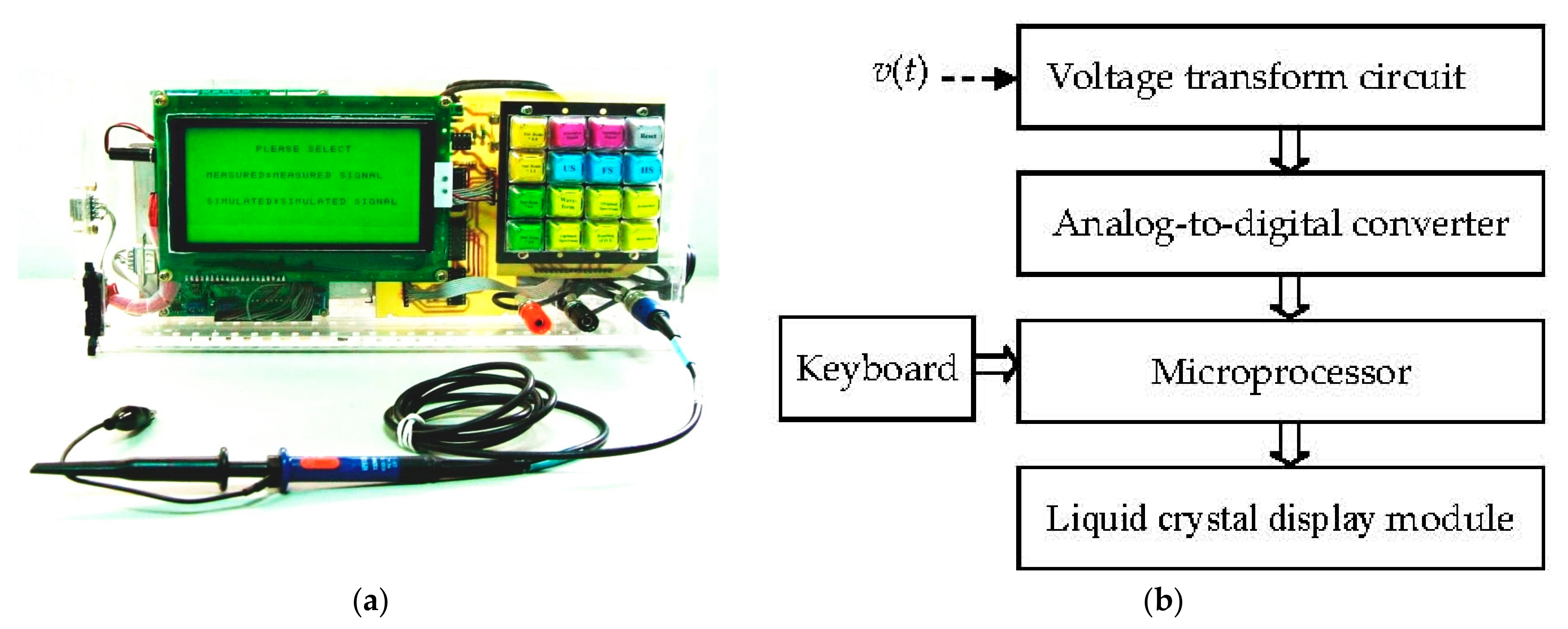
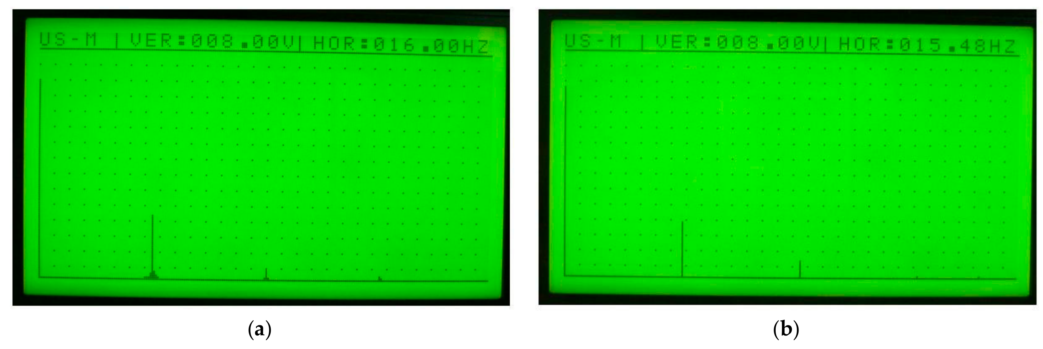
3.6. Implementation in Instrument
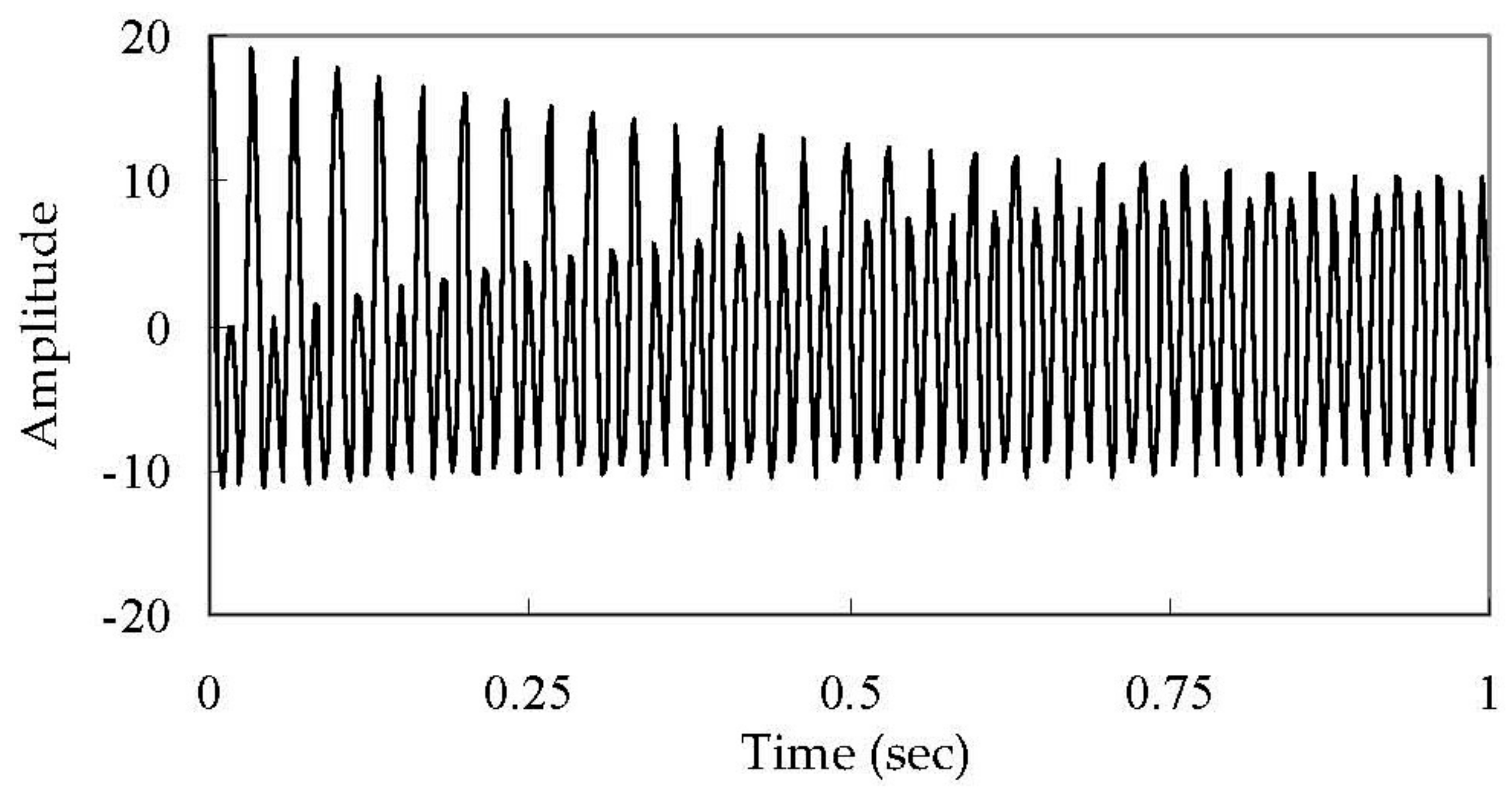
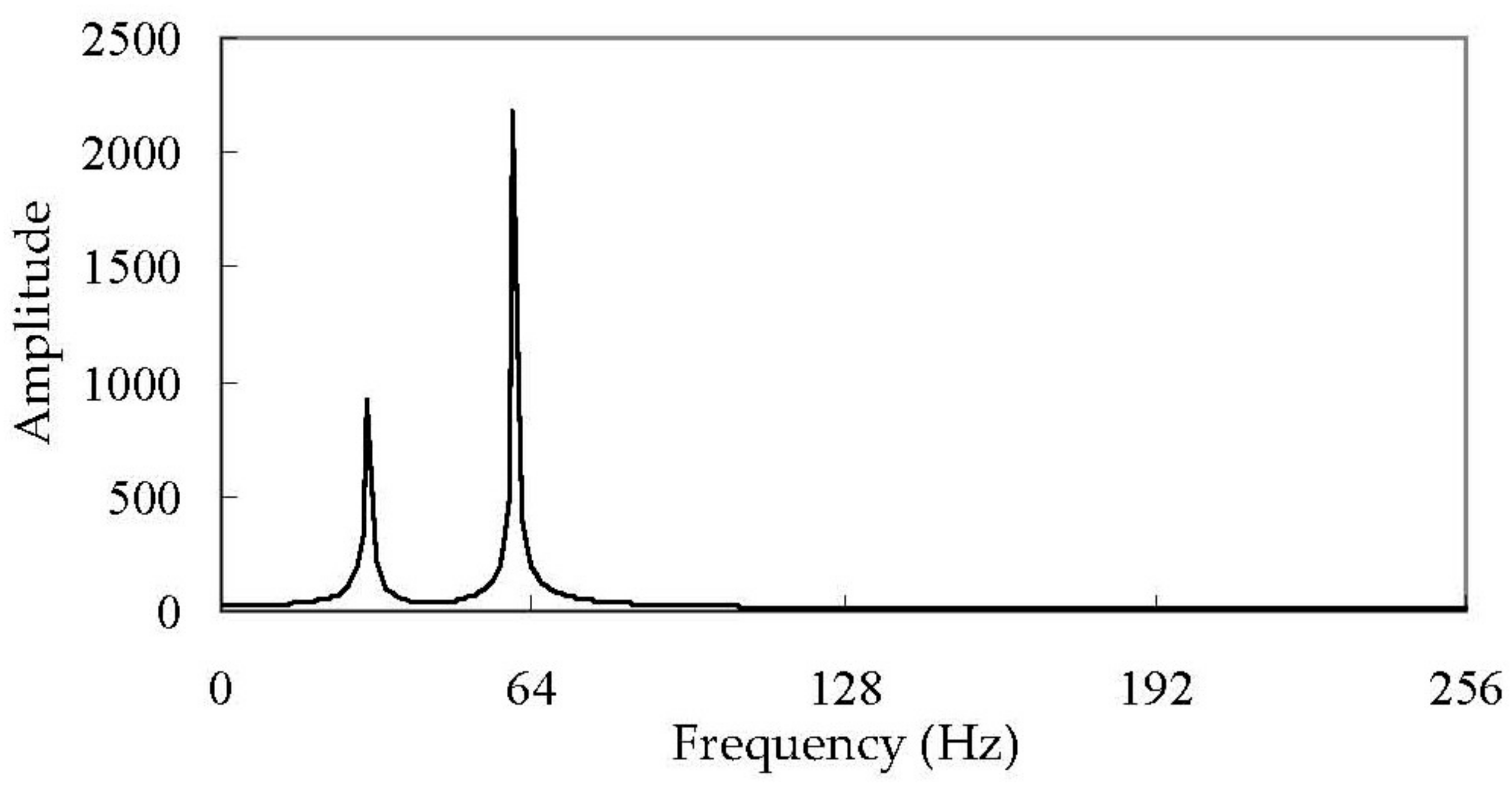
A practical instrument implementing this method is also demonstrated in this paper, shown in Figure 12a. This instrument is based on the TI TMS320LF2407 DSP microprocessor, and consists of five modules [29]: The voltage-transform circuit, analog-to-digital converter, microprocessor, keyboard module, and liquid-crystal-display module, as shown in Figure 12b. The function of the voltage-transform circuit is to transform the utility nominal voltage of alternate current (AC 110 V) into an input voltage that meets the specifications of the analog-to-digital converter (0–5 V). In this converter, the sample rate is set at 1024 samples/s, with the number of samples set at 1024 and a sample period of 1.0 s. The 8-bit analog-to-digital converter has a resolution of 19.6 mV for a 5 V signal voltage. In this instrument, the functions of measurement, calculation, storage, and display are also included.
The analysis of a full-wave-rectified voltage is used as the example. Figure 13a shows the spectrum from FFT. The signal causes obvious leakage effects on the spectrum. Figure 13b is the results of the optimal spectrum, whose scale is close to that in Figure 13a. However, after scale adjustment, the energy of each harmonic has been located at the identical bin, and the leakage effect has been decreased to a minimum.

3.7. Application

Due to the diversity of signals, different analysis methods are available for different signal structures.
In the engineering field, the responses of analyzed systems often contain a few important frequency components, and the signal structure is relatively simple [30,31,32,33]. An exact result is therefore the requirement when analyzing this type of signal, and the optimized effect will aid in the analysis of these signals. The proposed method uses two parameters to optimize the spectrum. When the signal structure is more complex, the optimization result is less obvious. At this point, a small number of specific components can be analyzed, and local optimization results can still be obtained.
Biological signals from equipment such as the electrocardiogram (EKG) [34], electroencephalogram (EEG) [35], electromyography (EMG) [36], pulse pressure [37], phonocardiogram [38] and others, possess characteristics of large variation range, are non-stationary, have high time-variance rates, many interference factors, and are relatively complex structures. Because of the large range of variation in these signals, statistical analysis is often used to verify their significance.
In biological signals, EKG, pulse pressure, and phonocardiogram [39] can easily derive a period in the time domain, so these signals are often explained in the time domain.
In biological signals, EEG [40] and EMG have no obvious features in the time domain. Such signals are often represented as a spectrum, as the significant features can be observed in the frequency domain; however, the frequency components of such signals are also quite complex. In such signals, the instability of the signal far exceeds the leakage effect, and the optimization method will not assist in the analysis of these signals.

4. Conclusions

This paper proposes an optimization-based method for spectrum analysis, which adjusts the frequency scale to match the signal characteristics. When the frequency scale matches the signal characteristics, the leakage effect will be decreased to a minimum, and the spectrum analysis will reach an optimum. The capabilities of this method have been evaluated, and it has the following features:
(1)
Extensive suitability: This method can be used for signals with complex exponential components, but is not limited to periodic signals.
(2)
Preserving original characteristics: The optimization process involves changing the frequency scale, after which the original characteristics will be completely preserved.
(3)
Close scale: The scale parameters of the optimal spectrum are near to the original ones, which makes the optimization results obtainable through a fine-tuning modality.
(4)
Directly obtaining parameters for periodic components: In the optimal spectrum, the amplitude of a periodic component concentrates at an identical bin whose parameters can be read directly.
(5)
Component property re-organization: In the optimal spectrum, the non-periodic component will cause non-zero bandwidth from its damping. Therefore, the periodicity or non-periodicity of a component can be recognized by observing whether non-zero bandwidth exists or not.
A real instrument is also demonstrated in this paper, so that the practical application of the method presented can be verified.

Author Contributions

R.-C.W. conceived of the feature extraction method, wrote programs, and analyzed the results; L.-J.H. acquired the funding, realized the instrument, performed the experiments, and drafted the manuscript; all authorship read and approved the final manuscript.

Funding

This research was funded by Kaohsiung Municipal Ta-Tung Hospital Grant Number KMTTH-106-038.

Conflicts of Interest

The authors declare no conflict of interest.

References

  1. Abbasi, A.; Seifi, A. Fast and perfect damping circuit for ferroresonance phenomena in coupling capacitor voltage transformers. Electr. Power Compon. Syst. 2009, 37, 393–402. [Google Scholar] [CrossRef]
  2. Tsai, J.-I.; Chen, C.-C.; Zhan, T.-S.; Wu, R.-C. Depressing turbine-generator supersynchronous torsional torques by using virtual inertia. In Proceedings of the ICCESSE 2010, Tokyo, Japan, 26–28 May 2010. [Google Scholar]
  3. Viana, F.A.C.; Steffen, V.J. Multimodal vibration damping through piezoelectric patches and optimal resonant shunt circuits. J. Braz. Soc. Mech. Sci. Eng. 2006, 28, 293–310. [Google Scholar] [CrossRef]
  4. Tkáča, L.; Schauer, F. Energy balance in real electronic RLC circuits by remote experimentation. Procedia Soc. Behav. Sci. 2013, 89, 158–162. [Google Scholar] [CrossRef]
  5. Yan, B.; Wang, K.; Hu, Z.; Wu, C.; Zhang, X. Shunt damping vibration control technology: A review. Appl. Sci. 2017, 7, 494. [Google Scholar] [CrossRef]
  6. Iglesias, A.; Munoa, J.; Ciurana, J.; Dombovari, Z.; Stepan, G. Analytical expressions for chatter analysis in milling operations with one dominant mode. J. Sound Vib. 2016, 375, 403–421. [Google Scholar] [CrossRef]
  7. Otto, A.; Rauh, S.; Kolouch, M.; Radons, G. Extension of Tlusty’s law for the identification of chatter stability lobes in multi-dimensional cutting processes. Int. J. Mach. Tool Manuf. 2014, 82–83, 50–58. [Google Scholar] [CrossRef]
  8. Sanaati, B.; Kato, N. A study on the effects of axial stiffness and pre-tension on VIV dynamics of a flexible cylinder in uniform cross-flow. Appl. Ocean Res. 2012, 37, 198–210. [Google Scholar] [CrossRef]
  9. Gu, J.; Wang, Y.; Zhang, Y.; Duan, M.; Levi, C. Analytical solution of mean top tension of long flexible riser in modeling vortex-induced vibrations. Appl. Ocean Res. 2013, 41, 1–8. [Google Scholar] [CrossRef]
  10. Lee, J.; Allen, D. Vibration frequency and lock-in bandwidth of tensioned, flexible cylinders experiencing vortex shedding. J. Fluid Struct. 2010, 26, 602–610. [Google Scholar] [CrossRef]
  11. Girgis, A.A.; Ham, F.M. A quantitative study of pitfalls in the FFT. IEEE Trans. Aerosp. Electron. Syst. 1980, 16, 434–439. [Google Scholar] [CrossRef]
  12. Moo, C.-S.; Chang, Y.-N.; Mok, P.P. A digital measurement scheme for time-vary transient harmonics. IEEE Trans. Power Deliv. 1995, 10, 588–594. [Google Scholar] [CrossRef]
  13. Lin, H.C. Inter-harmonic identification using group-harmonic. IEEE Trans. Power Electron. 2008, 23, 1309–1319. [Google Scholar]
  14. Agrež, D. Weighted multi-point interpolated DFT to improve amplitude estimation of multi-frequency signal. IEEE Trans. Instrum. Meas. 2002, 51, 287–292. [Google Scholar] [CrossRef]
  15. Qian, H.; Zhao, R.; Chen, T. Interharmonics Analysis based on interpolating windowed FFT algorithm. IEEE Trans. Power Deliv. 2007, 22, 1064–1069. [Google Scholar] [CrossRef]
  16. Wen, H.; Teng, Z.; Wang, Y.; Zeng, B.; Hu, X. Simple interpolated FFT algorithm based on minimize sidelobe windows for power-harmonic analysis. IEEE Trans. Power Electron. 2011, 26, 2570–2579. [Google Scholar] [CrossRef]
  17. Wen, H.; Zhang, J.; Meng, Z.; Guo, S.; Li, F.; Yang, Y. Harmonic estimation using symmetrical interpolation FFT based on triangular self-convolution window. IEEE Trans. Ind. Inform. 2015, 11, 16–26. [Google Scholar] [CrossRef]
  18. Nuttall, A.H. Some windows with very good sidelobe behavior. IEEE Trans. Acoust. Speech Signal Process. 1981, 29, 84–91. [Google Scholar] [CrossRef] [Green Version]
  19. Mottaghi-Kashtiban, M.; Shayesteh, M.G. New efficient window function, replacement for the hamming window. IET Signal Process. 2011, 5, 499–505. [Google Scholar] [CrossRef]
  20. Yang, J.-Z.; Yu, C.-S.; Liu, C.-W. A new method for power signal harmonic analysis. IEEE Trans. Power Deliv. 2005, 20, 1235–1239. [Google Scholar] [CrossRef]
  21. Lu, S.-L. Application of DFT filter bank to power frequency harmonic measurement. IEE Proc. Gener. Transm. Distrib. 2005, 152, 132–136. [Google Scholar] [CrossRef]
  22. Wu, R.-C.; Tsao, T.-P. The optimization of spectrum analysis for digital signal. IEEE Trans. Power Deliv. 2003, 18, 398–405. [Google Scholar] [CrossRef]
  23. Bertocco, M.; Offelli, C.; Petri, D. Analysis of damped sinusoidal signals via a frequency-domain interpolation algorithm. IEEE Trans. Instrum. Meas. 1994, 43, 245–250. [Google Scholar] [CrossRef]
  24. Chang, G.W.; Chen, C.-I. An accurate time-domain procedure for harmonics and interharmonics detection. IEEE Trans. Power Deliv. 2010, 25, 1787–1797. [Google Scholar] [CrossRef]
  25. Claeys, T.; Vanoost, D.; Peuteman, J.; Vandenbosch, G.A.E.; Pissoort, D. Removing the spectral leakage in time-domain based near-field scanning measurements. IEEE Trans. Electromagn. Compat. 2015, 57, 1329–1337. [Google Scholar] [CrossRef]
  26. Wu, R.-C.; Tsao, T.-P. Theorem and application of adjustable spectrum. IEEE Trans. Power Deliv. 2003, 18, 372–376. [Google Scholar] [CrossRef]
  27. Girgis, A.A.; Clapp, M.C.; Makram, E.B.; Qiu, J.; Dalton, J.; Catore, R. Measurement and characterization of harmonics and high frequency distortion for a large industrial load. IEEE Trans. Power Deliv. 1990, 5, 427–434. [Google Scholar] [CrossRef]
  28. Oppenheim, A.V.; Schafer, R.W. Discrete-Time Signal Processing, 2nd ed.; Prentice-Hall: Upper Saddle River, NJ, USA, 1999; pp. 40–47. ISBN 0137549202. [Google Scholar]
  29. Mortensen, A.N.; Johnson, G.L. A power system digital harmonic analyzer. IEEE Trans. Instrum. Meas. 1988, 37, 37–540. [Google Scholar] [CrossRef]
  30. Tsai, J.-I.; Lu, G.-C.; Wu, W.-C.; Hsueh, C.-Y.; Wu, R.-C. Torque vibrations on the mechanism of wind turbine generators excited by balanced network faults. In Proceedings of the APPEEC 2012, Shanghai, China, 27–29 March 2012. [Google Scholar]
  31. Ji, H.; Qiu, J.; Zhang, J.; Nie, H.; Cheng, L. Semi-active vibration control based on unsymmetrical synchronized switching damping: Circuit design. J. Intell. Mater. Syst. Struct. 2015, 27, 1106–1120. [Google Scholar] [CrossRef]
  32. Totisa, G.; Albertellib, P.; Tortac, M.; Sortinoa, M.; Monnob, M. Upgraded stability analysis of milling operations by means of advanced modeling of tooling system bending. Int. J. Mach. Tool Manuf. 2017, 113, 19–34. [Google Scholar] [CrossRef] [Green Version]
  33. Chen, W.; Li, Y.; Fu, Y.; Guo, S. On mode competition during VIVs of flexible SFT’s flexible cylindrical body experiencing lineally sheared current. Procedia Eng. 2016, 166, 190–201. [Google Scholar] [CrossRef]
  34. Reed, M.J.; Robertson, C.E.; Addison, P.S. Heart rate variability measurements and the prediction of ventricular arrhythmias. QJM-Int. J. Med. 2005, 98, 87–95. [Google Scholar] [CrossRef] [PubMed] [Green Version]
  35. Lin, L.-C.; Ouyang, C.-S.; Chiang, C.-T.; Wu, R.-C.; Wu, H.-C. Cumulative effect of transcranial direct current stimulation in patients with partial refractory epilepsy and its association with phase lag index-A preliminary study. Epilepsy Bevav. 2018, 84, 142–147. [Google Scholar] [CrossRef] [PubMed]
  36. Sadikoglua, F.; Kavalcioglub, C.; Dagmanc, B. Electromyogram (EMG) signal detection, classification of EMG signals and diagnosis of neuropathy muscle disease. Procedia Comput. Sci. 2017, 120, 422–429. [Google Scholar] [CrossRef]
  37. Franklin, S.S.; Wong, N.D. Pulse pressure: How valuable as a diagnostic and therapeutic tool? J. Am. Coll. Cardiol. 2016, 67, 404–406. [Google Scholar] [CrossRef] [PubMed]
  38. Obaidat, M.S. Phonocardiogram signal analysis: Techniques and performance comparison. J. Med. Eng. Technol. 1993, 17, 221–227. [Google Scholar] [CrossRef] [PubMed]
  39. Taebi, A.; Hansen, A.M. Time-frequency distribution of seismocardiographic signals: A comparative study. Bioengineering 2017, 4, 32. [Google Scholar] [CrossRef] [PubMed]
  40. Lin, L.-C.; Ouyang, C.-S.; Chiang, C.-T.; Yang, R.-C.; Wu, R.-C.; Wu, H.-C. Early prediction of medication refractoriness in children with idiopathic epilepsy based on scalp EEG analysis. Int. J. Neural Syst. 2014, 24, 1450023. [Google Scholar] [CrossRef] [PubMed]
Figure 1. Reference data for parameter estimation.
Energies 11 01841 g001
Figure 2. Leakage effects from different frequency biases.
Energies 11 01841 g002
Figure 3. Frequency scale adjustment.
Energies 11 01841 g003
Figure 4. Waveform of Equation (24).
Energies 11 01841 g004
Figure 5. Analysis result of fast Fourier transform (FFT) for Equation (24).
Energies 11 01841 g005
Figure 6. Relation between sampling number and frequency biases.
Energies 11 01841 g006
Figure 7. Optimal scale parameter searching.
Energies 11 01841 g007
Figure 8. New signal.
Energies 11 01841 g008
Figure 9. Optimization result (N’ = 510, Ss = 0.0663).
Energies 11 01841 g009
Figure 10. Complete optimized spectrum of Equation (24).
Energies 11 01841 g010
Figure 11. Analyzed results from different methods.
Energies 11 01841 g011
Figure 12. Instrument for optimized analysis of spectrum. (a) Practical work; and (b) schematic block diagram.
Energies 11 01841 g012
Figure 13. Comparison of analysis results. (a) Result from FFT; (b) result from the optimal spectrum.
Energies 11 01841 g013
Table 1. Results of parameter estimation.
ComponentParameterReal ValueAnalysis Result
Component 1Frequency30.230.177
Damping−2.5−2.59
Amplitude1010.49
Phase00.044
|X’(p)|939.95956.66
Component 2Frequency60.360.303
Damping0−0.04
Amplitude1010.062
Phase0−0.011
|X’(p)|25602557.09
Table 2. Presentations from different scale parameters.
ComponentReal FrequencyResult of FFTResult of Optimal Scale Parameters (N’, Ss)
(510, 0.066)(527, 0.073)
Component 130.23030.18130.188
Component 260.36060.29960.306
Table 3. Analysis result for Equation (24) in different frequency domains.
ComponentParameterReal ValueResult in Positive Frequency DomainResult in Negative Frequency Domain
Component 1Frequency30.230.191−30.207
Damping2.52.5542.46
Amplitude1010.29110.088
Phase00.010.024
Component 2Frequency60.360.308−60.301
Damping00.0360.036
Amplitude1010.0329.994
Phase0−0.030.013

