An Iterative Reduced KPCA Hidden Markov Model for Gas Turbine Performance Fault Diagnosis


1
Jiangsu Province Key Laboratory of Aerospace Power Systems, College of Energy & Power Engineering, Nanjing University of Aeronautics and Astronautics, Nanjing 210016, China
2
Aviation Motor Control System Institute, Aviation Industry Corporation of China, Wuxi 214063, China
*
Author to whom correspondence should be addressed.
Energies 2018, 11(7), 1807; https://doi.org/10.3390/en11071807
Submission received: 5 June 2018
/
Revised: 3 July 2018
/
Accepted: 5 July 2018
/
Published: 10 July 2018
Abstract
:To improve gas-path performance fault pattern recognition for aircraft engines, a new data-driven diagnostic method based on hidden Markov model (HMM) is proposed. A redundant sensor somewhat interferes with fault diagnostic results of the HMM, and it also increases the computational burden. The contribution of this paper is to develop an iterative reduced kernel principal component analysis (IRKPCA) algorithm to extract fault features from original high-dimension observation without large additional calculation load and combine it with the HMM for engine gas-path fault diagnosis. The optimal kernel features are obtained by iterative sequential forward selection of the IRKPCA, and the features with lower dimensions are contracted through a trade-off between the fault information and modeling data scale in reduced kernel space. The similarity degree is designed to simplify the HMM modeling data using fault kernel features. Test results show that the proposed methodology brings a significant improvement in diagnostic confidence and computational efforts in the applications of a turbofan engine fault diagnosis during its steady and dynamic process.
1. Introduction
The gas turbine engine is the power source of aircraft, and its reliability directly affects aircraft safety and performance [1]. The engine is an easy-fault piece of machinery since it has complex structure and runs in harsh operating conditions. During the course of an engine’s life, various physical failures might happen, such as corrosion, erosion, fouling, and foreign object damage [2,3]. These failures lead to gas-path performance degradation, either gradually or abruptly, which is recognized as engine gas-path fault and is greatly harmful to flight safety [4,5]. For the purpose of enhancing operating reliability and reducing maintenance costs of aircraft propulsion systems, engine gas-path fault diagnosis technology has attracted interest.
Generally speaking, gas turbine fault diagnosis approaches are divided into model-based and data-driven ones [6,7]. Variants of Kalman filters are the typical model-based diagnostic methods for gas turbine engines [8,9]. It requires a reliable engine model, which relies on physical characteristics and aero-thermodynamic theory. The engine modeling uncertainties and operation non-linearity during the transient process negatively affects the performance of model-based technologies [10]. Engine-to-engine variation makes it difficult for the general engine model to represent every individual engine. In addition, the observability of general Kalman filters relates to the number of sensor measurements and their types, and it cannot recognize fault patterns as available sensors less than health parameters.
The data-driven approach is another important method of fault diagnosis for complex non-linear systems, especially in the rich data circumstance [11,12,13]. It depends on the collected data of fault modes but not an accurate mathematical model of a gas turbine engine. It is particularly suitable to a complex strong non-linear system, and it is not limited to the sensor measurement number. In the data-driven field, much attention has been paid to neural network approaches, which are theoretically developed from empirical risk minimization with simple mathematical expressions [8]. Bartolini applied neural networks to micro gas turbines, and then Amozegar developed an ensemble of dynamic neural network identifiers for engine fault detection and isolation [14,15]. The desirable topological structure of a neural network is usually selected by experience, and the diagnostic performance by a neural network easily fluctuates with stochastic measurement noise.
Different from the neural network approaches, the hidden Markov model (HMM) is a classic data-driven fault diagnosis for non-linear stochastic systems [16]. The HMM has rigorous theoretical deduction and definite model structure [17]. HMM statistical characteristics in modeling and classification makes it outperform fault pattern recognition for a mechanical system with clear randomness and uncertainties [18]. However, it is noted that the HMM’s computational cost increases dramatically when the measurement dimension increases. The sensor data from various operating cross-sections for engine gas-path fault diagnosis is usually complex and physically correlative in transient process in the flight envelope. Consequently, it is necessary to extract fault features from raw measurement sequences to decrease test data dimensions and simplify the HMM structure.
Principal component analysis (PCA) is introduced into the HMM to extract fault features to reduce computational effort. PCA is achieved by projecting the linear data matrix onto an uncorrelated subspace with less information loss, but its performance is reduced in the plant with strong non-linearity. Kernel-PCA (KPCA) is developed to overcome shortcomings of conventional PCA-to-linear issues [19,20]. Provided a kernel matrix (an n × n matrix where n is the number of the dataset) to map an original dataset into the feature space, the KPCA computational complexity is O(n3) in the principal component feature extraction. Taouali proposed a novel RKPCA to improve the sparsity capability [21], but it is difficult to balance the useful information capacity and data scale to reach the appropriate sample number.
To improve fault diagnostic confidence and computational efforts, a novel fault diagnostic approach is proposed using the combination of iterative reduced KPCA and HMM for engine gas-path fault diagnosis. In this paper, the IRKPCA is developed with a sample-reduction mechanism, which is designed to decline the redundant information in the initial observation sequences for gas-path fault feature extraction. The similarity degree and forward kernel inverse are employed to simplify the sample data, and then the kernel fault feature by the IRKPCA is used by the HMM to perform gas-path fault pattern recognition. The systematical tests are carried out to evaluate fault diagnosis performance of the proposed methodology, and it runs on a two-spool turbofan engine simulation in the steady and transient process at various cycle numbers during its life. The results indicate the superiority of the IRKPCA-HMM, and it supports our viewpoints.
The remainder of paper is organized as follows. The IRKPCA is developed from the basic KPCA, and the comparisons of the involved KPCAs are followed by feature extraction performance using benchmark datasets in Section 2. In Section 3, the IRKPCA-HMM is presented by the combination of IRKPCA and HMM to simplify the fault diagnostic model using reduced-kernel fault features. Simulation and analysis are given on a turbofan engine in dynamics for gas-path fault diagnosis in Section 4. Section 5 draws a conclusion and discusses future research directions.
2. IRKPCA-Based Feature Extraction Algorithm
2.1. KPCA
As the non-linear extension of PCA, KPCA has been applied to various engineering fields and exhibited satisfactory performance in complicated non-linear systems [19,22]. The kernel transformation of the KPCA maps the measured data space to higher-dimension feature space. Given a set of N mean-variance scaled training data, , ∈, , and L is the original dimension of training measurement. The covariance matrix in the feature space F is
where transformation matrix is a non-linear map from input vector into H-dimensional feature space F. Non-zero eigenvectors γ of the covariance matrix C is calculated by eigenvalue decomposition
where λ is the eigenvalues of C in feature space. Combine two expressions in Equation (2) and multiply the kernel matrix in both sides, and we can obtain
Then, a kernel matrix K = {kij} with the dimension of N × N is introduced to achieve the inner product in non-linear feature space
A radial basis kernel is used for Kernel transformation, and σ is a dispersion factor. The kernel matrix K is centralized before kernel transformation
where I is an identity matrix with the size of N × N. Then, Equation (3) is specified as
The kernel principal components are selected as the p largest positive eigenvalues , and their eigenvectors ɛ1, …, ɛp form the kernel principal component set. The projection parameter of a new data onto the eigenvectors in the principal component set is called the KPCA-transformed feature variable. The i-th feature zi for is expressed
From Equation (7), the kernel matrix is computed to obtain the feature vector for each sample in training dataset. The burden of computation and storage would be dramatically serious for drawing fault features as the increase of kernel matrix calculation number and the sample data accumulation. For these purposes, an iterative reduced KPCA (IRKPCA) is developed from the KPCA algorithm.
2.2. IRKPCA
Given the selected samples set from the training dataset , Ns means the selected sample number. The base vectors in feature subspace related to the selected samples are sufficient to express the whole transformed data in feature space. Thus, the mapping estimate of any sample vector can be represented by a linear combination of these base vectors
where ai is the coefficient vector on the feature subspace basis denoted as . A new objective function to find these coefficients is designed, and it includes two minimization elements: the estimated mapping errors and coefficient vector norm. The objective function is expressed as
where 𝜌 is the regularization parameter to weight off the estimation error and coefficient scales. The former part indicates that the modeling-variable mapping is as close as possible to the real mapping, and the latter one compacts the scales. Let , we have
where Is is an identity matrix of the size of s × s. Combining Equations (9) and (10), the solution of minimization Ji can be rewritten
where Kss represents the kernel matrix of the selected vectors, and Ksi is the dot product between and the selected base vectors, Ksi = [k(x1,xi), …, k(xs,xi)]T. Since the calculation procedure of objective function is treated to each sample in the training dataset, the overall objective function is defined by
Equation (12) can be rewritten as
The sample reduction procedure is an iterative sequential forward process. The sample chooses preforms from the training dataset at each step of the procedure, which are combined with the prior selected ones to generate the optimal objective function of Equation (13). The procedure stops as the mean of overall objective is no longer increasing clearly when the sample is added. The mean residual is given by
To reduce the number of training sample, the similarity degree is used. The similarity degree between a new sample and the selected samples is
Kernel matrix inverse is calculated when a new training sample is selected during the iteration. It is very time-consuming to repeatedly calculate the Kss inverse. The forward kernel inverse strategy is used to compute the (s + 1)-th sample given base vectors and Rs = (Kss+ ρIs)−1
Provided an invertible matrix A, and matrices D, V, U, we have
Since the matrix Rs has been obtained at the s-th iteration, Rs can be directly acquired by applying Equation (17) to Equation (16) for the matrix inversion
where , , and the kernel inverse number becomes 1 as a new training sample is considered. The reduction scheme of IRKPCA training sample is developed by simplifying training data number for fault feature extraction. In the IRKPCA, the sample similarity degree is checked in advance, and the sample is such that the similarity index larger than its threshold is deleted. The forward kernel inverse strategy is employed to produce the matrix Rs+1 with respect to new training data.
2.3. Feature Extraction Performance Test
The benchmark datasets from UCI Machine Learning [23] are used to validate feature extraction performance of the basic KPCA and proposed IRKPCA. The six datasets include Iris, Wine, Glass, E.coli, Balance and Vehicle. The feature number (#Feature), the number of classes (#Class) and sample number (#SN) of each dataset are listed in Table 1.
The comparisons of basic KPCA and IRKPCA are investigated from reduced features, discriminative power, sparsity, and reduced time in Table 2. The reduced feature number depicts the principal component size after feature extraction by the KPCA. Discriminative power contains the mean correct classification ratio and standard errors using the reduced features in the transformed space. Sparsity is expressed by 2-norm/1-norm (L2/L1), and the larger L2/L1 value is more in favor of classification [24,25]. The reduced-dimension time gives the computational efforts of dataset transformation from the original measurement space to feature space. The regularization parameter ρ and kernel parameter σ are yielded separately from the bound of [2–3, 23] and [20, 210] by the interval 2 times.
From Table 2, we can see that both KPCA algorithms reduce the feature number, and the number by IRKPCA is less than that by KPCA in the most examined datasets. In terms of the discriminate power index, the IRKPCA produces more than 2.70% and 2.89% of mean correct ratio compared to KPCA in the E.coli and Balance datasets, respectively. The differences of mean correct ratios by the two KPCAs in the rest of the datasets are no more than 1%. The indices L2/L1 by IRKPCA is slightly larger than those by KPCA except in the Glass dataset, so the former produces less information loss than the learning feature. The KPCA generates one magnitude larger reduced time than IRKPCA. The reduced time of KPCA increases faster with the sample size, and the indices are 1.2387 s by KPCA and 0.0645 s by IRKPCA in the Vehicle dataset. The IRKPCA consumes less computational time and owns a lower feature number without discriminative power reduce compared to KPCA. Hence, it implies that the IRKPCA might be a better candidate for gas-path fault feature extraction. Figure 1 shows the extraction effect on benchmark datasets of Iris and Wine by the proposed IRKPCA method. The first three dimensions of benchmark datasets are presented in the form of scatter plots in Figure 1, and the points with the same color belongs to the same cluster. From Figure 1 we can see that the distance of different color points increases after the dimension transformation by the IRKPCA. The processed datasets are more easily distinguished than the original dataset in scatter plots, and it supports further classification.
3. IRKPCA-HMM Based Structure
3.1. Hidden Markov Model
Hidden Markov model is extended from Markov chains to yield inferential statistical information on a state sequence [26,27]. It comprises a finite hidden state number, and each state relates to an observation at a time point. There are two kinds of probabilities of every hidden state: transition probability and observation probability. HMM have double stochastic processes: the stochastic transition from one hidden state to another one with transition probability and the stochastic output observation generated from every hidden state with observation probability.
The state sequence of HMM is unobservable, but it can be estimated from the observation sequence. Let hidden state sets and observation vector with , where M is the number of hidden states, N is the number of observation per state and T is the length of observation sequence. The variable () indicates the hidden state, and () the observation at time t. In general, the compact definition λ = (π, A, B) is used to specify an HMM model, and it includes three components: state transition probability matrix A, observation probability matrix B, and initial state distribution π.
An initial state distribution π illustrates the probability of the starting hidden state si (t = 0)
where πi = Pr(q0 = si), 1 ≤ i ≤ M.
A transition probability A contains the element aij
where aij is the probability of transition from one hidden state si at time t to another hidden state sj at time t + 1, and it follows aij = Pr(qt+1 = sj|qt = si), 1 ≤ i, j ≤ M. The observations are emitted from each state according to the conditional probability, bi(vj) = Pr(ot = vj|qt = si), which is represented as a matrix B{bi(oj)} as well. The elements of B evidently satisfy the constraints:
The Baum-Welch algorithm is used to obtain the topological parameters of HMM, where an iterative calculation is implemented to maximize the observed sequence probability Pr(X|λ) from an initial λ. The observed sequence XT×H = [x1, x2, …, xT]T is divided into two sections: Xt×H = [x1, x2, …, xt]T with t measurement data number, and X(T−t)×H = [xt+1, xt+2, …, xT]T with T − t. H is the dimension of measurement vector. Two probabilities corresponding to the forward variable and backward variable are computed. The former is denoted by the probability of observing the partial measurement data Xt×H ending in the state sj, and the latter by the probability of observing the remaining data X(T−t)×H as the state si. The forward variable αt(j) is
where α1(i) = πi. bi(x1), 1 ≤ i ≤ M. The backward variable βt(i) is
where βT(i) = 1, 1 ≤ i ≤ M. The detailed Baum-Welch algorithm to obtain the probability of sequence O can be referred to in paper [28]. The scalar quantization is to generate the partition vector and the codebook vector according to the quantization distortion of the input before training HMM [29].
The observation sequence of HMM is formed by measurement data from various sensors, which are equipped along a gas path to depict engine operation. As mentioned earlier, redundant information of various operating data will increase fault diagnosis difficulty. The larger dimension of measurement vector xi leads to more complex HMM topology [5,19]. It would not only increase the computational time of forward-backward procedure in Baum-Welch algorithm but also negatively impact on classification accuracy.
3.2. IRKPCA-HMM Algorithm
Gas-path fault feature extraction based on the IRKPCA is combined with HMM for fault diagnosis in this section. The reduced observation sequence X*T×R = [x*1, x*2, …, x*T]T with R feature dimensions (R < H) is generated from the original sequence XT×H. Thus, the re-estimation process of HMM with the new sequence X*T×R is as follows
where is k-th forward variable, and is k-th backward variable. In IRKPCA-HMM test phase, Equation (26) is specified as
The log-likelihood probability (LL) is a fault index defined by the logarithm calculation to in Equation (27). The larger LL indicates the greater consistency of observation sequence to the HMM.
The IRKPCA-HMM achieves gas-path fault diagnosis in the lower dimension feature space from the original measurement space, and it decreases the calculation effort not only in the training process but also in testing process. The IRKPCA-HMM algorithm schematic is presented for fault diagnosis of aero engines in Figure 2.
The proposed IRKPCA-HMM procedure is as follows:
- (1)
- Initialization.Set initial kernel parameters, regulation parameter and information loss threshold. Select the number of hidden states and observation states, and topological structure of HMM.
- (2)
- Search optimal samples by iterations.
- (2.1.)
- The original training sample set X0, and let the dataset .
- (2.2.)
- Select the first optimal sample. Calculate the objective function Equation (13) for each sample, and the sample x1 with the maximum objective value is added into the sample dataset Xs, .
- (2.3.)
- Compute the sample similarity degree. The similarity degree is computed between the selected sample in Xs and rest samples xi in . If sample similarity degree is larger than similarity threshold, then , i = I + 1, and continue until the rest samples are all checked.
- (2.4.)
- Calculate the objective Equation (18) for each sample and select the sample of maximum objective value xi. Compute the mean objective residual as Equation (14) for the selected optimal sample xi. If the sample mean objective residual is larger than the difference threshold, go to 1.3, else continue.
- (3)
- Principal component computation in kernel space.
- (3.1.)
- Calculate the centralized kernel matrix K with selected samples.
- (3.2.)
- Compute eigenvectors with corresponding eigenvalues .
- (3.3.)
- Choose the p largest eigenvalues until //information loss threshold.
- (4)
- Online fault feature extraction for testing data {}.
- (4.1.)
- Calculate Ksi(xnew) = [k(x1, xnew), …, k(xs, xnew)]T.
- (4.2.)
- Calculate the features according to Equation (7).
- (5)
- HMM modeling with reduced observation.
- (5.1.)
- Set initial number of hidden states, observation states and choose topology structure of HMM.
- (5.2.)
- Re-estimate parameter using Equations (24) and (25).
- (5.3.)
- Form the HMM libraries for gas-path fault modes.
4. IRKPCA-HMM Based Engine Gas-Path Fault Diagnosis
The proposed IRKPCA-HMM approach to gas-path fault diagnosis is tested on a virtual two-spool turbofan engine developed by the component-level engine model [30,31]. The examined turbofan engine is mainly composed of inlet, fan, compressor, bypass, combustor, high-pressure turbine (HPT) and low-pressure turbine (LPT), mixer and nozzle, and it is illustrated in Figure 3. The inlet supplies airflow into the fan, and then the air is divided to two streams: one flowing into the compressor and the other passing through the bypass. Air leaving the compressor moves to the combustor, where fuel is injected and burns to produce hot gas to drive the turbines. The fan and compressor are driven by the LPT and HPT, respectively. Gas from LPT and air from bypass mix in the mixer, and then leaves the engine through the nozzle. Closed-loop control strategy of spool speed is applied to aero engine with safety protection [32]. The engine station numbers in Figure 3 are as follows: inlet exit marked by 2, compressor inlet by 22, compressor exit by 3, HPT entrance by 43, LPT entrance by 5, and LPT exit by 6.
The data are generated from the numerical engine model [33,34] to evaluate the involved methods in the steady behavior of the maximum power operation and transient behavior including acceleration and deceleration. The involved engine parameters are reported in Table 3. The control variables include fuel flow Wf and Nozzle area A8, which define the operating point of the engine. The health parameters are unmeasurable and represent engine gas-path health, containing indicators of fan efficiency SE1, fan flow SW1, compressor efficiency SE2, compressor flow SW2, HPT efficiency SE3, HPT flow SW3, LPT efficiency SE4, and LPT flow SW4. The available measurements are used to calculate health parameters, and they are low-pressure spool speed NL, high-pressure spool speed NH, compressor inlet temperature T22, compressor inlet pressure P22, compressor outlet pressure P3, compressor outlet temperature T3, LPT inlet temperature T43, LPT inlet pressure P43, LPT outlet pressure P5 and mixing chamber inlet temperature T6 [35]. The maximum power point on the ground is defined as corrected percentage of high-pressure spool speed NHcor = 100%, and corresponds to the corrected normalized values of engine control variables: fuel flow Wf = 100%, nozzle area A8 = 47%. The measurement noise follows time-uncorrelated zero-mean Gaussian noise, and the magnitude of these noises can be referred to in paper [36].
Both gradual and abrupt performance deterioration causes health parameter variations. The health parameters resulting from performance gradual degradation is long term, and all health parameters synchronously diverge from their nominal quantities with the cycle number increase. It starts from a healthy engine (all health parameters at their nominal values) at initial cycle number CN = 0, and with the linearly deviation at the end of cycle number CN = 6000. The first factory overhaul occurs at one quarter of the engine’s whole lifetime, and three cycle number points before this overhaul, including CN = 0, CN = 807 and CN = 1558, are addressed in this paper. Table 4 shows health parameter deviations under gradual degradation with regard to cycle numbers.
The health parameters move suddenly from their nominal values in gas-path fault scenarios, and the shift quantities of each fault case are given in Table 5. There are thirteen operating scenarios in total at one cycle number, including twelve fault cases and a no-derivation case. Sensor malfunction, such as bias or drift, is not considered in this study.
The historical measured data sample is used offline to build up gas-path fault HMM libraries of the engine by the proposed methodology in training stage. Every gas-path fault case relates to one HMM fault library, and they are independent each other. The IRKPCA-HMM libraries are as the count of fault case equals to K. The available engine measurements in Table 3 are recorded online in sequence, and IRKPCA-HMM runs in the left-right type [37]. Figure 4 shows a gas-path fault diagnosis framework based on IRKPCA-HMM, and the processed data sequence is fed into HMM libraries and each LL of HMM will be calculated.
The optimal kernel samples are obtained from an online-sensed sequence by IRKPCA in the test stage. The probabilities related to gas-path fault libraries are calculated from reduced observation by the Baum-Welch algorithm. The index LL is used to recognize gas-path fault mode from the observation, and it belongs to the fault library that owns the largest LL [18]. The examined algorithms including HMM, KPCA-HMM and IRKPCA-HMM are performed on a Windows 10 PC with CPU i5-2450 M @2.50 GHZ (Intel, Santa Clara, CA, USA) and 8 GB RAM using MATLAB R2012b software (The MathWorks, Inc., Natick, MA, USA). The Monte-Carlo simulation is conducted, and the performance indices are from ten tries. The correct diagnostic ratio Acc and its standard deviation Std are separated, to assess gas-path fault diagnostic accuracy and stability:
where Nc is sample number of correct recognition, Nt is total sample number in one fault scenario, and U is the count of fault scenarios.
4.1. Fault Diagnosis in Steady Process
To evaluate fault diagnosis capability of the examined algorithms in steady process, tests are conducted in engine gas-path fault scenarios mixed with gradual degradation at full power on the ground. Gas-path faults are separately injected into the nominal performance deterioration at CN = 0, CN = 807, CN = 1558 in Table 4. The health parameters deviate with the cycle number accumulated over time, and they have an abrupt shift with the constant bias related to every gas-path fault scenario in the steady process. The available measurements are recorded as Table 3, and the hidden state number of HMMs are obtained by searching from 2 to 8 with unit interval. After several tries, the IRKPCA-HMM iteration stop conditions in training process are as follows: iterative step exceeds 100 or convergence error (LL difference between current step and last step) is below 0.01. The similarity degree is 0.9, and the training data for stochastic modeling is the observation sequence with the length of 100 sampling points. There are 1300 samples in total used as training data. Figure 5 gives the effect of gas-path fault feature extraction by IRKPCA in steady behavior.
Similar to that of benchmark dataset, the first three dimensions of aero engine dataset are presented in the form of scatter plots, where points with the same color belong to the same cluster from Figure 5. We have a more distinct version of thirteen engine fault patterns in steady process after feature extraction by IRKPCA.
The test data of ten gas-path fault scenarios are different from their training observation sequences. Table 6 shows maximum log-likelihood probability LL* and correct recognized number Nc by the HMMs at CN = 1558 in the steady process. The IRKPCA-HMM produces the least absolute LL* except in the case of XI and the largest Nc except in cases VIII and XI among the involved HMMs. It implies that IRKPCA-HMM is superior to HMM and KPCA-HMM with confidence and correct ratio regards at CN = 1558 in the steady process. The performance comparisons of HMMs are presented at various cycle numbers in the steady behavior in Table 6, and it shows average performance indices of HMMs in 13 scenarios.
The fault feature number and optimal hidden state number of basic HMM are the same at three cycle numbers, and they are larger than those of KPCA-HMM and IRKPCA-HMM. From Table 6, KPCA-HMM and IRKPCA-HMM have much simpler topological structure than the basic HMM due to less reduced feature number and hidden state number. The quantities of confusion matrix and transition matrix of IRKPCA-HMM in fault mode 1 are shown in Table 7.
The fault diagnostic accuracy indices of Acc, Std, and execution time ttest by three HMMs are discussed in Table 8. The Acc of KPCA-HMM and IRKPCA-HMM are clearly larger than that of HMM, while Std are smaller than that of HMM at three cycle numbers. The larger Acc represents better confidence of fault diagnosis result, and the less Std illustrates better stability. Hence, both of KPCA-HMM and IRKPCA-HMM have better fault diagnostic confidence and stability than basic HMM, and KPCA-HMM is a little worse than IRKPCA-HMM. When it comes to executing time ttest, KPCA-HMM and IRKPCA-HMM consume less time compared to basic HMM due to the former two having more simplified topology. It is also found that IRKPCA-HMM has almost half the executing time of KPCA-HMM.
The performance index Acc decreases a bit with cycle number accumulation over time, while computational time of three HMMs are hardly changed at three cycle numbers. The IRKPCA-HMM produces the least Std in all cases in Table 8. It implies that IRKPCA-HMM has more outstanding diagnostic accuracy, stability and computational efforts compared to the HMM and KPCA-HMM. Hence, it is a satisfactory method of gas-path fault diagnosis in the steady behavior of turbofan engine. In addition, the tests are simulated in the steady process of high-altitude operation (H = 5000, Ma = 1, Wf = 100%, A8 = 52%), and the results are as shown in Table 9. As seen from Table 9, the performance indices of HMM, KPCA-HMM and IRKPCA-HMM are similar to those in the steady process of ground operation.
4.2. Fault Diagnosis in Transient Process
The transient test is performed including acceleration and deceleration in the flight envelope to further reveal the performance of proposed methodology for gas-path fault diagnosis. The engine starts from the idle (Wf = 68%, A8 = 100%), and gradually increases to full power (Wf = 100%, A8 = 47%). After dwelling 0.5 s it moves sharply back to the idle, and the whole operation lasts 9.5 s on the ground. The variations of control variables are shown in the transient behavior in Figure 6. The deviation quantity of the combination of gradual degradation and abrupt degradation are added into health parameters, and the simulations run at three cycle numbers.
The sampling rate of 10-dimension measurements is 0.1 s, and the length of observation sequence for training is 95. The hidden state number and the iteration stop parameters in the dynamics are set as the same as those in Section 4.1. There are 1235 samples in total used as training data for 13 fault scenarios, and average training time of these fault scenarios by HMM, KPCA-HMM and IRKPCA-HMM are 23.27 s, 19.53 s and 16.89 s, respectively. We can find that the training computational efforts of IRKPCA-HMM are the least among the examined algorithms. The scale of test data for each gas-path fault scenario is 10 observation sequences, and the length of every sequence is the same as the training one. The indices of LL* and Nc by the examined HMMs at CN = 0 in the transient process of ground operation is given in Table 10.
From Table 10, the indices of LL* and Nc by IRKPCA-HMM are the largest ones in the most fault cases as engine experiences from idle to full power and then back to idle. The topological parameters of three HMMs and average performance indices of all fault scenarios at CN = 0, CN = 807, CN = 1558 are reported in Table 11. The fault feature number and optimal hidden state number of basic HMM are clearly larger than the rest HMMs, and it means that the topologies of the latter two HMMs are simplified. This is positive for reducing the computational time of gas-path fault diagnosis.
Both KPCA-HMM and IRKPCA-HMM produce the similar performance indices of Acc and Std, which outperforms basic HMM. The confidence and stability of fault diagnostics are improved by fault feature extraction of KPCAs. When the performance index ttest is concerned, KPCA-HMM is obviously different from IRKPCA-HMM and no longer better than basic HMM. The feature extraction dominates computational time of gas-path fault diagnosis in the transient process. The IRKPCA-HMM consumes less time for feature extraction due to the forward kernel inverse and sample simplification scheme, and it is the best way of weighting off the diagnostic accuracy and computational efforts.
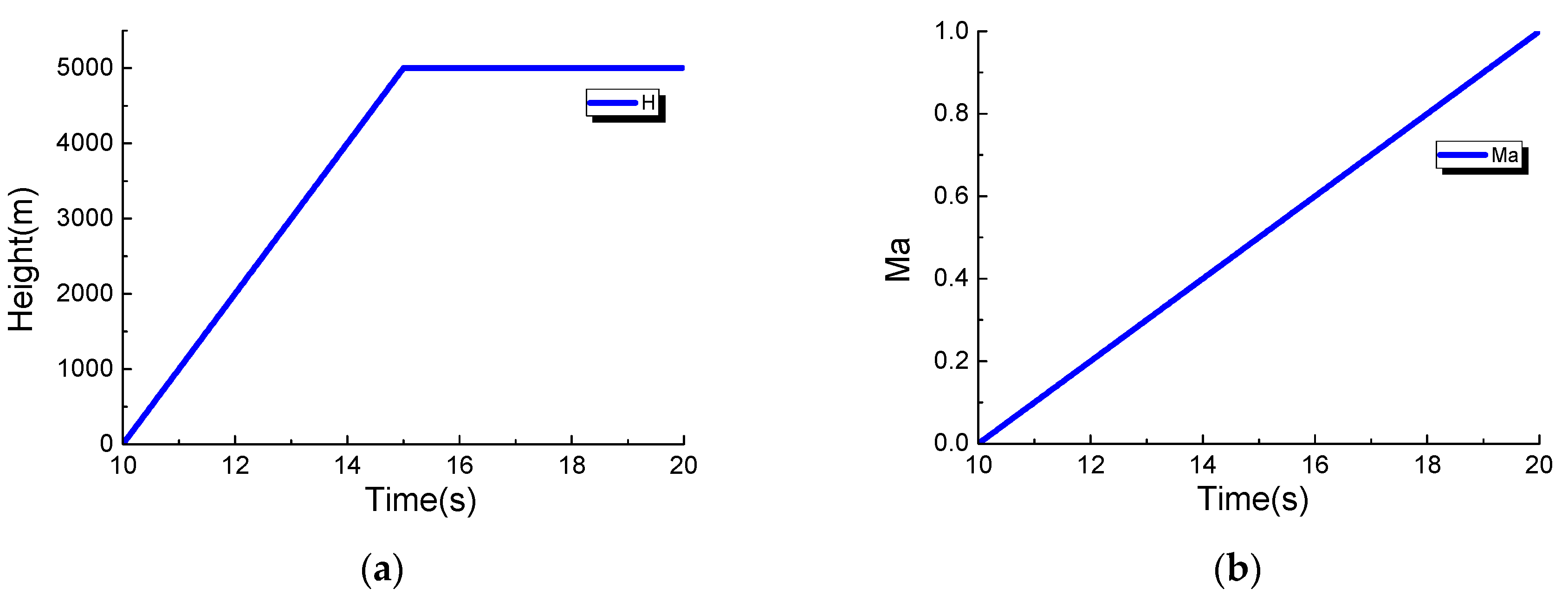
Furthermore, transient performance tests of the proposed methodology are implemented in the flight envelope, and control variables fuel flow Wf and nozzle area A8 change along flight operation H and Ma. The engine starts from the ground point H = 0, Ma = 0, climbs to high altitude (H = 5000, Ma = 1), and the whole operation lasts 10 s. It runs at the full power operation using closed-loop control strategy of spool speed. Figure 7 shows the change route of four input variables during transient process in the flight envelope. The deviation quantities related to each fault scenario are initially added into health parameters as well as that of the ground operation.
The observation sequence length of training data is 100, and there are 1300 samples in total used for 13 fault cases. The average training time of fault cases by HMM, KPCA-HMM and IRKPCA-HMM are 26.75 s, 22.43 s and 17.75 s, respectively. The training time of the IRKPCA-HMM is the least among the examined algorithms. The indices of LL* and Nc by the examined HMMs at CN = 0 in the transient process is given in Table 12.
From Table 12, the indices of LL* and Nc by IRKPCA-HMM at CN = 0 are the largest ones in the most fault cases in the flight envelope. The topological parameters of three HMMs and average performance indices in all fault scenarios at CN = 0, CN = 807, CN = 1558 are reported in Table 12. The fault feature number and optimal hidden state number of basic HMM are clearly larger than the others. It indicates that the topological structure of the HMMs is clearly simplified after feature extraction by the KPCA and IRKPCA, and it is positive for reducing computational time of gas-path fault diagnosis.
5. Conclusions
This paper develops a systematic approach to fault feature extraction and pattern recognition, which leads to an improved data-driven fault diagnosis method. The novelty of this methodology lies in the development of IRKPCA and HMM in combination to facilitate gas-path fault diagnosis for turbofan engines. The reduced samples from IRKPCA in feature space decrease the measurement dimension while the principal information of fault feature is retained. The IRKPCA is evaluated using general benchmark datasets, and the results reveal that IRKPCA is superior to plain KPCA regarding discriminative power, sparsity and reduced dimension time. The simplified observation sequence by IRKPCA is utilized by HMM to develop an IRKPCA-HMM algorithm. The goal of this methodology is to increase gas-path fault diagnostic accuracy and relieve computational effort both in steady and transient behaviors. The proposed methodology is evaluated in the scenarios of gas-path abrupt fault mixed with gradual degradation in the flight envelope, and test data are generated from a dual-spool turbofan engine model. The stochastic diagnostic modeling framework is presented and numerically assessed by several performance indices. The advantage of the proposed methodology is that it does not only produce more reliable results but also consumes less computational efforts of fault diagnosis.
This research establishes a new direction in data-driven fault diagnosis by proposing IRKPCA-HMM technique that is specifically beneficial to gas-path stochastic fault diagnosis for turbofan engine applications. The methodology developed in this study is not only limited to turbofan engine, but also extended to other types of gas turbine engine. There are some important topics for further study related to this work. First, further studies can be carried out to investigate various kernels used to map the measurement space to feature space. Second, extensions of the cases that have more than one gas-path abrupt fault, added to gradual degradation and the tests of semi-physical hardware in the loop, are worthy of future exploration.
Author Contributions
F.L. and J.H. contributed in developing the ideas of this research, J.J. and X.Q. performed this research. All of the authors were involved in preparing this manuscript.
Funding
We are grateful for the financial support of the Fundamental Research Funds for the Central Universities (No. NS2015027).
Acknowledgments
Gratitude is extended to Viliam Makis for useful advices and to China Scholarship Council for supporting the first author to carry out collaborative research in the Department of Mechanical and Industrial Engineering at the University of Toronto.
Conflicts of Interest
The authors declare no conflict of interest. The founding sponsors had no role in the design of the study; in the collection, analyses, or interpretation of data; in the writing of the manuscript, and in the decision to publish the results.
Nomenclature
| PCA | Principal component analysis |
| HMM | Hidden Markov model |
| HPC | High-pressure compressor |
| LPT | Low-pressure turbine |
| HPT | High-pressure turbine |
| L1 | Norm-1 |
| L2 | Norm-2 |
| LL | Log-likelihood |
| H | Height |
| Ma | Mach number |
| SW | Flow capacity |
| SE | Efficiency |
| NL | Low-pressure spool speed |
| NH | High-pressure spool speed |
| T22 | Compressor inlet temperature |
| P22 | Compressor inlet Pressure |
| P3 | Compressor outlet pressure |
| T3 | Compressor outlet temperature |
| T43 | low pressure turbine inlet temperature |
| P43 | low pressure turbine inlet pressure |
| P5 | low pressure turbine outlet pressure |
| T6 | mixing chamber inlet temperature |
| Wf | Fuel flow |
| A8 | Nozzle area |
References
- Zaidan, M.A.; Mills, A.R.; Harrison, R.F.; Fleming, P.J. Gas turbine engine prognostics using Bayesian hierarchical models: A variational approach. Mech. Syst. Signal Process. 2016, 70–71, 120–140. [Google Scholar] [CrossRef]
- Li, J.; Fan, D.; Sreeram, V. SFC optimization for aero engine based on hybrid GA-SQP method. Int. J. Turbo Jet-Engines 2013, 30, 383–391. [Google Scholar] [CrossRef]
- Kraft, J.; Sethi, V.; Singh, R. Optimization of aero gas turbine maintenance using advanced simulation and diagnostic methods. J. Eng. Gas Turbines Power 2014, 136, 111601. [Google Scholar] [CrossRef]
- Salahshoor, K.; Kordestani, M.; Khoshro, M.S. Fault detection and diagnosis of an industrial steam turbine using fusion of SVM (support vector machine) and ANFIS (adaptive neuro-fuzzy inference system) classifiers. Energy 2010, 35, 5472–5482. [Google Scholar] [CrossRef]
- Mohammadi, E.; Montazeri-Gh, M. Performance enhancement of global optimization-based gas turbine fault diagnosis systems. J. Propuls. Power 2016, 32, 214–224. [Google Scholar] [CrossRef]
- Lu, F.; Ju, H.; Huang, J. An improved extended Kalman filter with inequality constraints for gas turbine engine health monitoring. Aerosp. Sci. Technol. 2016, 58, 36–47. [Google Scholar] [CrossRef]
- Wen, H.; Zhu, Z.H.; Jin, D.; Hu, H. Model predictive control with output feedback for a deorbiting electrodynamic tether system. J. Guid. Control Dyn. 2016, 39, 2455–2460. [Google Scholar] [CrossRef]
- Tahan, M.; Tsoutsanis, E.; Muhammad, M.; Karim, Z.A.A. Performance-based health monitoring, diagnostics and prognostics for condition-based maintenance of gas turbines: A review. Appl. Energy 2017, 198, 122–144. [Google Scholar] [CrossRef] [Green Version]
- Zhang, S.G.; Guo, Y.Q.; Chen, X.L. Performance evaluation and simulation validation of fault diagnosis system for aircraft engine. J. Propuls. Technol. 2013, 34, 1121–1127. [Google Scholar]
- Yang, C.; Kong, X.X.; Wang, X. Model-based fault diagnosis for performance degradation of turbofan gas path via optimal robust residuals. In Proceedings of the ASME Turbo Expo: Turbine Technical Conference and Exposition, Seoul, South Korea, 13–17 June 2016; Volume 6. [Google Scholar]
- Zhou, D.J.; Yu, Z.Q.; Zhang, H.S.; Weng, S.L. A novel grey prognostic model based on Markov process and grey incidence analysis for energy conversion equipment degradation. Energy 2016, 109, 420–429. [Google Scholar] [CrossRef]
- Zhao, X.F.; Liu, Y.B.; He, X. Diagnosis of gas turbine based on fuzzy matrix and the principle of maximum membership degree. Energy Procedia 2012, 16, 1448–1454. [Google Scholar] [CrossRef]
- Zhong, S.S.; Luo, H.; Lin, L. An improved correlation-based anomaly detection approach for condition monitoring data of industrial equipment. In Proceedings of the IEEE International Conference on Prognostics and Health Management (ICPHM), Ottawa, ON, Canada, 20–22 June 2016. [Google Scholar]
- Amozegar, M.; Khorasani, K. An ensemble of dynamic neural network identifiers for fault detection and isolation of gas turbine engines. Neural Netw. 2016, 76, 106–121. [Google Scholar] [CrossRef] [PubMed]
- Bartolini, C.M.; Caresana, F.; Comodi, G.; Pelagalli, L.; Renzi, M.; Vagni, S. Application of artificial neural networks to micro gas turbines. Energy Convers. Manag. 2011, 52, 781–788. [Google Scholar] [CrossRef]
- Owsley, L.M.D.; Atlas, L.E.; Bernard, G.D. Self-organizing feature maps and hidden Markov models for machine-tool monitoring. IEEE Trans. Signal Process. 1997, 45, 2787–2798. [Google Scholar] [CrossRef]
- Boutros, T.; Liang, M. Detection and diagnosis of bearing and cutting tool faults using hidden Markov models. Mech. Syst. Signal Process. 2011, 25, 2102–2124. [Google Scholar] [CrossRef]
- Soualhi, A.; Clerc, G. Hidden Markov models for the prediction of impending faults. IEEE Trans. Ind. Electron. 2016, 63, 3271–3281. [Google Scholar] [CrossRef]
- Shi, S.B.; Li, G.N.; Chen, H.X.; Hu, Y.P.; Wang, X.Y.; Guo, Y.B.; Sun, S.B. An efficient VRF system fault diagnosis strategy for refrigerant charge amount based on PCA and dual neural network model. Appl. Therm. Eng. 2018, 129, 1252–1262. [Google Scholar] [CrossRef]
- Ni, J.J.; Zhang, C.B.; Yang, S.X. An adaptive approach based on KPCA and SVM for real-time fault diagnosis of HVCBs. IEEE Trans. Power Deliv. 2011, 26, 1960–1971. [Google Scholar] [CrossRef]
- Taouali, O.; Jaffel, I.; Lahdhiri, H.; Harkat, M.F.; Messaoud, H. New fault detection method based on reduced kernel principal component analysis (RKPCA). Int. J. Adv. Manuf. Technol. 2015, 85, 1547–1562. [Google Scholar] [CrossRef]
- Lu, F.; Wang, Y.F.; Huang, J.Q.; Huang, Y.H. Gas turbine transient performance tracking using data fusion based on an adaptive particle filter. Energies 2015, 8, 13911–13927. [Google Scholar] [CrossRef]
- You, C.X.; Huang, J.Q.; Lu, F. Recursive reduced kernel based extreme learning machine for aero-engine fault pattern recognition. Neurocomputing 2016, 214, 1038–1045. [Google Scholar] [CrossRef]
- Kasun, L.L.C.; Yang, Y.; Huang, G.B.; Zhang, Z.Y. Dimension reduction with extreme learning machine. IEEE Trans. Image Process. 2016, 25, 3906–3918. [Google Scholar] [CrossRef] [PubMed]
- Demiriz, A.; Bennett, K.P.; Shawe-Taylor, J. Linear Programming Boosting via Column Generation. Mach. Learn. 2002, 46, 225–254. [Google Scholar] [CrossRef] [Green Version]
- Khaleghei, A.; Makis, V. Model parameter estimation and residual life prediction for a partially observable failing system. Nav. Res. Logist. 2015, 62, 190–205. [Google Scholar] [CrossRef]
- Yan, X.; Jia, M.P. Compound fault diagnosis of rotating machinery based on OVMD and a 1.5-dimension envelope spectrum. Meas. Sci. Technol. 2016, 27, 075002. [Google Scholar] [CrossRef]
- Windmann, S.; Jungbluth, F.; Niggemann, O. A HMM-based fault detection method for piecewise stationary industrial processes. In Proceedings of the IEEE 20th Conference on Emerging Technologies & Factory Automation, Luxembourg, 8–11 September 2015. [Google Scholar]
- Veprek, P.; Bardley, A.B. An improved algorithm for vector quantizer design. IEEE Signal Process. Lett. 2000, 7, 250–252. [Google Scholar] [CrossRef]
- Lu, F.; Huang, J.Q.; Lv, Y.Q. Gas path health monitoring for a turbofan engine based on a nonlinear filtering approach. Energies 2013, 6, 492–523. [Google Scholar] [CrossRef]
- Chaibakhsh, A.; Amirkhani, S. A simulation model for transient behaviour of heavy-duty gas turbines. Appl. Therm. Eng. 2018, 132, 115–127. [Google Scholar] [CrossRef]
- Qi, Y.W.; Bao, W.; Chang, J.T. State-based switching control strategy with application to aeroengine safety protection. J. Aerosp. Eng. 2015, 28, 04014076. [Google Scholar] [CrossRef]
- Lu, F.; Jiang, J.P.; Huang, J.Q.; Qiu, X.J. Dual reduced kernel extreme learning machine for aero-engine fault diagnosis. Aerosp. Sci. Technol. 2017, 71, 742–750. [Google Scholar] [CrossRef]
- Wang, C.; Li, Y.G.; Yang, B.Y. Transient performance simulation of aircraft engine integrated with fuel and control systems. Appl. Therm. Eng. 2017, 114, 1029–1037. [Google Scholar] [CrossRef]
- Aretakis, N.; Roumeliotis, I.; Alexiou, A.; Romesis, C.; Mathioudakis, K. Turbofan engine health assessment from flight data. J. Eng. Gas Turbines Power 2015, 137, 041203. [Google Scholar] [CrossRef]
- Borguet, S.; Leonerd, O. Comparison of adaptive filters for gas turbine performance monitoring. J. Comput. Appl. Math. 2010, 234, 2201–2212. [Google Scholar] [CrossRef]
- Camci, F.; Chinnam, R.B. Health-state estimation and prognostics in machining processes. IEEE Trans. Autom. Sci. Eng. 2010, 7, 581–596. [Google Scholar] [CrossRef] [Green Version]
Figure 1.
Extraction effect on Iris dataset and wine dataset by the IRKPCA.

Figure 2.
The structure of improved IRKPCA-HMM algorithm.
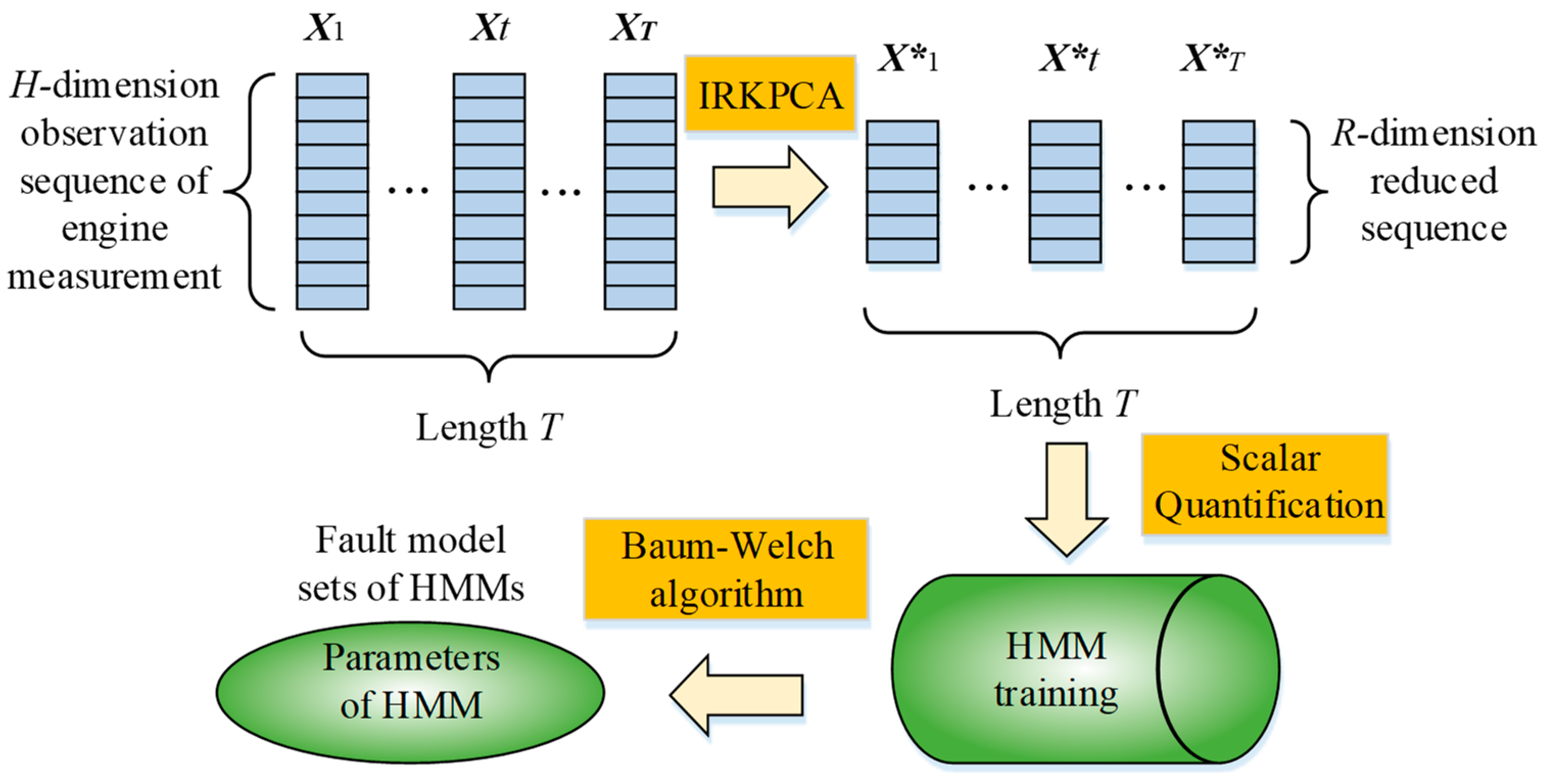
Figure 3.
A dual-spool turbofan engine gas-path component cross-section diagram.
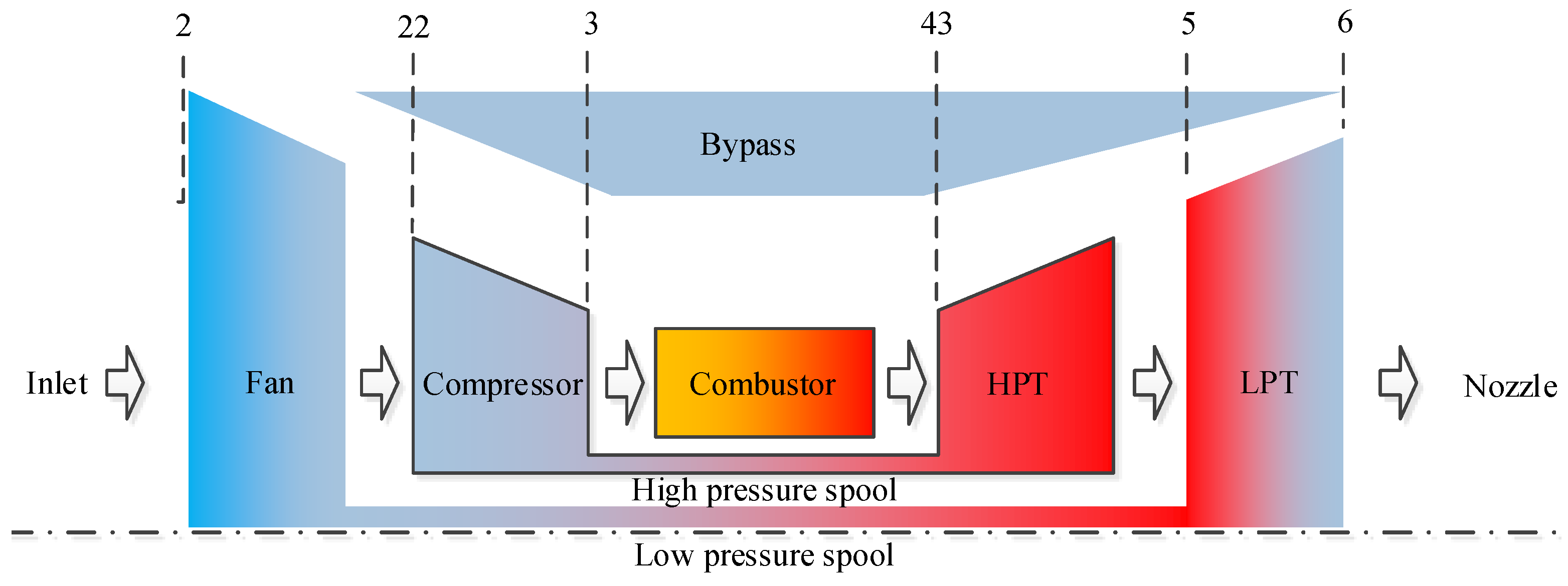
Figure 4.
Gas-path fault diagnosis framework for turbofan engine based on IRKPCA-HMM.

Figure 5.
The effect comparison of gas-path fault feature extraction using IRKPCA.
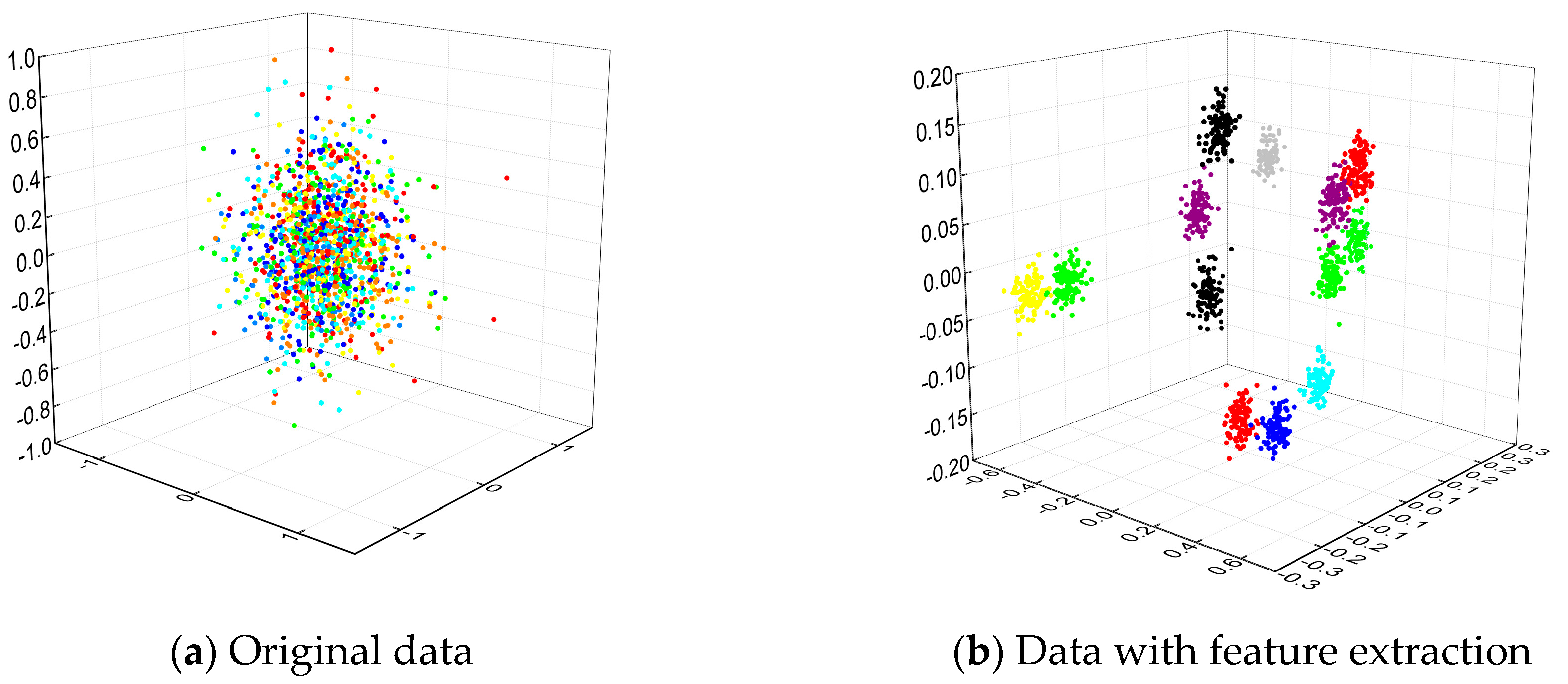
Figure 6.
Variations of fuel flow and nozzle area of the engine in the transient process.
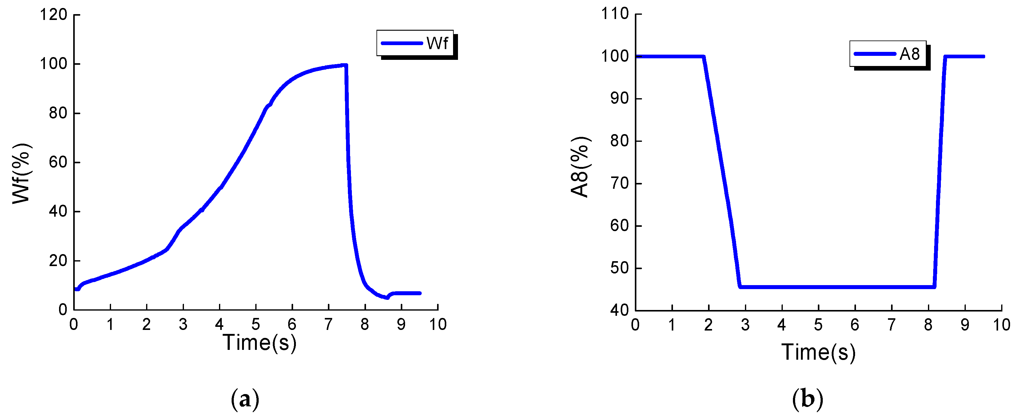
Figure 7.
The change route of engine input variables in the transient process in flight envelope.


Table 1.
Specification of these benchmark datasets.
| Datasets | Feature | Class | SN |
|---|---|---|---|
| Iris | 4 | 3 | 150 |
| Wine | 13 | 3 | 178 |
| Glass | 10 | 6 | 214 |
| E.coli | 7 | 5 | 336 |
| Balance | 4 | 3 | 625 |
| Vehicle | 18 | 4 | 846 |
Table 2.
Performance comparisons of basic KPCA and IRKPCA on the benchmark datasets.
| Dataset | Algorithms | Modeling Parameters | Reduced Features | Discriminative Power | L2/L1 | Reduced Time (s) |
|---|---|---|---|---|---|---|
| Iris | KPCA | σ = 210 | 2 | 0.9564 ± 0.0155 | 0.0928 | 0.0372 |
| IRKPCA | σ = 29 ρ = 2−1 | 2 | 0.9600 ± 0.0158 | 0.0945 | 0.0080 | |
| Wine | KPCA | σ = 210 | 10 | 0.8609 ± 0.0335 | 0.0849 | 0.0517 |
| IRKPCA | σ = 210 ρ = 21 | 8 | 0.8621 ± 0.0435 | 0.0851 | 0.0089 | |
| Glass | KPCA | σ = 29 | 7 | 0.6453 ± 0.0290 | 0.0967 | 0.0726 |
| IRKPCA | σ = 210 ρ = 1 | 6 | 0.6438 ± 0.0284 | 0.0974 | 0.0115 | |
| E.coli | KPCA | σ = 27 | 6 | 0.8847 ± 0.0135 | 0.0627 | 0.1069 |
| IRKPCA | σ = 29 ρ = 2−1 | 5 | 0.9117 ± 0.0112 | 0.0717 | 0.0149 | |
| Balance | KPCA | σ = 28 | 4 | 0.8576 ± 0.136 | 0.0512 | 0.5873 |
| IRKPCA | σ = 28 ρ = 1 | 3 | 0.8897 ± 0.130 | 0.0791 | 0.0288 | |
| Vehicle | KPCA | σ = 210 | 8 | 0.7198 ± 0.0128 | 0.0402 | 1.2387 |
| IRKPCA | σ = 29 ρ = 2−1 | 7 | 0.7201 ± 0.0114 | 0.0404 | 0.0645 |
Table 3.
Turbofan engine control variables, health parameters, and measured variables.
| Control Variables | Health Parameters | Measured Outputs |
|---|---|---|
| Wf—Fuel flow | SE1—Fan efficiency indicator | NL—LPC speed |
| A8—Nozzle area | SW1—Fan flow indicator | NH—HPC speed |
| SE2—Compressor efficiency indicator | T22—Compressor inlet temperature | |
| SW2—Compressor flow indicator | P22—Compressor inlet pressure | |
| SE3—HPT efficiency indicator | P3—Compressor outlet pressure | |
| SW3—HPT flow indicator | T3—Compressor outlet temperature | |
| SE4—LPT efficiency indicator | T43—Low pressure turbine inlet temperature | |
| SW4—LPT flow indicator | P43—Low pressure turbine inlet pressure | |
| P5—Low pressure turbine outlet pressure | ||
| T6—Mixer inlet temperature |
Table 4.
Gradual degradation of turbofan engine performance over time.
| CN | SW1 (%) | SE1 (%) | SW2 (%) | SE2 (%) | SW3 (%) | SE3 (%) | SW4 (%) | SE4 (%) |
|---|---|---|---|---|---|---|---|---|
| 0 | 0 | 0 | 0 | 0 | 0 | 0 | 0 | 0 |
| 807 | −0.4125 | −0.2704 | −0.5190 | −0.4593 | 0.5212 | −0.8142 | 0.0632 | −0.0896 |
| 1558 | −0.7886 | −0.5316 | −1.1219 | −0.9689 | 0.9032 | −1.3919 | 0.1151 | −0.1796 |
Table 5.
Turbofan engine gas-path performance fault cases.
| Scenario | Variations of Health Parameter | Faulty Component |
|---|---|---|
| I | SE1 −1% | Fan |
| II | SE1 −0.5% and SW1 −1% | |
| III | SE2 −1% | Compressor |
| IV | SW2 −1% | |
| V | SE2 −0.7% and SW2 −1% | |
| VI | SE3 −1% | HPT |
| VII | SW3 +1% | |
| VIII | SE3 −1% and SW3 −1% | |
| IX | SE4 −1% | LPT |
| X | SW4 −1% | |
| XI | SE4 −0.4% and SW4 −1% | |
| XII | SE4 −0.6% and SW4 +1% |
Table 6.
LL* and Nc by three HMMs in the steady process at CN = 1558.
| Fault Scenarios | HMM | KPCA-HMM | IRKPCA-HMM | |||
|---|---|---|---|---|---|---|
| LL* | Nc | LL* | Nc | LL* | Nc | |
| I | −1195.13 | 9 | −398.65 | 10 | −302.47 | 10 |
| II | −1433.33 | 8 | −453.51 | 8 | −362.97 | 8 |
| III | −1154.37 | 10 | −446.14 | 8 | −429.36 | 9 |
| IV | −1371.25 | 8 | −503.75 | 9 | −399.32 | 9 |
| V | −1226.52 | 10 | −415.89 | 10 | −415.88 | 10 |
| VI | −1360.83 | 9 | −404.67 | 9 | −258.15 | 9 |
| VII | −1203.93 | 8 | −512.18 | 8 | −420.53 | 9 |
| VIII | −1358.67 | 7 | −530.84 | 9 | −312.82 | 8 |
| IX | −1217.61 | 10 | −454.51 | 10 | −299.79 | 10 |
| X | −1367.24 | 9 | −369.51 | 9 | −362.25 | 10 |
| XI | −1274.02 | 9 | −419.78 | 10 | −439.94 | 8 |
| XII | −1150.72 | 8 | −386.98 | 9 | −250.36 | 9 |
| XIII | −1269.47 | 9 | −420.05 | 8 | −320.03 | 8 |
Table 7.
Parameters of IRKPCA-HMM at CN = 0 in fault mode 1.
| Transition Matrix | Confusion Matrix | ||||||||||||||
|---|---|---|---|---|---|---|---|---|---|---|---|---|---|---|---|
| 0.75 | 0.25 | 0 | 0 | 0 | 0 | 0.044 | 0.042 | 0.037 | 0.039 | 0.047 | 0.231 | 0.242 | 0.252 | 0.040 | 0.020 |
| 0 | 0.69 | 0.31 | 0 | 0 | 0 | 0.060 | 0.077 | 0.064 | 0.064 | 0.057 | 0 | 0 | 0.003 | 0.366 | 0.304 |
| 0 | 0 | 0.74 | 0.26 | 0 | 0 | 0.094 | 0.085 | 0.080 | 0.307 | 0.373 | 0.058 | 0 | 0 | 0 | 0 |
| 0 | 0 | 0 | 0.84 | 0.16 | 0 | 0.446 | 0.400 | 0.154 | 0 | 0 | 0 | 0 | 0 | 0 | 0 |
| 0 | 0 | 0 | 0 | 0.46 | 0.54 | 0 | 0 | 1 | 0 | 0 | 0 | 0 | 0 | 0 | 0 |
| 0 | 0 | 0 | 0 | 0 | 1 | 0 | 0 | 0.379 | 0.621 | 0 | 0 | 0 | 0 | 0 | 0 |
Table 8.
Fault diagnosis comparisons of the HMMs in the ground steady process.
| CN | Algorithms | Reduced Features | Hidden States | Acc ± Std | ttest |
|---|---|---|---|---|---|
| 0 | HMM | 10 | 5 | 0.9108 ± 0.0124 | 0.2958 |
| KPCA-HMM | 6 | 4 | 0.9305 ± 0.0063 | 0.4237 | |
| IRKPCA-HMM | 6 | 4 | 0.9226 ± 0.0044 | 0.2654 | |
| 807 | HMM | 10 | 5 | 0.9054 ± 0.0103 | 0.3096 |
| KPCA-HMM | 6 | 3 | 0.9208 ± 0.0072 | 0.4045 | |
| IRKPCA-HMM | 6 | 4 | 0.9174 ± 0.0053 | 0.2596 | |
| 1558 | HMM | 10 | 5 | 0.8785 ± 0.0125 | 0.3013 |
| KPCA-HMM | 6 | 4 | 0.8953 ± 0.0082 | 0.4109 | |
| IRKPCA-HMM | 6 | 3 | 0.8907 ± 0.0068 | 0.2432 |
Table 9.
Comparisons of fault diagnosis methods in high altitude steady operation.
| CN | Algorithms | Reduced Features | Hidden States | Acc ± Std | ttest |
|---|---|---|---|---|---|
| 0 | HMM | 10 | 5 | 0.8916 ± 0.0103 | 0.2809 |
| KPCA-HMM | 6 | 3 | 0.9012 ± 0.0070 | 0.4254 | |
| IRKPCA-HMM | 6 | 3 | 0.8983 ± 0.0053 | 0.2543 | |
| 807 | HMM | 10 | 5 | 0.8795 ± 0.0114 | 0.3025 |
| KPCA-HMM | 6 | 4 | 0.8902 ± 0.0065 | 0.4181 | |
| IRKPCA-HMM | 6 | 3 | 0.8883 ± 0.0058 | 0.2496 | |
| 1558 | HMM | 10 | 5 | 0.8501 ± 0.0130 | 0.2957 |
| KPCA-HMM | 6 | 4 | 0.8676 ± 0.0068 | 0.4316 | |
| IRKPCA-HMM | 6 | 3 | 0.8602 ± 0.0049 | 0.2601 |
Table 10.
LL* and Nc by three HMMs at CN = 0 in the transient process of ground operation.
| Fault Scenarios | HMM | KPCA-HMM | IRKPCA-HMM | |||
|---|---|---|---|---|---|---|
| LL* | Nc | LL* | Nc | LL* | Nc | |
| I | −1809.88 | 10 | −926.16 | 10 | −725.03 | 10 |
| II | −1654.79 | 10 | −759.55 | 10 | −566.62 | 9 |
| III | −1804.08 | 8 | −760.09 | 10 | −658.05 | 9 |
| IV | −1636.12 | 6 | −893.39 | 8 | −865.88 | 10 |
| V | −1804.72 | 10 | −748.01 | 10 | −639.46 | 10 |
| VI | −1707.47 | 7 | −824.51 | 8 | −723.78 | 8 |
| VII | −1821.22 | 7 | −780.72 | 9 | −641.11 | 9 |
| VIII | −1676.86 | 8 | −710.99 | 10 | −711.86 | 10 |
| IX | −1831.40 | 9 | −704.30 | 10 | −600.94 | 10 |
| X | −1685.29 | 9 | −713.12 | 10 | −766.83 | 10 |
| XI | −1696.52 | 6 | −840.63 | 9 | −686.89 | 9 |
| XII | −1861.67 | 10 | −795.27 | 10 | −709.48 | 10 |
| XIII | −1685.33 | 4 | −596.59 | 9 | −470.51 | 9 |
Table 11.
Fault diagnosis result comparisons in the transient process of ground operation over time.
Table 11.
Fault diagnosis result comparisons in the transient process of ground operation over time.
| CN | Algorithms | Reduced Features | Hidden States | Acc ± Std | ttest |
|---|---|---|---|---|---|
| 0 | HMM | 10 | 6 | 0.7931 ± 0.0053 | 0.2938 |
| KPCA-HMM | 4 | 4 | 0.9474 ± 0.0036 | 0.3992 | |
| IRKPCA-HMM | 4 | 3 | 0.9446 ± 0.0033 | 0.1948 | |
| 807 | HMM | 10 | 5 | 0.8157 ± 0.0047 | 0.2824 |
| KPCA-HMM | 4 | 3 | 0.9402 ± 0.0035 | 0.3319 | |
| IRKPCA-HMM | 4 | 4 | 0.9362 ± 0.0028 | 0.1891 | |
| 1558 | HMM | 10 | 5 | 0.8023 ± 0.0057 | 0.2602 |
| KPCA-HMM | 4 | 4 | 0.9386 ± 0.0041 | 0.3707 | |
| IRKPCA-HMM | 4 | 4 | 0.9306 ± 0.0037 | 0.2030 |
Table 12.
LL* and Nc by three HMMs during dynamic process in the flight envelope at CN = 0.
| Fault Scenarios | HMM | KPCA-HMM | IRKPCA-HMM | |||
|---|---|---|---|---|---|---|
| LL* | Nc | LL* | Nc | LL* | Nc | |
| I | −2013.02 | 8 | −1021.62 | 10 | −925.03 | 10 |
| II | −1895.17 | 7 | −872.45 | 9 | −716.43 | 9 |
| III | −1974.28 | 6 | −853.12 | 9 | −658.52 | 9 |
| IV | −1862.29 | 7 | −983.43 | 7 | −865.16 | 8 |
| V | −2084.42 | 9 | −855.09 | 9 | −709.75 | 9 |
| VI | −1906.54 | 6 | −934.16 | 8 | −815.87 | 8 |
| VII | −2021.33 | 6 | −870.39 | 9 | −734.27 | 8 |
| VIII | −1892.18 | 7 | −819.09 | 9 | −756.13 | 10 |
| IX | −2011.04 | 5 | −844.60 | 10 | −694.26 | 9 |
| X | −1889.25 | 6 | −793.25 | 7 | −706.83 | 6 |
| XI | −1906.27 | 7 | −841.42 | 9 | −741.14 | 9 |
| XII | −2056.71 | 8 | −896.71 | 8 | −811.73 | 8 |
| XIII | −1892.35 | 4 | −696.87 | 6 | −624.29 | 6 |
© 2018 by the authors. Licensee MDPI, Basel, Switzerland. This article is an open access article distributed under the terms and conditions of the Creative Commons Attribution (CC BY) license (http://creativecommons.org/licenses/by/4.0/).
Share and Cite
MDPI and ACS Style
Lu, F.; Jiang, J.; Huang, J.; Qiu, X. An Iterative Reduced KPCA Hidden Markov Model for Gas Turbine Performance Fault Diagnosis. Energies 2018, 11, 1807. https://doi.org/10.3390/en11071807
AMA Style
Lu F, Jiang J, Huang J, Qiu X. An Iterative Reduced KPCA Hidden Markov Model for Gas Turbine Performance Fault Diagnosis. Energies. 2018; 11(7):1807. https://doi.org/10.3390/en11071807
Chicago/Turabian StyleLu, Feng, Jipeng Jiang, Jinquan Huang, and Xiaojie Qiu. 2018. "An Iterative Reduced KPCA Hidden Markov Model for Gas Turbine Performance Fault Diagnosis" Energies 11, no. 7: 1807. https://doi.org/10.3390/en11071807
Note that from the first issue of 2016, this journal uses article numbers instead of page numbers. See further details here.