A Robust Day-Ahead Electricity Market Clearing Model Considering Wind Power Penetration

Abstract

With the development and grid-connection of renewable energy sources such as wind power, there are more and more uncertainties in power systems, and large-scale wind power has brought many challenges to the security and stability the systems. These uncertainties have to be eliminated by means of upward or downward regulations of conventional generators and charging/discharging services of energy storage devices. Based on the analysis of the influence of wind power uncertainties on the day-ahead electricity market, this article proposes a robust clearing model for the day-ahead electricity market considering the wind power penetration, which can help to complete the dispatch of power system. Compared with the traditional models, the proposed model is a multi-objective model, which considers both the lowest operating cost and the least wind power curtailment of power system. Moreover, the obtained dual multipliers $\mathsf{\lambda }$ corresponding to the power balance constraints reflect the marginal cost of the power production in a certain period, that is, the locational marginal price (LMP), which can be used as the clearing prices. This robust market clearing model takes into consideration the economic and reliability of the system operation and accommodates as much renewable energy as possible. The simulation of three wind power producers was implemented on the IEEE 30-bus test system, which verified the rationality of the proposed approaches.

1. Introduction

In recent years, with the continuous development of China’s wind power industry, the total installed capacity of wind power has increased. Wind power is leading the transition from fossil energy to clean energy globally. By the end of 2015, China’s cumulative wind power installed capacity reached to 145,104 MW, making China the largest wind power installation country with 33.6% of the global share. China is a major country in both of the wind power installed capacity and wind power curtailment. In the first half of 2015, the average rate of wind power curtailment in China had reached 15.2%, resulting in direct economic losses of more than 16 billion yuan. Hence, it is urgent to solve the wind power curtailment problem caused by large-scale wind power penetration in the power system. Traditional power generation dispatch plans are based on the consideration of controllable power output and predictable load characteristics [1,2,3]. After an uncontrolled power supply like wind power is introduced, the research points of optimized dispatch are mainly reflected in two aspects: the first is how to establish a more accurate forecasting model of wind power output [4,5,6]; the second is how to make conventional generators leave reasonable reserve capacity in response to uncertainties of wind power producers [7,8,9]. Traditional reserve capacity is obtained from the deterministic calculation method, that is, the fixed proportion of system load and the largest single capacity in the system. However, due to the stochastic fluctuation characteristics of wind power, the traditional method cannot meet the requirements of the economics and reliability of the system. Therefore, it is necessary to research the day-ahead market clearing model with the large-scale wind power penetration, which can lay a foundation for the gradual promotion of China’s spot electricity market.

The spot market refers to the market that focuses on short-term and instant electricity transactions, which is an important part of the electric power trading mechanism. Firstly, affected by the power system, it is usually in the day-ahead stage that the ISO can accurately confirm the operation and starting conditions of each generating unit, and analyze the network structure of power systems. Therefore, establishing the spot market at this time can make the result of the transaction be more in line with the actual situation, which can really help to ensure the safe and stable operation of the power grid. Secondly, through the competition of the spot market, the daily peak-to-valley electricity price, even the real-time electricity price signal, can accurately reflect the real electrical market supply and demand in different times. Thirdly, the spot market can guide the power generators to meet the requirement of electric system peak regulation initiatively by the real-time electricity price signals, and lay a mechanism for the implementation of demand side response. In addition, it can also optimize all the resources in the power grid, so as to effectively promote renewable energy accommodation and reduce the wind power curtailment. Finally, the price signal generated by the spot market is produced by the sufficient competition of all the market participants, which can provide an effective quantitative reference for optimizing resource allocation, planning investment, medium and long-term power trading and power financial market. Besides, the price signal also helps to further stabilize the medium and long term market, and achieve the agreement between the medium and long-term transactions and the real time operation of the power system. The convergence and coordination between the medium and long-term markets and spot transactions help maintain market stability and avoid price fluctuations [10,11,12].

The day-head market is the main trading platform in the spot markets, using “one day” as a suitable advanced time to organize the market, in which the market participants can more accurately predict their own power generation capacity or demand for electricity, so as to form a trading plan which is adaptive and executable to the operation of the power system. However, due to the integration of wind power into the power system, it will make the market supply side uncertain, increasing the decision-making difficulty of the Independent System Operator (ISO). The clearing of day-ahead market is based on the reasonable dispatch made by ISO, so the ISO must take into account the uncertainty of wind power output characteristics when making day-ahead clearing trading plan. Reasonable dispatch means wind power should be accommodated as much as possible in the dispatch, and the conventional generator should leave enough reserve capacity for the uncertainty of wind power. In the market environment, the user transaction settlement mode can be divided into regional marginal electricity price model and locational marginal price model. Compared with the regional marginal price model, the locational marginal price model can effectively use the Optimal Power Flow (OPF) technology to deal with network congestion, so it is widely used. In this paper, the locational marginal price will be used for day-ahead market clearing. ISO, in the dispatch process, will generate a reasonable price, that is, the locational marginal price [13,14].

As for the problem of the power system dispatch caused by the error of wind power output prediction, there are two main kinds of solutions in the existing literature: stochastic optimization methods and robust optimization methods. Stochastic optimization methods are more effective in dealing with the optimization problem with uncertain factors, and how to accurately describe the uncertainty of wind power in the power system is the key to solve the problem of economic dispatch. Stochastic optimization methods mainly describe the uncertainty by a stochastic variable, mainly including chance constrained method and conditional value at risk (CVaR) method [15]. The opportunity-constrained method assumes that the prediction error of wind power or wind power output is subject to a particular type distribution, so as to establish a stochastic programming model that satisfies a certain probability level either by the Weibull distribution of the long-term distribution characterizing wind speed or by the normal distribution [16] and $\beta$ distribution [17] characterizing wind power prediction errors. However, the opportunity constraint is not convex in mathematics, resulting that it is difficult to obtain the overall optimal solution, and the solution obtained by the intelligent algorithm cannot get the definite solutions [18]. By contrast, CVaR introduces a convex function in the modeling process, which can effectively obtain the overall optimal solution [19]. But this kind of solution needs to use Monte Carlo sampling linearization to produce a large number of discrete sample points, resulting in huge computational complexity. In the reference [20], after considering the wake effect, the probability distribution of wind speed was converted into the probabilistic analytic model of the active output of wind power producer, and the dynamic economic dispatch model of power system was established based on wind power cost. The reference [21] forecasted wind speed by probability density function and employed the scenario method to solve the dispatch problem of power system with wind power. In the reference [22], a single period of power system pricing model was established based on the multiple scenarios stochastic programming (MSSP) method considering wind power outputs, finding that the stochastic optimization method often requires a large number of stochastic scenarios in order to ensure the accuracy of the calculation, resulting that the variables are numerous and all have high dimensions. According to the existing method, when solving this problem, stochastic optimization methods will result in huge computation and low computational efficiency [23], which makes it more difficult to meet the practical demands of large scale wind power on-grid.

Robust optimization is an uncertainty decision making method based on interval disturbance information, whose goal is to achieve optimal decisions in the worst conditions of uncertain parameters, so robust optimization is usually called the maximum minimum decision problem [24,25]. Because the robust optimization method has advantages of not requiring the exact probability distribution information of uncertain parameters, quick calculation and suitable for solving large-scale system problems, it has a wide application prospects in power system dispatching problems. According to the relationship between time and space in the wind power producers, the dynamic uncertainty set was constructed in [26], which coupled the perturbation implementation condition of the previous period with the uncertainty set of the current stage, so as to form an adaptive multi period dynamic economic dispatch robust optimization model. This robust optimization model improves the operational efficiency and reliability of decision-making compared with the static economic dispatch. In addition, Xie et al. [27] adopted the advanced dispatching robust optimization model to verify the advantage of the space-time-related wind power forecasting model in improving the utilization of wind power and reducing the total operating cost of the system, and shows that, in the robust optimization model considering wind power fluctuation, the improvement of wind power output prediction accuracy plays an important role in narrowing the range of uncertain collections and controlling the degree of conservativeness in decision making. It is important to note that there is a mutual exclusion relationship between the ability of the system to accept the power disturbance and the economics of the dispatching result. In order to reflect the influence of the two factors on the dispatching results, Li et al. [28] took the maximal upper limit of wind power output and the minimal power generation cost as the optimization objectives to establish robust interval dispatch model. To further clarify the master-slave sequence of safety objectives and economic objectives, Li et al. [29] constructed a real-time dispatching model with two-layer objectives, which formed a two-layer optimization problem. The first layer quantifies the maximum disturbance acceptance ability of the system. On this basis, the second-layer optimization can obtain the most economical dispatch decision results under the condition of maintaining the given disturbance acceptance ability. However, robust optimization also has some shortcomings, that is, the result of the solution is too conservative. In [30], in order to make up the issue that the robust dispatch model result is too conservative, a robust interval dispatch model based on a certain confidence level for wind power output was established, which transformed the problem into single-layer nonlinear programming problem and solved it by Internal Point Method. In [31], the cost function in the objective function was divided into two parts, one part corresponded to the expected cost under the action of stochastic optimization, and the other part corresponded to the worst condition cost which is introduced by the robust optimization method. By assigning the weight coefficient for the two parts, the two optimization methods were unified into one model. By selecting different weight coefficient, the ISO can adjust the conservatism of the unit combination model. However, the influence of power flow constraint on the dispatch results is less considered in the dispatch of power system. In addition, when using the robust optimization method to solve the problem of economic dispatch, the curtailment of wind power is not considered. Wind power, as a clean energy source with low operating costs, should avoid over-curtail, so as to maintain the economic efficiency of the power system operation.

Compared with the method of stochastic optimization, which is widely used in uncertain programming problems, robust optimization has the following characteristics: (1) the decision-making of robust optimization model focuses on the boundary conditions of uncertain parameters, and does not need to know the form of accurate probability distributions. (2) Generally speaking, the robust optimization model can be solved by transforming into its equivalent model, and the scale of the solution is relatively small compared with the stochastic optimization method. In addition, the decision of robust optimization is carried out on the condition that the uncertain parameter is unknown, and a definite numerical solution can be obtained. The decisive result of the robust optimization is sufficient to deal with all the uncertainties, while the constraint of the model is satisfied when the uncertain parameters are taken in a predetermined set of uncertainty sets. Therefore, the effective solution of the robust optimization model is a set of numerical solutions ensuring that all constraints are feasible when the model parameters are arbitrarily taken in the uncertainty set.

On the basis of the above discussion, the robust optimization method is applied to analyze how to carry out the dispatch of the day-ahead market and establish the clearing mechanism in the power system with large-scale wind power penetrating to the grid. However, in the previous robust model, the result of the day-ahead market clearing is formed on the basis of the direct consideration of the uncertainty of the wind power real time output in the objective function which has the worst impact on the operating cost of the system [26,27,28,29]. In the above robust models, the dispatching results may be too conservative, that is, the operation cost of the day-ahead market is too high. On the whole, according to the previous researches, the contributions of this paper mainly include the following two aspects:

(1) If the objective function only includes the minimum operating cost of the system, it may result in less wind power accommodation, making it difficult to fully utilize the renewable energy. Therefore, in this paper, apart from the system operation cost, we also consider reducing the curtailed of wind power as much as possible, so as to establish a multi-objective function. Furthermore, the influence of the change of the curtailed wind power on the average locational marginal price is further analyzed, and the average locational marginal price increases with the increase of the curtailed wind power.

(2) Based on the theory of robust optimization, this paper proposes an approach to improve the day-ahead market clearing model, which is different from some previous reference [26,27,28,29]. This model considers whether the day-ahead clearing results in the feasible region can leave sufficient reserve capacity for the uncertainty caused by the real time output of wind power in the balance stage, instead of direct consideration of the uncertainty of the wind power producers real time output in the objective function which has the worst impact on the operating cost of the system.

The rest of this paper is organized as follows: Section 2 reports the mathematical expressions of the robust day-ahead market clearing model. Section 3 conducts the simulation and comparisons. Section 4 concludes this paper.

2. Problem Description

2.1. Model Assumptions

The spot electricity market is actually a complex dynamic system in which there is dynamic (direct and indirect) interaction among all participants. When considering the behavior of wind power producer in the electric power market, the market clearing model of the ISO should be modified to adapt to the deviation caused by the uncertainty of real time wind power output. In this section, the robust day-ahead market clearing model are expressed using mathematical language. For the sake of simplicity, without loss of generality, before making any further study, we make some assumptions as listed below:

(1)

In this paper, it is assumed that the issue of security constrains unit-commitment (SCUC) has been solved in advance. Therefore, the unit commitment constraints (i.e., ramping rates, minimum down-times, start-up cost/time) are not considered. Moreover, network loss is ignored.

(2)

The electricity demand is inelastic, and load shedding is not considered.

(3)

Uncertainty is caused only by wind power producers, and the set of uncertainties can be truly predicted by the ISO. The marginal cost of each wind power producer is ignored.

2.2. Uncertainty Set

Real-time wind power output cannot be accurately predicted in the current forecast, so the ISO must pay attention to the uncertainty of wind power output when implementing the day-ahead market clearing. However, ISO can more accurately predict the real-time wind power output interval of a certain wind power producers based on previous real-time wind power output. Assuming that there are $N_W$ wind power producers in a power system, the uncertainty set corresponding to these wind power producers’ real time power output can be modeled as [32]:

$$\begin{array}{ll}u:=& \{\stackrel{⌢}{W}=({\stackrel{⌢}{W}}_{1,t},{\stackrel{⌢}{W}}_{2,t},{\stackrel{⌢}{W}}_{3,t},\dots ,{\stackrel{⌢}{W}}_{j,t},\dots ,{\stackrel{⌢}{W}}_{N_W,t}):\\ & W_{j,t}^{\min }\le {\stackrel{⌢}{W}}_{j,t}\le W_{j,t}^{\max },\forall j,t,{\displaystyle \sum _j\frac{\left|2{\stackrel{⌢}{W}}_{j,t}-(W_{j,t}^{\min }+W_{j,t}^{\max })\right|}{(W_{j,t}^{\max }-W_{j,t}^{\min })}}\le \Lambda , \forall j,t\}\end{array}$$

(1)

where, j is the index for wind power producer in the system; ${\stackrel{⌢}{W}}_{j,t}$ is the actual output of the j-th wind power producer at time t; $W_{j,t}^{\max }$ and $W_{j,t}^{\min }$ are the maximum and minimum output limit of wind power at time t; $\Lambda$ is the robustness factor for controlling the size of the uncertain set and this paper assumes it as an integer.

In the day-ahead market stage, when clearing the market, the ISO does not know the real-time natural output of the wind power producers on the next day. However, with the uncertainty set represented by Equation (1), ISO can always take into account the fluctuation range of real-time natural output uncertainty for each wind power producer on the next day. The result of the day-ahead market clearing needs to leave sufficient reserve capacity for the balance stage, that is, at the balance stage, no matter how the real-time natural output of the wind power producers occurs, it can be accommodated by the system as long as it is in the uncertainty set range. In order to meet this requirement, a robust optimization method can be used to improve the clearing model of the day-ahead market.

2.3. Robust Market Clearing Models

According to Section 2.1, it is assumed that the security constrained unit-commitment problem has been solved exogenously beforehand. Therefore, we propose a robust market clearing model, which is mainly concentrated in the economic dispatch process. The purpose of doing so is to make the power system able to eliminate any wind power deviation caused by wind power output uncertainty within a certain set of uncertainty. Under the optimal robust economic dispatch solution, the ISO can re-dispatch the flexible resources, such as a conventional adjustable generator with fast ramping capability, in order to follow the load when deviations occur. In the base case scenario, the method used to obtain an optimal robust economic dispatch solution is much more conservative than that in the worst scenario. In addition, this robust market clearing model can reasonably generate the prices for power outputs and deviations, which are the by-products of the optimal robust economic dispatch solution.

The mathematical formulation of this robust market clearing model can be described as follows:

$$\underset{P_{i,t},W_{j,t},\forall i,j,t}{\min }{\displaystyle \sum _t^T{\displaystyle \sum _i^{N_G}{C}_i(P_{i,\mathrm{t}})}}+{\displaystyle \sum _t^T{\displaystyle \sum _j^{N_W}{C}_j(W_{j,t})}}$$

(2)

$$\underset{W_{j,t}^{spill},\forall j,t}{\min }{\displaystyle \sum _t^T{\displaystyle \sum _j^{N_W}{W}_{j,t}^{spill}}}$$

(3)

$$\mathrm{s}.\mathrm{t}.{\displaystyle \sum _{i\in {\mathsf{\Phi }}_{G,n}}{P}_{i,t}}+{\displaystyle \sum _{j\in {\mathsf{\Phi }}_{W,n}}{W}_{j,t}}-{\displaystyle \sum _{n\in {\mathsf{\Omega }}_n}{D}_{n,t}}={\displaystyle \sum _{n,r\in {\mathsf{\Omega }}_n}\frac{1}{x_{nr}}}({\theta }_n-{\theta }_r),\forall t,n,r$$

(4)

$$P_i^{\min }\le P_{i,t}\le P_i^{\max },\forall t,i$$

(5)

$$R_{D,i}\mathrm{\Delta }T\le P_{i,t}-P_{i,t-1}\le R_{U,i}\mathrm{\Delta }T,\forall t,i$$

(6)

$$W_j^{\min }\le W_{j,t}\le W_j^{\max },\forall t,j$$

(7)

$$\left|\frac{1}{x_{nr}}({\theta }_{n,t}-{\theta }_{r,t})\right|\le F_{nr}^{\max },\forall n,r,t$$

(8)

$${\theta }_1=0$$

(9)

$$\begin{array}{ll}H:=& \{P_{G,W}=(P_{i,t},W_{j,t}):\\ & \forall \stackrel{⌢}{W}\in u,\exists \mathrm{\Delta }P=(\mathrm{\Delta }{P}_1,\mathrm{\Delta }{P}_2,\dots ,\mathrm{\Delta }{P}_{N_G}),\mathrm{such}\mathrm{that}\\ & {\displaystyle \sum _{i\in {\mathsf{\Phi }}_{G,n}}\mathrm{\Delta }{P}_{i,t}+{\displaystyle \sum _{j\in {\mathsf{\Phi }}_{W,n}}({\stackrel{⌢}{W}}_{j,t}-W_{j,t}-W_{j,t}^{spill})}}={\displaystyle \sum _{n,r\in {\mathsf{\Omega }}_n}\frac{1}{x_{nr}}}({\overline{\theta }}_{n,t}-{\overline{\theta }}_{r,t}),\forall t,n,r\end{array}$$

(10)

$$P_i^{\min }\le P_{i,t}+\mathrm{\Delta }{P}_{i,t}\le P_i^{\max },\forall t,i$$

(11)

$$-r_i^d\le \mathrm{\Delta }{P}_{i,t}\le r_i^u,\forall t,i$$

(12)

$$\left|\frac{1}{x_{nr}}({\overline{\theta }}_{n,t}-{\overline{\theta }}_{r,t})\right|\le F_{nr}^{\max },\forall n,r,t$$

(13)

$$0\le W_{j,t}^{spill}\le W_{jt},\forall t,j\}$$

(14)

where, $N$ is the transmission area; $T$ is the total number of periods; $t$ is index of the number of periods; $N_G$ is the total number of conventional generators; $N_W$ is the total number of wind power producers; ${\mathsf{\Phi }}_{G,n},{\mathsf{\Phi }}_{W,n}$ are the set of conventional generators and wind power producers located at bus n in the regional grid, respectively; ${\mathsf{\Omega }}_n$ is the bus set connected to bus n in the regional grid; $P_{i,t}$ is the dispatch power output of the i-th conventional generator at time t; $W_{j,t}$ is the dispatch output of the j-th wind power at time t; $C_i$ is the operating cost coefficient of the i-th conventional generator; $C_j$ is the operating cost coefficient of the j-th wind power producer; $D_{n,t}$ is the load of the bus n at t time in this area. $P_i^{\max },P_i^{\min }$ and $W_j^{\max },W_j^{\min }$ are the upper and lower limits of the output of the conventional generator i, and wind power producer j, respectively; $R_{U,i},R_{D,i}$ are the ramping-up/down limits of the conventional generator i, respectively; ΔT is the time interval; ${\theta }_{n,t},{\theta }_{r,t}$ denote the phase angle of bus n and bus r at the t time, respectively. $x_{n,r}$ is the reactance of line n to r; $F_{nr}^{max}$ is the maximum transmission power of line n to r; u is the uncertainty set of real-time wind power output; $\mathrm{\Delta }{P}_{i,t}$ is the real-time power re-dispatch incremental result of i-th conventional generator for accommodating uncertainties within u. ${\stackrel{⌢}{W}}_{j,t}$ is the real-time output of the j-th wind power at time t.$W_{j,t}^{spill}$ is the curtailed of the wind power of the j-th wind power at time t; ${\overline{\theta }}_{n,t},{\overline{\theta }}_{r,t}$ denote the phase angle of bus n and bus r at the t time at re-dispatch stage, respectively. $r_i^d,r_i^u$ are the ramping-up/down limits of the conventional generator i for uncertainty, respectively.

Among them, Equation (4) indicates power balance of the system, Equations (5) and (7) show the power limits of conventional generator and wind power producer, respectively, Equation (6) represents the ramping constraint of the conventional generator, and Equation (8) indicates the transmission constraints of all lines in system. In case of wind power deviations, Equation (10) represents power balance of the system in re-dispatch, Equation (11) represents the power limits of conventional generators in re-dispatch, Equation (12) is the constraints for power re-dispatch variables $\mathsf{\Delta }{P}_{i,t}$s, Equation (13) represents the line transmission power flow constraints for the system re-dispatch, and Equation (14) is the constraints for the curtailed wind power.

In the above models, the constraints can be divided into two parts. The first part is composed of Equations (2)–(9), which indicates the basic constraints that must be satisfied in the day-ahead market clearing stage. The second part is composed of Equations (10)–(14), which indicates that the day-ahead market clearing result should be able to meet the constraints of real-time dispatching through reasonable secondary adjustments ($\mathrm{\Delta }P$) in the case of any real-time output of wind power producers ($\forall \stackrel{⌢}{W}\in u$), so as to ensure the basic requirement that the day-ahead market clearing results should leave sufficient reserve capacity for the balance stage. Besides, Equations (10)–(14) can present a robust set reflecting the robustness in the feasible region of the model, which is a prerequisite for ensuring robustness of model decision results.

2.4. Model Reformulation

2.4.1. Multi-Objective Optimization Processing

According to the common calculation method of bi-objective optimization [33], the above two objectives function can be transformed as follows, which can simplify the bi-objective programming problem into a single-object programming problem:

(1)

Solve the single-objective optimization model according to objectives 1 and 2 respectively and calculate the output values corresponding to Equations (2) and (3) under their respective optimal decision plans: $C_{\min }^{*},W_{\min }^{spill*}$.

(2)

Consider that when objective 1 and objective 2 are of equal importance, the weight can be equally distributed between them. Therefore, objective 1 and objective 2 can be converted into the following single objective:

$$\min \{\frac{1}{2}\left|\frac{C_{\min }-C_{\min }^{*}}{C_{\min }^{*}}\right|+\frac{1}{2}\left|\frac{W_{\min }^{spill}-W_{\min }^{spill*}}{W_{\min }^{spill*}}\right|\}$$

(15)

2.4.2. Robust Model

By solving these problems, the obtained optimal economic dispatch results $P_{G,W}$ can immunize to any uncertain wind power output. When uncertainty ${\stackrel{⌢}{W}}_{j,t}$ happens, the deviation caused by ${\stackrel{⌢}{W}}_{j,t}$ can be accommodated by the power re-dispatch ΔP. However, it should be noted that the above model can’t be directly resolved. Similar to [32,34], the above model can be solved by reformulation. For ease of description, the reformulation of Equations (2)–(9), which containing the master problem (MP) and the sub-problem (SP), will first be established as follows:

$$(MP)\underset{P_{i,t},W_{j,t},\forall i,j,t}{\min }{\displaystyle \sum _t^T{\displaystyle \sum _i^{N_G}{C}_i(P_{i,t})}}+{\displaystyle \sum _t^T{\displaystyle \sum _j^{N_W}{C}_j(W_{j,t})}}$$

(16)

$$\underset{W_{j,t}^{spill},\forall j,t}{\min }{\displaystyle \sum _t^T{\displaystyle \sum _j^{N_W}{W}_{j,t}^{spill}}}$$

(17)

s.t. Constraint (4)–(9), (14)

$${\displaystyle \sum _{i\in {\mathsf{\Phi }}_{G,n}}\mathrm{\Delta }{P}_{i,k,t}}+{\displaystyle \sum _{j\in {\mathsf{\Phi }}_{W,n}}({\stackrel{⌢}{W}}_{j,k,t}-W_{j,t}-W_{j,t}^{spill})}={\displaystyle \sum _{n,r\in {\mathsf{\Omega }}_n}\frac{1}{x_{nr}}}({\overline{\theta }}_{n,k,t}-{\overline{\theta }}_{r,k,t}),\forall t,n,r,\forall k\in K$$

(18)

$$P_i^{\min }\le P_{i,t}+\mathrm{\Delta }{P}_{i,k,t}^{}\le P_i^{\max },\forall i,t,\forall k\in K$$

(19)

$$-r_i^{\mathrm{d}}\le \mathrm{\Delta }{P}_{i,k,t}^{}\le r_i^u,\forall i,t,\forall k\in K$$

(20)

$$R_{D,i}\mathrm{\Delta }T\le P_{i,k,t}-P_{i,k,t-1}\le R_{U,i}\mathrm{\Delta }T,\forall t,i,\forall k\in K$$

(21)

$$\left|\frac{1}{x_{nr}}({\overline{\theta }}_{n,k,t}-{\overline{\theta }}_{r,k,t})\right|\le F_{nr}^{\max },\forall n,r,t,\forall k\in K$$

(22)

and:

$$(SP)\mathrm{Z}{\rm Z}=\underset{\stackrel{⌢}{W}\in u}{\max }\underset{s^{+},s^{-},\mathrm{\Delta }P}{\min }{\displaystyle \sum _n^{{\mathsf{\Omega }}_n}{\displaystyle \sum _t^T(s_{n,t}^{+}+s_{n,t}^{-})}}$$

(23)

$$\mathrm{s}.\mathrm{t}.{\displaystyle \sum _{i\in {\mathsf{\Phi }}_{G,n}}\mathrm{\Delta }{P}_{i,t}}+{\displaystyle \sum _{j\in {\mathsf{\Phi }}_{W,n}}({\stackrel{⌢}{W}}_{j,t}-W_{j,t}-W_{j,t}^{spill})}+{\displaystyle \sum _{n\in {\mathsf{\Omega }}_n}(s_{n,t}^{+}-s_{n,t}^{-})={\displaystyle \sum _{n,r\in {\mathsf{\Omega }}_n}\frac{1}{x_{nr}}}}({\overline{{\theta }^{\prime }}}_{n,t}-{\overline{{\theta }^{\prime }}}_{r,t}),\forall t,n,r$$

(24)

$${\theta }_1=0$$

(25)

$$s_{n,t}^{+}\ge 0,\forall n,t$$

(26)

$$s_{n,t}^{-}\ge 0,\forall n,t$$

(27)

(11) and (12)

$$\left|\frac{1}{x_{nr}}({\overline{{\theta }^{\prime }}}_{n,t}-{\overline{{\theta }^{\prime }}}_{r,t})\right|\le F_{nr}^{\max },\forall n,r,t$$

(28)

where, K is the exponent set for uncertainty points $\widehat{W_k}s$ which are dynamically generated in the process of solving sub-problems. k is the index of the worst point for uncertainty (element in K). And $\widehat{W_k}$ is the worst point in the uncertainty set u. According to references [26,28], the objective function in (SP) contains the sum of non-negative slack variables $s_{n,t}^{+}$ and $s_{n,t}^{-}$, and its evaluation is related to the solution related to the solution from (MP). $s_{n,t}^{+}$ and $s_{n,t}^{-}$ can be interpreted as un-followed uncertainties due to system constraints (i.e., generation shedding, etc.). Therefore, the solution to the sub-problem is to find the worst point in the uncertainty set $u$ and get the economic dispatching plan accordingly. The calculation process is as follows [34]:

(1)

$K\leftarrow \varnothing ,k\leftarrow 1,Z\leftarrow +\infty$, define feasibility tolerance $\delta$;

(2)

While $Z\ge \delta$, do the next step;

(3)

Solve the (MP) and obtain optimal $P_{i,t},W_{j,t},\forall i,j,t$;

(4)

Solve the (SP) with $P_{i,t},W_{j,t},\forall i,j,t$, and get solution $\left(Z,\widehat{W_k}\right)$;

(5)

$k\leftarrow k\cup K,k\leftarrow k+1$

(6)

End while.

From the iterative process above, it can be seen that the solution of the model takes into account all the “worst points” in the uncertain set u affecting the smooth progress of dispatching. Therefore, the results of the day-ahead clearing can leave sufficient reserve capacity for the balance stage, thereby reducing the curtailment of wind power.

3. Simulation and Discussion

3.1. System Data

In this section, an IEEE 30-bus test system with three wind power producers and six conventional generators is adopted as an example [35]. Matlab 2014b software (MathWorks, Natick, MA, USA) is used for simulation to verify the rationality and decision-making effectiveness of the proposed method.

The network structure of the IEEE 30-bus system is shown in Figure 1. For the sake of simplicity, it is assumed that the maximum power flow constraints for all transmission lines are 30 MW. In addition, the relevant physical and economic parameters of conventional generators are shown in

Table 1. Parameters of conventional generators.

Bus	Generators	ci (103$/MWh)	${\mathit{P}}_{\mathbf{m}\mathbf{i}\mathbf{n}}$ (MW)	${\mathit{P}}_{\mathbf{m}\mathbf{a}\mathbf{x}}$ (MW)	$\mathit{r}\mathit{a}\mathit{m}{\mathit{p}}^{\mathit{u}\mathit{p},\mathbf{m}\mathbf{a}\mathbf{x}}$ (MW/h)	$\mathit{r}\mathit{a}\mathit{m}{\mathit{p}}^{\mathit{d}\mathit{o}\mathit{w}\mathit{n},\mathbf{m}\mathbf{a}\mathbf{x}}$ (MW/h)
1	$G_1$	30	30	100	12	12
2	$G_2$	38.5	30	100	12	12
13	$G_3$	41.25	20	70	6	6
22	$G_4$	37.087	18	60	6	6
23	$G_5$	42	15	50	5	5
27	$G_6$	34.5	15	30	5	5

. The load data for each bus for 24 h are shown in Appendix A. The forecasted power output intervals of the three wind power producers are the crucial components of the uncertainty set, and are listed in

Table 2. Wind power producer I forecast output intervals (MW).

Time	1 h	2 h	3 h	4 h	5 h	6 h	7 h	8 h	9 h	10 h	11 h	12 h
Uw	9.97	15	21.56	20.42	18.57	16.69	8.91	9.11	3.67	4.01	0	0.5
Lw	0.26	9.18	11.64	15.44	16.03	5.7	6.92	5.23	0.63	0	0	0
Time	13 h	14 h	15 h	16 h	17 h	18 h	19 h	20 h	21 h	22 h	23 h	24 h
Uw	0	2.79	4.15	5.86	11.84	23.72	22.04	28.7	29.18	29.44	29.48	29.48
Lw	0	0	0	1.61	3.77	14.21	13.13	23.21	21.55	17.42	17.26	19.24

Note: Uw and Lw are the upper and lower bounds for wind power producer real-time output.

,

Table 3. Wind power producer II forecast output intervals (MW).

Time	1 h	2 h	3 h	4 h	5 h	6 h	7 h	8 h	9 h	10 h	11 h	12 h
Uw	26.22	21.11	17.37	5.56	5.52	25.59	36.76	32.63	22.92	16.34	5.57	3.49
Lw	16.87	9.85	7.82	0.00	0.11	7.77	21.40	23.85	18.04	2.28	0.00	0.00
Time	13 h	14 h	15 h	16 h	17 h	18 h	19 h	20 h	21 h	22 h	23 h	24 h
Uw	0.67	2.80	0.00	0.00	0.00	0.00	0.23	9.04	12.62	22.53	25.84	26.18
Lw	0.00	0.00	0.00	0.00	0.00	0.00	0.00	2.65	10.02	13.49	19.62	17.80

and

Table 4. Wind power producer III forecast output intervals (MW).

Time	1 h	2 h	3 h	4 h	5 h	6 h	7 h	8 h	9 h	10 h	11 h	12 h
Uw	5.41	10.38	15.67	16.75	21.92	18.98	5.01	5.14	2.63	7.05	0.00	0.00
Lw	0.14	4.60	10.69	12.26	20.19	2.21	3.97	2.33	0.01	0.00	0.00	0.00
Time	13 h	14 h	15 h	16 h	17 h	18 h	19 h	20 h	21 h	22 h	23 h	24 h
Uw	0.00	0.00	0.00	2.73	12.50	29.34	35.48	27.51	29.38	29.47	29.47	29.47
Lw	0.00	0.00	0.00	0.00	3.87	14.01	30.70	19.63	17.38	22.70	29.29	29.44

. Besides, since wind power belongs to renewable energy sources, this paper considers the operating costs of wind power producers as zero.

3.2. Calculation Results Display and Analysis

3.2.1. Dispatch Results

Based on the data of Section 3.1, the robust dispatch output of the conventional generators and wind power producers obtained through the model calculations in this paper (taking multi-trading period as an example) is shown in

Table 5. Dispatch Results (MW).

	G1	G2	G3	G4	G5	G6	W1	W2	W3
T = 7	38.96	19.20	15.02	24.92	15.31	19.51	9.32	12.65	4.58
T = 10	56.69	30.07	22.83	24.32	17.55	22.67	3.84	10.10	5.21
T = 14	83.84	56.34	33.24	35.15	30.85	28.15	3.63	2.49	0.88
T = 18	37.49	19.61	16.22	25.13	18.40	22.18	14.88	0.00	10.83
T = 22	64.26	38.16	24.86	31.5	20.47	28.32	15.82	13.49	12.92

($\Lambda$= 4).

As can be seen from Table 1 and Table 5, because the G₁ unit has the lowest cost, the corresponding G₁ unit has the highest dispatching power during various trading hours. At the same time, according to Table 1, the cost of the G₅ unit is higher than that of other conventional generators, so its actual output is relatively small and at the relatively low level of its capacity. In addition, comparing Table 2, Table 3 and Table 4, respectively, the dispatch output of the three wind power producers is also within their corresponding output intervals, indicating that this paper’s robust optimization model is reasonable for clearing the power system with wind power. If the actual output of the three wind power producers has deviation, the maximum positive deviation that the wind power output may generate is 16.87 MW and the maximum negative deviation is 8.25 MW, while the maximum output of the G₁ and G₂ units is 100 MW, and the G₁ and G₂ units have power generation margin of 100 − 56.69 = 43.31 MW and 100 − 30.07 = 69.93 MW. Its upward and downward generation reserve is 12 MW, so only relying on G₁ and G₂ units will have sufficient capacity to immunize uncertainty due to wind power. That also shows that the robustness of results that gets from this robust optimization model is better. However, in the 22nd trading session, the maximum positive deviation of wind power output may be 49.21 MW, while the negative deviation is relatively low, revealing that at this time, the conventional generators can no longer make up for this deviation, resulting in wind power curtailment.

3.2.2. Average LMP

It can be learned from the dispatching results that there will not be any curtailed wind power in some periods, such as T = 7 and 10, while in some periods there will be curtailed wind power, such as T = 22. However, the change in the volume of the curtailed wind power will affect the LMP. In order to analyze the relationship between LMP and the curtailed wind power, the average LMP (AVLMP) of 24 h will be compared with the curtailed wind power.

As shown in Figure 2, the AVLMP is also increasing with the increase of the wind power curtailed. The main reasons include two aspects: on the one hand, it may be due to the lack of reserve of the conventional generator so that the deviation generated by the wind power output cannot be eliminated or the line transmission power constraints make the number of blocked lines increase, resulting in an increase of the AVLMP. On the other hand, in order to meet the load demand, the dispatching power of conventional generators is increased when the curtailed wind power is increased. However, the cost of conventional generators is higher than that of the wind power, which eventually leads to an increase in AVLMP. Therefore, the reduction of curtailed wind power is not only conducive to the accommodation of renewable energy, but also conducive to the economic operation of the electricity market.

3.3. Comparison of Market Clearing Model

3.3.1. Analysis of Operating Costs and Wind Power Curtailment

To further illustrate the advantages of this model in reducing operating costs and curtailed wind power, we compare it with the reference [36]. For the sake of the simplification, the clearing results obtained in this model are defined as Strategy 1, and the clearing results obtained in the reference [36] model are defined as Strategy 2. Reference [36] proposed a multi-stage stochastic optimization model for solving day-ahead market clearing problem with wind power penetrated. This stochastic optimization model based on the method of [36] can deal with the uncertainty of wind power. Through the analysis of [36], we can know that the multi-stage stochastic optimization model has good effect on the deal with uncertainty output of wind power and it is better than the commonly used stochastic optimization model (e.g., references [22,37]). In [36], in order to verify the superiority of its proposed multi-stage stochastic optimization model, the clearing results were compared with the clearing results of the commonly stochastic optimization model. The superiority of the Strategy 2 model compared to the commonly stochastic optimization model has been fully verified in [36]. Therefore, the main task of this section is to compare Strategy 1 and Strategy 2 under the same basic historical data and model parameter values, which can verify Strategy 1’s advantages in dealing with wind power uncertainties, and demonstrate that the model has practical significance. Besides, the stochastic scenarios are selected from the uncertain set u of this paper when using the multi-stage stochastic optimization model to solve this problem. The results of the comparison between this model and the reference [36] are shown in

Table 6. Comparison results of the two methods of day-ahead market clearing.

Number of Scenario	Operation Cost (${10}^4$$)		Wind Power Curtailed (MW)		Time (s)
	Strategy 1	Strategy 2	Strategy 1	Strategy 2	Strategy 1	Strategy 2
10	6.397	2.581	34.15	157.35	50.69	20.32
30	6.397	4.082	34.15	103.67	50.69	67.13
50	6.397	7.809	34.15	79.53	50.69	401.36
100	6.397	13.003	34.15	55.29	50.69	912.69

Notes: The marginal cost of each wind power producer is small or negligible; The operating costs in all tables are mainly the sum of the operating costs of conventional generators when obtaining the optimal economic dispatching plan; the dispatching result of Strategy 2 was incorporated into the model of this paper as a parameter to calculate, so that the wind power curtailment of Strategy 2 can be obtained.

.

From Table 6, it can be seen that for the model in [36], the operating cost of the system increases with the increase of the selected stochastic scenario number. When the number of selected scenario is small, the total operational cost of Strategy 2 is less than that of Strategy 1. However, at this time, the number of stochastic scenarios selected is too small, resulting in excessive wind power being curtailed during actual system operation. As the number of selected stochastic scenarios increases to 50, the system operation cost of Strategy 2 exceeds the system operating cost of Strategy 1, and the running time is eight times that of the Strategy 1, which is not conducive to the smooth progress of the day-ahead market clearing. From the 5th column, it can be seen that when the stochastic scenario is increased from 10 to 100, the wind power curtailed of Strategy 2 is always greater than the wind power curtailed of Strategy 1. From the above, it can be seen that the clearing method presented in this paper is better than the clearing method of the multi-stage stochastic optimization model at every aspect, and its effect is remarkable in controlling wind power curtailed. Besides, the system has a shorter running time, which is suitable for day-ahead market clearing.

3.3.2. Day-Ahead Market Clearing Price Analysis

In the day-ahead market clearing mode of Strategy 1 and Strategy 2, the average LMP comparison curve is illustrated in Figure 3.

As can be seen from the Figure 3, the trend of the clearing price curves of Strategy 1 and Strategy 2 are approximately the same. After wind power penetrates in the electricity market, due to the uncertainty of wind power output, the fluctuation of electricity prices is more obvious, which leads to increased risk in the electricity market. Relatively speaking, Strategy 1’s clearing price is relatively flat, and the Strategy 2’s clearing price fluctuation is more obvious and there are more “price spikes”. Therefore, Strategy 1’s clearing method is less risky for the power system, which is conducive to the safe and stable operation of the power system.

3.4. Sensitivity Analysis

3.4.1. About the Weight of the Objective Function

In the Section 2.4.1, the method for the simplification of the bi-objective function is to assign the 1/2 weights to the two optimization objectives in the integrated objective function. However, in practice, decision-makers can flexibly adjust the weight distribution between the two optimization goals based on their own risk preferences. Let the weight given to objective function (2) be $\lambda$ ($\lambda \in$[0,1]) and the weight of objective function (3) be $1-\lambda$.

Table 7. Sensitivity analysis of $\lambda$.

$\lambda$Value	0	0.25	0.5	0.75	1
Operation Cost (104$)	10.24	8.24	6.40	4.47	3.40
Wind Power Curtailed (MW)	1.396	12.631	34.154	49.352	62.674

gives the results of its sensitivity analysis ($\Lambda =4$).

Table 7 shows that when considering only the objective function (3), that is, the wind power curtailed, the total running cost of the system is the highest. As $\lambda$ increases, the operating cost is gradually reduced, and the wind power curtailed is gradually increased. When the wind power curtailed is not considered at all, there will be a large amount of curtailed wind power, which will result in low utilization rate of renewable energy and waste of resources, and it is inconsistent with China’s energy development policies. It also shows that there is a counter-productive effect in the power system, and we also know that when the wind power penetrates in the power system, the total operating cost of the system will increase. When the control of the curtailed wind power increases, the operating cost of the system will be directly affected, but the pursuit of low costs will also lead to an increase in the curtailment of wind and a huge economic loss. Therefore, at the time of day-ahead market clearing, the ISO should flexibly set the multi-target weight value according to its own risk preference or actual demand, so as to obtain clearing results that meet its actual need.

3.4.2. About the Budget Parameters $\Lambda$

As mentioned before, when considering the uncertainty of wind power output, the set of budget parameters$\Lambda$ is directly related to the size of the u-range of wind power output uncertainties. In other words, as the budget parameter $\Lambda$ ($\Lambda >0$) keeps declining, the scope of the wind power output uncertainty set u also becomes smaller, indicating that ISO increasingly tends to ignore random fluctuations in real-time output of wind power producers in the system. In extreme cases, when $\Lambda =0$, it means that the random fluctuation of the real-time natural output of each wind power producer is completely ignored by ISO, and ISO takes the median of the real-time output intervals (Table 2, Table 3 and Table 4) of each wind power producer as the predicted value of the real-time natural output situation. Obviously, at this time, market clearing model does not consider the uncertainty of wind power and completely translates into a definitive clearing process [38,39]. On the contrary, as the value $\Lambda$ becomes larger, the scope of the uncertainty set u also increases, indicating that ISO is paying more attention to the random volatility of the wind power output in the system. However, in the power system with wind power penetration, its uncertainty is inevitable. If ISO ignores the uncertainty in the system before day-ahead market clearing, the reserve capacity in the system dispatching process is hard to eliminate the deviation caused by the uncertainty of the wind power in the real-time output, which may have a serious impact on the operation safety of the system or additional losses due to the curtailment of the wind power. Therefore, it is necessary to calculate the results of the day-ahead market clearing under different values of $\Lambda$, and the results will be compared from the operating cost of the system and the curtailed wind power to get the appropriate value of $\Lambda$.

Table 8. Operating results under different budget parameters.

$\mathit{\Lambda }$ Value	Operation Cost (${10}^4$$)	Wind Power Curtailed (MW)	Uncertainty That Cannot Be Accommodated
0	5.796	117.68	Yes
1	6.212	83.61	Yes
2	6.256	76.52	Yes
3	6.312	59.41	Yes
4	6.373	34.15	No
5	6.373	34.15	No

shows the result of changing budget parameters.

In Table 8, the fourth column indicates whether it can leave enough reserve for the next day’s real-time uncertain wind power output when the optimal economic dispatch scheme is obtained. If it can, it means that all the output points in the uncertain set u can be accommodated. In addition, Table 8 shows that the total operating cost increases as the value of parameter $\Lambda$ increases. However, the output point in uncertainty set u that cannot be absorbed gradually disappears as $\Lambda$ increases, and the wind power curtailment is also gradually reduced. This shows that the conservativeness of the day-ahead market’s clearing has increased with the increase in the value of $\Lambda$, but it has also led to a reduction in the economy of the day-ahead market clearing results. However, it is not appropriate to consider only the operating costs of the power system. In the day-ahead market clearing, it is necessary to reduce the wind power curtailed as much as possible, and to ensure the wind power accommodation. The calculation of the system operating cost and the wind power curtailment is based on the above-mentioned day-ahead market clearing model. If some of the output points in the uncertainty set are not accommodated, some economic losses may occur. Although there are many reasons for the extra costs, such as the error of information transmission in the balance stage, if there are some output points that cannot be accommodated, there will certainly be additional costs. Therefore, it is necessary to increase $\Lambda$. In addition, from the result of $\Lambda =4$, it can be seen that the result of the clearing at this time has left enough time for the balance stage. Moreover, in the case of $\Lambda =4$ and $\Lambda =5$, the total operating cost is relatively small and all the output conditions can be accommodated. Therefore, $\Lambda =4$ is selected for computational simulation in this paper.

In addition, the robust clearing model established in this paper (robustness embodied in the constraints) is compared with the robust clearing model established in reference [26] (robustness embodied in the objective function), and the comparison results are shown in

Table 9. Comparison of two robust clearing model decision results.

$\mathit{\Lambda }$ Value	Model of This Paper			Model of Reference [26]
	Operation Cost (${10}^4$$)	Wind Power Curtailed (MW)	Uncertainty That Cannot Be Accommodated	Operation Cost (${10}^4$$)	Wind Power Curtailed (MW)	Uncertainty That Cannot Be Accommodated
0	5.796	117.68	Yes	5.796	117.68	Yes
1	6.212	83.61	Yes	6.293	84.11	Yes
2	6.256	76.52	Yes	6.341	76.63	Yes
3	6.312	59.41	Yes	6.409	60.21	Yes
4	6.373	34.15	No	6.497	36.48	No
5	6.373	34.15	No	6.497	36.48	No

Notes: The above two kinds of robust clearing models are used to solve the examples in this paper and obtain the results in Table 9. The dispatching result of the model in model [26] was incorporated into the model of this paper as a parameter to calculate, so that the wind power curtailed of the [26] model can be obtained.

.

The two kinds of models have similar characters that vary with $\Lambda$ values, that is, the operation cost of the system increases with the increase of the parameter $\Lambda$, while the wind power curtailment is gradually reduced. This indicates that both of the above robust clearing models are based on the uncertainty of the wind power real-time output, leaving enough reserve capacity for the balance stage. However, it can be seen from Table 9 that under the same budget parameter $\Lambda$ setting, the decision results of the proposed model tend to get lower operation costs and wind power curtailment. This means that the improved method of the robust clearing model in this paper is slightly better than the previous robust optimization method in terms of economic efficiency. This paper considers that the main reason is to optimize the clearing result based on the uncertainty of wind power in the constraint conditions, which can appropriately reduce the conservatism of the decision.

4. Conclusions

In this paper, we present a robust market clearing mechanism for the day-ahead electricity market and used the proposed model to simulate the day-ahead market clearing, which contains wind power producers. Because this market clearing mechanism of the day-ahead market is built-in the robust optimization framework, the robustness of the dispatch result can be ensured. In addition, the model presented in this paper is also an improvement on the previous day-ahead market robust clearing model, which reduces the conservativeness. With employing the robust market clearing model, day-ahead economic dispatch solution of the power market can be accommodated against any uncertainty output within the wind power uncertainty set, which not only ensures the wind power regulation capability in the electricity market, but also generates reasonable locational marginal prices.

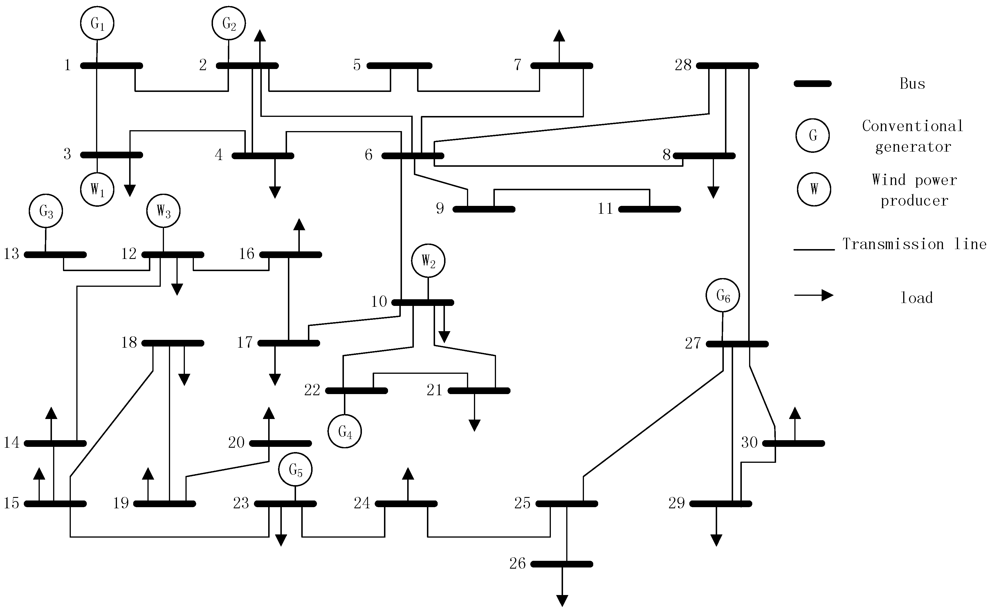
Besides, there is a contradiction between the minimization of system operating costs and the minimization of wind power curtailment, which cannot be achieved at the same time. In order to accommodate the deviation due to the uncertainty of wind power producers output, it is necessary to dispatch the output of conventional generators, which will increase the total operating cost of the system. If the wind power output deviation is not accommodated, it may result in excessive wind power curtailment. In order to make full use of renewable energy and analyze the relationship between two variables, the variable of curtailed wind power is introduced into the objective function to establish the bi-objective function of minimizing the system operation cost and the least wind power curtailment. Thus, the priority dispatching of renewable energy such as wind power can be ensured, reducing waste of resources. However, as suggested by the empirical findings, it should be noted that excessive attention to reducing wind power curtailment will increase system operating costs, revealing that it is necessary to weigh the importance of the two objective functions according to the actual situation. Finally, the low computing time (simulation on the IEEE 30-bus test system, with only 50.69 s to get the final result) makes the proposed method easy to promote, providing a reasonable test bed for the more realistic and complex electric market system.

References

1. Zhu, J. Optimization of Power System Operation; Wiley: Hoboken, NJ, USA, 2013. [Google Scholar]
2. Jin, X.; Chen, H. Model and Strategy of Source-Load Coordinated Dispatch Considering Intermittent Renewable Energy. South. Power Syst. Technol. 2015, 9, 2–6. [Google Scholar]
3. Liang, J.; Grijalva, S.; Harley, R.G. Increased Wind Revenue and System Security by Trading Wind Power in Energy and Regulation Reserve Markets. IEEE Trans. Sustain. Energy 2011, 2, 340–347. [Google Scholar] [CrossRef]
4. Meng, X.; Wang, H. Electric system scheduling in the condition of synchronization of large-scale wind power. J. Northeast. Electr. Univ. Nat. Sci. Ed. 2009, 29, 1–7. [Google Scholar]
5. Lei, Y. Studies on wind farm integration into power system. Autom. Electr. Power Syst. 2003, 27, 84–89. [Google Scholar]
6. Dai, H.; Wang, W.; Chi, Y. Recent wind power integration study in China. Power Syst. Technol. 2007, 31, 16–23. [Google Scholar]
7. Wu, C. Research on the influence of wind power on power balancing and reserve capacity. East China Electr. Power 2011, 39, 993–996. [Google Scholar]
8. Zhang, G.; Wu, W.; Zhang, B. Optimization of operational reserve coordination considering wind power integration. Autom. Electr. Power Syst. 2011, 35, 15–19. [Google Scholar]
9. Bobo, D.R.; Mauzy, D.M.; Trefny, F.J. Economic generation dispatch with responsive spinning reserve constraints. IEEE Trans. Power Syst. 1994, 9, 555–559. [Google Scholar] [CrossRef]
10. Fernandez-Blanco, R.; Arroyo, J.M.; Alguacil-Conde, N. On the Solution of Revenue- and Network-Constrained Day-Ahead Market Clearing under Marginal Pricing—Part II: Case Studies. IEEE Trans. Power Syst. 2017, 32, 220–227. [Google Scholar] [CrossRef]
11. Ceyhan, G.; Kurt, N.E.; Sahin, H.B.; Kürşad, D. Empirical comparison of three models for determining market clearing prices in Turkish day-ahead electricity market. In Proceedings of the European Energy Market, Dresden, Germany, 6–9 June 2017; IEEE: Piscataway, NJ, USA, 2017; pp. 1–7. [Google Scholar] [Green Version]
12. Abbaspourtorbati, F.; Conejo, A.; Wang, J.; Rachid, C. Pricing Electricity through a Stochastic Non-Convex Market-Clearing Model. IEEE Trans. Power Syst. 2017, 32, 1248–1259. [Google Scholar]
13. Shahidehpour, M.; Yamin, H.; Li, Z. Market Operations in Electric Power Systems: Forecasting, Dispatch, and Risk Management; IEEE Xplore: Austin, TX, USA, 2002. [Google Scholar]
14. Zheng, T.; Litvinov, E. Contingency-Based Zonal Reserve Modeling and Pricing in a Co-Optimized Energy and Reserve Market. IEEE Trans. Power Syst. 2008, 23, 277–286. [Google Scholar] [CrossRef]
15. Jiang, Y.; Chen, C. Particle Swarm Research of Stochastic Simulation for Unit Commitment in Wind Farms Integrated Power System. Trans. China Electrotech. Soc. 2009, 24, 129–137. [Google Scholar]
16. Zhou, W.; Peng, Y.; Sun, H. Optimal wind–thermal coordination dispatch based on risk reserve constraints. Eur. Trans. Electr. Power 2011, 21, 740–756. [Google Scholar] [CrossRef]
17. Fabbri, A.; Roman, T.G.S.; Abbad, J.R.; Quezada, V.H.M. Assessment of the cost associated with wind generation prediction errors in a liberalized electricity market. IEEE Trans. Power Syst. 2005, 20, 1440–1446. [Google Scholar] [CrossRef]
18. Yao, C.; Dong, Z.Y.; Meng, K.; Xu, Z.; Lu, H.H.-C.; Wong, K.P. Quantum-Inspired Particle Swarm Optimization for Power System Operations Considering Wind Power Uncertainty and Carbon Tax in Australia. IEEE Trans. Ind. Inform. 2012, 8, 880–888. [Google Scholar] [CrossRef]
19. Rockafellar, R.T.; Uryasev, S. Conditional value-at-risk for general loss distributions. J. Bank. Finan. 2002, 26, 1443–1471. [Google Scholar] [CrossRef] [Green Version]
20. Weng, Z.; Shi, L. Power System Dynamic Economic Dispatch Incorporating Wind Power Cost. Proc. CSEE 2014, 34, 514–523. [Google Scholar]
21. Hetzer, J.; Yu, D.C.; Bhattarai, K. An Economic Dispatch Model Incorporating Wind Power. IEEE Trans. Energy Convers. 2008, 23, 603–611. [Google Scholar] [CrossRef]
22. Morales, J.M.; Conejo, A.J.; Liu, K.; Zhong, J. Pricing Electricity in Pools with Wind Producers. IEEE Trans. Power Syst. 2012, 27, 1366–1376. [Google Scholar] [CrossRef] [Green Version]
23. Howard, R.A. Dynamic Programming. Manag. Sci. 1966, 12, 317–348. [Google Scholar] [CrossRef]
24. Ben-Tal, A.; Ghaoui, L.E.; Nemirovski, A. Robust Optimization; Princeton University Press: Princeton, NJ, USA, 2009. [Google Scholar]
25. Bertsimas, D.; Sim, M. The Price of Robustness. Oper. Res. 2004, 52, 35–53. [Google Scholar] [CrossRef]
26. Lorca, A.; Sun, X.A. Adaptive Robust Optimization with Dynamic Uncertainty Sets for Multi-Period Economic Dispatch under Significant Wind. IEEE Trans. Power Syst. 2015, 30, 1702–1713. [Google Scholar] [CrossRef]
27. Xie, L.; Gu, Y.; Zhu, X.; Genton, M.G. Short-Term Spatio-Temporal Wind Power Forecast in Robust Look-ahead Power System Dispatch. IEEE Trans. Smart Grid 2014, 5, 511–520. [Google Scholar] [CrossRef]
28. Li, Z.; Wu, W.; Zhang, B. A Robust Interval Economic Dispatch Method Accommodating Large-scale Wind Power Generation Part One—Dispatch Scheme and Mathematical Model. Autom. Electr. Power Syst. 2014, 38, 33–39. [Google Scholar]
29. Li, Z.; Wu, W.; Zhang, B. A Robust Interval Economic Dispatch Method Accommodating Large-scale Wind Power Generation Part Two—Uncertainty Set Modeling and Conservativeness Adjustment. Autom. Electr. Power Syst. 2014, 21, 32–38. [Google Scholar]
30. Ji, F.; Cai, X.; Yue, C. Fuzzy Robust Dispatch for Power Systems with Wind Farms. Proc. CSEE 2014, 34, 4791–4798. [Google Scholar]
31. Chen, J.; Wu, W. A Robust Interval Wind Power Dispatch Method Considering the Tradeoff between Security and Economy. Proc. CSEE 2014, 34, 1033–1040. [Google Scholar]
32. Zhao, H.; Wang, Y.; Zhao, M.; Tan, Q.; Guo, S. Day-Ahead Market Modeling for Strategic Wind Power Producers under Robust Market Clearing. Energies 2017, 10, 924. [Google Scholar] [CrossRef]
33. Zhao, H.; Wang, Y. Optimization Model of Residential Time-of-Use Tariff Calculation under Multi-Step Electricity Price. Electr. Power Constr. 2016, 37, 17–23. [Google Scholar]
34. Ye, H.; Wang, J.; Li, Z. MIP Reformulation for Max-min Problems in Two-stage Robust SCUC. IEEE Trans. Power Syst. 2016. [Google Scholar] [CrossRef]
35. Lei, M.; Zhang, J.; Dong, X.; Ye, J.J. Modeling the bids of wind power producers in the day-ahead market with stochastic market clearing. Sustain. Energy Technol. Assess. 2016, 16, 151–161. [Google Scholar] [CrossRef]
36. Abbaspourtorbati, F.; Conejo, A.J.; Wang, J.; Cherkaoui, R. Three- or Two-stage Stochastic Market-Clearing Algorithm? IEEE Trans. Power Syst. 2017, 32, 3099–3110. [Google Scholar] [CrossRef]
37. Wang, Q.; Wang, J.; Guan, Y. Price-Based Unit Commitment WITH Wind Power Utilization Constraints IEEE Trans. Power Syst. 2013, 28, 2718–2726. [Google Scholar] [CrossRef]
38. Aghaei, J.; Amjady, N.; Shayanfar, H.A. Multi-objective electricity market clearing considering dynamic security by lexicographic optimization and augmented epsilon constraint method. Appl. Soft Comput. 2011, 11, 3846–3858. [Google Scholar] [CrossRef]
39. Alonso, J.; Trias, A.; Gaitan, V.; Alba, J.J. Thermal plant bids and market clearing in an electricity pool minimization of costs vs. minimization of consumer payments. IEEE Trans. Power Syst. 1999, 14, 1327–1334. [Google Scholar] [CrossRef]
Figure 1. Diagram of IEEE 30-bus system.
Energies 11 01772 g001
Figure 2. The relationship between AVLMP and curtailed wind power.
Energies 11 01772 g002
Figure 3. Average clearing price of day-ahead market.
Energies 11 01772 g003