Article

Scaling Rules at Constant Frequency for Resonant Inductive Power Transfer Systems for Electric Vehicles

Department of Energy “G. Ferraris”, Politecnico di Torino, Corso Duca degli Abruzzi, 24, 10129 Torino, Italy
*
Author to whom correspondence should be addressed.
Energies 2018, 11(7), 1754; https://doi.org/10.3390/en11071754
Submission received: 6 June 2018 / Revised: 28 June 2018 / Accepted: 29 June 2018 / Published: 4 July 2018
(This article belongs to the Section F: Electrical Engineering)

Abstract

:
The paper proposes the development of a set of rules for the resizing of inductive power transfer systems with particular attention to the ones dedicated to the charge of electric vehicles. These rules aim at the construction of down-scaled prototypes allowing the study and the design with benefits in terms of costs, time consumption and flexibility. The theoretical results are experimentally validated by comparing a 1.1 kW system with its down-scaled version.

1. Introduction

The transmission of electrical energy through inductively coupled circuits, simply called inductive power transfer (IPT), is a hot research topic concerning several areas of technology. IPT is widespread among all applications where physical electrical connections cannot be used or when power is supplied to moving objects. IPT is then an effective solution for supplying power to body implanted medical devices [1,2], moving trolleys through defined paths [3,4] or underwater applications [5,6]. Currently, this technology is widely used for recharging mobile devices such as smartphones [7,8] or other daily used electronic devices [9,10]. This technology is easy to use and increases electrical safety and reliability thanks to the absence of electrical contacts. In the last few years, many research efforts have aimed at applying IPT to the charge of electric vehicles (EVs). In the near future, IPT systems for automotive applications may replace the standard plug-in chargers. These kinds of applications are commonly indicated as static IPT as they aim to charge the EV battery when the vehicle is stationary [11]. In the long run, the extension of the inductive charge during the movement of the vehicle, namely dynamic IPT, could represent an effective way to solve the current issues related to the battery i.e., limited range and the need for frequent and long stops for recharging [11].
IPT systems are mainly based on the same physical principles that govern the standard transformers. In the case of IPT systems for EVs, the primary coil is fixed at ground level and is usually called the transmitter. The secondary coil, called the receiver, is mounted under the vehicle floor so it is movable with respect to the transmitter. Unlike the standard transformer, the coupling takes place through a large air-gap on the order of some tens of centimeters. Hence, the flux is not constrained to a well defined path and the coupling between the two sides is typically lower than 30 % [12,13,14]. Ferrite bars are added to the coils in order to compensate for this coupling reduction. Conductive sheets, typically made of aluminum or steel, are used to guarantee the electromagnetic compatibility towards on-board electronic devices and to protect people in close proximity to the vehicle from electromagnetic field exposure. The typical power level of IPT systems goes from a few kilowatts, for household appliances, tens of kilowatts for the light EV charge, to hundreds of kilowatts for heavy EV charge. The frequency typically ranges from 10 kHz to 100 kHz .
The implementation of automotive IPT systems requires multidisciplinary expertise, involving, among others, magnetic field theory, power electronics, and mechanical engineering. Moreover, the prototyping of these systems is a time-consuming process that presents huge costs in terms of materials and manufacturing. This is why several works in the literature are based on small-size prototypes that can be easily constructed and rearranged [15,16,17]. Nevertheless, the applicability to real-size systems has not yet widely discussed and the relationships between the down-scaled prototypes and possible large-scale systems have not been analyzed.
The present paper deals with these issues by proposing a set of rules for the scaling of the IPT systems as done in the past for transformers [18] and electric motors [19,20]. These rules provide a powerful investigation tool that allows the study of an IPT system starting from a prototype of reduced dimensions. In this way, time and costs for prototype constructions can be strongly reduced with a significant benefit in flexibility and reconfigurability of the system. Furthermore, the use of a down-scaled prototype enables the work to be carried out with laboratory equipment at reduced voltages and currents resulting in an improvement of safety during the testing.

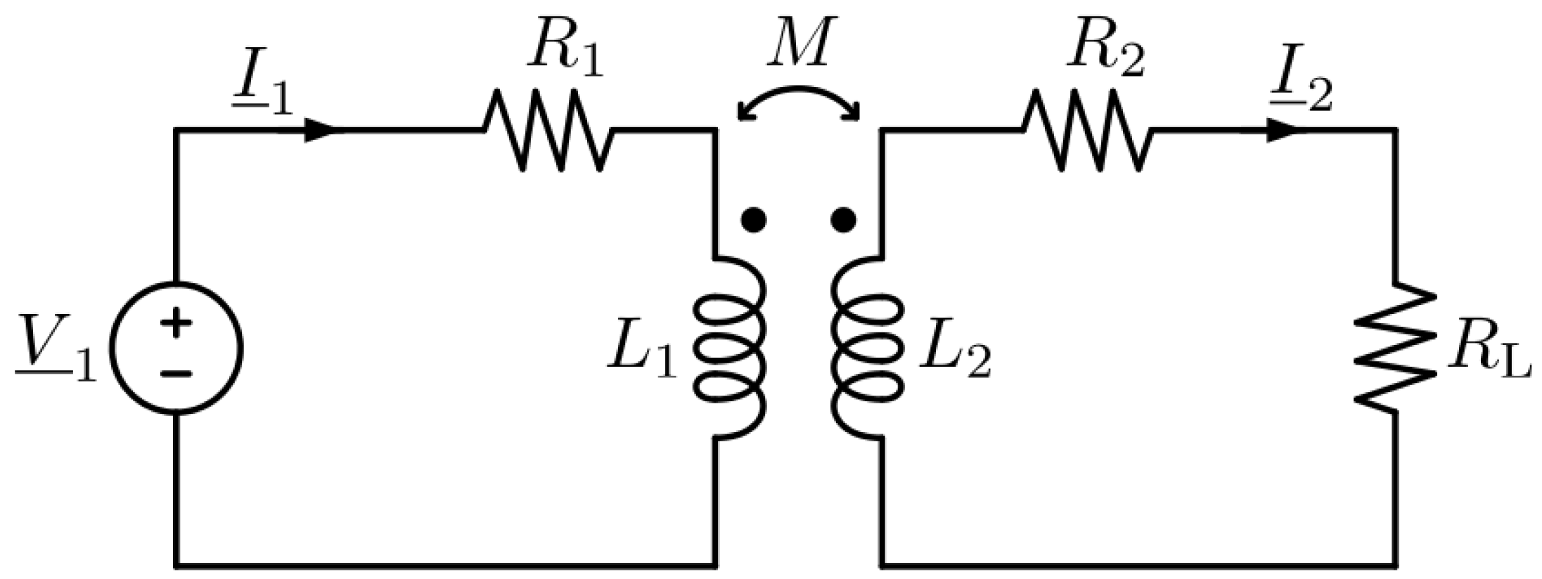
2. Circuit Model of Inductive Power Transfer System

The magnetic coupling between transmitter and receiver coils of an IPT system can be represented through the model shown in Figure 1. L 1 and L 2 represent the self-inductances of transmitter and receiver respectively and their magnetic coupling is modelled with the mutual inductance M. Resistors R 1 and R 2 represent the ohmic losses in the coils. By applying the fundamental harmonic approximation [21,22], the source is modelled with a sinusoidal voltage source of rms value V 1 and angular frequency ω . Since a rectifier and a filter are used at the receiver side [11,23,24], the load is represented through an equivalent resistance R L given by the ratio between the first harmonics of voltage and current at the rectifier terminals.
At the typical working frequencies of IPT systems, coil resistances can become relevant due to skin and proximity effect. This increase is compensated by constructing the coils using litz wire [25], a particular wire manufactured to guarantee a uniform distribution of the current density in the cross section. The use of litz wire together with a proper selection of the conductor section allows for considering R 1 and R 2 as negligible with respect to the magnitude of the impedances of the other components. This approximation, widely used in the domain of IPT [26,27,28], is here adopted in the following. The limits of validity of this assumption are discussed in Section 6.
Under the previous assumptions, the system of coupled inductors can be described by the following equations in the frequency domain:
{ (1) V ̲ 1 = j ω L 1 I ̲ 1 j ω M I ̲ 2 , (2) j ω M I ̲ 1 = j ω L 2 I ̲ 2 + R L I ̲ 2 .
The term on the left-hand side of Equation (2) represents the induced voltage in the receiver. This voltage can be measured at the receiver terminals under no-load conditions so it is called open-circuit voltage and indicated as V ̲ oc .
The ratio between the source voltage V ̲ 1 and current I ̲ 1 describes the equivalent impedance that the system shows at the source terminals. This impedance is called total impedance Z ^ T :
Z ^ T = V ̲ 1 I ̲ 1 = j ω L 1 + ω 2 M 2 j ω L 2 + R L .
The second term on the right-hand side of Equation (3) represents the effect that the coupled receiver has on the transmitter. This term is called the reflected impedance and it is defined as:
Z ^ R = ω 2 M 2 j ω L 2 + R L
It is worth noting that the denominator of the reflected impedance is equivalent to the impedance that the receiver shows to the dependent source V ̲ oc indicated as Z ^ 2 :
Z ^ 2 = j ω L 2 + R L .
The impedances Z ^ 2 and Z ^ T describe the relationships between currents and voltages at both sides of the system. Finally, the apparent power S 1 provided by the source and the apparent power S 2 transferred to the receiver are:
S 1 = V 1 I 1 = Z T I 1 2 ,
S 2 = V oc I 2 = ω 2 M 2 R L 2 + ( ω L 2 ) 2 I 1 2 = Z R I 1 2 .
It appears from the previous equations that the coils’ impedances represent a strong limitation in the power transfer capability as they limit the currents I 1 and I 2 . At the same time, the presence of these inductive impedances implies having a source with power rating S 1 higher than the transmissible real power P 1 . These reasons explain why, in IPT systems, the coil inductances are compensated through the connection of capacitive elements. The compensation capacitors can be connected in series or in parallel with the inductors or using different hybrid topologies [26,27]. The four basic compensation topologies are shown in Figure 2.
Independently of the compensation topology, the capacitors are chosen in order to obtain the cancellation of the inductive terms of Z ^ R and Z ^ T at a common angular frequency ω 0 that is the global resonance angular frequency of the IPT system. ω 0 is then the fundamental frequency of the source voltage V ̲ 1 .
For any basic compensation topology at the receiver side, the capacitor C 2 is chosen according to the relationship:
C 2 = 1 ω 0 2 L 2 .
Because the capacitor is placed in the circuit, at the resonance, the impedance Z ^ 2 becomes equal to R L and the reflected impedance can be expressed as:
Z ^ R = ω 0 2 M 2 R L for   series   compensated   receiver ,
Z ^ R = M 2 R L L 2 2 j ω 0 M 2 L 2 for   parallel   compensated   receiver .
The capacitor C 1 is chosen according to the relationships indicated in Table 1 in order to compensate the self-inductance of the transmitter plus the imaginary component of Z ^ R . In these conditions, the value of Z ^ T equals the real component of Z ^ R . As the total impedance at the resonance is real, the source has only the real power P 1 then:
S 1 = P 1 = Z R I 1 2 .
Having neglected the losses, P 1 equals the power P 2 transferred to the load.

3. Derivation of Scaling Rules

Let d be a generic linear dimension of the starting structure and d the corresponding dimension of the scaled one. The scaling factor γ is defined as:
γ = d d .
A value γ < 1 corresponds to a down scaling of the original structure. This scaling factor is applied to all the geometric dimensions of the IPT structure. A scaling process can be conducted by considering different constraints for the electrical parameters. In the present work, the scaling of the electrical parameters is derived according to the following hypotheses:
  • The working frequency ω 0 and the current density remain constant in the scaling process. This assumption allows for considering the same exploitation of the conductors material. Moreover, keeping the frequency fixed allows for operating with similar characteristics of the power electronics drivers and control.
  • The number of turns of transmitter and receiver coils does not change in the scaling process. This assumption guarantees that the re-sized structure changes only in the dimensions while the constructive characteristics are left unchanged.

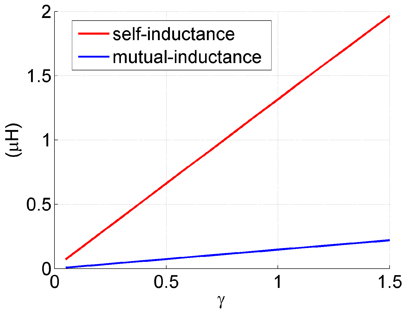
3.1. Scaling of Self and Mutual Inductance

The derivation of the scaling rules for the inductive parameters requires some additional insight. A generic inductance in free space can be calculated starting from the Neumann’s formula for filamentary coils [29]:
L j k = μ 0 4 π N j N k Γ j Γ k u j · u k | r j k | d l j d l k ,
where the integrals are extended to the wire paths Γ j and Γ k . d l j and d l k represent the elementary coil lengths along the integration paths whose distance is | r j k | . Equation (13) provides the self-inductance when j = k ; otherwise, it expresses the mutual inductance between two different coils. According to Equation (13), d l j , d l k and | r j k | being linear dimensions, the relationship
L j k γ
holds true.
While Equation (13) applies to inductors in free space, the coils of an IPT system for EV applications are usually embedded in complex environments where conductive and ferromagnetic materials are present. The magnetic field distribution is influenced by the presence of the vehicle chassis that usually exhibits a predominant conductive behaviour [30,31]. Moreover, aluminium shields are often used to confine the magnetic field for electromagnetic compatibility reasons while magnetic materials can be used to guide the magnetic flux, increasing the coupling and improving the tolerance to transmitter–receiver misalignments [13,14,32].
By following a similar approach to the one proposed in [23,32], the magnetic structure of the IPT system can be described through a series of flux tubes that define a network of reluctances. Hence, self and mutual inductances can be considered inversely proportional to the reluctance R of the overall magnetic flux path:
R = l μ S ,
where l is the length of the flux path, S is its cross section and μ is the equivalent magnetic permeability. Although the presence of a large air-gap makes the definition of l and S difficult, the following relationship can be considered true in first approximation:
L j k = N j N k R = N j N k μ S l γ .
The validity of Equation (16) is detailed in Appendix A.

3.2. Scaling of Currents, Voltages and Power

Under the assumption of constant current density in the coils during the scaling process, the generic current I i can be expressed as:
I i = J i S wire , i γ 2 ,
J i being the current density in the generic coil and S wire , i the cross section of the wire.
According to Equations (16) and (17), the open-circuit voltage is
V oc = ω 0 M I 1 γ 3 .
Hence, the apparent power delivered to the receiver defined in Equation (7) follows the rule:
S 2 V oc I 2 γ 5 .
At the resonance, the apparent power S 2 equals the active power P 2 . Since the transmitted power is proportional to the source power S 1 (or, equivalently, P 1 ), this power follows the same proportionality with respect to γ . Hence, according to Equation (6), the source voltage has to be scaled as:
V 1 γ 3 .
Having put in evidence that voltages and currents are dependent on different powers of γ , the equivalent load has to be modified according to the relationship:
R L γ .
This relationship can be verified also by looking at Equations (9) and (10). These relationships indicate that total and reflected impedance follow the same proportionality rule of R L .

3.3. Scaling of the Compensation Capacitances

The results carried out for the load and the reflected impedance confirmed that, having considered the working frequency fixed, the value of the compensation capacitors depends only on the value of the magnetic parameters of the coils (i.e., self and mutual inductances). Hence, the relationship
C i 1 γ
is valid for both the compensation capacitors on the transmitter and receiver side. Furthermore, this rule has a general validity as can be verified by considering the relationships for the different compensation topologies reported in Table 1.
The electrical stress over the capacitors is one of the key points that justifies the use of down-scaled prototypes. The typical values of tens of kilohertz for the frequency and the tens of nanofarad used for the compensation capacitors [23,32,33] lead to voltages across the capacitors that can reach several kilovolts. According to Equations (17) and (22), the voltages over the capacitors also scale as γ 3 . This strong reduction introduces an important benefit in terms of safety against possible electric hazards or insulation failures during the tests. At the same time, the reduced necessities in terms of current and voltage allow the adoption of cheap and easily available capacitors.

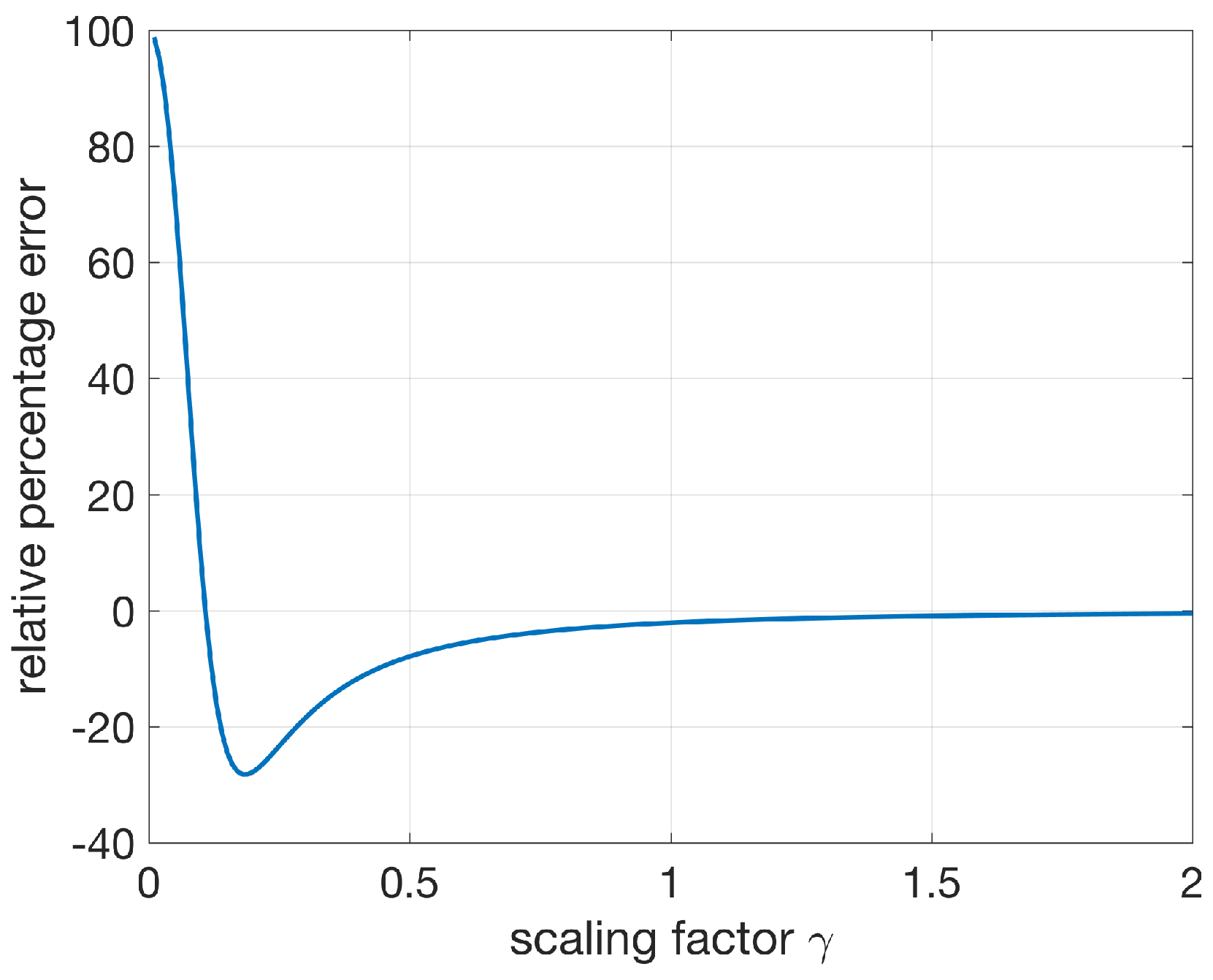
4. Scaling-Rules’ Limits of Validity

4.1. Coil Resistances

The set of rules for the IPT systems scaling has been developed neglecting the system losses. Clearly, this assumption is not respected when γ 1 i.e., for a significative down scaling. Assuming a constant and uniform current density distribution in the conductors, the resizing relationship for the coils resistances reads:
R i = ρ i l i S wire , i 1 γ .
Hence, there is a certain limit in the down scaling beyond which the amplitude of the coils resistances is no more negligible with respect to the impedances of the other parameters of the system. This limit value of γ < 1 depends on the characteristics of the original system, and then it has to be evaluated on a case by case basis.

4.2. Capacitors’ ESR

In a resizing process, the capacitor losses deserve particular consideration as well as the coil resistances. The capacitors’ losses are accounted for with the equivalent series resistance (ESR). In the resizing process, the modification of the capacitance value, together with the change of applied voltages and currents, make the change of the capacitor technology necessary. In this case, the value of the ESR can not be put in relation to the geometrical parameters of the components as it depends also on the manufacturing technology and the characteristics of the dielectric material [34]. According to these considerations, it is practically impossible to find a generic rule for the resizing of the capacitor resistive component. The incidence of these parameters needs to be individually considered. However, it is worth nothing that, contrary to what happens for the coil resistances, the ESR tends to become less relevant for capacitors of small dimension.

5. Power Losses and Efficiency

The variation of the efficiency with the change of the IPT system dimensions can be separately investigated by considering the main components responsible for losses. These losses can be separated into losses in conductive materials and losses in ferromagnetic materials. They are indicated as P J and P Fe , respectively. According to the hypothesis of constant current density, it is possible to assume that the conductive losses are proportional to the volume of the conductive material:
P J = R i I i 2 = ρ i l i S wire , i J i S wire , i 2 = ρ i l i S wire , i J i 2 γ 3 .
The definition of ferromagnetic losses requires some additional insight as their formulation is not unique and depends on several parameters related to material properties and characteristics of the exciting sources. According to the typical sinusoidal waveform of the currents in IPT systems, the Steinmetz formulation [35], commonly used in the design of electrical machines [36,37,38,39], is here adopted:
P Fe = V Fe K f α B ^ β .
This formulation states that the losses into a ferromagnetic material, under sinusoidal excitation, are dependent on the volume of material V Fe and power functions of the sinusoidal excitation frequency f and the peak of the magnetic flux density B ^ . K, α and β are positive numbers whose values depend on the material. In an homogeneous medium, the magnetic flux density is proportional to the source current and inversely proportional to the distance from the source, hence:
B γ .
In Appendix A, it is shown that this relationship is still valid when linear ferromagnetic objects are located in proximity of the source.
The volume of material depends on the third power of γ , thus it is possible to express the ferromagnetic losses as:
P Fe γ 3 · γ β = γ 3 + β .
Gathering all the γ -independent parameters of losses in three constants c 1 , c 2 and c 3 , it is possible to provide a general expression for the efficiency:
η = P 2 P 2 + P J + P Fe c 1 γ 5 c 1 γ 5 + c 2 γ 3 + c 3 γ 3 + β .
Differently from all previous scaling relationships, in Equation (28), it is not possible to directly correlate the efficiency with a precise power function of γ . This relationship can directly provide information on the asymptotic behaviour (i.e., for γ + and γ 0 ) while the efficiency of the scaled system can be estimated only after the evaluation of each term of Equation (28).

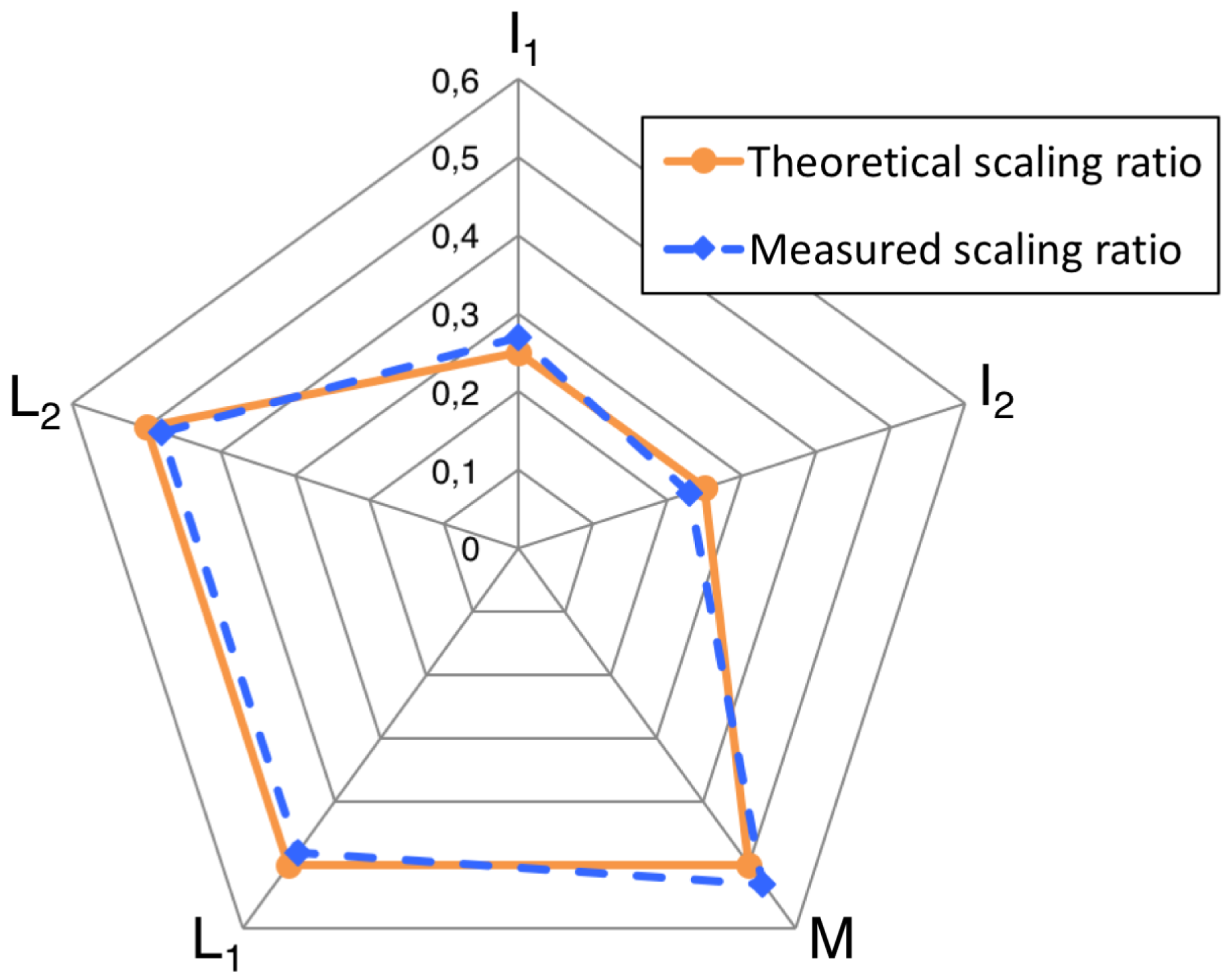
6. Experimental Validation

The scaling rules are experimentally validated by constructing a starting IPT system and its down-scaled version. The starting system consists of two identical rectangular coils made by arranging the litz wire windings in two overlapping layers. A core made of several I-shape 3F3 ferrite bars is put on the receiver side only. The geometrical characteristics are reported in Table 2. The second IPT system is built by applying a scaling factor γ = 0.5 to the original system. The two systems are shown in Figure 3.
In both configurations, the transmitter is supplied by a mosfet based H-bridge providing a square wave voltage at a fixed frequency of 110 kHz . This frequency is then the resonance frequency for both systems.
The self inductance of each coil and the related resistances at the resonance frequency are measured by using the HIOKI 3532-50 LCR HiTESTER impedance meter (HIoki E.E. Corporation, Nagano, Japan). The mutual inductance between transmitter and receiver coils is measured by supplying the system with a sinusoidal signal amplified through a linear amplifier in no load conditions. The current in the transmitter and the open-circuit voltage at the receiver terminals are measured through a LeCroy Wavesurfer 3024 8 bit digital oscilloscope (Teledyne LeCroy, Chestnut Ridge, NY, USA). Hence, the value of mutual inductance is calculated by applying Equation (2). The results of the measurements are used to evaluate the experimental scaling factor obtained with the down-scaled prototype. The results are reported in Table 3 where the ratio between the quantities of the original system and the respective quantities of the scaled one are referred to as scaling ratio. The values of the self inductances have been used to choose the proper compensation capacitors, on the bases of Equation (8) and Table 1, by applying a series–series compensation. The exact value of capacitance has been obtained by a series and parallel connection of several capacitors of the same technology.
Starting from the measured parameters, it is possible to investigate the limits of the scaling rules for the starting system verifying also that the down-scaled system reasonably remains within these limits. Taking into account the coil resistances, it is possible to rewrite the total impedance of the series-series compensated system as:
Z ^ T = R 1 + j ω L 1 1 ω C 1 + ω 2 M 2 j ω L 2 1 ω C 1 + R 2 + R L .
At the resonance, this expression simplifies as:
Z T = R 1 + ω 0 2 M 2 R 2 + R L .
The difference between the lossless and lossy behaviour of the total impedance is shown in Figure 4. It is visible that the lossy behaviour is assimilable to the lossless one as long as the value of the coil resistances remain lower than the load resistance. The relative error introduced by the lossless approximation for different values of the scaling factor is shown in Figure 5. This graph indicates that the gap between the lossless and the lossy behaviour of Z T becomes relevant for scaling factors lower than about 0.3. For lower values of γ , the effect of the losses becomes predominant and the scaling rules start to overcome the limits of validity. In the adopted down-scaled system for the experimental verification, the application of a scaling factor γ = 0.5 corresponds to a relative error of about 8 % on the value of the total impedance.
Finally, the two IPT systems have been fully powered through the H-bridge whose DC bus voltage has been regulated according to Equation (20). The values of the DC bus voltage and coil currents are reported in Table 4. The effects of the down-scaling on the main system parameters are graphically summarised in Figure 6. This graph shows a good agreement of the results with respect to the expected values. A maximum error of 8 % is found in the evaluation of the currents. The error on the mutual and self-inductances is of 6 % and 4 % , respectively.

6.1. Power and Losses

The source power P 1 and the power P 2 transferred to the load are evaluated on the basis of measured waveforms at the H-bridge output and over the system load. Then, the overall losses P loss are evaluated as the difference between P 1 and P 2 . Having the measurement of the current in each coil, it is possible to evaluate the conductive losses P J on each side of the system. The remaining losses are attributed to the ferrite obtaining an estimation of P Fe . As the adopted ferrite presents a parameter β = 2.71 , it is possible to expect a scaling of the losses in the ferromagnetic material as:
P Fe γ 3 + 2.71 = γ 5.71 .
The obtained results are collected in Table 5. The results confirm that the developed relations can provide reliable predictions on the losses for a scaling process. The obtained errors on the expected scaling ratios are of 19.2 % and 17.7 % on conductive and ferromagnetic losses, respectively. These power measurements are more sensitive to measurement errors than the measurements on voltages and currents, but the obtained results can be still considered valid from an engineering point of view.
Finally, thanks to the measurements of transmitted power and losses, it is possible to evaluate the efficiency of the two systems. The results are shown in Table 6. Moreover, it is possible to use the relations provided in Section 5 in order to verify the possibility of an estimation of the scaled system efficiency by using the relation:
η scaled = γ 5 P 2 origin γ 5 P 2 origin + γ 3 P J origin + γ 5.71 P Fe origin
From Equation (32), an efficiency of the down-scaled system of 0.794 is obtained. This value has an error of 0.63 % with respect to the measured efficiency of the scaled system.
It is worth noting that the values of power losses and efficiency of the down-scaled system are effected by large measurement errors. In high efficiency systems, such as IPT ones, power losses are usually low and, in the down-scaled system, can assume values that are comparable with the power meter resolution.

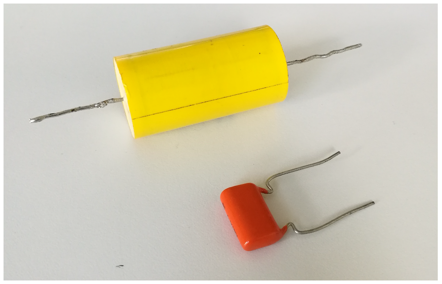
6.2. Compensation Capacitors’ Technology

As already pointed out in Section 4.2, the down-scaling process causes an increase of the compensation capacitors values by a factor γ 1 while the voltage drop across these components decreases with a factor γ 3 . For the systems under study, the voltage across the capacitor on the receiver side is reduced from 1.285 kV to 138 V . The compensation of the original system has been done by using several high-voltage high-current film capacitors as typically done in IPT for EV applications [24,40] while more common and less expensive ceramic capacitors have been used for the down-scaled system. Two samples of the adopted capacitors are shown in Figure 7. The ESR of both capacitors has been measured by using the same impedance meter used for the measurements over the coils. The results of Table 7 point out that the ESR is not correlated with the scaling factor. At the same time, the measurements confirm that the losses of the capacitors are negligible with respect to the losses in the coils.

7. Conclusions

The paper has presented a set of rules for the scaling of high power IPT systems. This set of rules has been proven, by experimental and numerical validation, to be a simple and effective tool that is well suited to the study of IPT systems for EVs. In their range of validity, these rules can predict, with reliable precision, the steady-state behavior of a full scale system using a down-scaled prototype. The same rules could also be useful for the design of new IPT systems starting from an existent one as is usually done for standard electric machines. The developed rules were experimentally verified by comparing an original IPT system having a rated power of 1.1 kW with its down-scaled version whose linear dimensions were half of the original system. The experimental assessment indicated that the application of the scaling rules introduces admissible errors when the down-scaled dimensions remain below 50 % of the original linear dimensions.
The study confirms the validity and the benefits of the presented rules for the construction of down-scaled prototypes. The most relevant benefit is represented by the increase of electrical safety of the testing setup. In fact, the high voltage drop over the compensation capacitors has been reduced by an order of magnitude. In addition, the power rating of the source has also been strongly reduced. In the analyzed case, we were able to predict the behavior of a system with a source power rating in the order of kilowatts by using a power supply of a few tens of watts.
Finally, the cost of the prototype has been reduced to approximately one-tenth of the cost of the original system due to the reduced quantity of materials. This cost reduction is also accompanied by a strong increase of the flexibility and reconfigurability of the system.

Author Contributions

All the authors gave their contribution to all of the aspects of the manuscript.

Funding

This research received no external funding.

Conflicts of Interest

The authors declare no conflict of interest.

Appendix A. Scaling of Inductances in Complex Environment

A numerical example case is studied to investigate the assumptions proposed in the paper relating the scaling of magnetic parameters. The results are based on an axisymmetric IPT system simulated using the finite elements method software FEMM (version 4.2) [41].The IPT system is shown in Figure A1. It is composed by two coils with different radii and a ferrite plate placed above an aluminium plate. The original dimensions of the system and the materials properties are reported in Table A1. The starting IPT system is then simulated by applying different scaling factors. Only the transmitter is energised by supplying the current I tr . For each value of γ , the self-inductance is evaluated as:
L = 1 I tr 2 Ω tr A · J d Ω ,
where Ω tr is the cross-section of the transmitter coil and A and J are the magnetic vector potential and the current density over the conductor cross section. The mutual inductance is evaluated by integrating the magnetic vector potential due to the current flowing in the transmitter over the receiver coil cross section Ω re :
M = 1 I tr Ω re Ω re A · d Ω .
The results shown in Figure A2 confirm the validity of Equation (16) i.e., the self and mutual inductances vary linearly with γ also with complex environments. The same numerical example allows for investigating the behaviour of the magnetic flux density into the ferrite. Figure A3 shows the variation of the average value of magnetic flux density in the ferrite plate during the scaling process. The results confirm the validity of the relation of proportionality described through Equation (26) for a not saturated material.
Figure A3 also states that saturation of the magnetic material does not affect the down-scaled systems, where the magnetic flux density decreases with respect to the original system. However, the saturation does not represent a real limitation in IPT systems for EVs even in case of up-scaling. In these kinds of systems, the ferrite is inserted in order to shape the magnetic field in order to maximize the coupling between the transmitter and the receiver. This is possible if the ferrite offers a low-reluctance path while the majority of the magnetic flux path consists of air. Because of this, the section of the ferrite core has to be typically oversized in order to have an appreciable impact on the magnetic circuit. This, in turn, determines a low magnetic flux density inside the ferrite, which is far from the saturation levels and would work in the linear part of the magnetic characteristic also if the original dimensions of the system are doubled.
Figure A1. 3D view of the axisymmetric model for magnetic simulation.
Energies 11 01754 g0a1
Figure A2. Mutual inductance and transmitter self-inductance versus the scaling factor.
Energies 11 01754 g0a2
Figure A3. Mean magnetic flux density in the ferrite versus the scaling factor.
Energies 11 01754 g0a3
For the sake of completeness, an approach aimed to keep the magnetic flux density constant during the scaling is proposed here. It consists of increasing the only thickness of the ferrite following the proportionality to γ 2 (and not simply γ as well as the others linear dimensions). This forces the ferrite section to scale as γ 3 . However, according to the same considerations made before, this will have a negligible impact on the scaling of self and mutual inductances. This assumption has been proved by means of the same numerical case of Figure A1. As visible in Figure A4 and Figure A5, with the proposed approach, the inductances still scale linearly while the induction remains practically constant.
Table A1. Simulated IPT system parameters.
ParameterValue
Transmitter radius 400 mm
Transmitter wire diameter 10 mm
Receiver radius 350 mm
Receiver wire diameter 10 mm
Coils distance 200 mm
Ferrite plate inner rad. 100 mm
Ferrite plate outer rad. 450 mm
Ferrite plate thickness 20 mm
Aluminium plate radius 500 mm
Aluminium plate thickness 1 mm
Aluminium-Ferrite plates dist. 10 mm
Ferrite magnetic permeability2000
Ferrite conductivity 0.2 S / m
Aluminium conductivity 34 MS / m
Figure A4. Mutual inductance and transmitter self-inductance versus the scaling factor for ferrite thickness proportional to γ 2 .
Energies 11 01754 g0a4
Figure A5. Mean magnetic flux density in the ferrite versus the scaling factor for ferrite thickness proportional to γ 2 .
Energies 11 01754 g0a5
If both current density and magnetic flux density are kept constant, the losses in conductive and ferromagnetic materials depend only on the volume of material. Hence, the relationship for the scaling of the efficiency reads:
η = P 2 P 2 + P J + P Fe c 1 γ 5 c 1 γ 5 + c 2 γ 3 + c 3 γ 4 ,
where the term P J remains proportional to γ 3 while P Fe is forced to follow the proportionality with γ 4 . In this case, this relationship clearly indicates that the efficiency tends to always increase if the dimensions of the IPT system increase.

References

  1. Lu, Y.; Ma, D.B. Wireless power transfer system architectures for portable or implantable applications. Energies 2016, 9, 1087. [Google Scholar] [CrossRef]
  2. Park, S.; Kim, H.; Cho, J.; Kim, E.; Jung, S. Wireless power transmission characteristics for implantable devices inside a human body. In Proceedings of the 2014 International Symposium on Electromagnetic Compatibility (EMC Europe), Gothenburg, Sweden, 1–4 September 2014; pp. 1190–1194. [Google Scholar]
  3. Green, A.W.; Boys, J.T. An inductively coupled high frequency power system for material handling applications. In Proceedings of the IPEC Conference, Singapore, 18–19 March 1993; Volume 2, pp. 821–826. [Google Scholar]
  4. Tampubolon, M.; Pamungkas, L.; Chiu, H.J.; Liu, Y.C.; Hsieh, Y.C. Dynamic Wireless Power Transfer for Logistic Robots. Energies 2018, 11, 527. [Google Scholar] [CrossRef]
  5. Radecki, A.; Chung, H.; Yoshida, Y.; Miura, N.; Shidei, T.; Ishikuro, H.; Kuroda, T. 6 W/25 mm2 inductive power transfer for non-contact wafer-level testing. In Proceedings of the 2011 IEEE International Solid-State Circuits Conference, San Francisco, CA, USA, 20–24 February 2011; pp. 230–232. [Google Scholar]
  6. Cheng, Z.; Lei, Y.; Song, K.; Zhu, C. Design and loss analysis of loosely coupled transformer for an underwater high-power inductive power transfer system. IEEE Trans. Magn. 2015, 51, 1–10. [Google Scholar]
  7. Waffenschmidt, E. Wireless power for mobile devices. In Proceedings of the 2011 IEEE 33rd International Telecommunications Energy Conference (INTELEC), Amsterdam, The Netherlands, 9–13 October 2011; pp. 1–9. [Google Scholar]
  8. Uchida, A.; Shimokawa, S.; Kawano, H.; Ozaki, K.; Matsui, K.; Taguchi, M. Phase and intensity control of multiple coil currents in mid-range wireless power transfer. IET Microw. Antennas Propag. 2014, 8, 498–505. [Google Scholar] [CrossRef]
  9. Raval, P.; Kacprzak, D.; Hu, A.P. A wireless power transfer system for low power electronics charging applications. In Proceedings of the 2011 6th IEEE Conference on Industrial Electronics and Applications (ICIEA), Beijing, China, 21–23 June 2011; pp. 520–525. [Google Scholar]
  10. Jonah, O.; Georgakopoulos, S.V.; Tentzeris, M.M. Wireless power transfer to mobile wearable device via resonance magnetic. In Proceedings of the 2013 IEEE 14th Annual Wireless and Microwave Technology Conference (WAMICON), Orlando, FL, USA, 7–9 April 2013; pp. 1–3. [Google Scholar]
  11. Bi, Z.; Kan, T.; Mi, C.C.; Zhang, Y.; Zhao, Z.; Keoleian, G.A. A review of wireless power transfer for electric vehicles: Prospects to enhance sustainable mobility. Appl. Energy 2016, 179, 413–425. [Google Scholar] [CrossRef] [Green Version]
  12. Bosshard, R.; Iruretagoyena, U.; Kolar, J.W. Comprehensive Evaluation of Rectangular and Double-D Coil Geometry for 50 kW/85 kHz IPT System. IEEE J. Emerg. Sel. Top. Power Electron. 2016, 4, 406–1415. [Google Scholar] [CrossRef]
  13. Zhang, W.; White, J.C.; Abraham, A.M.; Mi, C.C. Loosely Coupled Transformer Structure and Interoperability Study for EV Wireless Charging Systems. IEEE Trans. Power Electron. 2011, 30, 6356–6367. [Google Scholar] [CrossRef]
  14. Budhia, M.; Covic, G.A.; Boys, J.T. Design and Optimization of Circular Magnetic Structures for Lumped Inductive Power Transfer Systems. IEEE Trans. Power Electron. 2011, 26, 3096–3108. [Google Scholar] [CrossRef]
  15. Liu, J.; Chan, K.W.; Chung, C.Y.; Chan, N.H.L.; Liu, M.; Xu, W. Single-Stage Wireless-Power-Transfer Resonant Converter with Boost Bridgeless Power-Factor-Correction Rectifier. IEEE Trans. Ind. Electron. 2018, 65, 2145–2155. [Google Scholar] [CrossRef]
  16. Geng, Y.; Li, B.; Yang, Z.; Lin, F.; Sun, H. A high efficiency charging strategy for a supercapacitor using a wireless power transfer system based on inductor/capacitor/capacitor (LCC) compensation topology. Energies 2017, 10, 135. [Google Scholar] [CrossRef]
  17. Li, M.; Chen, Q.; Hou, J.; Chen, W.; Ruan, X. 8-Type contactless transformer applied in railway inductive power transfer system. In Proceedings of the IEEE Energy Conversion Congress and Exposition, Denver, CO, USA, 15–19 September 2013; pp. 2233–2238. [Google Scholar]
  18. Zakrzewski, K.; Tomczuk, B.; Waindok, A. Nonlinear scaled models in 3D calculation of transformer magnetic circuits. Int. J. Comput. Math. Electr. Electron. Eng. 2006, 25, 91–101. [Google Scholar] [CrossRef]
  19. Stipetic, S.; Zarko, D.; Popescu, M. Scaling laws for synchronous permanent magnet machines. In Proceedings of the 2015 Tenth International Conference on Ecological Vehicles and Renewable Energies (EVER), Monte Carlo, Monaco, 31 March–2 April 2015; pp. 1–7. [Google Scholar]
  20. Reichert, T.; Nussbaumer, T.; Kolar, J.W. Torque scaling laws for interior and exterior rotor permanent magnet machines. In Proceedings of the IEEE International Magnetics Conference 2009 (INTERMAG 2009), Sacramento, CA, USA, 4–8 May 2009; p. 3. [Google Scholar]
  21. De Simone, S.; Adragna, C.; Spini, C.; Gattavari, G. Design-oriented steady-state analysis of LLC resonant converters based on FHA. In Proceedings of the International Symposium on Power Electronics, Electrical Drives, Automation and Motion (SPEEDAM 2006), Taormina, Italy, 23–26 May 2006; pp. 200–207. [Google Scholar]
  22. Hua, C.C.; Fang, Y.H.; Lin, C.W. LLC resonant converter for electric vehicle battery chargers. IET Power Electron. 2016, 9, 2369–2376. [Google Scholar] [CrossRef]
  23. Huh, J.; Lee, S.W.; Lee, W.Y.; Cho, G.H.; Rim, C.T. Narrow-width inductive power transfer system for online electrical vehicles. IEEE Trans. Power Electron. 2011, 26, 3666–3679. [Google Scholar] [CrossRef]
  24. Del Toro García, X.; Vázquez, J.; Roncero-Sánchez, P. Design implementation issues and performance of an inductive power transfer system for electric vehicle chargers with series-series compensation. IET Power Electron. 2015, 8, 1920–1930. [Google Scholar] [CrossRef]
  25. Wojda, R.P.; Kazimierczuk, M.K. Winding resistance of litz-wire and multi-strand inductors. IET Power Electron. 2012, 5, 257–268. [Google Scholar] [CrossRef]
  26. Li, S.; Li, W.; Deng, J.; Nguyen, T.D.; Mi, C.C. A double-sided LCC compensation network and its tuning method for wireless power transfer. IEEE Trans. Veh. Technol. 2015, 64, 2261–2273. [Google Scholar] [CrossRef]
  27. Villa, J.L.; Sallan, J.; Osorio, J.F.S.; Llombart, A. High-misalignment tolerant compensation topology for ICPT systems. IEEE Trans. Ind. Electron. 2012, 59, 945–951. [Google Scholar] [CrossRef]
  28. Wang, C.S.; Covic, G.A.; Stielau, O.H. Power transfer capability and bifurcation phenomena of loosely coupled inductive power transfer systems. IEEE Trans. Ind. Electron. 2004, 51, 148–157. [Google Scholar] [CrossRef]
  29. Paul, C.R. Inductance: Loop and Partial; John Wiley & Sons: Hoboken, NJ, USA, 2011; ISBN 9780470461884. [Google Scholar]
  30. Ibrahim, M.; Pichon, L.; Bernard, L.; Razek, A.; Houivet, J.; Cayol, O. Advanced modeling of a 2-kW series-series resonating inductive charger for real electric vehicle. IEEE Trans. Veh. Technol. 2015, 64, 421–430. [Google Scholar] [CrossRef]
  31. Bavastro, D.; Canova, A.; Cirimele, V.; Freschi, F.; Giaccone, L.; Guglielmi, P.; Repetto, M. Design of wireless power transmission for a charge while driving system. IEEE Trans. Magn. 2014, 50, 965–968. [Google Scholar] [CrossRef]
  32. Shin, J.; Shin, S.; Kim, Y.; Ahn, S.; Lee, S.; Jung, G.; Cho, D.H. Design and Implementation of Shaped Magnetic-Resonance-Based Wireless Power Transfer System for Roadway-Powered Moving Electric Vehicles. IEEE Trans. Ind. Electron. 2014, 61, 1179–1192. [Google Scholar] [CrossRef]
  33. Pevere, A.; Petrella, R.; Mi, C.C.; Zhou, S. Design of a high efficiency 22 kW wireless power transfer system for EVs fast contactless charging stations. In Proceedings of the 2014 IEEE International Electric Vehicle Conference (IEVC), Florence, Italy, 17–19 December 2014; pp. 1–7. [Google Scholar]
  34. Spyker, R.L.; Nelms, R.M. Classical equivalent circuit parameters for a double-layer capacitor. IEEE Trans. Aerosp. Electron. Syst. 2000, 36, 829–836. [Google Scholar] [CrossRef]
  35. Steinmetz, C.P. On the law of hysteresis. Trans. Am. Inst. Electr. Eng. 1892, 9, 1–64. [Google Scholar] [CrossRef]
  36. Reinert, J.; Brockmeyer, A.; De Doncker, R.W. Calculation of losses in ferro- and ferromagnetic materials based on the modified Steinmetz equation. IEEE Trans. Ind. Appl. 2001, 37, 1055–1061. [Google Scholar] [CrossRef]
  37. Venkatachalam, K.; Sullivan, C.R.; Abdallah, T.; Tacca, H. Accurate prediction of ferrite core loss with nonsinusoidal waveforms using only Steinmetz parameters. In Proceedings of the IEEE Workshop on Computers in Power Electronics, Mayaguez, PR, USA, 3–4 June 2002; pp. 36–41. [Google Scholar]
  38. Boglietti, A.; Cavagnino, A.; Lazzari, M.; Pastorelli, M. Predicting iron losses in soft magnetic materials with arbitrary voltage supply: An engineering approach. IEEE Trans. Magn. 2003, 39, 981–989. [Google Scholar] [CrossRef]
  39. Kim, Y.T.; Cho, G.W.; Kim, G.T. The estimation method comparison of iron loss coefficients through the iron loss calculation. J. Electr. Eng. Technol. 2013, 8, 1409–1414. [Google Scholar] [CrossRef]
  40. Sallan, J.; Villa, J.L.; Llombart, A.; Sanz, J.F. Optimal design of ICPT systems applied to electric vehicle battery charge. IEEE Trans. Ind. Electron. 2009, 56, 2140–2149. [Google Scholar] [CrossRef]
  41. Meeker, D.C. Finite Element Method Magnetics, Version 4.2. Available online: http://www.femm.info (accessed on 2 July 2018).
Figure 1. Circuit model of two coupled inductors with the sinusoidal voltage source of amplitude V 1 and the equivalent load R L .
Energies 11 01754 g001
Figure 2. Circuit representation of the four basic compensation topologies.
Energies 11 01754 g002
Figure 3. Tested inductive power transfer (IPT) systems. Starting system (a) and down-scaled one (b).
Energies 11 01754 g003
Figure 4. Coil resistances, equivalent load and total impedance of the starting system versus scaling factor.
Energies 11 01754 g004
Figure 5. Relative error of lossless total impedance with respect to the lossy one.
Energies 11 01754 g005
Figure 6. Comparison of theoretical and actual scaling ratios for self-inductances, mutual inductance and coils currents obtained downstream of the down-scaling.
Energies 11 01754 g006
Figure 7. Adopted compensation capacitors. High-voltage film capacitor in yellow. Ceramic capacitor in orange.
Energies 11 01754 g007
Table 1. Relationships for the transmitter compensation capacitor selection.
Compensation TopologyCapacitor C 1
series-series 1 ω 0 2 L 1
series-parallel 1 ω 0 2 L 1 M 2 L 2
parallel-series L 1 ω 0 2 M 2 R L 2 + ω 0 2 L 2 2
parallel-parallel L 1 M 2 L 2 M 2 R L L 2 2 2 + ω 0 2 L 1 M 2 L 2 2
Table 2. Dimensions of the original (full-scale) IPT (inductive power transfer) system.
ParameterDimension
Coils inner width 50 cm
Coils inner length 25 cm
Coils distance 10 cm
Number of turns9
Litz wire diameter 4 mm
Single ferrite bar 10 cm × 2.5 cm × 2.5 cm
Ferrite core 20 cm × 20 cm × 5 cm
Table 3. Measured resistances, self and mutual inductances of starting and scaled IPT systems.
ParameterOriginal
System
Down-Scaled
System
Reference
Rule
Expected
Scaling
Ratio
Measured
Scaling
Ratio
L 1 90.8 μ H 43.2 μ H Equation (16)0.50.48
L 2 93.4 μ H 44.5 μ H Equation (16)0.50.48
M 20.9 μ H 11.1 μ H Equation (16)0.50.53
R 1 , 2 0.13 Ω 0.25 Ω Equation (23)0.50.52
Table 4. DC bus voltage and currents of starting and down-scaled systems.
ParameterOriginal
System
Down-Scaled
System
Reference
Rule
Expected
Scaling
Ratio
Measured
Scaling
Ratio
V DClink 233.8 V 28.7 V Equation (20)0.1250.123
I 1 p k 7.3 A 1.8 A Equation (17)0.250.27
I 2 p k 19.9 A 4.5 A Equation (17)0.250.23
Table 5. Transferred power and losses of starting and down-scaled systems.
ParameterOriginal
System
Down-Scaled
System
Reference
Rule
Expected
Scaling
Ratio
Measured
Scaling
Ratio
P 2 942.11 W 29.12 W Equation (19)0.03120.0309
P J 29.2 W 2.94 W Equation (24)0.1250.101
P Fe 209.49 W 4.86 W Equation (31)0.01910.0232
Table 6. Measured efficiency of starting and down-scaled systems.
EfficiencyOriginalDown-Scaled
η 0.798 0.789
Table 7. Values of capacitance and equivalent series resistance (ESR) of two samples of the adopted compensation capacitors.
IPT SystemTechnologyCapacitanceESR
OriginalFilm 0.1 μ F 42 m Ω
Down-scaledCeramic 1 μ F 34 m Ω

