Optimal Design of Power-Split HEVs Based on Total Cost of Ownership and CO2 Emission Minimization


Department of Energy, Politecnico di Torino, Corso Duca degli Abruzzi 24, 10129 Torino, Italy
*
Author to whom correspondence should be addressed.
Energies 2018, 11(7), 1705; https://doi.org/10.3390/en11071705
Submission received: 29 May 2018
/
Revised: 18 June 2018
/
Accepted: 22 June 2018
/
Published: 1 July 2018
(This article belongs to the Section I: Energy Fundamentals and Conversion)
Abstract
:An optimal design toolbox for hybrid electric vehicles has been developed and applied to three different vehicle segments (a compact vehicle, a small SUV and a medium-size SUV) for two separate power-split hybrid layouts, both equipped with a diesel engine. One layout features a (3gTR) whereas the other lacks of the additional 3-gear transmission. The toolbox combines the optimization of the vehicle design to that of the control strategy and is based on the minimization of the total cost of ownership (TCO) over the vehicle lifetime. The tool still retains the capability of complying with different performance and emission constraints. The identified optimal designs have proved to lead to a reduction of the CO2 emissions by 50 to 55% and to a reduction of the TCO by 9 to 10% if compared to the conventional vehicle. Such results held for all classes of vehicle. A cost-benefit analysis and a break-even analysis have also been carried out. A mileage of 20,000 km/year over an urban driving scenario has turned out to possibly allow the driver to break even in about four years for the SUVs and in about six years for the compact vehicle. Finally, a linear correlation between the TCO and the specifications of the design components has been detected with a mean percentage error of about 0.1%. Such a correlation can be very helpful for vehicle design tasks.
1. Introduction
1.1. State-Of-The-Art on the Optimal Design for Hybrid Electric Vehicles
Interest in the development of new technologies for reducing CO2 and pollutant emissions from vehicles has increased in the last years [1]. To this aim, hybrid electric vehicles (HEVs) offer a good potential. HEVs feature a longer driving range than battery electric vehicles (BEVs), thanks to the presence of the thermal engine, even though the driving range of HEVs in pure electric mode is much lower than that of BEVs, due to the smaller battery packs [2]. In general, HEVs can lead to a significant improvement in fuel economy and CO2 emissions if compared to conventional vehicles. Such a result is mainly to be ascribed to the engine downsizing, the regenerative braking, the implementation of the Stop-Start mode as well as to the optimization of the energy flow in the powertrain [3].
The advantage of the adoption of HEVs in the newly emerging economies, which are likely to significantly contribute to the greenhouse emissions in the near future, has been assessed for in the literature [4,5]. Moreover, it has been shown in [6] that the well-to-wheel CO2 emissions of HEVs are definitely lower than those produced by conventional vehicles.
HEVs can be classified as plug-in HEVs (PHEVs) or non-plug-in HEVs (HEVs), depending on the possibility of re-charging the battery from the electric grid. Plug-in HEVs are characterized by larger battery packs than non-plug-in HEVs, so that they can lead to a further reduction of CO2 emissions. Several studies concerning the potential of PHEVs have been presented in the literature. In [7] the authors report a comparison between conventional vehicles, HEVs, PHEVs and Extended-range Electric vehicles (E-REVs), highlighting the advantages of PHEVs and E-REVs in terms of fuel consumption reduction, electric range extension and energy diversification. A recent study reported in [8] specifically focuses on the analysis of the performance of the Honda Accord PHEV. In [9] the authors study the capabilities of a new two-motor plug-in hybrid-electric propulsion system developed for rear wheel drive. The aforementioned papers demonstrate that PHEVs have a large potential compared to pure HEVs and are bound to represent the key technology for the transition to BEVs. Notwithstanding the benefits in emission reduction, the increased costs of PHEVs (compared to HEVs) might not be fully counterbalanced by the fuel cost savings [10]. Therefore, the market diffusion of PHEVs will be surely related to the battery cost decrease.
HEVs can also be classified according to their architecture. Many different hybrid architectures, such as series, parallel or complex series/parallel [6], have been developed by car manufacturers. The series-parallel powertrain architecture, also referred to as either electric continuously variable transmission (e-CVT) or electromechanical power-split, can be considered as the most popular concept for full (strong) HEVs. The power-split architecture features an additional electric machine and a planetary gear set, so that it can combine the advantages of the series to the ones of the parallel architectures. Some prominent examples are the one-mode power-split concept in the Toyota Prius [11] and Ford e-CVT as well as the two-mode (compound) power-split concept in the GM-Allison EVT, Timken eVT, Renault IVT [12,13,14,15]. In [15] Ford, that is making a significant contribution to hybrid technology, reports an interesting investigation concerning the criteria for selecting between a parallel or a power-split hybrid architecture. The greatest advantage of the power-split architecture is that the engine is theoretically able to provide power at its optimal operating point for any given vehicle velocity. The latter can lead to advantages in terms of fuel consumption reduction, especially in conjunction with a PHEV design (see [7] as well as the two-mode power-split concept of Chevrolet Volt reported in [16]). The two electric machines cooperate to adjust the final output power required by the driver. However, technical limits as well as the inefficiencies of the two machines should be considered when the engine operating point is selected.
In order to fully exploit the potential of HEVs in reducing CO2, pollutant emissions and costs with respect to conventional vehicles, an optimal vehicle design definition and an optimal energy management during the vehicle operation are required. With specific reference to power-split hybrid vehicles, which are the focus of the present paper, few studies have only been found in the literature addressing the optimal design definition. A detailed analysis of plug-in HEV component sizing using a parallel chaos optimization algorithm is presented in [17]. In this approach, the objective function is defined to minimize the drivetrain cost. However, the operating costs are not expressed as a function of the vehicle control strategy. The study presented in [18] deals with the identification of a method to define the optimal sizing of the powertrain components together with the optimal control strategy for a hybrid electric bus equipped with fuel cells. In [19] a combined optimization of the energy flows and of the layout component sizing is proposed for fuel cell/battery hybrid vehicles. A co-design of the sequential-type for HEVs equipped with fuel cell/battery/super-capacitors is reported in [20]. The identification of the optimal component sizing is initially carried out targeting the vehicle performance constraints. Subsequently, a real-time optimization of the powertrain energy flows is carried out. An optimization model that integrates the simulation of a power-split plug-in HEV to the battery degradation data for U.S. driving cycles has been developed in [21]. The model identifies optimal vehicle designs and the allocation of vehicles into the market to reduce net life cycle costs, CO2 emissions and fuel consumption. An all-electric control strategy that disables engine operation in charge-depleting mode and draws propulsion energy from the sole battery until it reaches a target state of charge has also been adopted. In [22], the authors present an optimal selection method for PHEVs powertrain configuration by means of the optimization and the comprehensive evaluation of the powertrain design schemes. The study reported in [23] is focused on the optimization of the powertrain design and energy flows for a parallel hybrid architecture taking advantage of genetic algorithms. In [24], the authors propose a systematic design and optimization method for the transmission system and the power management for a single-shaft parallel PHEV.
Based on the previous literature survey, it can be noted that there is a lack of studies specifically focused on the optimal design definition for power-split hybrid electric vehicles. Moreover, the few studies that have been found abide considering bi-level nested strategies, which combine the optimization of the vehicle design to that of the control strategy. The latter method has in fact proved to offer the best performance, as it guarantees system-level optimality [25]. Finally, the design tools proposed in the literature do not take into account the vehicle total cost of ownership, which is of primary importance for the end user.
1.2. Contribution of the Present Study
Given the previous background, a new tool for the design of HEVs has been developed and applied to power-split HEVs equipped with diesel engines so as to minimize the total cost of ownership (TCO). Three different classes of vehicle have been studied, i.e., a compact vehicle, a small sport-utility vehicle (SUV) and a medium-size SUV. Three powertrain configurations have been considered for each vehicle class, i.e., a conventional architecture and two power-split layouts, one specifically equipped with an additional 3-gear transmission. Therefore, nine different vehicles have altogether been investigated. The main novelties of the present study are summarized in the following sections.
1.2.1. Optimal Design tool for HEVs
The developed tool identifies the optimal design of each HEV targeting the size of battery and of each electric machine as well as the speed ratio for each power-coupling device. The optimum design aims at minimizing the TCO over a defined vehicle lifetime (15 years in the present study), considering both urban and highway driving conditions. The tool has been developed starting from a previous version presented by the authors in [26,27]. The definition of the optimal powertrain design in terms of TCO is a novelty with respect to the previously developed design tools. The TCO is constituted by the initial investment, i.e., the manufacturer’s suggested retail price (MSRP) as well as by the operating costs. These latter are not only related to the fuel refilling and to the vehicle component maintenance but also to the battery depletion over the entire lifetime of the vehicle. Such a term is generally disregarded in the literature for hybrid powertrain design. The toolbox is of the bi-level nested type as it combines the optimization of the vehicle design to the optimization of the control strategy. As a matter of fact, the control strategy (which includes the power-split and the gear selection) has a great influence on the operating costs. The strategy has therefore been optimized during the vehicle design process using the dynamic programming (DP) [28]. However, DP-based algorithms available in the literature are generally heavily time consuming and therefore they are not suitable for design optimization tasks when a high number of design candidates is considered. A fast-running DP algorithm, that was previously developed by the authors in [26,27], has hence been used to this purpose. The control strategy minimizes, over a defined vehicle mission, the fuel consumption (as it is usually performed in the literature) together with the engine-out NOx emissions and to the battery depletion. As a matter of fact, if a too aggressive control strategy is identified (in terms of electric power request and battery current), the battery life could be shorter. This may not represent a critical issue for the user, if an extended warranty is offered by the OEM, but it would surely represent an extra-cost from the OEM point of view. Soot emissions have not been considered in the present paper.
1.2.2. Application of the Tool to Three Different Hybrid Vehicles Equipped with a Power-Split Layout
The developed tool has been applied to three different HEV segments, each one equipped with two distinct power-split layouts and featuring a diesel ICE. The power-split architecture, referred to as e-CVT, is considered as the most popular concept for full (strong) HEVs. Although a planetary gear set alone can decouple the engine speed from the vehicle speed and hence guarantee the e-CVT function, a modified layout that includes an additional 3-gear transmission, installed between the output of the planetary gear set and the final drive, has also been investigated for each vehicle class. The latter solution in fact introduces additional degrees of freedom to the electric machine connected to the ring of the planetary gear set (EM1 in Figure 1) and gives the opportunity to install smaller electric machines without any drawback to the vehicle performance, such as maximum vehicle speed and acceleration. This layout is promising, according to the authors, in a cost-oriented design optimization.
1.2.3. Cost-Benefit Analysis
After the definition of the optimal design, a cost-benefit analysis of each of the six considered HEVs has been carried out by evaluating the TCO, the retail price, the total CO2 and NOx emissions, the payback distance, the cost per km and per day as well as the break-even fuel price. The simulations were performed over two different driving missions.
Finally, some considerations should be done concerning the selection of a diesel engine for the powertrain design. Although diesel engines have become unpopular in the last few years and the current social and political attitude towards diesel is not favorable, the authors think that the hybridization of a diesel vehicle can lead to several advantages:
- (1)
- A diesel hybrid vehicle is extremely advantageous in terms of CO2 emission reduction. Average CO2 emissions from new cars in Europe have increased in the last few years [29], also as a consequence of a fall in the market share for diesel vehicles. This makes it hard, for car manufacturers, to achieve the required EU average fleet target of 95 gCO2/km by 2021 for new vehicles.
- (2)
- It is true that a diesel hybrid vehicle leads to high initial costs compared to a gasoline HEV. Still, one should be considered that the cost of diesel oil is generally lower than that of gasoline. Moreover, the efficiency of diesel engines is higher than that of gasoline engines. As a consequence, the initial additional cost may be counterbalanced by the lower operating costs. A recent study by University of Michigan [30] shows that clean diesel engines in conventional vehicles provide a return in investment in a timeframe ranging around 3–5 years.
- (3)
- The hybridization of a diesel vehicle may lead to advantages in terms of pollutant emission control (see [31]) and combustion noise control, thanks to the possibility of optimizing the power flow of the powertrain. Therefore, this could make the diesel vehicle more environmentally friendly. Moreover, the possibility of controlling pollutant emissions by means of power flow optimization may lead to a lighter after-treatment system, with advantages in terms of costs.
- (4)
- Although the current social and political attitude towards diesel is negative, recently developed diesel powertrains have proved to emit no more than 13 mg/NOx per kilometer (far less than European standards after 2020), also exploiting artificial intelligence [32].
For the abovementioned reasons, the authors think that the hybridization of a diesel vehicle may respond to the current need for clean and low CO2-emitting powertrains.
2. Vehicle Model
2.1. HEV Layouts and Vehicle Class Segments
Two different hybrid layouts have been considered in the present paper. The first one, which is referred to as noTR power-split layout, is depicted in Figure 1a. In this layout, a planetary gear (PG) set (the sun is depicted in blue, the ring in yellow and the carrier in red) has been installed as a speed-coupling device, while a single-speed gearbox (GB) has been installed as a torque-coupling device. The engine is connected to the PG carrier, the second electric machine (EM2) is connected to the PG sun, the first electric machine (EM1) is connected to the second GB shaft and the driveline is connected to the first GB shaft and to the PG ring. It should be noted that the planetary gear set and the presence of a second electric machine allow for decoupling the engine speed from the vehicle one, thus assessing for the e-CVT function. The driveline is depicted in yellow and it consists of the final drive (FD). The battery is connected to each electric machine through the inverter (Inv).
The second layout is depicted in Figure 1b and includes an additional 3-gear transmission (3gTR) installed between the output of the planetary gear set and the final drive. The latter solution can in fact provide additional degrees of freedom to the electric machine connected to the ring of the planetary gear set (EM1 in Figure 1).
The speed ratio values of the two transmission devices that have been designed for this study are reported in Table 1 for each gear. The 6-speed transmission is installed on the conventional vehicles, while the 3-speed transmission is installed on the 3gTR hybrid layouts.
The two hybrid layouts have been installed on three different vehicle segments (a compact vehicle, a small SUV and a medium-sized SUV) and have been compared to a conventional vehicle. Nine different vehicle configurations have therefore been investigated. Three different diesel engines from GM-GPS (General Motors—Global Propulsion Systems) have been employed in the present study and their main specifications can be found in Table 2. The adoption of different engines is necessary to meet similar vehicle performance targets for different vehicle segments, both for conventional and hybrid layouts. The engines installed on each considered vehicle are reported in Table 3. The vehicle chassis mass, the frontal area , the drag resistance coefficient and the tire radius are reported in Table 4 [33]. The reader can refer to the Appendix A.1 for the detailed description of the procedure to determine the masses of the main vehicle components.
With reference to the fuel properties used in the present investigation, the engines have been fed with conventional diesel fuel (according to EN 590 regulations), which is characterized by a cetane number of 53.1, a density of 0.83 kg/L and a lower heating value of 43.4 MJ/kg.
2.2. Control/State Variables and Their Discretization
The detailed description of the vehicle kinematic model, as well as the procedure to determine the power and speed of the engine and electric machines have been reported in the Appendix A.2 for the sake of readability.
The tool proposed in this study combines the optimization of the vehicle design to the optimization of the vehicle control strategy. The latter identifies the optimal trajectories of two powertrain control variables (see Section 3):
- (1)
- The transmission speed ratio, .
- (2)
- The power flow (PF) through the engine, the two electric machines and the battery.
The variable might hold 6 different values for the conventional vehicle, 3 for the 3gTR power-split layout (see Table 1) and 1 for the noTR layout. This control variable defines the speed of the powertrain for a given vehicle velocity, tire radius and final drive speed ratio (see Equation (A10)).
The PF control variable includes two sub-control variables, i.e., the e-CVT speed ratio () and the engine power fraction (). The e-CVT speed ratio defines the engine speed (Equation (A15)) whereas defines the engine power contribution with respect to the overall power demand (Equation (A16)). An additional sub-control variable () has been introduced to handle the power split between the two electric machines when the engine is off (i.e., = 0). The control variables have been discretized in order to reduce the computational time [26,27]). The default dimensions of the three discrete sets (, and ) are 3, 5 and 5, respectively. The values are reported in Table 5.
Three values of the sub-control variable have been chosen. It is worth noting that the hybrid powertrain operates in power-split mode for whereas the battery charge mode holds for . The number of different pure-electric modes () is given by the size of the set. The set in turn determines the different engine-speed levels, for a given vehicle velocity. The EM2 power is negative if the engine speed is greater than the nominal speed () and it is otherwise positive. The discrete values of the control variables listed in Table 5 constitute the domain of the control strategy. One may expect that an increase in the number of discrete values would lead to a more effective control strategy. However, it has been verified that this improvement is limited (see Section 6.3.2).
The state variables of the problem are the engine state and the battery SOC. The engine states are on/off, while the battery SOC has been discretized into 4000 steps in the 0.4 ÷ 0.8 range.
3. Optimal Control Strategy
3.1. Objective Function
The optimal control strategy, , is determined by selecting, for each time instant, the values of the control variables (α, δ, χ) that minimize an objective function, J, over a defined vehicle mission. In HEV architectures, the state of charge (SOC) of the battery at the end of the mission has to be equal or higher than the initial SOC. The mathematical formulation of the problem is:
u(t) indicates the generic control strategy, while represents the set of feasible combinations of the control variables for each time interval t; FC and are the cumulated masses of fuel consumed over the mission by the hybrid vehicle and the conventional vehicle, respectively (kg), and are the cumulated engine-out nitrogen oxide mass emissions of the hybrid vehicle and of the conventional vehicle, respectively (kg), BP is the battery price ($), FP is the fuel price ($/kg), BU is the battery usage; is the battery SOC at the end of the mission and is its initial value. The objective function not only considers the fuel consumption (as it is usually performed in the literature) but also engine-out NOx emissions and battery depletion so as to avoid too aggressive strategies either in terms of emissions or in terms of battery depletion. The two weighting factors of the default J function, namely and , have been set to 0.05 and 0.475, respectively. Their effect on the identification of the control strategy has been thoroughly analyzed in Section 6.3.1.
3.2. Dynamic Programming
Dynamic programming (DP) [34] has been used to solve the optimal control in Equation (1). DP algorithms available in the literature are generally heavily time consuming and therefore they are not suitable for design optimization tasks based on the bi-level nested approach. In fact, these methods require defining the optimal control strategy for a large set of design candidates. Previously developed techniques, such as ‘the configuration matrix’ [26], have been adopted in order to reduce the computational time. The ‘configuration matrix’ approach is based on the estimation of the values of the main model outcomes for all of the possible combinations of the control variables. These values are then stored into a separate matrix (referred to as the ‘configuration matrix’) before the optimization process is started. The DP hence takes advantage of pre-calculated data to extract the optimal control rather than continuously running the vehicle model, the latter being one of the main reasons for the high computational times.
4. Optimal Vehicle Design
The tool used in the present work has been developed starting from a version presented in [26,35]. It generates many different design candidates for each vehicle layout. A screening procedure selects the feasible designs that meet the performance and emission constraints. The optimal control strategy is then identified for each feasible design using the DP algorithm. The candidate that leads to the minimum total cost of ownership (TCO) is hence selected as optimal. The toolbox is presented in detail in Section 4.1, the vehicle performance/emission constraints are reported in Section 4.2 and the cost definition is presented in Section 4.3.
4.1. Toolbox
The mathematical formulation of the optimal design problem is defined as follows:
where x is the design of a generic vehicle, is the optimal design, is the set of design candidates that satisfy all the vehicle performance constraints, and are the generic vehicle performance constraint and the target, respectively, and is the number of vehicle performance constraints (six in this study). The generic design array, x, stores the information related to the battery power-to-energy, , the maximum battery power , the maximum power of the two electric machines, and , as well as the speed ratio of the gearbox device (), of the planetary gear set () and of the final drive (). An urban driving scenario has been used for the optimal design process. Figure 2 reports the functional scheme of the toolbox, where each colored bar represents a specific phase of the process. The tool initially generates a set of design candidates (blue bar in Figure 2) for the three vehicle segments (green bar) and the two layouts (noTR/3gTR in the orange loop). The vehicle performances of the x design are estimated as described in Section 4.2. If all of the vehicle constraints are satisfied (purple bar), the design is marked as feasible. The optimal control strategy is then elaborated with the DP over the 1015 mission (red bar in Figure 2) using the default J function (see Section 3.1). The 1015 mission have been selected as representative of an urban-like scenario, over which a HEV leads to the best improvements. However, it will be shown in Section 6.1.2 that the driving mission selection has little impact on design layout. The main outcomes, i.e., FC, NOx emissions, battery usage and CO2 emissions and TCO, are obtained from the optimal control strategy and associated to the current design. The optimal design, , that minimizes the TCO is finally selected for the given hybrid layout and vehicle segment.
A set of 12k designs has been generated in this study for each hybrid vehicle equipped with the 3gTR power-split layout, while sets of 20k, 40k and 75k designs have been generated for the compact vehicle, small SUV and medium-sized SUV, respectively, equipped with the noTR layout. A total number of 171k designs have therefore been generated. Since the noTR layout requires a combination of more powerful electric machines than those of the other layout, the design domain becomes much larger, as a greater number of discrete power values of the battery and the electric machines are required. The toolbox requires 90 min to find the feasible designs that meet the performance constraints (out of 171k candidates), when it is run on a computer equipped with an Intel i7 processor (featuring 8 CPUs at 2.8 GHz). It has been found that the number of feasible designs ranges from 250 to 1000 for the three vehicle segments. Afterwards, the identification of the optimal control for the feasible designs requires an overall computational time of about 7 h. A great reduction in computational time and memory demand has been obtained using the ‘configuration matrix’ approach to implement the DP algorithm [26].
4.2. Vehicle Performance Constraint
The following performance and emission constraints have been introduced to define the feasibility of a generic design:
- (1)
- The maximum vehicle velocity over a flat road has to exceed the target value, which depends on the vehicle class.
- (2)
- The times required by the vehicle to accelerate from 0 to 50 km/h, from 0 to 100 km/h, from 65 to 100 km/h and from 80 to 110 km/h over a flat road have to be lower than the corresponding target values.
- (3)
- The maximum power that the powertrain can provide at 80 km/h has to exceed the power demand of the vehicle at that given velocity over a 7.2% uphill road, as a gradeability requirement;
- (4)
- The vehicle is required to tow a trailer of total mass .
- (5)
- The vehicle has to accelerate up to 30 km/h over an uphill road which slope is defined by .
- (6)
- The cumulated engine-out NOx mass emissions of the hybrid vehicle over each mission has to be smaller than the cumulated mass of the conventional vehicle.
4.3. Definition of the Total Cost of Ownership and of the Manufacturer Suggested Retail Price
As it was shown in Section 4.1, the optimal design of each hybrid vehicle has been selected by minimizing the total cost of ownership (TCO) over the 1015 driving mission:
where MSRP represents the manufacturer’s suggested retail price, the maintenance costs of the vehicle, the total cost due to fuel refilling and represents the total cost due to battery replacement by leasing. Various markup factors are usually applied to convert manufactured component costs to vehicle retail costs. The manufacturer’s markup, , and the dealer’s markup, , have been assumed to be 50% and 16.3%, respectively [36]. The manufacturer’s suggested retail price (MSRP) has been calculated as follows:
where indicates the base vehicle cost (chassis, wheels and other components), , , , , indicate the cost of the engine, the electric machines, the battery, the transmission and the accessories, respectively. The formulation of the different costs expressed in Equations (5) and (6) are reported in the Appendix A.3 for the sake of readability.
5. Model Validation and Driving Mission Specifications
5.1. Validation of the Vehicle Model
The models of the different components were assessed for on the basis of previous experimental tests [37,38,39]. In particular, the validation of the engine model was carried out over the NEDC considering warm and cold start operations. It was found that the inaccuracy resulted to be within ±1% for the fuel consumption and ±6% for the cumulated NOx emissions.
5.2. Specifications of the Considered Driving Missions
Two different types of driving missions have been considered: (1) the Japanese 10–15 mode driving cycle that characterizes an urban driving scenario, here referred to as 1015; (2) the Artemis Motorway Driving Cycle (AMDC) that characterizes a highway driving scenario. The main specifications of the driving missions are shown in Table 7. T indicates the mission duration, D the covered distance, and the total energy demands (for the traction and braking stages, respectively), the average velocity. Finally, represents the average vehicle traction power.
Figure 3 depicts the frequency distribution of the compact vehicle power demand for the two driving missions. The AMDC pattern represents the most extreme case, in which the frequency peak is shifted to the extreme right of the power demand range. The 1015 frequency peak occurs at a very low power demand whereas the whole distribution covers a range of about ±10 kW.
Two different values of vehicle miles traveled (VKT), namely 10,000 km/year (short VKT) and 20,000 km/year (long VKT), have been considered.
6. Results and Discussion
6.1. Vehicle Design
The total mass of each hybrid vehicle consists of the mass of the chassis, the engine, the two electric machines, the battery, the cargo, the transmission device (if present) and the additional components, i.e., exhaust, accessory, tank, accessory battery, fuel and starter (105 kg for the hybrid and 140 kg for the conventional vehicle). The cargo mass has been set to 136 kg for each vehicle. The above data have been extracted from [36]. The total mass of each vehicle is shown in Table 8 (third column). Additional specifications, such as power-to-mass (W/kg), 0–50 km/h acceleration time (s) and 0–100 km/h acceleration time (s) are also reported for each segment and vehicle type (in the 4th, 5th and 6th column, respectively).
6.1.1. Optimal Design: Cost-Benefit Analysis
A cost-benefit analysis of the best HEV designs will be presented in the present section. It is worth recalling that the optimal design procedure initially selects the feasible designs that meet the performance and emission constraints (see Section 4.2) and hence compares the feasible solutions in terms of total cost of ownership, which is the most crucial factor in an economical perspective (see Figure 2). Although the best designs for the six HEVs minimize the TCO, it is also worth investigating the CO2 emissions and retail price of the entire population of feasible designs. This cost-benefit analysis is shown in Figure 4, which reports the CO2 emissions (top) and MSRP (bottom) versus TCO, over the 1015 mission, for all the feasible designs of the compact vehicle (a), small SUV (b) and medium-sized SUV (c). The 3gTR designs are denoted with yellow dots, while the noTR ones are indicated with green dots. The designs that lead to the lowest TCO, MSRP and CO2 have also been identified for the 3gTR and noTR cases and highlighted with blue or orange symbols, respectively.
In general, it can be noted that, despite the higher MSRP values, the noTR designs (green) lead to lower CO2 emissions if compared to the 3gTR designs (yellow). It has been verified that the toolbox generally selects larger electric machines for the noTR layout so as to meet the given vehicle performance targets, such as the maximum velocity or acceleration times. The associated battery therefore has to be larger. This layout can achieve lower CO2 emissions mainly due to the absence of the transmission power losses. However, the larger battery and electric machines are more expensive (see Equations (A23) and (A25)) and the cost increment is greater than the cost of the 3-gear transmission (Equation (A24)).
Table 9 reports the reduction in CO2 emissions, TCO and the increase in MSRP for the least-TCO, least-CO2 and least-MSRP designs shown in Figure 4. The comparison is carried out with respect to the conventional vehicle. Hereafter the nomenclature has been adopted to address the optimal design of the layout L in terms of the criterium C, so that is the least-CO2 design for the 3gTR layout.
The configuration has been selected as the optimal design as it leads to the lowest TCO, to the minimum MSRP increment (11.2%) and to a reduction in CO2 emissions of 55%, with respect to the conventional vehicle (Table 9). Table 9 also shows that while the least-TCO and least-CO2 designs lead to opposite effects in terms of cost and benefit improvements, the least-MSRP design does not introduce any further advantage with respect to the least-TCO design.
The results shown in Table 9 indicate that designs which minimize the TCO and the MSRP have a very similar performance. It may be hypothesized that, when the architecture is designed to minimize the TCO, the impact of the initial cost of the components is predominant over the impact of the operating costs in selecting the optimal design. On the contrary, if the architecture is designed to minimize the CO2, the resulting design is more costly as can be seen from the MSRP values.
The cost-benefit factor (CBF) has been defined as the ratio of the TCO increment and the CO2 emission decrease (which represents the benefit) when the x design is adopted instead of the y design, as follows:
In a similar way, the price-benefit factor (PBF) quantifies the impact of the decrease in CO2 emissions that can be achieved when the x design is adopted, instead of the y one, on the MSRP increase, as follows:
The values of the two factors have been reported in Table 10 in the fourth and fifth columns, where x is the design in the corresponding row, and y has been selected as the design (taken as a reference). If a design that further reduces CO2 emissions is required by the OEM (in order, for example, to reduce the average CO2 emissions of the fleet), the design should be selected since it features the lowest CBF and PBF values ($188.9/(g/km) and $46.5/(g/km), respectively).
In the small SUV case, still turns out to be the best solution. The further reduced CO2 emissions of the design, however, come with a much lower CBF of $68.4/(g/km) and a comparable PBF of $52.8/(g/km). This lower CBF might promote the adoption of the design to decrease the average CO2 emissions of the OEM fleet by about 10%. Its MSRP is only increased by 2%, with respect to that of the design. This obstacle can be overcome by means of proper financing policies to encourage the end-user to purchase the vehicles. The highest CO2 reduction obtained with results to be expensive, since CBF and PBF are $142.1/(g/km) and $172.5/(g/km), respectively. In the medium-sized SUV case, is still the best solution. The further reduced CO2 emissions of the design, however, come with much lower CBF ($32.7/(g/km)) and PBF ($21/(g/km)). This means that this segment is the least sensitive to the adoption of a design oriented toward CO2 emission reduction, in terms of incremental TCO and retail price.
The incremental MSRP of the optimal hybrid design with respect to the conventional vehicle per unit CO2 emission reduction, which is expressed as , is equal to $33.8/(g/km) for the compact vehicle and to about $22/(g/km) for the two SUV segments.
6.1.2. Impact of the Driving Mission Selection on the Optimal Vehicle Design
This section is focused on the effect of the driving mission selection on the optimal design and on its resulting performance vehicles. Figure 5 reports the CO2 emissions (top) and NOx emissions (bottom) versus the TCO of the feasible 3gTR designs for the small SUV, over two driving scenarios: (1) the 1015 mission as urban (U, yellow dots) and (2) the AMDC mission as highway (H, green dots). The and designs (highlighted with a red circle in Figure 5) represent the least-TCO 3gTR design of the small SUV over the 1015 and AMDC mission, respectively. If is tested over the urban mission, the TCO, CO2 emissions and NOx emissions increase by 0.1%, 0.5% and 4.3%, respectively. Similarly, the TCO, CO2 emissions and NOx emissions of over the highway mission increase by 0.3%, 1.3% and 5.3%, respectively. These results indicate that the least-TCO design is not affected by the type of driving scenario to major extent.
Similar results have been obtained for the compact vehicle and medium-sized SUV, regardless of the presence of a transmission device. The results have not been reported here for the sake of brevity.
6.1.3. Impact of the Design Components on the Costs and Benefits
This section is focused on the analysis of the impact of the different component specifications (e.g., battery power-to-energy ratio and maximum power, electric machine size, gearbox and final drive speed ratio) on the vehicle TCO and CO2 emissions. This type of analysis can be very useful to identify any trends between the component specifications and the CO2 emissions/TCO. This can in turn offer insights in improving the vehicle design without the need for running the optimal vehicle design tool. The TCO and the CO2 emissions of the 3gTR small SUV over the 1015 mission has been correlated to the specifications of the design components using a multi-variate linear model fitted to the data obtained from the whole set of feasible designs. The mathematical expression of the linear model is as follows:
where the x array stores the following 7 values: , , , , , and .
The mean percentage error of the two correlations has been estimated to be 0.1% and 1%, respectively. These latter have been obtained with the k-coefficients listed in Table 11 (1st row for the TCO, 2nd row for the CO2 emissions).
Table 12 reports a list of the main component specifications and the resulting performance of the six optimized hybrid vehicles.
6.2. Vehicle Cost Analysis
Figure 6 shows the different cost contributions of the conventional vehicle (CV) and two HEVs. The group on the left compares the two compact vehicles over the AMDC mission for a short Vehicle Kilometer Travelled (VKT), while the group on the right reports the results of the two medium-sized SUVs over the 1015 mission for a long VKT. Each bar describes the cost share due to the engine (green), the electric power unit, which is made up of the battery and the two electric machines (cyan), the transmission device with an additional gearbox and planetary gear-set (orange), the other components, such as the vehicle chassis, wheels, internal design parts (blue), the fuel refilling during the lifetime of the vehicle (red), any battery replacement (yellow) and maintenance (dark blue). These two cases have been selected since they represent the worst and best cost-scenarios for the considered HEVs, respectively. The total costs of the HEV are in fact increased by 5.5% with respect to the conventional vehicle in the left-most case: They are in turn reduced by 9.6% in the right-most case. The incremental powertrain cost (engine battery, electric machine and transmission) is one of the major factors: it stems high for the compact HEV (52.2%) and lowers to 36.3% for the medium-sized SUV. The fuel refilling cost is the second major factor. The medium-sized SUV exploits the urban conditions and the long distance traveled during its lifetime. As a result, the fuel cost is reduced by 51.4%. This reduction is much smaller for the other scenario (7.4%), where the highway conditions together with the shorter VKT further penalize the compact vehicle costs.
6.3. Sensitivity Analysis
6.3.1. Objective Function Definition
In the present section, the effect of the objective function on the optimal control and the related performance has been investigated. Nine different oriented optimizations have been considered in terms of CO2 emissions, NOx emissions as well as TCO and have been compared with the default J function ( and in Equation (1)). The main outcomes are reported in Table 13, which reference to the compact vehicle with no transmission.
On the one hand, the FC-oriented optimization ( in Equation (1)) and all the FC-BU-oriented optimizations () are not feasible, since the NOx emissions increase excessively over the urban driving scenario. However, the increment in the NOx emissions associated to FC-BU-oriented optimizations ranges around a 35% over the urban mission, while it increases up to 110% for the FC-oriented optimization. This can be justified by considering that, since the engine optimal operating lines, in terms of fuel consumption and NOx emissions, are quite far one from the other, any engine operating point that is shifted toward the fuel optimal operating line, through the battery charge mode, would introduce a huge penalty in terms of NOx emissions. Since the life consumption of the battery is considered in the FC-BU-oriented optimizations, the adoption of the battery charge mode is reduced, hence leading to lower engine load conditions and to lower NOx emissions.
On the other hand, the adoption of the NOx-oriented strategy () provides a further NOx emission reduction (36.6%), with respect to the default case, whereas it leads to higher operating costs and TCO (2.62%). Since the battery is employed to shift the engine operating points toward low NOx emission areas, mainly through the power-split mode, a higher battery depletion occurs and the operating costs related to the battery replacement therefore increase.
The full-oriented optimization has therefore been selected as the most convenient definition, where is large enough to control the engine-out NOx emissions. This definition in fact provides an excellent tradeoff between fuel economy and savings as far as battery life and TCO are concerned.
6.3.2. Discretization of the Power-Flow Domain
Since the control strategy performance is estimated with the objective function J, an increment in the domain of any sub-control variable related to the power-flow, namely , and , increases the chance of obtaining a better score in terms of J. However, the objective function differs from the TCO expression, especially as it accounts for NOx emissions. A larger domain of discretized values of the power-flow leads therefore to lower NOx emissions as well as to lower costs due to battery replacement. Still, slightly greater TCO (0.14%) arise due to the higher fuel consumption. In this framework, the default case with the smallest domain has been selected as the best option to investigate the least-cost design, as it needs the lowest computational time with a correspondingly low impact on the TCO.
6.4. Cost Premium and Break-Even Fuel Price
Figure 7 shows the cost premium for the compact vehicle (solid yellow line), small SUV (dashed green line) and medium-sized SUV (dashed-dotted cyan line) over their lifetimes. The cost premium has been evaluated as the difference between the TCO of the HEV and that of the conventional vehicle. The time at which the cost premium becomes equal to zero represents the break-even point for the HEV. The results have been compared over the 1015 and the AMDC missions for a short and long VKT. It can be noted that the initial cost premium is in general alike for each vehicle segment. The results highlight that the hybrid power-split layout is more convenient for larger vehicle segments, such as the small and medium-sized SUVs. The driving conditions and the VKT have a huge effect on the cost premium of all the options, so that the cost premium can even be positive at the end of the lifetime of the vehicle (15 years in this study). The highway-short VKT scenario (Figure 7c) would discourage buyers from purchasing any of the studied vehicle segments. On the contrary, the urban-long VKT scenario (Figure 7b) allows the final user to gain a reduction in TCO, and to break-even around the fourth year for the SUVs and the fifth year for the compact vehicle.
Finally, Figure 8 reports the cost per day (first column), the cost premium at the end of the lifetime of the vehicle (second column) and the break-even fuel price (third column) for the compact vehicle (first row), small SUV (second row) and medium-sized SUV (third row), over the 1015 (yellow) and AMDC (cyan) missions for different VKT s. The average values over the missions are also reported with black dots and are quantified by means of numbers.
The break-even fuel price (BEFP) represents the fuel price, including all excise taxes, at which the TCO of the HEV equals that of the conventional vehicle (see Equation (A32)). The cost premium and cost-per-day increase if each vehicle is progressively driven from urban conditions to highway scenarios together with the BEFP therefore increase. The most critical case for the compact vehicle is the AMDC mission with a short VKT (10,000 km/year), where the BEFP has been estimated to be $5.5/kg. The cost-per-day also increases if the vehicle covers longer distances over its lifetime. On the contrary, the cost premium of each vehicle tends to reduce, with beneficial effects on the economics of the hybrid vehicle.
As far as the different vehicle segments are concerned, despite a considerable reduction in TCO, the cost-per-day increases for larger vehicles. The results shown in Figure 8 represent the starting-point from which it would be possible to develop business strategies to place hybrid vehicles on the market for different final user needs. In geographic areas in which the vehicle buyers usually drive in urban-mixed conditions and the fuel price is sufficiently high, it could be convenient to adopt the power-split hybrid technology for the compact segment. In such a scenario, a fuel price of $1–2/kg would be enough to break-even. Moreover, the buyers might accept the incremental HEV costs in favor of positive feedback from the community, due to reduced petroleum use, air pollution and greenhouse emissions, and in favor of tax incentives and improved acceleration from high-torque electric motors.
On the other hand, if the country’s economy is robust, and the drivers are tempted to purchase larger and comfortable vehicles, both SUV segments would guarantee a total cost reduction and BEFP values from $0.5 to 1/kg. The best case for the small SUV is in fact the 1015 mission with a long VKT (20,000 km/year), where the BEFP is extremely low ($0.28/kg).
7. Conclusions and Future Work
This paper has focused on the development of an optimal design toolbox for power-split HEVs equipped with a diesel engine. Three different vehicle segments (a compact vehicle, a small SUV and a medium-sized SUV) with two separate power-split layouts, one without (noTR layout) and the other with an additional 3-gear transmission (3gTR layout), have been considered. The optimal design toolbox implements a bi-level (nested) structure that combines the optimization of the vehicle design and of the control strategy. The optimal design toolbox defines the size of the battery, the size of the electric machines and the values of the speed ratios of the power-coupling devices. The optimal design is defined in order to minimize the total cost of ownership (TCO) over vehicle lifetime, still retaining the capability of guaranteeing several performance and emission constraints. The optimal control strategy selects the power flow and transmission gear that minimize fuel consumption, engine-out NOx emissions and battery life usage over a defined vehicle mission, using a dynamic-programming algorithm. The main findings of this study can be summarized as follows.
7.1. Optimal Design and Vehicle Performance
In general, noTR layouts lead to higher reduction in the CO2 emissions than the 3gTR ones, mainly due to the power losses of the transmission. However, large electric machines and large battery packs of the noTR layout are associated to large powertrain costs and in fact higher TCO than the 3gTR layout. For example, over the 1015 mission (urban-like scenario), the 3gTR layout in the compact vehicle introduces a 55% reduction in the CO2 emissions and to a 9.6% reduction in TCO and to a 11% increase of MSRP, compared to the conventional vehicle, while the noTR layout leads to a 57% reduction of CO2, to a 9.2% reduction of TCO and to a 14% increase of MSRP. Similar results have been obtained for the two SUV segments.
7.2. Sensitivity Analysis
It was found that the vehicle mission selected during the optimal design, as well as the number of discrete values of the control variables, have a limited impact on the performance of the resulting hybrid vehicles In fact, if the optimal design is identified over a highway-like scenario (rather than over an urban-like scenario) and tested over the urban-like scenario, differences in terms of TCO, CO2 and NOx emissions range around 0.1%, 0.5% and 4.3%. The objective function might have a large impact on the NOx emissions: a purely FC-oriented optimization could lead to an increase in the NOx emissions up to a 120%. The best definition includes balanced weight factors for the NOx emissions, battery usage and fuel consumption terms. Clear trends between the component sizing/speed ratios and the TCO/CO2 emissions of the hybrid vehicles have been identified. As a result, a linear correlation between TCO and the specifications of the design components has been found with a mean percentage error of about 0.1%. This correlation can be very useful to approximate the TCO of a given design candidate, without the need of simulating the optimal control with DP algorithm.
7.3. Cost Premium and Break-Even Analysis
The cost premium is the difference between the TCO of the HEV and that of the conventional vehicle. The break-even point corresponds to the time instant at which the cost premium becomes zero. It was found that the power-split HEV is more convenient for the two SUV segments, for which the breakeven is about 8 years for a short VKT (10,000 km/year) and 6 years for a long VKT (20,000 km/year), over the 10–15 mission. On the contrary, for the compact vehicle, the breakeven is about 11 years for the short VMT, and 8 years for the long VKT, over the same mission. The driving conditions and the vehicle traveled kilometer (VKT) therefore have a huge effect on the final cost premium of all the vehicle classes. As a result, the final cost premium can even be positive (conventional vehicle more convenient than the HEV). An example is the short-VKT over a highway driving scenario, which would discourage the purchase of any of the studied vehicle segments. On the contrary, the long-VKT over an urban driving scenario would allow the driver to breakeven in about four years for the SUVs and five years for the compact vehicle.
The break-even fuel price (BEFP) is the fuel price that equates the TCO of the HEV to that of the conventional vehicle. The results indicate that compact power-split HEVs lead to BEFP values of about 1–2 $/kg. If the fuel price is lower than this threshold, the compact HEV are not economically convenient. On the other hand, the two SUVs can lead to BEFP values that range from $0.5 to 1$/kg. The best case for the small SUV is in fact the 1015 mission with a long VKT, where the BEFP is extremely low ($0.28/kg).
7.4. Next Steps
The present work is part of a research activity, which was started in 2011, oriented towards the investigation of the potential of diesel HEVs in reducing CO2/pollutant emissions and the total cost of ownership of the vehicle.
Future investigations will be focused on the impact of the electrification of a diesel vehicle in terms of pollutant emission control, after-treatment system design and combustion noise reduction. Moreover, a cost-benefit analysis will be done considering not only conventional vehicles but also gasoline-fueled vehicles. Moreover, the performance of a plug-in architecture for the considered HEVs will also be investigated into.
Finally, an intense market analysis and an investigation of the allocation of hybrid vehicles in different timeframes are also subjects for future research.
Author Contributions
The authors equally contributed to the deployment of the paper. Conceptualization, R.F., D.M., E.S., M.V.; Methodology, R.F., M.V.; Software, M.V.; Formal Analysis and Data Curation, R.F., D.M., M.V.; Writing-Original Draft Preparation, R.F., D.M., M.V.; Writing-Review and Editing, R.F., D.M., M.V.; Supervision, E.S.
Funding
This research received no external funding.
Acknowledgments
General Motors Global Propulsion Systems is gratefully acknowledged for the technical support.
Conflicts of Interest
The authors declare no conflict of interest.
Abbreviations
| α | Power Flow sub-control variable to manage the engine power |
| αroad | uphill road slope for the 5th vehicle performance target |
| β1/2 | Weighting factors in the objective function |
| χ | Power Flow sub-control variable to manage the power split during pure electric mode |
| δ | e-CVT speed ratio |
| τ | Transmission speed ratio |
| τfd | Final drive speed ratio |
| τgb | Single-speed gearbox speed ratio |
| τpg | Planetary gear set speed ratio |
| ρfuel | Fuel density (kg/L) |
| 1015 | Japanese 10–15 mode driving cycle |
| 3gTR | Power-split layout with a 3-gear transmission |
| AMDC | Artemis Motorway Driving Cycle |
| BEFP | Break-Even Fuel Price ($/kg) |
| BEV | Battery Electric Vehicle |
| BP | Battery Price |
| BU | Battery Usage |
| C | Cost ($) |
| CBF | Cost Benefit Factor ($/(g/km)) |
| CO2 | Carbon dioxide |
| CV | Conventional Vehicle |
| D0 | 130 kW diesel engine |
| D1 | 97 kW diesel engine |
| D2 | 70 kW diesel engine |
| DP | Dynamic Programming |
| eCVT | electric Continuously Variable Transmission |
| E | Energy (J) |
| EM | Electric Machine |
| E_REV | Extended Range Electric Vehicle |
| FC | Fuel Consumption |
| FD | Final Drive |
| FP | Fuel Price |
| GB | Gear Box |
| HEV | Hybrid Electric Vehicle |
| J | Objective Function |
| MSRP | Manufacturer’s Suggested Retail Price |
| NEDC | New European Driving Cycle |
| Ny | Lifetime of the vehicle (year) |
| noTR | Power-split layout with no transmission |
| NOx | Nitrogen oxides |
| OEM | Original Equipment Manufacturer |
| Pb,max | Maximum battery power (W) |
| Pe,max | Maximum engine power (W) |
| Pem1/2 | Maximum electric machine power (W) |
| PBF | Price Benefit Factor ($/(g/km)) |
| PEb | Power-to-Energy ratio of the battery |
| PF | Power Flow |
| PG | Planetary Gear |
| PHEV | Plug-in Hybrid Electric Vehicle |
| rn | Discount rate (%) |
| SOC | State of Charge |
| SUV | Sport Utility Vehicle |
| TCO | Total Cost of Ownership |
| u | Control strategy |
| VKT | Vehicle Kilometers of Travel |
Appendix A
Appendix A.1. Weight Model of the Engine, the Electric Machine, the Battery and the Driveline
The engine was modeled by means of look-up tables which were identified on the basis of experimental data. In particular, the fuel and the engine-out NOx mass flow rates were evaluated, for the three considered engines (D0, D1, D2), on the basis of 2D maps as functions of the power and of the speed. The CO2 emissions have been linearly determined from the fuel consumption [26,40]. The mass of each engine, , is a function of the maximum power, :
The above data have been extracted from several works in literature, such as [36].
The model of the electric machines is able to estimate the conversion from electric power to mechanical power (and vice-versa), by taking accounting for the energy losses through efficiency maps, which are in turn functions of the power and of the speed of the electric machine. The data of the brushless permanent magnet electric machines were provided by the industrial partner. The mass of each electric machine, , has been estimated as a function of the maximum power, , as follows:
Lithium-ion batteries have been chosen for the architectures presented in this paper. The model of the battery is constituted by an equivalent resistance circuit, in which the open-circuit voltage and the resistance depend on the state of charge of the battery. The battery SOC has been limited to within the [0.4–0.8] range while the maximum cell current set equal to 120 A. A phenomenological damage accumulation model was used to evaluate the battery life consumption. The parameter , which represents the battery life depletion, can be computed as follows [41]:
where is a severity factor that accounts for severe aging conditions [26,40]. The battery usage (BU), which represents the number of batteries that are required over the lifetime of the vehicle, has been defined as the ratio of the battery life depletion, , and the overall battery life, , which has here been set to 20,000 Ah. The mass of the battery has been determined as a function of the power-to-energy ratio () and the maximum battery power (see [42] for the details). The following Ragone trend, which correlates specific power, , and energy, , of the cells, has been calibrated to the available battery dataset:
The intersection between the Ragone curve and the line gives the actual specific power and energy at the battery cell level. The total mass is obtained as follows:
where is the required battery energy content, as the ratio of the maximum battery power and the power-to-energy ratio () and is a weight factor to increment the total battery mass due to the battery management system.
The transmission efficiency is a function of the output shaft speed, torque and the gear number. The transmission inertia has also been considered. The model of the final drive, of the single-speed gearbox and of the planetary gear set is constituted by a torque multiplier, therefore the power losses and the inertia-related terms were not considered. The mass of the 6-speed () and 3-speed () transmission devices has been expressed as a function of the maximum engine power, , as follows:
Appendix A.2. Vehicle Model Equations: Determination of the Power and Speed of the Engine and Electric Machines
The total vehicle power demand, , is the sum of the rolling resistance, the grade resistance, the drag resistance and the inertia, as follows:
In the previous equation, indicates the vehicle mass, the vehicle rolling resistance coefficient, g the acceleration of gravity, the road slope, velocity of the vehicle, the vehicle front area, the density of the air, the aerodynamic drag coefficient, the wheel inertia and the dynamic wheel radius.
The vehicle working condition may be either of the traction type or of the braking type (the power is positive in the former case and negative in the latter case). The final drive power, i.e., , can be estimated as follows:
where the factor represents the front-rear power split during the vehicle braking (0.75 in this study), while represents the power fraction which is managed by the mechanical brakes (0.1 in this study). The power at the powertrain level, i.e., , is estimated by the following equation:
where , , and indicate the inertial power of the engine, of the transmission, of the first electric machine and of the second electric machine, respectively, indicates the efficiency of the transmission. The exponent k can assume two values, i.e., 1 during vehicle braking and −1 during positive traction.
The powertrain speed, , which is equal to the PG ring speed, , is obtained as a function of the sub-control variable and the vehicle velocity , as follows:
where is the speed ratio of the final drive and is the dynamic wheel radius. The variable can assume the values defined in the first and second rows of Table 1 for the conventional vehicle and the 3gTR layout, respectively; it is set to 1, otherwise.
The first electric machine (EM1) is connected to the second GB shaft, and its speed, , can be defined as follows:
where is the GB speed ratio. The speed correlation between the powertrain (, ring), the second electric machine (, sun) and the engine (, carrier) is obtained using the Willis method for a planetary gear set [40]. The following equation results:
while the torque correlations are determined as follows:
The EM2 torque, , is the additive inverse of the sun torque, since the machine has to manage the output power that comes from the planetary gear set. This latter device splits the engine power into the two output loads, that is, the ring and the sun. The ring is connected to the vehicle load, while the sun is connected to EM2. A positive output torque at the sun level means the electric machine is operating as a generator, and a negative sign therefore needs to be introduced into Equation (A13).
Let us consider the special case in which no electric machine is employed. The engine speed is easily obtained from Equation (A12) as follows:
The e-CVT speed ratio, , has been selected as the first sub-control variable, and it determines the engine speed from the powertrain speed as follows:
The engine power is instead controlled by the second sub-control variable, , as follows:
where is the power required at the powertrain level.
The EM2 speed is rewritten as a function of , starting from Equations (A12) and (A15):
The engine speed is correlated to the speed of the EM2 through Equations (A12) and (A15), while the torque is correlated through Equation (A13). The EM2 power is obtained as follows:
The power at the ring level can then be obtained as follows:
while the EM1 power can be obtained as:
If no power has to be provided by the engine, its speed is null. This condition occurs for a null value of both the and variables. A new sub-control variable, , is introduced to handle the power split between the two electric machines when the engine is off, as follows:
In other words, the variable defines different pure-electric working modes.
Appendix A.3. Evaluation of the Production and Operating Costs of the Vehicle
Appendix A.3.1. Production Cost
The cost of the engine, , is related to the maximum engine power, [kW], as follows:
The cost of each electric machine, , is a function of the maximum power, [kW]:
while the transmission cost, , is a function of the maximum engine power, [kW]:
where is equal to 1, 1.125 and 1.17 for the compact vehicle, the small SUV and the medium-sized SUV, respectively, and is equal to 5.59 and 9.32 for the 3-gear and 6-gear transmission devices, respectively. The previous costs are expressed in $. The additional cost of the planetary gear set of each hybrid vehicle has been set to $600. Finally, the vehicle base costs, , (chassis, wheels and other components) have been estimated to be $10,000, $11,000 and $12,000 for the three vehicle segments, respectively. The cost of the additional components, , which includes accessories, the tank, the accessory battery and the starter, has been estimated to be about $280 and $325 for the conventional and HEVs, respectively.
The battery cost, , is the product of the specific cost [$/kWh] and the energy content [kWh]. The former term is a function of the power-to-energy ratio, , as follows:
where and represent the specific cost of a battery with low (5 W/Wh) and high (30 W/Wh) values, respectively. The two specific boundary costs exponentially decrease in time (y), as follows:
where 2006 is the initial year of the estimation. For example, if the time-frame y were 2015 and the power-to-energy of the battery were 25, the specific costs and would be $308.5/kWh and $557.5/kWh, respectively, while the specific cost would be $507.7/kWh. The above data have been extracted from several works in literature, such as [33,36,41,43].
Appendix A.3.2. Operating Costs
The maintenance costs of the vehicle have been estimated from the average annual cost, , and the discount rate, , as follows:
In this study, the discount rate, , has been set to 1%. The average annual cost, , has been assumed to be $267/year and $293/year for each hybrid and conventional vehicle, respectively, according to [36]. The vehicle lifetime, , is set to 15 years in this work.
The total fuel consumption per year, , is the product of the number of trips per year over the specific driving mission, , and the fuel consumed over the mission, , obtained with the optimal control. The number of trips associated to a given driving mission is the ratio of the VKT and the mission distance. It has been assumed that the fuel price, , linearly increases in time, the initial price is $0.7/L and it would increase by 100% over the vehicle lifetime. The total cost due to fuel refilling, , is calculated as follows:
where is the fuel density (0.83 kg/L).
The total number of batteries used per year, , is the product of the number of trips per year over the specific driving mission, , and the fraction of battery life consumed over the mission, . The total cost of battery replacement is calculated from the total battery usage, , and the time (in year) of any battery replacement, . The former is calculated from the total number of batteries used per year, , as follows:
while the latter is expressed as:
In other words, contains each time frame Y (expressed in years) associated to any battery replacement that occurs when the cumulated crosses an integer value.
A battery buy-leasing scenario has been considered in this study, which means that each final-user of the vehicle pays for the first battery, even if it outlasts the lifetime of the vehicle. Additional batteries are managed by leasing, so that the user only pays for the portion of battery life that is used. The total cost due to battery replacement by leasing, , is calculated as follows:
where is the battery cost at year h.
The break-even fuel price (BEFP) represents the fuel price, including all excise taxes, at which the TCO of the HEV equals that of the conventional vehicle, that is:
where , and are the retail price, the maintenance costs and the fuel consumption at year y, respectively, of the conventional vehicle.
References
- Huang, K.D.; Quang, K.V.; Tseng, K.T. Study of the effect of contraction of cross-sectional area on flow energy merger in hybrid pneumatic power system. Appl. Energy 2009, 86, 2171–2182. [Google Scholar] [CrossRef]
- Un-Noor, F.; Padmanaban, S.; Mihet-Popa, L.; Mollah, M.N.; Hossain, E. A Comprehensive Study of Key Electric Vehicle (EV) Components, Technologies, Challenges, Impacts, and Future Direction of Development. Energies 2017, 10, 1217. [Google Scholar] [CrossRef]
- Damiani, L.; Repetto, M.; Prato, A.P. Improvement of powertrain efficiency through energy breakdown analysis. Appl. Energy 2014, 121, 252–263. [Google Scholar] [CrossRef]
- Saxena, S.; Phadke, A.; Gopal, A. Understanding the fuel savings potential from deploying hybrid cars in China. Appl. Energy 2014, 113, 1127–1133. [Google Scholar] [CrossRef]
- Zhang, S.; Wu, Y.; Liu, H.; Huang, R.; Yang, L.; Li, Z.; Hao, J. Real-world fuel consumption and CO2 emissions of urban public buses in Beijing. Appl. Energy 2014, 113, 1645–1655. [Google Scholar] [CrossRef]
- Hutchinson, T.; Burgess, S.; Herrmann, G. Current hybrid-electric powertrain architectures: Applying empirical design data to life cycle assessment and whole-life cost analysis. Appl. Energy 2014, 119, 314–329. [Google Scholar] [CrossRef] [Green Version]
- Tate, E.; Harpster, M.; Savagian, P. The Electrification of the Automobile: From Conventional Hybrid, to Plug-in Hybrids, to Extended-Range Electric Vehicles. SAE Int. J. Passeng. Cars Electron. Electr. Syst. 2009, 1, 156–166. [Google Scholar] [CrossRef]
- Du, J.; Yang, F.; Cai, Y.; Du, L.; Ouyang, M. Testing and Analysis of the Control Strategy of Honda Accord Plug-in HEV. IFAC PapersOnLine 2016, 49, 153–159. [Google Scholar] [CrossRef]
- Khan, A.; Grewe, T.; Liu, J.; Anwar, M.; Holmes, A.; Baisley, R. The GM RWD PHEV Propulsion System for the Cadillac CT6 Luxury Sedan; SAE Technical Paper 2016-01-1159; SAE International: Warrendale, PA, USA, 2016. [Google Scholar] [CrossRef]
- Wu, X.; Dong, J.; Lin, Z. Cost analysis of plug-in hybrid electric vehicles using GPS-based longitudinal travel data. Energy Policy 2014, 68, 206–217. [Google Scholar] [CrossRef]
- Tanoue, K.; Yanagihara, H.; Kusumi, H. Hybrid is key Technology for Future Automobiles. In Hydrogen Technology; Léon, A., Ed.; Green Energy and Technology; Springer: Berlin/Heidelberg, Germany, 2008; pp. 235–272. ISBN 978-3-540-79027-3. [Google Scholar] [CrossRef]
- Yang, Y.; Emadi, A. Integrated electro-mechanical transmission systems in hybrid electric vehicles. In Proceedings of the 2011 IEEE Vehicle Power and Propulsion Conference, Chicago, IL, USA, 6–9 September 2011. [Google Scholar] [CrossRef]
- Yang, Y.; Schofield, N.; Emadi, A. Integrated Electromechanical Double-Rotor Compound Hybrid Transmissions for Hybrid Electric Vehicles. IEEE Trans. Veh. Technol. 2016, 65, 4687–4699. [Google Scholar] [CrossRef]
- Miller, J.M. Hybrid electric vehicle propulsion system architectures of the e-CVT type. IEEE Trans. Power Electron. 2006, 21, 756–767. [Google Scholar] [CrossRef] [Green Version]
- Kapadia, J.; Kok, D.; Jennings, M.; Kuang, M.; Masterson, B.; Isaacs, R.; Dona, A.; Wagner, C.; Gee, T. Powersplit or Parallel-Selecting the Right Hybrid Architecture. SAE Int. J. Altern. Powertrains 2017, 6, 68–76. [Google Scholar] [CrossRef]
- Matthè, R.; Eberle, U. The Voltec System—Energy Storage and Electric Propulsion. In Lithium-Ion Batteries: Advances and Applications; Elsevier: New York, NY, USA, 2014; pp. 151–176. ISBN 978-044459513-3. [Google Scholar] [CrossRef]
- Wu, X.; Cao, B.; Li, X.; Xu, J.; Ren, X. Component sizing optimization of plug-in hybrid electric vehicles. Appl. Energy 2011, 88, 799–804. [Google Scholar] [CrossRef]
- Jain, M.; Desai, C.; Williamson, S.S. Genetic algorithm based optimal powertrain component sizing and control strategy design for a fuel cell hybrid electric bus. In Proceedings of the 2009 IEEE Vehicle Power and Propulsion Conference, Dearborn, MI, USA, 7–10 September 2009. [Google Scholar] [CrossRef]
- Kim, M.J.; Peng, H. Power management and design optimization of fuel cell/battery hybrid vehicles. J. Power Sources 2007, 165, 819–832. [Google Scholar] [CrossRef] [Green Version]
- Paladini, V.; Donateo, T.; De Risi, A.; Laforgia, D. Super-capacitors fuel-cell hybrid electric vehicle optimization and control strategy development. Energy Convers. Manag. 2007, 48, 3001–3008. [Google Scholar] [CrossRef]
- Shiau, C.S.N.; Kaushal, N.; Hendrickson, C.T.; Peterson, S.B.; Whitacre, J.F.; Michalek, J.J. Optimal plug-in hybrid electric vehicle design and allocation for minimum life cycle cost, petroleum consumption, and greenhouse gas emissions. J. Mech. Des. 2010, 132, 091013. [Google Scholar] [CrossRef]
- Zhou, X.; Qin, D.; Hu, J. Multi-objective optimization design and performance evaluation for plug-in hybrid electric vehicle powertrains. Appl. Energy 2017, 208, 1608–1625. [Google Scholar] [CrossRef]
- Dimitrova, Z.; Maréchal, F. Techno-economic design of hybrid electric vehicles using multi objective optimization techniques. Energy 2015, 91, 630–644. [Google Scholar] [CrossRef] [Green Version]
- Guo, H.; Sun, Q.; Wang, C.; Wang, Q.; Lu, S. A systematic design and optimization method of transmission system and power management for a plug-in hybrid electric vehicle. Energy 2018, 148, 1006–1017. [Google Scholar] [CrossRef]
- Fathy, H.K.; Reyer, J.A.; Papalambros, P.Y.; Ulsov, A.G. On the coupling between the plant and controller optimization problems. In Proceedings of the 2001 American Control Conference, Arlington, VA, USA, 25–27 June 2001. [Google Scholar] [CrossRef]
- Finesso, R.; Spessa, E.; Venditti, M. Layout design and energetic analysis of a complex diesel parallel hybrid electric vehicle. Appl. Energy 2014, 134, 573–588. [Google Scholar] [CrossRef]
- Finesso, R.; Spessa, E.; Venditti, M. Cost-optimized design of a dual-mode diesel parallel hybrid electric vehicle for several driving missions and market scenarios. Appl. Energy 2016, 177, 366–383. [Google Scholar] [CrossRef]
- Bellman, R.; Kalaba, R.E. Dynamic Programming and Modern Control Theory, 1st ed.; Academic Press: New York, NY, USA, 1966; ISBN 9780120848560. [Google Scholar]
- CO2 Emissions Rise for the First Time in a Decade in Europe, as the Market Turns Its Back on Diesel Vehicles and SUV Registrations Rise. Available online: http://www.jato.com/co2-emissions-rise-first-time-decade-europe-market-turns-back-disel-vehicles-suv-registrations-rise/ (accessed on 12 June 2018).
- Belzowski, B.M. Total Cost of Ownership: A Diesel Versus Gasoline Comparison (2012–2013). Record of the Transportation Research Institute (UMTRI), 2015. Available online: https://deepblue.lib.umich.edu/bitstream/handle/2027.42/111893/103193.pdf?sequence=1&isAllowed=y (accessed on 12 June 2018).
- Grondin, O.; Thibault, L.; Quérel, C. Energy Management Strategies for Diesel Hybrid Electric Vehicle. Oil Gas Sci. Technol. 2015, 70, 125–141. [Google Scholar] [CrossRef]
- Breakthrough: New Bosch Diesel Technology Provides Solution to NOx Problem. Available online: https://www.bosch-presse.de/pressportal/de/en/breakthrough-new-bosch-diesel-technology-provides-solution-to-nox-problem-155524.html/ (accessed on 12 June 2018).
- Moawad, A.; Sharer, P.; Rousseau, A. Light-Duty Vehicle Fuel Consumption Displacement Potential up to 2045; Report No. ANL/ESD/11-4; Argonne National Laboratory (ANL): Lemont, IL, USA, 2014. Available online: https://anl.box.com/s/3gq9mxqu49odm2vs14jzsnn0hompwxnu (accessed on 12 June 2018).
- Bellman, R.; Lee, E. History and development of dynamic programming. IEEE Control Syst. Mag. 1984, 4, 24–28. [Google Scholar] [CrossRef]
- Finesso, R.; Spessa, E.; Venditti, M. Optimization of the Layout and Control Strategy for Parallel Through-the-Road Hybrid Electric Vehicles; SAE Technical Paper 2014-01-1798; SAE International: Warrendale, PA, USA, 2016. [Google Scholar] [CrossRef]
- Graham, R. Comparing the Benefits and Impacts of Hybrid Electric Vehicle Options; Technical Report No. 1000349; Electric Power Research Institute (EPRI): Palo Alto, CA, USA, 2001; Available online: http://citeseerx.ist.psu.edu/viewdoc/download?doi:10.1.1.469.1443&rep=rep1&type=pdf (accessed on 12 June 2018).
- Catania, A.E.; Finesso, R.; Spessa, E. Predictive zero-dimensional combustion model for DI diesel engine feed-forward control. Energy Convers. Manag. 2011, 52, 3159–3175. [Google Scholar] [CrossRef]
- Morra, E.P.; Spessa, E.; Venditti, M. Optimization of the operating strategy of a bas hybrid diesel powertrain on type-approval and real-world representative driving cycles. In Proceedings of the ASME 2012 Internal Combustion Engine Division Spring Technical Conference, Torino, Italy, 6–9 May 2012; American Society of Mechanical Engineers: New York, NY, USA, 2012. [Google Scholar] [CrossRef]
- Morra, E.P.; Spessa, E.; Ciaravino, C.; Vassallo, A. Analysis of various operating strategies for a parallel-hybrid diesel powertrain with a belt alternator starter. SAE Int. J. Altern. Powertrains 2012, 1, 231–239. [Google Scholar] [CrossRef]
- Finesso, R.; Spessa, E.; Venditti, M. An Unsupervised Machine-Learning Technique for the Definition of a Rule-Based Control Strategy in a Complex HEV. SAE Int. J. Altern. Powertrains 2016, 5, 308–327. [Google Scholar] [CrossRef]
- Serrao, L.; Onori, S.; Sciarretta, A.; Guezennec, Y.; Rizzoni, G. Optimal energy management of hybrid electric vehicles including battery aging. In Proceedings of the 2011 American Control Conference, San Francisco, CA, USA, 29 June–1 July 2011. [Google Scholar] [CrossRef]
- Delucchi, M.; Burke, A.; Lipman, T.; Miller, M. Electric and Gasoline Vehicle Lifecycle Cost and Energy-Use Model; Report for the California Air Resources Board; Report No. UCD-ITS-RR-99-4; Institute of Transportation Studies: Irvine, CA, USA, 2000; Available online: https://escholarship.org/uc/item/1np1h2zp (accessed on 12 June 2018).
- Simpson, A. Cost-Benefit Analysis of Plug-In Hybrid Electric Vehicle Technology. Presented at the 22nd International Battery, Hybrid and Fuel Cell Electric Vehicle Symposium and Exhibition, Yokohama, Japan, 23–28 October 2006; National Renewable Energy Laboratory: Golden, CO, USA, 2006. Available online: https://digital.library.unt.edu/ark:/67531/metadc890581/m2/1/high_res_d/894986.pdf (accessed on 12 June 2018).
Figure 1.
Scheme of the noTR (a) and 3gTR (b) power-split layouts considered in this study.

Figure 2.
Scheme of the optimal vehicle design toolbox.
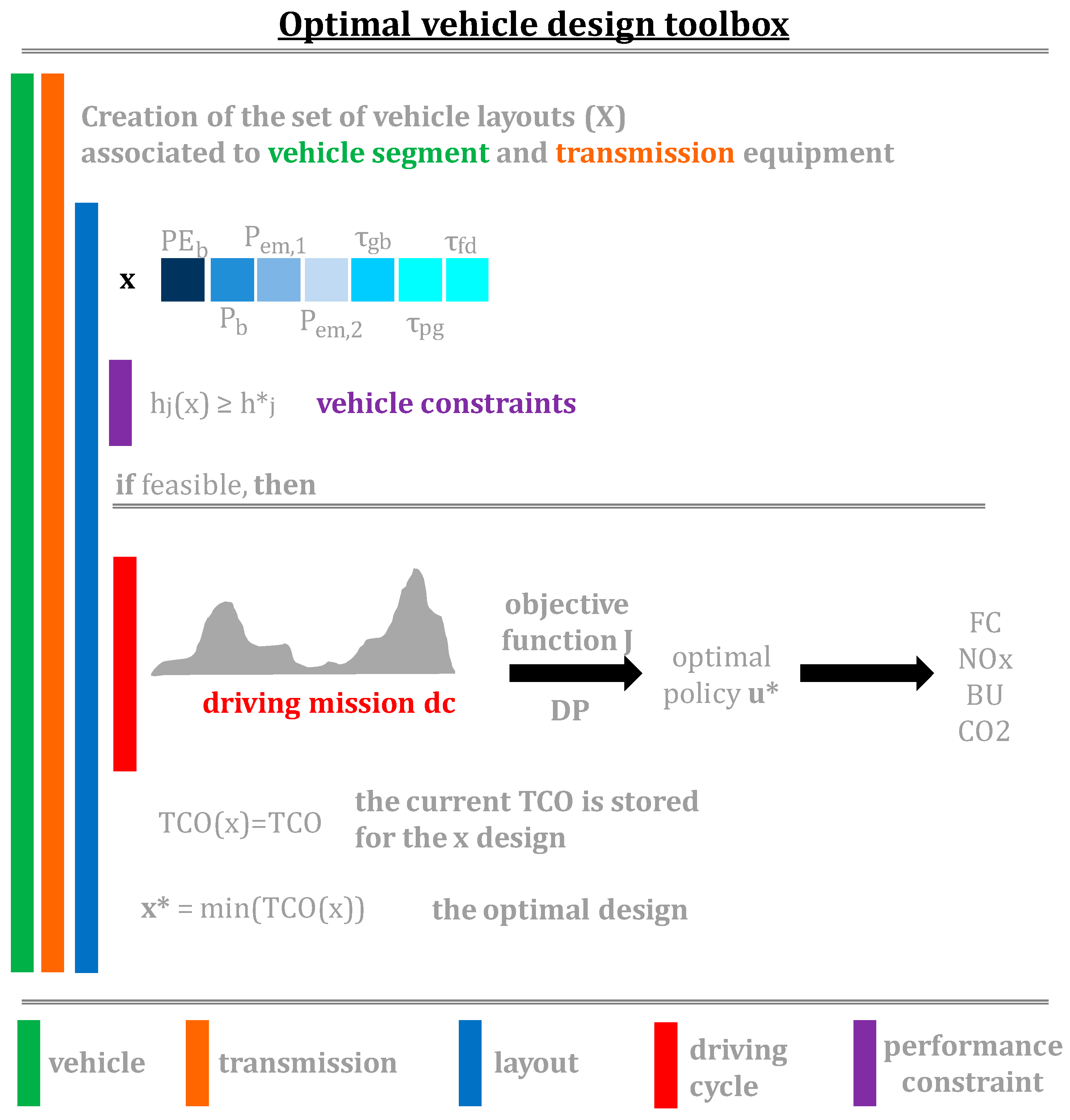
Figure 3.
Vehicle power frequency distribution for the two driving missions.
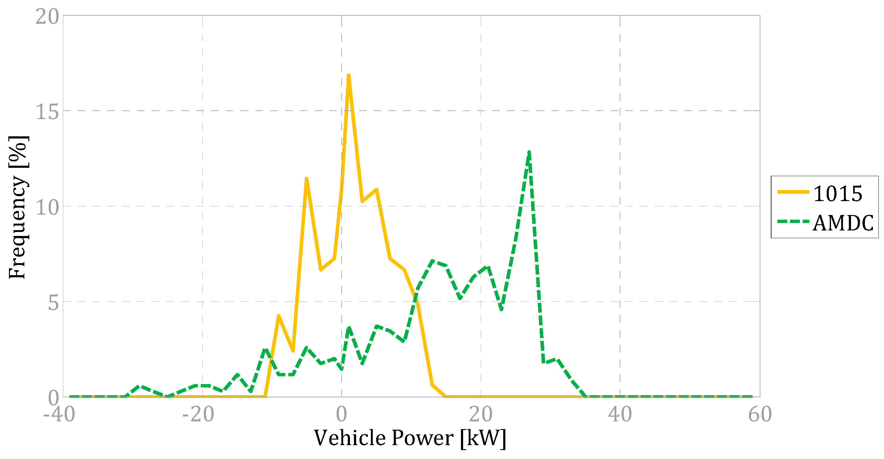
Figure 4.
CO2 emissions (top) and MSRP (bottom) versus the TCO for the feasible designs of the three vehicle segments (a–c) and two layouts (3gTR in yellow, noTR in green), over the 1015 mission.
Figure 4.
CO2 emissions (top) and MSRP (bottom) versus the TCO for the feasible designs of the three vehicle segments (a–c) and two layouts (3gTR in yellow, noTR in green), over the 1015 mission.
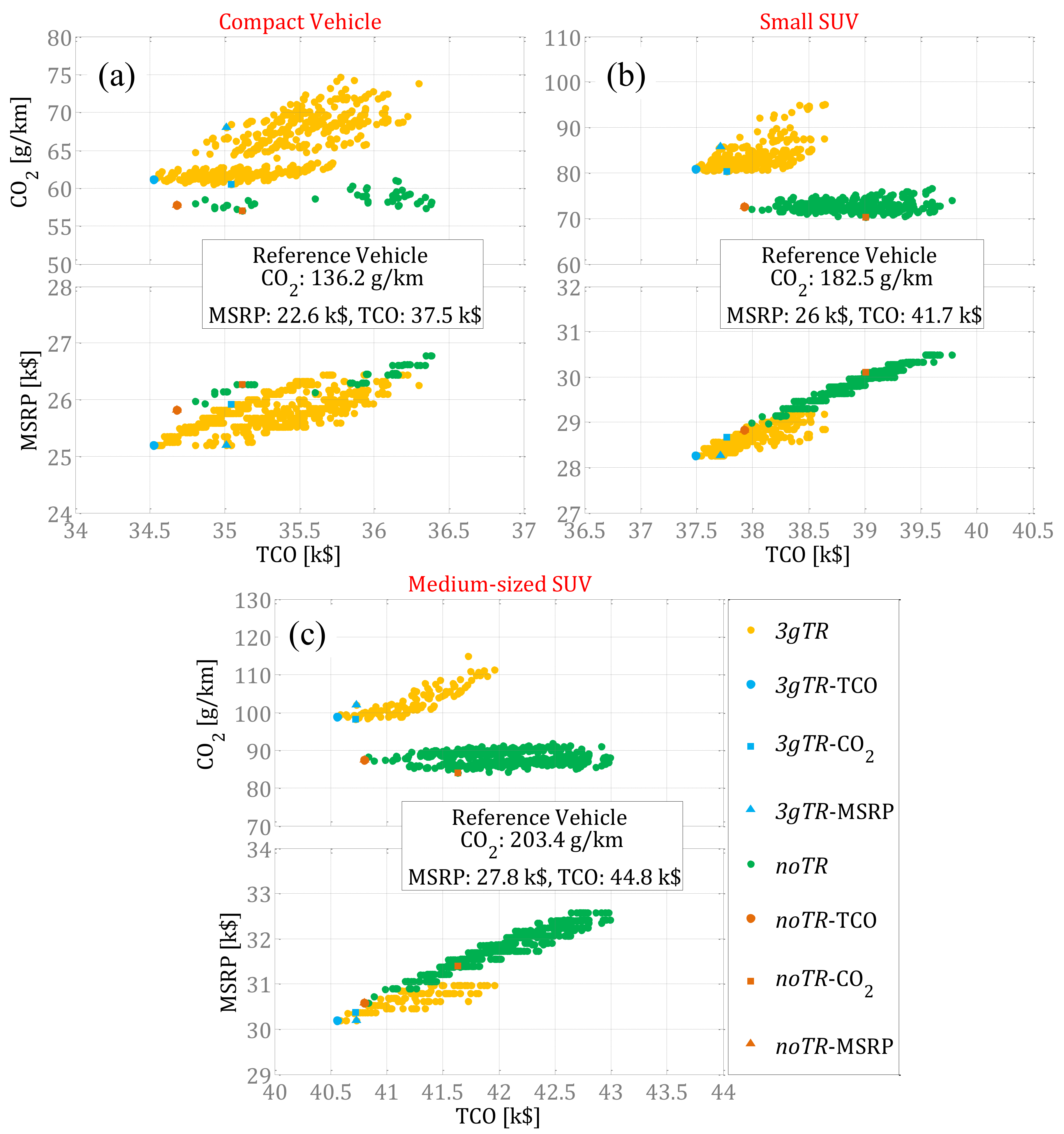
Figure 5.
CO2 (top) and NOx emissions (bottom) versus TCO of the small SUV 3gTR designs over the 1015 (U, yellow dots) and AMDC (H, green dots) missions.
Figure 5.
CO2 (top) and NOx emissions (bottom) versus TCO of the small SUV 3gTR designs over the 1015 (U, yellow dots) and AMDC (H, green dots) missions.

Figure 6.
Cost comparison of the conventional and the hybrid vehicles for the compact segment over the AMDC mission for a short VKT (a) and for the medium-sized SUV segment over the 1015 mission for a long VKT (b).
Figure 6.
Cost comparison of the conventional and the hybrid vehicles for the compact segment over the AMDC mission for a short VKT (a) and for the medium-sized SUV segment over the 1015 mission for a long VKT (b).
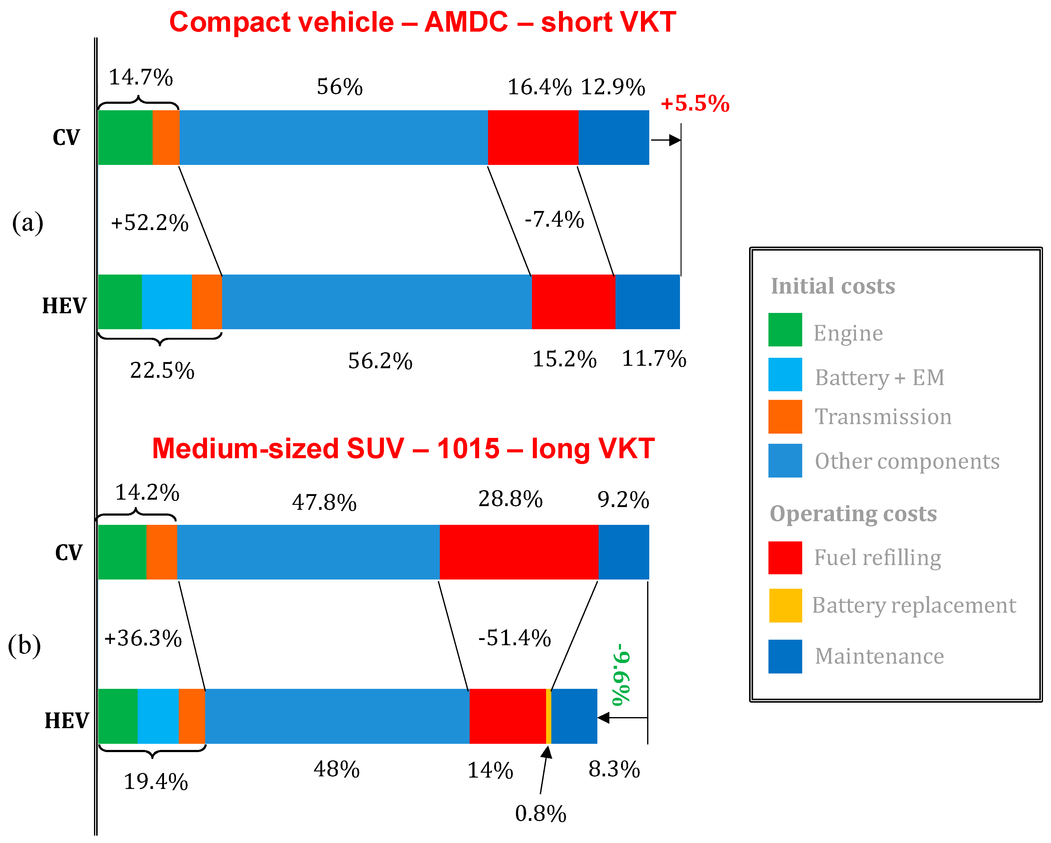
Figure 7.
Cost premium for the compact vehicle (solid yellow line), small SUV (dashed green line) and medium-sized SUV (dashed-dotted cyan line) over their lifetimes, over the 1015 (a,b) and AMDC (c,d) missions for a short (a–c) and long (b–d) VKT.
Figure 7.
Cost premium for the compact vehicle (solid yellow line), small SUV (dashed green line) and medium-sized SUV (dashed-dotted cyan line) over their lifetimes, over the 1015 (a,b) and AMDC (c,d) missions for a short (a–c) and long (b–d) VKT.
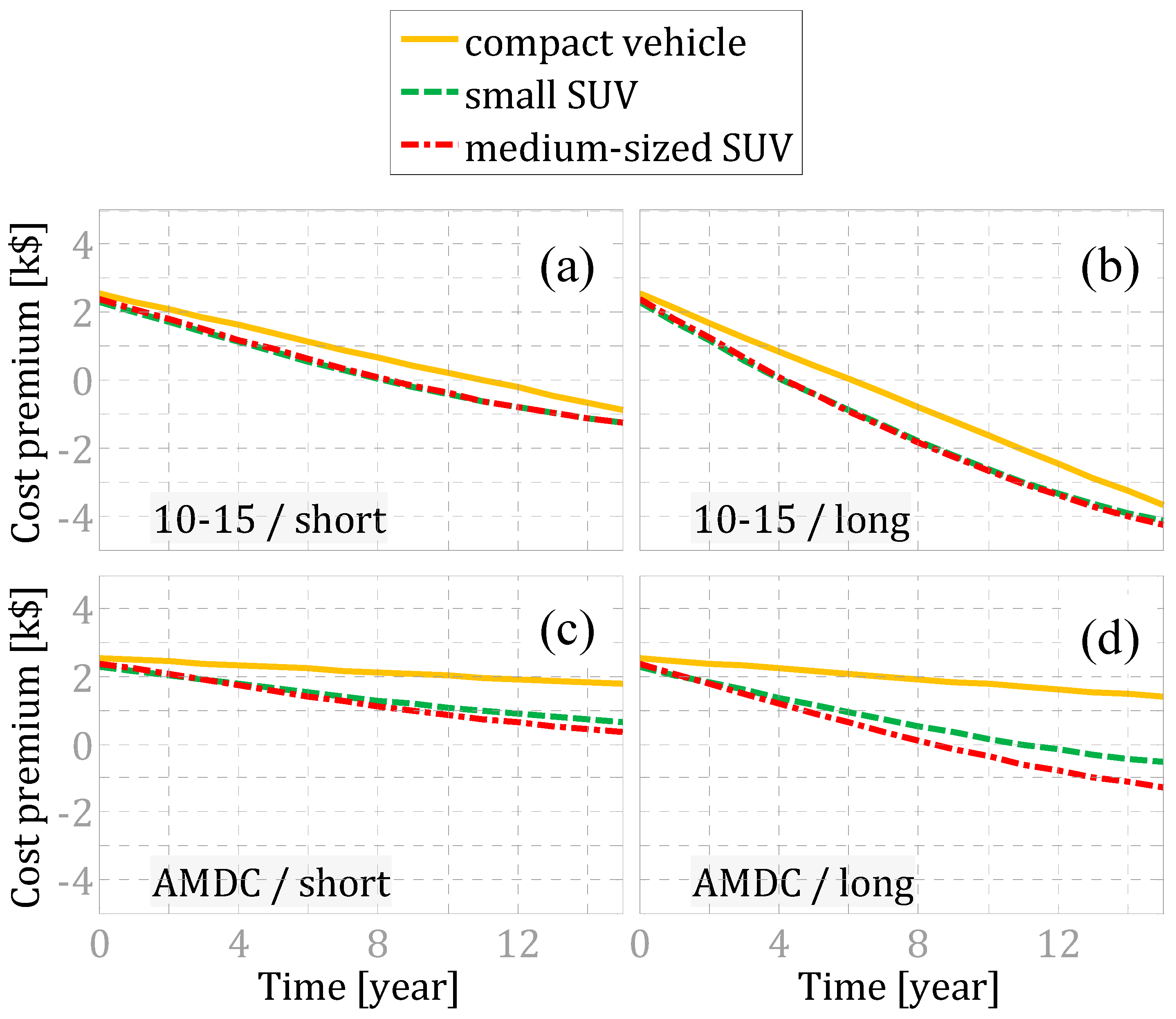
Figure 8.
Cost per day (first column), cost premium (second column) and break-even fuel price (third column) for the compact vehicle (first row), small SUV (second row) and medium-sized SUV (third row), over the 1015 (yellow) and AMDC (cyan) missions for different VKT s.
Figure 8.
Cost per day (first column), cost premium (second column) and break-even fuel price (third column) for the compact vehicle (first row), small SUV (second row) and medium-sized SUV (third row), over the 1015 (yellow) and AMDC (cyan) missions for different VKT s.


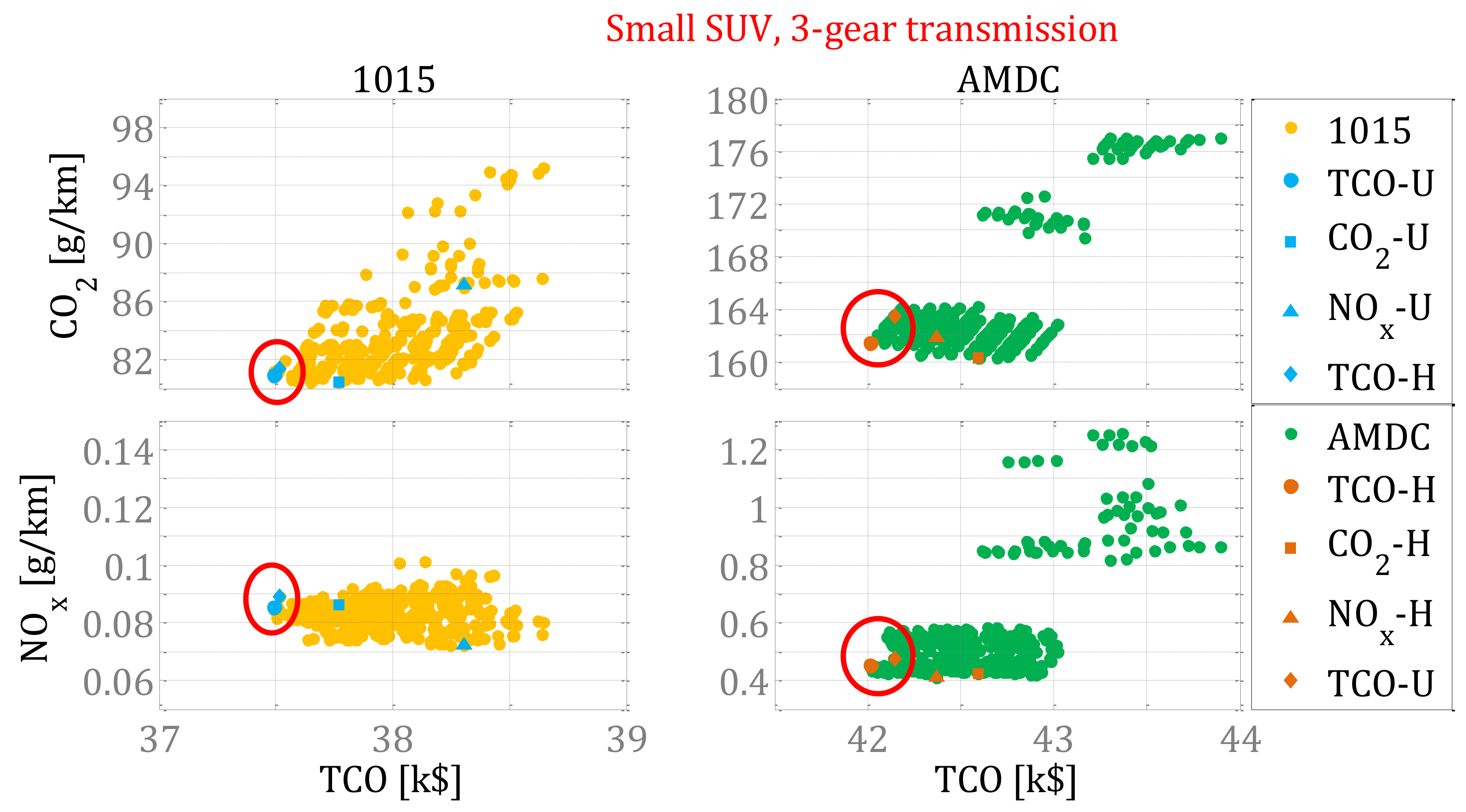
Table 1.
Gear speed ratios, , of the 6-speed and 3-speed transmission devices.
| Transmission | 1 | 2 | 3 | 4 | 5 | 6 |
|---|---|---|---|---|---|---|
| 6-speed | 4.17 | 2.13 | 1.32 | 0.95 | 0.75 | 0.62 |
| 3-speed | 3.06 | 1.53 | 0.765 |
Table 2.
Main specifications of the three diesel engines.
| Engine | Displacement (L) | Max. Power (kW) | Max. Torque (Nm) |
|---|---|---|---|
| D0 | 2.9 | 130 @4000 rpm | 356 @1500 rpm |
| D1 | 1.7 | 97 @3700 rpm | 304 @2400 rpm |
| D2 | 1.3 | 70 @4000 rpm | 206 @1800 rpm |
Table 3.
Engines installed on each vehicle.
| LayoutClass | Compact Vehicle | Small SUV | Medium-Sized SUV |
|---|---|---|---|
| Conventional | D1 | D0 | D0 |
| noTR power-split | D2 | D1 | D1 |
| 3gTR power-split | D2 | D1 | D1 |
Table 4.
Main vehicle specifications of the three vehicle segments.
| Specification | Compact Vehicle | Small SUV | Medium-Sized SUV |
|---|---|---|---|
| chassis mass [kg] | 800 | 1000 | 1270 |
| frontal area [m2] | 2.19 | 2.57 | 2.93 |
| drag resistance coefficient [-] | 0.27 | 0.36 | 0.38 |
| tire radius [m] | 0.317 | 0.359 | 0.367 |
Table 5.
Default sets of the three sub-control variables of the power flow.
| Sub-Control Variable | Value #1 | Value #2 | Value #3 | Value #4 | Value #5 | N |
|---|---|---|---|---|---|---|
| 0.5 | 1 | 1.5 | 3 | |||
| 1 | 1.25 | 1.5 | 1.75 | 2 | 5 | |
| 1 | 0 | 0.25 | 0.5 | 0.75 | 5 |
Table 6.
Performance targets of the three vehicle segments.
| Target | Compact Vehicle | Small SUV | Medium-Sized SUV |
|---|---|---|---|
| Maximum velocity [km/h] | 190 | 190 | 180 |
| Acceleration 0–50 km/h [s] | 4.5 | 4 | 5 |
| Acceleration 0–100 km/h [s] | 11 | 10.5 | 12 |
| Acceleration 65–100 km/h [s] | 5 | 5 | 5.5 |
| Acceleration 80–110 km/h [s] | 5.5 | 5.5 | 6 |
| Tow mass, , [kg] | 1500 | 1500 | 1500 |
| [%] | 20 | 15 | 10 |
Table 7.
Main specifications of the two driving missions.
| T (s) | D (km/h) | (kWh) | (kWh) | (km/h) | (kW) | |
|---|---|---|---|---|---|---|
| 1015 | 660 | 4.17 | 0.37 | −0.20 | 31.65 | 4.71 |
| AMDC | 1068 | 29.36 | 4.33 | −0.59 | 100.1 | 17.74 |
Table 8.
Mass (kg) and performances of the three layouts (conventional and hybrid) for the three vehicle segments.
Table 8.
Mass (kg) and performances of the three layouts (conventional and hybrid) for the three vehicle segments.
| Class | Layout | Mass (kg) | Power-To-Mass (W/kg) | 0–50 km/h Time (s) | 0–100 km/h Time (s) |
|---|---|---|---|---|---|
| Compact | CV | 1345 | 62.89 | 4.15 | 10.05 |
| noTR | 1265.1 | 69.7 | 4.45 | 10.7 | |
| 3gTR | 1266.9 | 58.1 | 3.35 | 9.8 | |
| Small SUV | CV | 1630 | 69.9 | 3.45 | 9.3 |
| noTR | 1525.7 | 80.7 | 4 | 10.4 | |
| 3gTR | 1531.8 | 66.6 | 3.25 | 9.1 | |
| Medium SUV | CV | 1900 | 59.9 | 4 | 10.95 |
| noTR | 1795.7 | 63.1 | 4.85 | 11.95 | |
| 3gTR | 1805.2 | 56.6 | 3.5 | 10.3 |
Table 9.
Reduction in CO2 emissions (first column), TCO (second column) and increment in MSRP (third column) of the six designs of the three vehicle segments, with respect to the conventional vehicle.
Table 9.
Reduction in CO2 emissions (first column), TCO (second column) and increment in MSRP (third column) of the six designs of the three vehicle segments, with respect to the conventional vehicle.
| CO2 (%) | TCO (%) | MSRP (%) | ||
|---|---|---|---|---|
| Compact vehicle | 3gTR-TCO | 55.1 | 9.6 | 11.2 |
| 3gTR-CO2 | 55.5 | 8.3 | 14.4 | |
| 3gTR-MSRP | 50.0 | 8.3 | 11.2 | |
| noTR-TCO | 57.6 | 9.2 | 14.0 | |
| noTR-CO2 | 58.1 | 8.0 | 16.0 | |
| noTR-MSRP | 57.6 | 9.2 | 14.0 | |
| Small SUV | 3gTR-TCO | 55.7 | 10 | 8.8 |
| 3gTR-CO2 | 55.9 | 9.3 | 10.4 | |
| 3gTR-MSRP | 53 | 9.5 | 8.8 | |
| noTR-TCO | 60.2 | 8.9 | 11 | |
| noTR-CO2 | 61.5 | 6.3 | 15.9 | |
| noTR-MSRP | 60.2 | 8.9 | 11 | |
| Medium-sized SUV | 3gTR-TCO | 51.4 | 9.5 | 8.6 |
| 3gTR-CO2 | 51.7 | 9.1 | 9.2 | |
| 3gTR-MSRP | 50 | 9.1 | 8.6 | |
| noTR-TCO | 57 | 8.9 | 9.9 | |
| noTR-CO2 | 58.7 | 7.1 | 12.9 | |
| noTR-MSRP | 57 | 8.9 | 9.9 |
Table 10.
Reduction in CO2 emissions (1st column), increment in TCO (2nd column) and MSRP (3rd column), CBF (4th column) and PBF (5th column) of the five designs for the three segments, with respect to .
Table 10.
Reduction in CO2 emissions (1st column), increment in TCO (2nd column) and MSRP (3rd column), CBF (4th column) and PBF (5th column) of the five designs for the three segments, with respect to .
| CO2 | TCO | MSRP | CBF | PBF | ||
|---|---|---|---|---|---|---|
| (%) | (%) | (%) | ($/(g/km)) | ($/(g/km)) | ||
| Compact vehicle | 3gTR-CO2 | 0.9 | 1.5 | 2.9 | 1290.3 | 916.3 |
| 3gTR-MSRP | −11.4 | 1.4 | 0 | - | −70.2 | |
| noTR-TCO | 5.4 | 0.5 | 2.5 | 188.9 | 46.5 | |
| noTR-CO2 | 6.7 | 1.7 | 4.3 | 264.4 | 145.7 | |
| noTR-MSRP | 5.4 | 0.5 | 2.5 | 188.9 | 46.5 | |
| Small SUV | 3gTR-CO2 | 0.7 | 0.7 | 1.4 | 770 | 528.5 |
| 3gTR-MSRP | −5.9 | 0.6 | 0 | 0 | −46.4 | |
| noTR-TCO | 10.2 | 1.2 | 2 | 68.4 | 52.8 | |
| noTR-CO2 | 13.2 | 4.1 | 6.5 | 172.5 | 142 | |
| noTR-MSRP | 10.2 | 1.2 | 2 | 68.4 | 52.8 | |
| Medium-sized SUV | 3gTR-CO2 | 0.6 | 0.4 | 0.6 | 288.6 | 271.2 |
| 3gTR-MSRP | −3.2 | 0.4 | 0.0 | 0.0 | −52.3 | |
| noTR-TCO | 11.6 | 0.6 | 1.2 | 32.7 | 21.0 | |
| noTR-CO2 | 15.0 | 2.6 | 4.0 | 80.6 | 72.5 | |
| noTR-MSRP | 11.6 | 0.6 | 1.2 | 32.7 | 21.0 |
Table 11.
The tuned k coefficients of the TCO and CO2 correlations.
| k | 0 | 1 | 2 | 3 | 4 | 5 | 6 | 7 |
|---|---|---|---|---|---|---|---|---|
| TCO | 38535 | −24.37 | 17.95 | 43.73 | 0 | −80.31 | −34.24 | −154.2 |
| CO2 | 104.34 | −0.0023 | −0.0415 | 0.142 | 0 | −2.453 | −0.683 | −2.568 |
Table 12.
Design component specifications and actual performance of the six optimized vehicles.
| Specification | Compact Vehicle | Small SUV | Medium-Sized SUV | |||
|---|---|---|---|---|---|---|
| 3-Gear transmission | ✓ | ✗ | ✓ | ✗ | ✓ | ✗ |
| Maximum engine power [kw] | 69 | 69 | 96 | 96 | 96 | 96 |
| Battery P/E ratio [W/Wh] | 30 | 30 | 30 | 30 | 30 | 30 |
| Maximum battery power [kw] | 20 | 40 | 25 | 50 | 30 | 50 |
| Maximum EM1 power [kw] | 10 | 25 | 10 | 25 | 10 | 35 |
| Maximum EM2 power [kw] | 15 | 20 | 20 | 30 | 20 | 20 |
| GB speed ratio [-] | 2 | 2 | 2.5 | 2.5 | 2 | 2.5 |
| PG speed ratio [-] | 4.5 | 4 | 4.5 | 4.5 | 5 | 4.5 |
| FD speed ratio [-] | 5 | 4 | 5.5 | 4.5 | 5.5 | 4.5 |
| Maximum velocity [km/h] | 201.5 | 191 | 197.5 | 191.5 | 185.5 | 180 |
| Acceleration 0–50 [s] | 3.35 | 4.45 | 3.25 | 4 | 3.5 | 4.85 |
| Acceleration 0–100 [s] | 9.8 | 10.7 | 9.1 | 10.4 | 10.3 | 11.9 |
| Acceleration 65–100 [s] | 4.9 | 4.5 | 4.4 | 4.7 | 5.2 | 5.2 |
| Acceleration 80–110 [s] | 5.2 | 4.2 | 4.7 | 4.7 | 5.5 | 5.7 |
| Tow mass [kg] | 1600 | 3250 | 1750 | 3050 | 1750 | 2350 |
| [%] | 63 | 36 | 61 | 42 | 48 | 33 |
Table 13.
Increment in TCO, CO2 and NOx emissions for different objective functions over the 1015 mission, with respect to the default J function, for the compact vehicle with no transmission.
Table 13.
Increment in TCO, CO2 and NOx emissions for different objective functions over the 1015 mission, with respect to the default J function, for the compact vehicle with no transmission.
| Oriented Optimization | TCO [%] | CO2 [%] | NOx [%] | ||
|---|---|---|---|---|---|
| FC | 0 | 0 | 1.6 | −11.5 | 120.7 |
| FC-BU | 0 | 0.2 | −0.3 | −7.3 | 35 |
| FC-BU | 0 | 0.4 | −0.3 | −4.4 | 38.3 |
| FC-BU | 0 | 0.5 | −0.2 | −1.9 | 37.5 |
| FC-BU | 0 | 0.6 | −0.1 | −0.7 | 31.8 |
| FC-BU | 0 | 0.8 | 0.4 | 5.9 | 30.9 |
| FC-BU-NOx | 0.1 | 0.4 | 0 | −0.1 | −3.9 |
| FC-BU-NOx | 0.2 | 0.4 | 0.4 | 2.9 | −20.5 |
| NOx | 1 | 0 | 2.6 | 0.64 | −36.6 |
© 2018 by the authors. Licensee MDPI, Basel, Switzerland. This article is an open access article distributed under the terms and conditions of the Creative Commons Attribution (CC BY) license (http://creativecommons.org/licenses/by/4.0/).
Share and Cite
MDPI and ACS Style
Finesso, R.; Misul, D.; Spessa, E.; Venditti, M. Optimal Design of Power-Split HEVs Based on Total Cost of Ownership and CO2 Emission Minimization. Energies 2018, 11, 1705. https://doi.org/10.3390/en11071705
AMA Style
Finesso R, Misul D, Spessa E, Venditti M. Optimal Design of Power-Split HEVs Based on Total Cost of Ownership and CO2 Emission Minimization. Energies. 2018; 11(7):1705. https://doi.org/10.3390/en11071705
Chicago/Turabian StyleFinesso, Roberto, Daniela Misul, Ezio Spessa, and Mattia Venditti. 2018. "Optimal Design of Power-Split HEVs Based on Total Cost of Ownership and CO2 Emission Minimization" Energies 11, no. 7: 1705. https://doi.org/10.3390/en11071705
Note that from the first issue of 2016, this journal uses article numbers instead of page numbers. See further details here.