The Application of Heterogeneous Information Fusion in Misalignment Fault Diagnosis of Wind Turbines

1
School of Mechanical, Electronic and Control Engineering, Beijing Jiaotong University, Beijing 100044, China
2
School of Electrical and Electronic Engineering, The University of Manchester, Manchester M13 9PL, UK
*
Author to whom correspondence should be addressed.
Energies 2018, 11(7), 1655; https://doi.org/10.3390/en11071655
Submission received: 28 May 2018
/
Revised: 19 June 2018
/
Accepted: 20 June 2018
/
Published: 26 June 2018
Abstract
:The misalignment of the drive system is one of the important factors causing damage to gears and bearings on the high-speed output end of the gearbox in doubly-fed wind turbines. How to use the obtained information to determine the types of the faults accurately has always been a challenging problem for researchers. Under the restriction that only one kind of signal is used in the current wind turbine fault diagnosis, a new method based on heterogeneous information fusion is presented in this paper. The collected vibration signal, temperature signal, and stator current signal are used as original sources. Their time domain, frequency domain and time-frequency domain information are extracted as fault features. Taking into account the correlation between the features, t-distributed Stochastic Neighbor Embedding (t-SNE) is used to reduce the dimensionality of the original combinations. Then, the fusion features are put into the Least Square Support Vector Machine (LSSVM), which is optimized by artificial bee colony (ABC) algorithm. The simulation tests show that this method has higher diagnostic accuracy than other methods.
1. Introduction
To cope with the global warming trend, most countries have reduced carbon emissions year by year as one of the requirements of domestic economic and social development [1]. As a clean energy, wind power is superior to hydropower and nuclear power in energy conservation, and environmental and ecological protection [2]. In recent years, wind power has been developed rapidly in various countries, and the installed capacity has increased year after year [3].
Wind farms are generally located in remote areas with abundant wind resources, and the working environment is complex. The probability of failure of various components in wind turbines is relatively large [4]. If a key component of the unit fails, it will damage the equipment and even cause the unit to stop at once, resulting in huge economic losses. Faults of wind turbines include blade failure, transmission system failure, generator failure, and tower failure. Among them, misalignment of transmission system is one of the most common failures. In practice, there are many reasons that can cause the wind turbine transmission system to be misaligned, such as bearing eccentricity, installation error, misalignment of the coupling, etc. [5]. The drive system of a doubly-fed wind turbine is an important transmission device to connect the turbine and the generator. The misalignment of the transmission system will inevitably cause vibration of the wind turbines and endanger the reliability of the gears and bearings. Therefore, it is important to monitor and diagnose the misalignment of the transmission system in doubly-fed wind turbines [6].
Currently, methods of fault diagnosis for rotating machinery drive systems are mainly based on oil analysis [7], noise monitoring [8], vibration monitoring [9], and stator current analysis [10]. Though the content of the wear debris in the lubricating oil can be detected and analyzed to determine the degree of some failure, it is inconvenient to extract the grinding debris in the lubricating oil of the wind turbines at a high-altitude [11]. The principle of fault diagnosis based on noise is that when a fault occurs, the mechanical noise will increase. However, the wind turbine is a system with a long transmission chain, and the noise interference is very severe [12]. The diagnostic based on noise is easily affected by the external environment and the diagnosis results will be inevitably affected [13]. Therefore, for the fault diagnosis of large-scale rotary mechanical transmission systems such as wind turbines, vibration-based monitoring and stator current-based analysis are the two most commonly used methods currently [14]. On the other hand, according to the feedback from wind farms, misalignment is a common failure of wind turbines [15]. Once misalignment occurs, the high-speed drive shafts are subject to greater friction and will generate more heat, which can easily lead to the destruction of lubricating oils and the appearance of gear gluing phenomenon. Hence use the temperature information to diagnose the wind turbines is also a good method [16,17].
The above mentioned studies are all based on single information such as vibration, stator current, or temperature to perform wind turbine fault diagnosis. In recent years, there are also some references to fuse signals to diagnosis. For example, reference [18] had proposed a method to extract the characteristics of gearbox rotation speed and temperature monitoring data through kernel principle component analysis (KPCA), then put them into relevance vector machine (RVM) for training. Reference [19] considered gearbox vibration signal, temperature signal and lubrication signal as original sources, and used principal component analysis to reduce the dimensionality. The generator stator current of the wind turbines is very convenient to obtain, and the feasibility and correctness of using it to diagnose misalignment is proved in literature [20]. At the same time, in literature [21], the vibration signal was used to diagnose misalignment effectively; in literature [22], the temperature was used in fault diagnosis. Therefore in this paper, the vibration signal, temperature signal, and stator current signal are regarded as the original sources, and their time domain, frequency domain, and time-frequency domain indexes are extracted as fault features. The t-distributed stochastic neighbor embedding (t-SNE) is used to combine them. The fusing features are put into the least square support vector machine (LSSVM), which is optimized by artificial bee colony algorithm. Simulation tests show that this method has higher diagnostic accuracy than other parameter optimization models and information fusion methods.
2. The Related Theory
2.1. The Concept of Information Fusion
With the development of society, mechanical systems have become more and more complicated. If only one single sensor is used to obtain information and make judgments, it is very unreasonable and sometimes may lead to misjudgment [23]. In this situation, information fusion technology came into being. It is a technique of comprehensive processing for multidimensional information, which makes up for the insufficiency of traditional relying on single information [24].
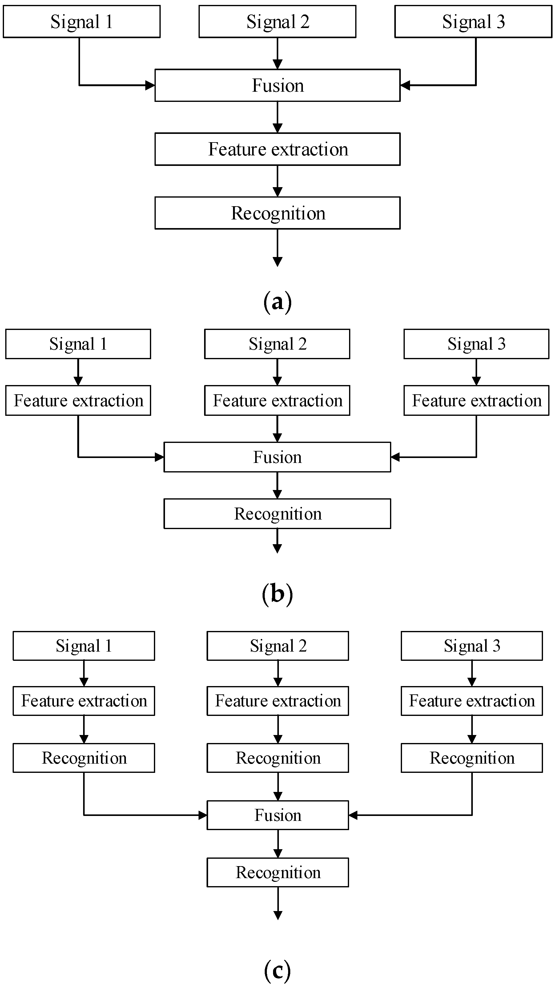
The information fusion mainly has three levels of integration, which are data level fusion, feature level fusion, and decision level fusion [25,26].
- Data Level Fusion. Also called pixel level fusion. It is a comprehensive analysis of raw information. In this level of fusion, information loss is small, but the calculation is large. Real-time and fault tolerance are poor, and the level of integration is low. Because of the presence of redundant information, it may affect the diagnostic accuracy. Data level fusion is generally limited to the same type of sensor information.
- Feature Level Fusion. The data from multiple sensors must be preprocessed, forming feature vectors, which were fused to get the joint feature vector. Feature level fusion is more real-time than data level fusion. If the selected algorithm is reasonable, the elimination of redundant information will improve the accuracy of diagnosis.
- Decision Level Fusion. Each sensor’s processing system has completed its decision-making or classification tasks before fusion. Optimal decisions are made based on certain criteria and the credibility of decisions through fusion. Decision level fusion is the highest level of fusion. Its real-time performance and fault tolerance are good, but information loss is large and more complicated algorithms are needed.
The structures of the three fusions are shown in Figure 1.
In this paper, the vibration signal, the temperature signal and the stator current signal are used as the original sources to achieve feature level fusion.
2.2. Dimension Reduced Feature Fusion Algorithm
Heterogeneous information is highly complementary, and the fusion information generated by it is more practical. Therefore, using heterogeneous information fusion for fault diagnosis can often achieve better diagnostic results than similar information fusion. However, the more signals there are, the higher dimension of the constructed feature vectors is, which not only increases the computational complexity, but also brings difficulties to the intuitive fault diagnosis [27]. In order to make better use of various kinds of information and get good diagnostic results, dimensionality reduction methods are usually used. The common dimensionality reduction methods include: linear mapping methods such as PCA, Fisher discriminant analysis (FDA); non-linear kernel mapping methods such as kernel principal component analysis (KPCA), kernel Fishers discriminant analysis (KFDA); and manifold learning methods such as Laplacian eigenmaps (LE), local linear embedding (LLE), isometric mapping (ISOMAP), local preserved projection (LPP), local tangent space alignment (LTSA), and stochastic neighbor embedding (SNE). Many scholars have applied the manifold learning method to machinery fault diagnosis, and achieved good results. For example, Wang guode et al. used the LLE algorithm to reduce the dimensionality of the constructed high-dimensional vectors [28]; Liu hui improved the effectiveness and robustness of the ISOMAP algorithm [29]; Li feng et al. proposed a dimension reduction model based on LTSA and applied it to fault diagnosis of deep groove ball bearings [30]. Although the manifold learning algorithm has been applied in the field of mechanical fault diagnosis, some problems such as non-linear data crowding, which is not clear in low-dimensional manifold expression, still exist [31]. So in this paper, aiming at the above mentioned deficiencies, the t-distributed stochastic neighbor embedding (t-SNE) algorithm is mainly studied and applied to the misalignment diagnosis of wind turbines.
t-SNE [32] is an improved dimension reduction visualization method proposed by Maaten and Hinton in 2008 based on SNE. The SNE algorithm is a nonlinear dimension reduction method based on the conditional probability theory [33], which can reduce a high-dimensional data set to a two-dimensional or three-dimensional data set that can be graphically displayed. The SNE algorithm has the problems of optimization difficulty in value equations and crowding problems in low-dimensional manifolds. The t-SNE is improved on the basis of SNE. The symmetry value equation and t-distribution are used to calculate the similarity between two points in low-dimensional space instead of Gaussian distribution to solve the problems of low-dimensional space crowding and parameter optimization.
The specific principle of the t-SNE learning algorithm is [32]: The t-SNE treats coordinates in low dimensions as t-distributions, while SNE treats sample distributions in high and low dimensions as Gaussian distributions. The advantage of this approach is to increase the distance between clusters with large distances further, thus solving the crowding problem. Compared with SNE, t-SNE introduces a strong rebound force to make the distance between the low-dimensional dissimilar data increase. The strength of the force between dissimilar data is proportional to the distance in the low-dimensional space. Thus it is finally realized that data with small distances in low-dimensional space represents data with certain similarity in high-dimensional space, and data with large distance in low-dimensional space represents data dissimilar in high-dimensional space.
Its implementation steps are as follows:
- (1)
- Define a high-dimensional data set:
- (2)
- Compute the complexity parameter of the value equation :where, is the conditional probability of data points (other than ) with respect to , is the conditional probability of high-dimensional data, is the joint probability density in the high-dimensional space, and is the joint probability density in the low-dimensional mapping space.
- (3)
- Define the optimization parameters: the number of iterations T, the learning rate η, the momentum factor at the tth (t ≤ T) iteration . The value equation c is learned by the gradient descent method, and the low-dimensional mapping of the high-dimensional data is finally obtained:where, and are the mapping of the high-dimensional data and in the low-dimensional space.
In order to speed up the optimization process and prevent trapping into local minima, a relatively large momentum condition is imposed on the descent process. The current gradient value is summed to the previous gradient value each iteration and then decays exponentially to determine the coordinates of the low-dimensional data. The momentum formula is as the following:
where, is the data in the low-dimensional space.
2.3. Fault Diagnosis Method and Parameters Optimization
Support vector machine (SVM) can well solve the problems of nonlinearity, high dimensionality, and local minimum [34], but it also has certain limitations, such as the blindness of parameter determination, and the solution will become more complex as the training samples increase [35]. In order to solve the shortcomings of SVM, many scholars conducted research and proposed solutions. Among them, the widely used method is the least square support vector machine (LSSVM) [36].
LSSVM also follows the principle of minimizing structural risk. The equality constraints are used to replace the inequality constraints in SVM. Linear equations instead of quadratic programming are used in the solution to the optimization problem. At the same time, the deviation of empirical risk is changed to a quadratic. The complexity has been reduced, but the operation speed is higher than SVM [37].
When using a radial basis kernel function, the parameters of LSSVM are few, and only include the regularization parameter C and the kernel width σ [38]. The parameters of the LSSVM have a very important role in the performance of the algorithm. Different parameters are selected, and different classifications may be obtained. How to choose the appropriate regularization parameter C and kernel width σ has no clear theoretical method at present. Trial method is usually adopted, which not only takes time and effort, but also the solution of the optimization problem is influenced by subjective factors, so the problem of parameter selection is one of the hotspots of research [38]. The commonly used selection methods are: cross validation method, grid search method and intelligent optimization algorithm.
The swarm intelligence algorithm is an intelligent optimization algorithm proposed in recent years. It simulates the behavior of animals in groups, and utilizes information interaction and cooperation among individuals to achieve optimization. The swarm intelligence algorithm is easy to implement and has high efficiency, so it has rapidly become a research hotspot in the optimization field. Many scholars apply the swarm intelligence algorithm to the parameter optimization of the LSSVM [39].
The swarm intelligence algorithm mainly includes the genetic algorithm, artificial immune algorithm, particle swarm optimization, artificial fish swarm algorithm, artificial bee colony algorithm, and so on. Among them, the artificial bee colony (ABC) algorithm is a swarm intelligence optimization algorithm proposed in recent years. It has many advantages such as good optimization ability, less control parameters, and is simple, flexible, and easy to implement. Research shows that the optimization performance of the artificial bee colony algorithm is better than that of the genetic algorithm, differential evolution algorithm, and particle swarm algorithm [40]. The optimized SVM by artificial bee colony algorithm is better than that by genetic algorithm, ant colony algorithm and standard particle swarm optimization [41]. Therefore, the artificial bee colony algorithm will be used to optimize parameters in this paper.
The artificial bee colony algorithm [42] imitates the collecting honey process of natural bees. Each food source corresponds to a collecting bee at the time of initialization. The location of the food source represents a solution to the optimization problem, and the quality or fitness of each solution corresponds to the amount of nectar of the food source. The specific principle is: First, initialize a population containing solutions. Each solution is a D-dimensional column vector, where D represents the number of optimization parameters. The collecting bees search the neighborhood of the food source, to find new food sources and compare them with the old ones, adopting greed principle to select food sources with better fitness values. Each collecting bee returns to the hive after completing a neighborhood search and updating the food source, and shares the food source information (position and fitness value of solution) with the observing bees through dancing. Observing bees select the food source according to the information of collecting bees, then use the greedy criterion to search for neighbors, and select the food source with higher fitness. The observing bee selects the food source according to the following formula:
where is the probability of observing the bee’s choice of food source, and is the fitness value of the ith solution.
New food source location is generated according to Equation (7):
where, , , , which is a random number used to control the neighborhoods range of . The closer to the optimal solution, the smaller the neighborhood range is.
If a food source has not been improved after N cycles, then the solution will be abandoned. The collecting bee in this position is converted to a detecting bee, and then a new solution is randomly generated according to Equation (8):
So, the artificial bee colony algorithm includes four steps:
(1) The observing bees find the global optimization of the food source according to Equation (6);
(2) The collecting bees and the observing bees perform the neighborhood searching according to Equation (7);
(3) All bees compare the old food source with the new food source, and select the better food source with greedy criterion;
(4) The detecting bees provide random solution to produce food sources according to Equation (8).
Figure 2 shows the implementation of artificial bee colony algorithm.
3. Signal Acquisition and Feature Extraction
3.1. Signal Acquisition
The premise of the fault diagnosis for the wind turbines is the acquisition of effective fault information. The methods of obtaining misalignment information can be mainly divided into two types:
(1) Obtain the misaligned information by collecting data on-site or by creating faults on test bench. For example, in literature [43], the vibration test system was used to measure the faulty wind turbine. Relevant time domain and frequency domain analysis were carried to extract the double frequency feature of the high speed end when misalignment occurred, which provided the basis for misalignment fault diagnosis of wind turbines. However, the running time of wind turbines is relatively short. Therefore, the operational data and experience of the wind turbines used in misalignment diagnosis are relatively scarce. Sometimes, it is difficult to analyze the causes of the defects. For example, it may not be clear whether the generator is misaligned, unbalanced, loose parts, or shaft bent. In view of this situation, some scholars use certain physical models to create faults to conduct fault diagnosis research [44]. However, this is sometimes destructive, and the faults produced are relatively single. The cost of the experiment is too high.
(2) Obtain the misaligned information by using simulation software. For example, Liu Rongzhen and Hu Shushan [45] analyzed the mechanism of misalignment of gear couplings, and built a virtual prototype model of the wind turbine system through embedded Hertz contact theory. The simulation analysis of the misalignment of the gear coupling under multi-operating conditions showed the evolution with the change of misalignment.
Simulating the misalignment of wind turbines by software is a cost-effective method. This paper analyzed the misalignment faults based on the models of wind turbines established by ADAMS 2013, MATLAB R2014a and Ansys 17.0. The three-dimensional (3D) model of 1.5 MW wind turbine is established using Solidworks, and the model is then imported into ADAMS 2013, where the Marker point was moved according to the type and degree of misalignment. Misalignment failures can be simulated due to the eccentric mass excitation generated by the center of mass deviating from the center of rotation (details in literature [46]). The wind turbine models and its control system are established by MATLAB (details in literature [47]). The vibration and stator current can be extracted from the models. Also, the high-speed gear shaft and the main shaft of the generator are introduced into Hypermesh to divide the grid. After reaching the required precision, the model is imported into Ansys Workbench to get the corresponding temperature signals (details in literature [48]). The correctness of the models have been verified in the literature [46,47,48]. This method is simpler and more efficient to operate, and the simulation process is faster.
3.2. Feature Extraction
3.2.1. Time Domain Feature Extraction
The signal of the transmission system (assuming the signal is a discrete sequence of finite length ) contains information of its working status, so some representative time domain indexes can be selected as the fault features. Changes of them can help determine if faults happened and what type of misalignment had occurred. The time domain indexes of the signal include dimensional and dimensionless indexes [49].
(1) Dimensional indexes. The commonly used dimensional indexes include: the variance, the square root amplitude, the root mean square (RMS) value, the standard deviation and the kurtosis. Their calculations are:
(2) Dimensionless indexes. The dimensionless indexes are insensitive to the changes of the amplitude and frequency of the signal, that is, they are not related to the working conditions of the unit. The kurtosis index, waveform index, peak index, pulse index and margin index are commonly used dimensionless indexes. Their calculations are:
Kurtosis index:
Waveform index:
where, the average amplitude is: .
Peak index:
where represents the peak.
Pulse index:
Margin index:
3.2.2. Frequency Domain Feature Extraction
For complex signals, time domain analysis can extract very limited information. Therefore, the time domain signal is often transformed to the frequency domain by mathematics, revealing the frequency composition of the signal, thereby extracting more information of the signal [50].
For a finite-length discrete sequence , assuming the sampling frequency is , the commonly used frequency domain indexes are as the following.
where, is the power spectrum of the discrete signal, , , is the angular frequency.
3.2.3. Time-Frequency Feature Extraction
In this paper, in terms of vibration signals, the method of image extension is used to improve Empirical Mode Decomposition (EMD) (see literature [21]), and the energy entropy of the signal is extracted as the time-frequency domain index after the Improved Empirical Mode Decomposition (hereinafter referred to as IEMD). The energy entropy is defined as follows [21]:
Assume:
where , is the amplitude of each discrete point.
The expression formula of IEMD energy entropy is:
For stator current signals, after performing four-layer dual-tree complex wavelet transform (DTCWT) on them, the five sub-band signals are obtained. They are then individually reconstructed to obtain five sub-band reconstruction signals [20]. The energy entropy, sample entropy, and spectral kurtosis of the five sub-band reconstruction signals are extracted.
The energy entropy formula is Equation (26), mentioned above.
When the sequence length is finite, the sample entropy of the time series is:
where m is the dimension of the vector , r is the given threshold, and is the average of the two vectors maximum distance.
The spectral kurtosis formula is:
where, is the second-order spectral moment of the signal, is the fourth-order spectral moment of the signal.
3.2.4. Three Signals Feature Extraction
Table 1 shows a 21-dimensional mixed feature library of vibration signals in the time, frequency, and time-frequency domain.
This paper selects the gearbox tooth temperature T1 and the gearbox rotor shaft temperature T2 as the characteristic values of the temperature signals. Construct a two-dimensional feature vector of the temperature signals: X = [T1, T2].
Table 2 is a 29-dimensional mixed feature library of stator current signals in the time, frequency and time-frequency domain.
Therefore, the feature vectors of the three types of information are 52-dimensional.
4. The Fault Diagnosis Implementation and Results
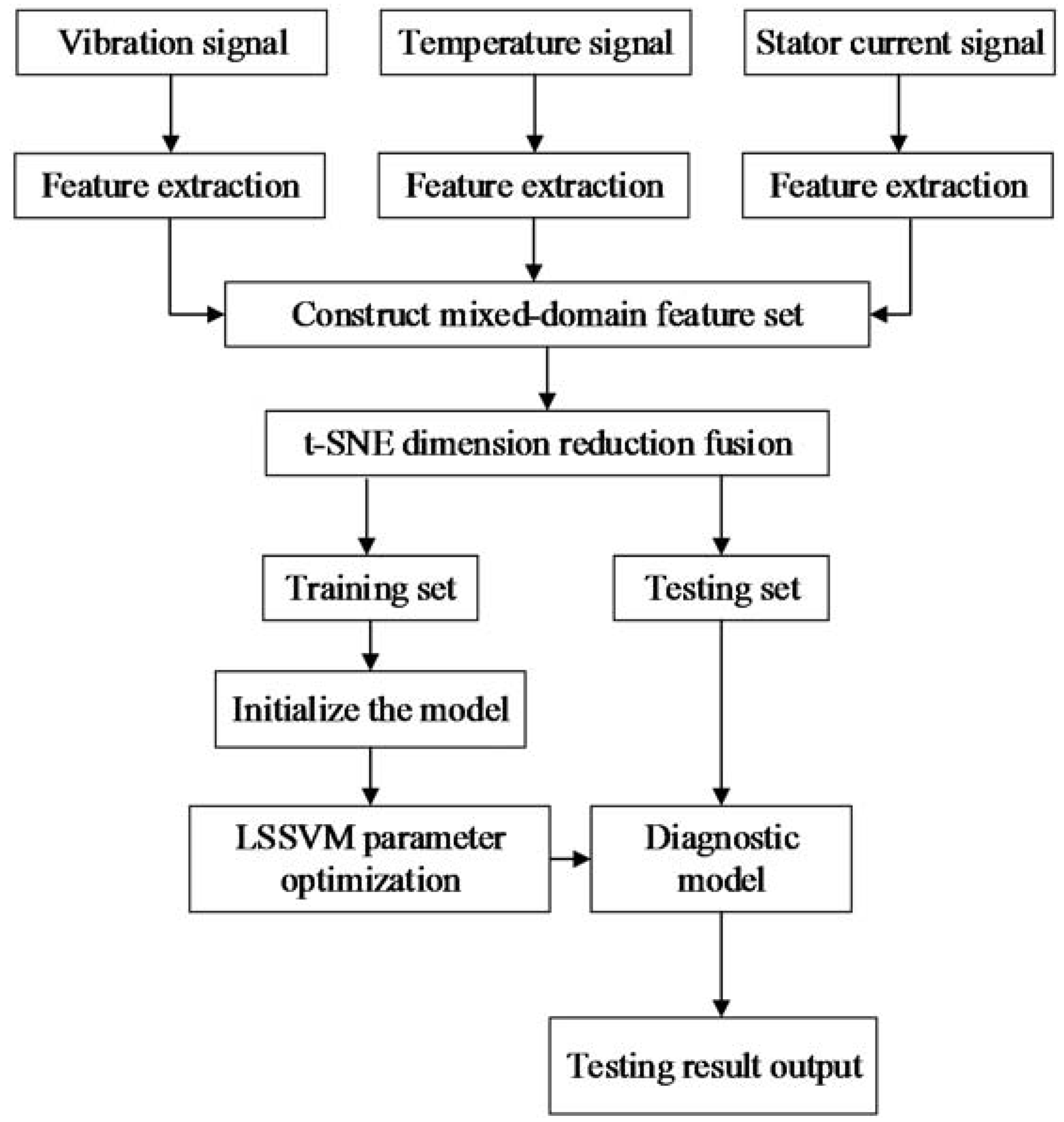
The diagnosis status can be divided into four categories: “0” indicates normal working conditions, “1” indicates parallel misalignment, “2” indicates angle misalignment, and “3” indicates integrated misalignment. According to the data obtained from the simulation, each type had 100 samples (of which 60 samples are for training and 40 samples are for testing). Fifty-two features were extracted. Then they are dimension reduced by t-SNE. The fusion features were then taken as the input of the least squares support vector machine, the diagnosis was performed according to the process shown in Figure 3. The classification accuracy of training set, testing set and the running time are shown in Table 3. In order to illustrate the superiority of the method described in this paper, the results of the same data set using other parameter optimization methods like trial, grid search, PSO (particle swarm optimization), GA (genetic algorithm), and TUNE (cross-validation) are also listed in Table 3. Table 4 shows the parameters used in various methods.
By comparison, the following conclusions can be drawn:
(1) It takes a slightly shorter time when LSSVM is optimized by TUNE, trial, and Grid Search compared with that by ABC, but the training and testing set classification accuracy of them are not as high as that by ABC. The time is longer when LSSVM is optimized by PSO and GA compared with that by ABC, and the training and testing set both have lower classification accuracy than that by ABC.
(2) It takes slightly shorter time when using trial, Grid Search, TUNE, PSO, and GA to optimize SVM compared with that using ABC. But their classification accuracy of testing set are all lower than that by ABC, though only the training accuracy of SVM_GA is a little higher.
(3) LSSVM optimized by ABC takes about the same amount of time compared with SVM optimized by ABC, but the classification accuracy of training and testing set of LSSVM optimized by ABC is higher.
(4) The training and testing set classification accuracy of LSSVM_ABC is also higher than that of BP. Its classification accuracy is the best.
In order to illustrate the superiority of the model presented in this paper, different signal features with the same dimensionality reduction method were used for the same data set. The operating time, training and testing set accuracy are shown in Table 5.
From Table 5, it can be seen:
(1) The classification accuracy of the three kinds of signals is higher than that of others.
(2) The classification accuracy of any two kinds of signals is higher than that of a single signal.
Therefore, fault diagnosis using heterogeneous information fusion can often achieve better diagnostic results than that of the same kind information.
5. Conclusions
This paper presents a method for fault diagnosis of a wind turbine transmission system based on heterogeneous information fusion. The method uses the collected vibration signal, temperature signal, and stator current signal as original sources, and extracts their time domain, frequency domain, and time-frequency domain as feature values. The t-SNE is used to eliminate the correlation between the 52 feature indexes. The fusion features are then put into the LSSVM, which was optimized by the artificial bee colony algorithm. Simulation tests show that the artificial bee colony optimization model has higher classification accuracy than other optimization models. In the future study, the decision level fusion of heterogeneous information will be deeply integrated to improve the accuracy of fault diagnosis further.
Author Contributions
Y.X. and Y.W. contributed to paper writing and the whole revision process. Z.D. contributed to paper amending. All the authors have read and approved the final manuscript.
Funding
This research was funded by National Natural Science Foundation of China (51577008) and China Scholarship Council (201707095072).
Acknowledgments
The authors are grateful to the anonymous reviewers for their constructive comments on the previous version of the paper.
Conflicts of Interest
The authors declare no conflict of interest.
References
- National Energy Administration. 12th Five-Year Plan of Energy Development; National Energy Administration: Beijing, China, 2013.
- Wind Energy Professional Committee of China Renewable Energy Society. 2016 China Wind Power Capacity Statistics; Wind Energy Professional Committee of China Renewable Energy Society: Beijing, China, 2017. [Google Scholar]
- Global Wind Energy Council. Global Wind Market Development Report 2012. Wind Energy 2013, 4, 32–36. [Google Scholar]
- Zhang, S.; Zhao, Q.; Guo, Y. The Status, Trends and Opportunities of Megawatt Wind Power Generation Technology. Aviat. Power Technol. 2008, 29, 9–13. [Google Scholar]
- Jackon, C. Successful shaft hot-alignment. Hydrocarb. Process. 1999, 6, 28–40. [Google Scholar]
- Shen, D. Fault diagnosis of misalignment of large-scale units. Facil. Manag. Maint. 2010, 5, 52–53. [Google Scholar]
- Sun, Z. Research on Equipment Monitoring and Fault Diagnosis Methods Based on Oil Analysis Technology; Taiyuan University of Technology: Taiyuan, China, 2012. [Google Scholar]
- Cao, L.; Li, A.; Deng, Y.; Ding, Y. Application of acoustic emission and wavelet packet analysis in damage condition monitoring. Vib. Test Diagn. 2012, 32, 591–595. [Google Scholar]
- Xu, Z. Research on Condition Monitoring and Fault Diagnosis of Wind Turbine Drive Train Based on Vibration Method; Zhejiang University: Hangzhou, China, 2012. [Google Scholar]
- Hou, J. Research on Fault Diagnosis Method of Rotor Bearing System Based on Motor Current; Taiyuan University of Technology: Taiyuan, China, 2015. [Google Scholar]
- Shen, C. Research on Fault Diagnosis and Prediction of Key Components of Rotating Machinery and Equipment; University of Science and Technology of China: Hefei, China, 2014. [Google Scholar]
- Long, J.; Wu, J. Rotor Misalignment of Wind Turbine Generator. Noise Vib. Control 2013, 3, 222–225. [Google Scholar]
- Zhang, T. Fault Diagnosis of Gear Transmission Based on Bispectrum Analysis of Motor Current Signal. J. Mech. Eng. 2012, 21, 84–90. [Google Scholar] [CrossRef]
- Hou, J.; Ding, H.; Yang, Z. Fault Diagnosis of Rotor Bearing System Based on Stator Current. Coal Technol. 2015, 34, 268–271. [Google Scholar]
- Zhang, X.; Ruan, S.; Zhou, X.; Zhao, H. Prediction method for early failure of main bearing of wind turbine based on condition monitoring. Guangdong Electr. Power 2012, 11, 7–50. [Google Scholar]
- Fang, R.; Jiang, S.; Shang, R.; Wang, L. On-line evaluation cloud model of wind turbine gearbox using trend state analysis. J. Huaqiao Univ. 2016, 37, 32–37. [Google Scholar]
- Li, H.; Li, X.; Hu, Y.; Yang, C.; Zhao, B. Unequally spaced grey prediction of operating parameters of wind turbines. Autom. Electr. Power Syst. 2012, 9, 29–33. [Google Scholar]
- An, B.; Zhai, Y.; Zhao, J.; Li, H.; Hou, Y. Fault diagnosis of wind turbine gearbox based on KPCA-RVM. Comput. Eng. Appl. 2017, 53, 207–211. [Google Scholar]
- Zhen, L. Gearbox Fault Diagnosis Based on Feature Fusion of Different Information; North China Electric Power University: Beijing, China, 2014. [Google Scholar]
- Hong, Y. Fault Diagnosis of Misalignment for Transmission System of Doubly-Fed Wind Turbines Based on Stator Current; Beijing Jiaotong University: Beijing, China, 2018. [Google Scholar]
- Kang, N. Research on Misalignment Fault Diagnosis of Double-Fed Wind Turbine Transmission System; Beijing Jiaotong University: Beijing, China, 2017. [Google Scholar]
- Guo, P.; Infield, D.; Yang, X. Monitoring and analysis of temperature trend of wind turbine gearbox. Proc. CSEE 2011, 31, 129–136. [Google Scholar]
- Fu, Q. Research on Rotor Vibration Fault Diagnosis Method Based on Information Fusion; Shenyang Aerospace University: Shenyang, China, 2012. [Google Scholar]
- Jin, J.; Wu, F. Development and Prospect of Information Fusion Technology. Comput. Dev. Appl. 2006, 19, 50–53. [Google Scholar]
- Liang, J.; Yang, W.; Cai, X. Fuzzy Integration Method for Decision Fusion. J. Xidian Univ. 1998, 29, 86–90. [Google Scholar]
- Li, L. Research on Rotor Dual-Section Information Fusion and Fault Diagnosis; Zhengzhou University: Zhengzhou, China, 2009. [Google Scholar]
- Shao, R.; Hu, W.; Wang, Y.; Qi, X. The fault feature extraction and classification of gear using principal component analysis and kernel principal component analysis based on the wavelet packet transform. Measurement 2014, 54, 118–132. [Google Scholar] [CrossRef]
- Wang, G.; Zhang, P.; Li, B.; Liu, C.; Zhang, A. Feature extraction method based on morphological spectrum of abrasive grain image. Lubr. Seal. 2011, 36, 30–32. [Google Scholar]
- Liu, H.; Yang, J.; Wang, Y. Research on acoustic target feature extraction method based on manifold learning. Acta Phys. Sin. 2011, 60, 444–450. [Google Scholar]
- Li, F.; Tang, B.; Dong, S. Fault diagnosis model based on feature reduction with orthogonal neighborhood retention. Chin. J. Sci. Instrum. 2011, 3, 621–627. [Google Scholar]
- Xia, L.; Hu, N.; Qin, G. Turbine Pump Mass Data Anomaly Recognition Algorithm Based on Manifold Learning. J. Aerosp. Power 2011, 26, 698–703. [Google Scholar]
- Gu, Y. Research on Early Fault Diagnosis Technology and System of Large Wind Turbine Gearbox; Institute of Machinery Science: Beijing, China, 2016. [Google Scholar]
- Li, Y.; Zhang, Y.; Xu, Y.; Wang, J.; Miao, Z. Image Data Set Visualization Method Based on Depth Features and Nonlinear Dimension Reduction. Appl. Res. Comput. 2017, 34, 621–625. [Google Scholar]
- Fei, C.; Ai, Y.; Wang, L.; Li, C. Research on Vibration Fault Diagnosis Technology of Aeroengine Based on Support Vector Machine. J. Shenyang Univ. Aeronaut. Astronaut. 2010, 27, 29–32. [Google Scholar]
- He, X.; Zhao, H. Support vector machine and its application in mechanical fault diagnosis. Cent. South Univ. 2005, 36, 97–101. [Google Scholar]
- Jia, R.; Xu, Q.; Li, H.; Liu, W.; Yang, K. Transformer fault diagnosis using least squares support vector machine multi-classification method. High Volt. Technol. 2007, 33, 110–132. [Google Scholar]
- Zhang, J.; Yan, Y.; Wang, S. Fault Diagnosis of Fan Gearbox Based on Wavelet Decomposition and Least Squares Support Vector Machine. Trans. Microsyst. Technol. 2011, 30, 41–43. [Google Scholar]
- Guo, H.; Liu, H.; Wang, L. Least Squares Support Vector Machine parameter selection method and its application. J. Syst. Simul. 2006, 18, 2033–2036. [Google Scholar]
- Zhao, J. Research and Application of Swarm Intelligence Algorithm; Jiangnan University: Wuxi, China, 2010. [Google Scholar]
- Karaboga, D.; Akay, B. A Comparative Study of Artificial Bee Colony Algorithm. Appl. Math. Comput. 2009, 214, 108–132. [Google Scholar] [CrossRef]
- Yu, M.; Ai, Y. Optimization and Application of Support Vector Machine Parameters Based on Artificial Bee Colony Algorithm. Optoelectron.·Laser 2012, 23, 374–378. [Google Scholar]
- Karaboga, D. An Idea Based on HoneyBee Swarm for Numerical Optimization; Technical Report-TR06; Erciyes University: Kayseri, Turkey, 2005. [Google Scholar]
- Wang, D. Analysis and Diagnosis Technique of Misalignment Failure. Equip. Manag. Maint. 2005, 10, 29–31. [Google Scholar]
- Long, J.; Wu, J. Fault Diagnosis of Rotor Misalignment for Windmill Generators. Noise Vib. Control 2013, 33, 222–225. [Google Scholar]
- Liu, R.; Hu, S. Simulation of Misalignment of Gear Coupling Based on Virtual Prototype. Fan Technol. 2009, 2, 49–52. [Google Scholar]
- Xiao, Y.; Kang, N.; Hong, Y.; Zhang, G. Misalignment Fault Diagnosis of DFWT Based on IEMD Energy Entropy and PSO-SVM. Entropy 2017, 19, 6. [Google Scholar] [CrossRef]
- Xiao, Y.; Hong, Y.; Chen, X.; Chen, W. The Application of Dual-Tree Complex Wavelet Transform (DTCWT) Energy Entropy in Misalignment Fault Diagnosis of Doubly-Fed Wind Turbine (DFWT). Entropy 2017, 19, 587. [Google Scholar] [CrossRef]
- Zhang, G. Thermal Characteristics Analysis of High Speed Transmission System of Wind Turbines; Beijing Jiaotong University: Beijing, China, 2017. [Google Scholar]
- Kang, Y.; Wang, C.C.; Chang, Y.P. Gear Fault Diagnosis in Time Domains by Using Bayesian Networks. Adv. Soft Comput. 2007, 37, 741–751. [Google Scholar]
- Wu, S.; Liu, C.; Gao, L. Research on Fault Sensitivity Experiment of Frequency Domain Feature. Mach. Tools Hydraul. 2012, 40, 169–172. [Google Scholar]
Figure 1.
Three kinds of fusion structure. (a) Data Level Fusion; (b) Feature Level Fusion; (c) Decision Level Fusion.
Figure 1.
Three kinds of fusion structure. (a) Data Level Fusion; (b) Feature Level Fusion; (c) Decision Level Fusion.

Figure 2.
Principle of the artificial bee colony algorithm.
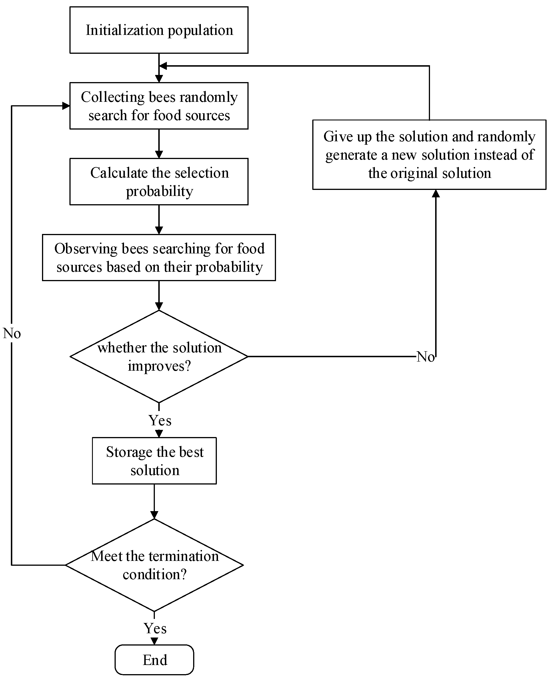
Figure 3.
The fault diagnosis process.

Table 1.
Mixed feature library of vibration signals.
| Feature Library | Feature | Index |
|---|---|---|
| Mixed-domain feature library | Time Domain | root mean square, square root amplitude, variance, standard deviation, kurtosis, waveform index, peak index, pulse index, margin index, kurtosis index |
| Frequency domain | center of gravity frequency, mean square frequency, frequency variance | |
| Time-frequency domain | the first eight energy entropy of the IMF (intrinsic mode function) component of IEMD decomposition |
Table 2.
Mixed feature library of stator current signals.
| Feature Library | Feature | Index |
|---|---|---|
| Mixed-domain feature library | Time Domain | root mean square, square root amplitude, variance, standard deviation, kurtosis, waveform index, peak index, pulse index ,margin index, kurtosis index |
| Frequency domain | center of gravity frequency, mean square frequency, root mean square frequency, frequency variance | |
| Time-frequency domain | sample entropy 1–5, energy entropy H1, H2, H3, H4, H5, spectral kurtosis a1, a2, a3, a4, a5 |
Table 3.
Results of different fault diagnosis methods.
| Method | Running Time (s) | Training Set Classification Accuracy | Testing Set Classification Accuracy |
|---|---|---|---|
| LSSVM_ABC | 42.9409 | 100% (240/240) | 96.25% (154/160) |
| LSSVM_trial | 13.2171 | 97.0833% (233/240) | 93.125% (149/160) |
| LSSVM_Grid Search | 39.0374 | 100% (240/240) | 27.5% (44/160) |
| LSSVM_TUNE | 17.4725 | 95.4167% (229/240) | 93.75% (150/160) |
| LSSVM_PSO | 196.5356 | 99.1667% (238/240) | 94.375% (151/160) |
| LSSVM_GA | 66.7908 | 92.5% (222/240) | 91.875% (147/160) |
| SVM_ABC | 44.1836 | 99.1667% (238/240) | 95.625% (153/160) |
| SVM_trial | 7.5427 | 93.3333% (224/240) | 91.875% (147/160) |
| SVM_Grid Search | 38.1483 | 98.3333% (236/240) | 94.375% (151/160) |
| SVM_TUNE | 23.7067 | 98.3333% (236/240) | 93.75% (150/160) |
| SVM_PSO | 43.4475 | 95.8333% (230/240) | 93.75% (150/160) |
| SVM_GA | 40.9686 | 100% (240/240) | 72.5% (116/160) |
| BP (Back Propagation) neural network | 33.1814 | 82.5% (198/240) | 81.875% (131/160) |
Table 4.
Parameters used in various methods.
| Method | C | σ |
|---|---|---|
| LSSVM_ABC | 3.1355 | 4.4392 |
| LSSVM_trial | 10 | 1 |
| LSSVM_Grid Search | 0.7071 | 0.0884 |
| LSSVM_TUNE | 1.0143 | 232.1482 |
| LSSVM_PSO | 58.2596 | 99.6819 |
| LSSVM_GA | 9.1064 | 479.2951 |
| SVM_ABC | 3.14 | 4.4384 |
| SVM_trial | 1 | 0.01 |
| SVM_Grid Search | 1.4142 | 0.0884 |
| SVM_TUNE | 2.639 | 0.0544 |
| SVM_PSO | 5.4266 | 0.01 |
| SVM_GA | 15.8506 | 82.3615 |
The structure of BP is 6-10-4, ‘traingdx’ and ‘learngdm’ algorithms, maximum training step is 500, learning rate is 0.01, and minimum training error is 0.01.
Table 5.
Diagnostic results of different signals.
| Signal Selection | Running Time (s) | Training Set Classification Accuracy | Testing Set Classification Accuracy |
|---|---|---|---|
| Vibration signal | 43.6846 | 100% (240/240) | 85.625% (137/160) |
| Temperature signal | 43.0802 | 90.8333% (218/240) | 81.25% (130/160) |
| Electrical signal | 43.1965 | 99.5833% (239/240) | 84.375% (135/160) |
| Vibration signal + temperature signal | 43.1038 | 100% (240/240) | 93.75% (150/160) |
| Vibration Signal + Electrical Signal | 43.5408 | 100% (240/240) | 88.75% (142/160) |
| Temperature signal + electrical signal | 43.0321 | 100% (240/240) | 95% (152/160) |
| Three signals | 42.9409 | 100% (240/240) | 96.25% (154/160) |
© 2018 by the authors. Licensee MDPI, Basel, Switzerland. This article is an open access article distributed under the terms and conditions of the Creative Commons Attribution (CC BY) license (http://creativecommons.org/licenses/by/4.0/).
Share and Cite
MDPI and ACS Style
Xiao, Y.; Wang, Y.; Ding, Z. The Application of Heterogeneous Information Fusion in Misalignment Fault Diagnosis of Wind Turbines. Energies 2018, 11, 1655. https://doi.org/10.3390/en11071655
AMA Style
Xiao Y, Wang Y, Ding Z. The Application of Heterogeneous Information Fusion in Misalignment Fault Diagnosis of Wind Turbines. Energies. 2018; 11(7):1655. https://doi.org/10.3390/en11071655
Chicago/Turabian StyleXiao, Yancai, Yujia Wang, and Zhengtao Ding. 2018. "The Application of Heterogeneous Information Fusion in Misalignment Fault Diagnosis of Wind Turbines" Energies 11, no. 7: 1655. https://doi.org/10.3390/en11071655
Note that from the first issue of 2016, this journal uses article numbers instead of page numbers. See further details here.