Short-Term Wind Speed Forecasting Based on Low Redundancy Feature Selection

Abstract

Wind speed forecasting is an indispensable part of wind energy assessment and power system scheduling. In the modeling of wind speed forecasting, there are problems of insufficiency of the high input feature dimension, weak pertinence of the model and a lack of consideration about the redundancy between features. To address these problems, a short-term wind speed forecast method based on low redundancy feature selection is proposed. Firstly, complementary ensemble empirical mode decomposition (CEEMD) is used to pretreat the wind speed data to reduce the randomness and fluctuation of wind speed data. Secondly, conditional mutual information (CMI) is used to analyze the correlation between the input features on different predicted days and wind speed series. The feature order based on conditional mutual information is used to reduce the redundancy between candidate features and establish subsets with candidate features. After that, according to different candidate feature subsets of different predicted days, the outlier-robust extreme learning machine (ORELM) is used to carry out the forward feature selection and obtain optimal feature subsets for different predicted days. Finally, the optimal prediction model is constructed by using the optimal feature subset and the short-term wind speed forecasting is carried out. The validity and advance of the new method are verified by measured data through comparison experiments.

1. Introduction

Wind energy is one of the renewable energy sources that could replace fossil fuels. It has grown rapidly in the past decades. By the end of 2015, the cumulative installed capacity of wind energy around the world reached 43.29 GW [1,2]. Large-scale wind energy integration into power grid has brought operational problems because of the randomness and volatility of wind power generation [3,4]. High precision wind power prediction is one of the solutions for optimizing the power reserves, which is used to balance the fluctuations of wind power. With the assistance of accurate wind power forecasting, the stability of power system operation and the adopt capacity for wind power could be improved [5,6].

Wind speed forecasting is one of the basic components of wind power forecasting. The wind speed forecasting for the next 30 min to 6 h can be classified as short-term wind speed forecasting [7], which can meet the need of power producer on managing the grid operations, reducing the negative impact of wind power volatility in power grid operation [8]. The existing wind speed forecasting model construction can be generally divided into three steps: data preprocessing, feature selection and optimal model construction.

The collected original wind speed data has strong randomness and volatility, the outlier data contained can influence the training effect of the prediction model. The existing research uses signal processing to preprocess original wind speed data, which can reduce the effect of outlier wind speed data on the prediction model [9]. At present, among the signal processing method applied to wind speed data preprocessing. Empirical Mode Decomposition (EMD) has remarkable self-adaptability and suitable for processing nonlinear data, but it is prone to modal-mixing issues [10]. To solve the problem of modal-mixing, Ensemble Empirical Mode Decomposition (EEMD) introduces white noise signals into the original signals, but the decomposition result is contaminated by noise components [11]. Complementary Ensemble Empirical Mode Decomposition (CEEMD) is an improvement based on EEMD, which can address the defects of noise components by counteracting the noise components in the decomposition result with two groups of noise signals which have opposite phase [12]. Therefore, CEEMD can effectively reduce the randomness and volatility of wind speed data under the premise that the wind speed signal is not contaminated by noise components.

Feature selection is an effective approach to reduce the feature dimensions of wind speed forecasting models that can directly improve the prediction accuracy. By introducing as many meteorological factors as possible, the prediction model can reflect the effect of complex external conditions on wind speed to a certain extent. However, too many input features also greatly complicated the model. High redundancy between input features reduced the prediction accuracy and efficiency of the prediction model. To reduce the prediction complexity, the existing researches choose the optimal feature subset through feature selection process [13]. Among the existing feature selection methods, filter methods use some predefined evaluation criteria to evaluate the importance of features for prediction or classification. On this basis, forward feature selection or backward feature selection is carried out through a special feature order obtained by correlation analyzing methods. Filter methods have the characteristics of fast speed and small calculation, which offers strong advantages in engineering applications [14].

The relevance and redundancy between features can directly affect the result of filter feature selection methods. Among the correlation analyzing methods, Mutual Information (MI) can analyze the correlation between feature subset and prediction target, but the result of MI lacks consideration of the redundancy features inside the feature subset [15]. When analyzing the relevance between a feature and the predicted object, Conditional Mutual Information (CMI) also considered the redundancy between the feature and other selected features, so CMI can maintain low redundancy among the feature subset under the premise of ensuring the feature subset is strongly relevant to the predicted object [16]. With the assistance of the feature order obtained by CMI, filter feature selection can effectively improve the prediction accuracy. Meanwhile, existing studies usually analyze the relationship between wind speed and related features based on annual historical data, not considering the correlation between wind speed and complex meteorological factors in different periods of a year, which can’t fully meet the needs of the wind speed forecasting in the different periods [17].

The methods of wind speed predictor construction can be divided into physical methods, statistical methods, intelligent methods and hybrid methods [18]. Statistical methods only need historical data to establish the mapping relationship between input features and time series of wind speed, and then carry out the prediction through this mapping relationship [19]. Representative statistical methods include the Kalman filter [20] and autoregressive moving average (ARMA) methods [21]. The intelligent methods can dig into the potential relationship between the input feature and the time series of wind speed through historical data, which is more suitable to deal with complicated relationships than the traditional statistical methods [22]. The intelligent methods include artificial neural networks [23] and Recurrent Neural Networks (RNNs) [24]. The artificial neural network methods [23,24,25] have advantage in constructing nonlinear prediction models, which have excellent generalization performance and are suitable for very short-term and short-term wind speed forecasting [26].

Among the artificial neural network methods, Extreme Learning Machine (ELM) has the advantages of extremely fast learning speed and generalization performance compared with traditional neural network, but it easily runs into partial optimization problems [27]. Outlier-Robust Extreme Learning Machine (ORELM) improves the ELM generalization ability by introducing standard parameters, and is more suitable for forecasting wind speeds which have characteristics of high randomness [28].

According to the deficiency of existing methods, a multi-step prediction method based on low redundancy feature selection is proposed. Firstly, the CEEMD method was used to pretreat the training set wind speed data. Then, a low redundancy forward feature selection was conducted based on ORELM and the order of feature importance gained by CMI. Finally, the optimal short-term wind speed forecasting model is constructed with the optimal feature subset to predict the specific period wind speed. The feasibility and effectiveness of the new method are proved through the measurement data of the American wind energy technology center.

2. Structure and Methodology of the New Hybrid Model

The data of training set was pretreated by CEEMD to reduce the effect of outlier data on prediction model. CMI is used to reduce the redundancy of feature selection results. Construct ORELM predictor with low redundancy optimal feature subset to improve the generalization ability of the predictor.

2.1. Complementary Ensemble Empirical Mode Decomposition (CEEMD)

CEEMD is an improved method on the basis of EMD and EEMD, the specific iteration of EMD is generated as follows [29]:

(a)

The local maximum and minimum points of the original signal $S$ are connected by a cubic spline to obtain the upper envelope $e_{\max }$ and the lower envelope $e_{\min }$.

(b)

The sequence $m_1=[e_{\max }+e_{\min }]/2$ is obtained by averaging two envelopes.

(c)

The first component h₁ is obtained by removing m₁ from S:

$$h_1=S-m_1$$

(1)

(d)

Repeat the above steps with h₁ until the number of extrema and zero crossings is equal or differ at most by one, and the mean value of $e_{\max }$ and $e_{\min }$ is zero. The remaining signal is the first Intrinsic Mode Functions (IMF).

(e)

Remove IMF₁ from the original S and repeat the iterations above until the signal cannot be decomposed, the remaining signal is the remainder function.

With the assistance of noise signals, EEMD makes up for the defects of EMD’s prone to model-mixing by using the characteristics of the uniform distribution of the noise spectrum [11]. However, the residue noise during the signal reconstruction is difficult to be tolerated, which affects the efficiency of EEMD decomposition. The fallowing improvement has been carried out based on EEMD:

(a)

Two groups of white noise signals with the same amplitude $N$ and opposite phase are introduced into the original signal $S$ respectively, get two generated signals $M_1=S+N$ and $M_2=S-N$;

(b)

Decomposition two groups of sequences with EMD method, obtain two groups of IMFs $im{f}_{x1}$ and $im{f}_{x2}$. Then obtain the IMFs of CEEMD by averaging the components of the two groups of IMFs:

$$imf=(im{f}_{x1}+im{f}_{x2})/2$$

(2)

(c)

Repeat the above steps with the data which removed the IMFs until the signal cannot be decomposed. The remainder function $r_n(t)$ is the remainder of the signal, and the final decomposition result of CEEMD is:

$$x(t)={\displaystyle \sum _{i=1}^{n}im{f}_i(t)}+r_n(t)$$

(3)

CEEMD solves the defect of EMD being prone to mode-mixing, and eliminates the effect of white noise induced by EEMD by frequency domain complementation [30].

2.2. Conditional Mutual Information (CMI)

The CMI method can calculate the correlation between the target feature and the predicted target with condition of the lowest redundancy between the target feature and the selected features. The MI method uses the probability density function to define the correlation between variables X and Y, the formula is as follows [31]:

$$I(X;Y)={\displaystyle \sum _{y\in Y}{\displaystyle \sum _{x\in X}\mathrm{P}(x,y)\log \left(\frac{\mathrm{P}(x,y)}{\mathrm{P}(x)\mathrm{P}(y)}\right)}}$$

(4)

where $\mathrm{P}(x)$ and $\mathrm{P}(y)$ represent the marginal probability distribution functions of sample X and Y respectively. $\mathrm{P}(x,y)$ represents the joint probability density function for sample x and sample y. The larger the MI value of the feature is, the higher the correlation between it and the predicted target [16].

In the condition of a given discrete random variable Z, the CMI between X and Y can be expressed as $I\left(X;Y|Z\right)$. In the process of wind speed forecasting, assuming that the original feature set is V, the given condition is the selected feature set $V_j$, CMI between the target variable C and the selected feature $V_i$ is:

$$I(C;V_i|V_j)=I(C;V_i)-I(C;V_i;V_j)$$

(5)

where $I(C;V_i)$ represents MI between the target variable C and the selected feature $V_i$ (the correlation between features), $I(C;V_i;V_j)$ represents that the information overlaps between feature $V_i$ and feature $V_j$ meanwhile as the target variable (the redundancy between features).

In conclusion, based on the MI between features and target variables, the CMI method reduces the redundancy between features as another indicator of feature evaluation. It has not only evaluated the contribution of features to the accuracy of prediction model, but also ensured the low redundancy of the corresponding feature arrangement modes. Therefore, CMI can reduce the effect of redundant information between features on feature selection results.

2.3. Outlier-Robust Extreme Learning Machine (ORELM)

ELM performs the prediction by minimizing the training error, but it is prone to reduce the generalization performance of the model. ORELM introduces specification parameters C to improve ELM generalization ability. ORELM uses ${\ell }_1-\mathrm{norm}$ to replace ${\ell }_2-\mathrm{norm}$, and converts the target function from:

$$\min {\Vert y-H\mathsf{\beta }\Vert }_2^2$$

(6)

to:

$$\underset{\beta }{\min }{\Vert e\Vert }_1+\frac{1}{C}{\Vert \mathsf{\beta }\Vert }_2^2$$

(7)

where $e=y-HB$, $y$ represents the output matrix, $\mathsf{\beta }$ represents the weight matrix between the hidden layer and the output layer. $H$ represents the hidden layer output matrix.

When establishing wind speed forecasting model, assuming a data set with N training samples $(x_i,y_i),i\in [1,N]$, where $x_i$ represents the input matrix, $y_i$ represents the output matrix. Assume that $g(x)$ represents the activation function, and the number of hidden layer nodes is L. The iterations of the ORELM algorithm are as follows:

(a)

The implicit layer node parameters, namely the weight matrix $w_i$ and the threshold $b_i$ are randomly generated, where $i\in [1,L]$;

(b)

Calculate the output matrix of the hidden layer [32]:

$$\begin{array}{l}H(w_1,\dots ,w_L,x_1,\dots ,x_N,b_1,\dots ,b_L),\\ =\left[\begin{array}{l}g(w_1\cdot x_1+b_1)\cdots g(w_L\cdot x_1+b_L)\\ ⋮⋮\\ g(w_1\cdot x_N+b_1)\cdots g(w_L\cdot x_N+b_L)\end{array}\right]\end{array}$$

(8)

(c)

Parameter initialization: $\mu =2N/{\Vert y\Vert }_1$, where $\mu$ represents penalty coefficient, $e_1=0$, the Lagrange multiplier ${\lambda }_1=0$;

(d)

This constraint optimization problem is solved by using the augmented Lagrange multiplier (ALM) method, execute the following iteration process until the loop parameter k reaches the maximum number of iterations:

$$\{\begin{array}{l}{\mathsf{\beta }}_{k+1}={(H^{T}H+2/C\mu I)}^{-1}{H}^T(y-e_k+{\lambda }_k/\mu )\\ e_{k+1}=shrink(y-H{\mathsf{\beta }}_{k+1}+{\lambda }_k/\mu ,1/\mu )\\ {\lambda }_{k+1}={\lambda }_k+\mu (y-H{\mathsf{\beta }}_{k+1}-e_{k+1})\end{array}$$

(9)

ORELM avoided solving the sparse matrix by converting the ELM’s target function into a manageable convex relaxation problem. In addition, the ALM method is adopted to deal with the convex relaxation problem, and the ability of prediction model to deal with discrete data is strengthened, the generalization performance of ELM is improved [28].

2.4. Forecasting Accuracy Evaluations

For performance evaluation model, using Root-Mean-Square Error (RMSE) and Mean Absolute Percentage Error (MAPE) as the index to evaluate model performance, which are widely used in the wind speed forecasting field. The RMSE and MAPE are calculated as follows:

$$\mathrm{RMSE}=\sqrt{\frac{1}{T}{\displaystyle \sum _{t=1}^T(x_t-{\widehat{x}}_t{)}^2}}$$

(10)

$$\mathrm{MAPE}=\frac{1}{T}{\displaystyle \sum _{t=1}^T\left|\frac{x_t-{\widehat{x}}_t}{x_t}\right|}\times 100\%$$

(11)

where ${\widehat{x}}_t$ represents the predicted value corresponding to the real wind speed $x_t$, T represents the number of wind speed samples.

3. The Composition of Data Sets

3.1. The Features of The Input Set

The wind speed at different time periods of a year has different characteristics and is affected by the surface roughness and air density. Wind shear (1/s) can reflect the surface roughness around the wind tower and the rate of wind velocity at different heights [33]. Temperature (°C), pressure (mBar) and humidity are variables that able to influence the air density and can affect wind speed [34]. Therefore, when building the original feature set, the basic features include wind speed x_t (m/s), temperature T_t (°C), relative humidity R_t (%), absolute humidity S_t (g/Kg), atmospheric pressure P_t (mBar) and wind shear C_t (1/s) of the 16 historical time points (15 min of sampling interval), including the prediction time point t. Meanwhile, the extreme values (max, min), mean, Standard Deviation (std) and Variance (var) of each feature were counted as supplementary features, the final feature dimension is 126. The original historical features and their feature numbers are shown in

Table 1. The original historical feature set and the features’ serial number.

Feature Types	Historical Features	Numbers
Wind speed (xt)	xt−1,xt−2,xt−3,…,xt−16	1–16
Temperature (Tt)	Tt−1,Tt−2,Tt−3,…,Tt−16	17–32
Relative humidity (Rt)	Rt−1,Rt−2,Rt−3,…,Rt−16	33–48
Absolute humidity (St)	St−1,St−2,St−3,…,St−16	49–64
atmospheric pressure (Pt)	Pt−1,Pt−2,Pt−3,…,Pt−16	65–80
Wind shear (Ct)	Ct−1,Ct−2,Ct−3,…,Ct−16	81–96

. The original statistical features and their feature numbers are shown in

Table 2. The original statistical feature set and the features’ serial number.

Feature Types	Statistical Features	Numbers
Wind speed (xt)	max(xt−1, xt−2, xt−3,…, xt−16); min(xt−1, xt−2, xt−3,…, xt−16); mean(xt−1, xt−2, xt−3,…, xt−16); std(xt−1, xt−2, xt−3,…, xt−16); var(xt−1, xt−2, xt−3,…, xt−16)	97–101
Temperature (Tt)	max(Tt−1, Tt−2, Tt−3,…, Tt−16); min(Tt−1, Tt−2, Tt−3,…, Tt−16); mean(Tt−1, Tt−2, Tt−3,…, Tt−16); std(Tt−1, Tt−2, Tt−3,…, Tt−16); var(Tt−1, Tt−2, Tt−3,…, Tt−16)	102–106
Relative humidity (Rt)	max(Rt−1, Rt−2, Rt−3,…, Rt−16); min(Rt−1, Rt−2, Rt−3,…, Rt−16); mean(Rt−1, Rt−2, Rt−3,…, Rt−16); std(Rt−1, Rt−2, Rt−3,…, Rt−16); var(Rt−1, Rt−2, Rt−3,…, Rt−16)	107–111
Absolute humidity (St)	max(St−1, St−2, St−3,…, St−16); min(St−1, St−2, St−3,…, St−16); mean(St−1, St−2, St−3,…, St−16); std(St−1, St−2, St−3,…, St−16); var(St−1, St−2, St−3,…, St−16)	112–116
atmospheric pressure (Pt)	max(Pt−1, Pt−2, Pt−3,…, Pt−16); min(Pt−1, Pt−2, Pt−3,…, Pt−16); mean(Pt−1, Pt−2, Pt−3,…, Pt−16); std(Pt−1, Pt−2, Pt−3,…, Pt−16); var(Pt−1, Pt−2, Pt−3,…, Pt−16)	117–121
Wind shear (Ct)	max(Ct−1, Ct−2, Ct−3,…, Ct−16); min(Ct−1, Ct−2, Ct−3,…, Ct−16); mean(Ct−1, Ct−2, Ct−3,…, Ct−16); std(Ct−1, Ct−2, Ct−3,…, Ct−16); var(Ct−1, Ct−2, Ct−3,…, Ct−16)	122–126

.

Data were collected using measured data from the National Wind Energy Technology Center (NWTC) M2 wind tower. The geographical location of NWTC and M2 wind tower is shown in Figure 1 [35]. The region is located in north latitude 39.91° and west longitude 105.29°, the measured height of the wind speed and temperature is 80 m. The test environment is a personal computer with 16 GB of memory and the Intel(R) Core(TM) i7-6820hk processor which has an operating frequency of 2.7 GHz. The experimental platform is Matlab (R2016a, MathWorks, Natick, MA, USA). The multi-input and multi-output Strategy (MIMO) is more accurate than the rolling prediction method [7]. Therefore, the new method adopts the MIMO prediction structure, which is constructed with the optimal feature subset obtained by low-redundancy forward feature selection, and builds a four-step wind speed forecasting model that meets the requirements of wind speed forecasting in different time periods (the step length is 15 min).

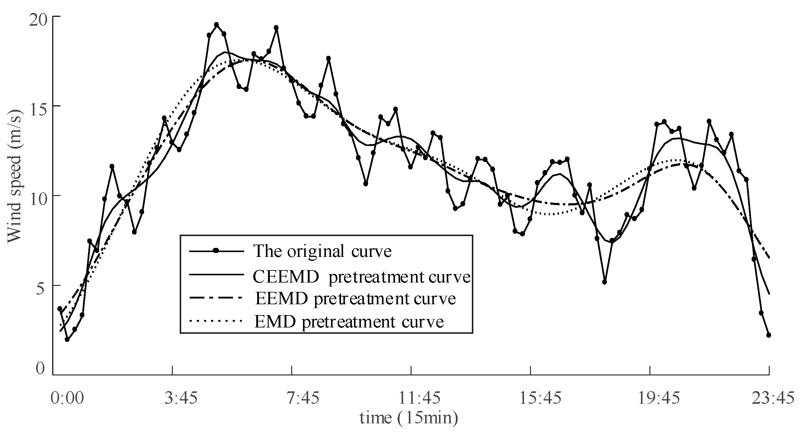
3.2. Data Preprocessing

CEEMD is used to pretreat the signals of wind speed time series. The signal is decomposed into a series of IMFs: ${\mathrm{IMF}}_1,\dots ,{\mathrm{IMF}}_n$. CEEMD parameters are determined by reference to existing literature and statistical experimental conclusions [7], adding a 5 db signal-to-noise ratio white noise to the original signal and the number of iteration is 500. If the high-frequency IMF of wind speed signal fluctuates repeatedly in a very short time, it is indicated that the mode contains more non-cyclical components. Although the volatile component contains a small amount of wind speed information, the large number of outliers in the mode can greatly affect the accuracy and stability of the prediction model. Therefore, CEEMD was used to decompose the wind speed samples to 8 to 10 IMFs, and filter out the highly volatile IMFs, the remaining IMFs reconstructs the new wind speed time series. Thus, the effect of outliers on prediction model is reduced, and the prediction accuracy of model is improved.

To compare the pretreatment impact of CEEMD, EEMD and EMD, the wind speed time series of 31 March 2009 is taken as an example. Figure 2 shows the pretreatment results of three decomposition methods. As shown in Figure 2, the wind speed curve obtained after CEEMD pretreatment reduces the volatility of wind speed, and is more accurately follow the trend of wind speed than other methods in the period from 15:45 to 23:45. Wind speed series after EMD and EEMD pretreatment is difficult to reflect the detailed trend of wind speed.

Meanwhile, in order to test the effect of pretreatment to wind speed forecasting accuracy, a wind speed forecasting experiment is carried out with predictor based on ORELM. The original feature set is used to construct the input feature set. The annual wind speed sample of 2008 is used as the training set, and the data from 30 March to 5 April 2009 is used as the test set.

It can be seen from

Table 3. Result of multistep forecasting for wind speed with data before and after pretreatment.

Pretreatment Method	EMD	EEMD	CEEMD	Raw Data
MAPE	31.96%	29.79%	24.23%	38.16%
RMSE (m/s)	1.5211	1.4013	1.1465	1.9902

that the wind speed sequence obtained after pretreatment with CEEMD is forecasted and got the highest the accuracy. Compared with raw data, RMSE decreased 0.8437 m/s and MAPE decreased 13.93%, which proved that CEEMD effectively reduced the effect of outliers on wind speed forecasting and improves the prediction accuracy.

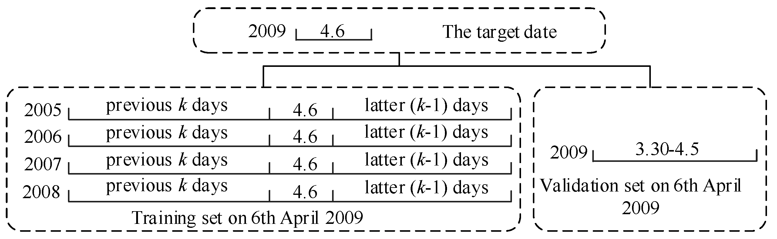
3.3. Data Set Construction

The correlation between wind speed and meteorological factors was different in different time of year. In order to meet the requirements of wind speed forecasting model in different time periods, a method of daily low redundancy wind speed features selection is proposed. Expect the data of the predicted day as target date, the data of k days before and after the target date in the former four years is selected as training set, then analyze the correlation between features with this data set. Meanwhile, data of the week before target date is selected as the validation set, which can ensure feature selection process get feature subsets with strong pertinence based on the meteorological characteristics of different forecast periods. The validation set can also the optimal feature set guaranteed to the meet of target date requirements. Figure 3 shows the data set on 6 April 2009 as an example.

To ensure the new method meets the needs of wind speed forecast at different periods of a year, one day is selected randomly from each quarter of 2009 as the target for prediction (the test set). To test the generalization performance of the new method, new method is used to build the optimal prediction model for every predicted day.

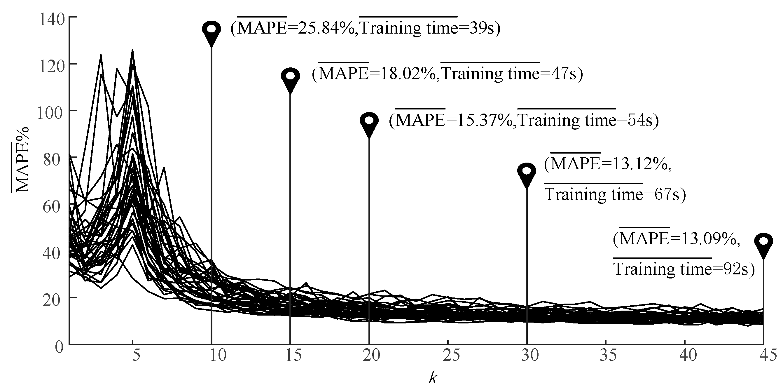
3.4. Data Set Determination

During the training set construction, the parameter of k effects the prediction accuracy and efficiency of models directly. To obtain the appropriate value of parameter k, multi-step prediction models was constructed with different parameters k for 364 days (total 52 weeks) in 2009, and series of statistical experiments was carried out. Figure 4 shows the weekly average error curves with different values of parameter k.

It can be seen from Figure 4 that the training time of models increases with the increase of parameter k, and the MAPE elevation of the parameter k in the interval from 30 to 45 is only 0.03%. In order to ensure the efficiency and accuracy of the new method, the data set with the value of parameter k is set as 30.

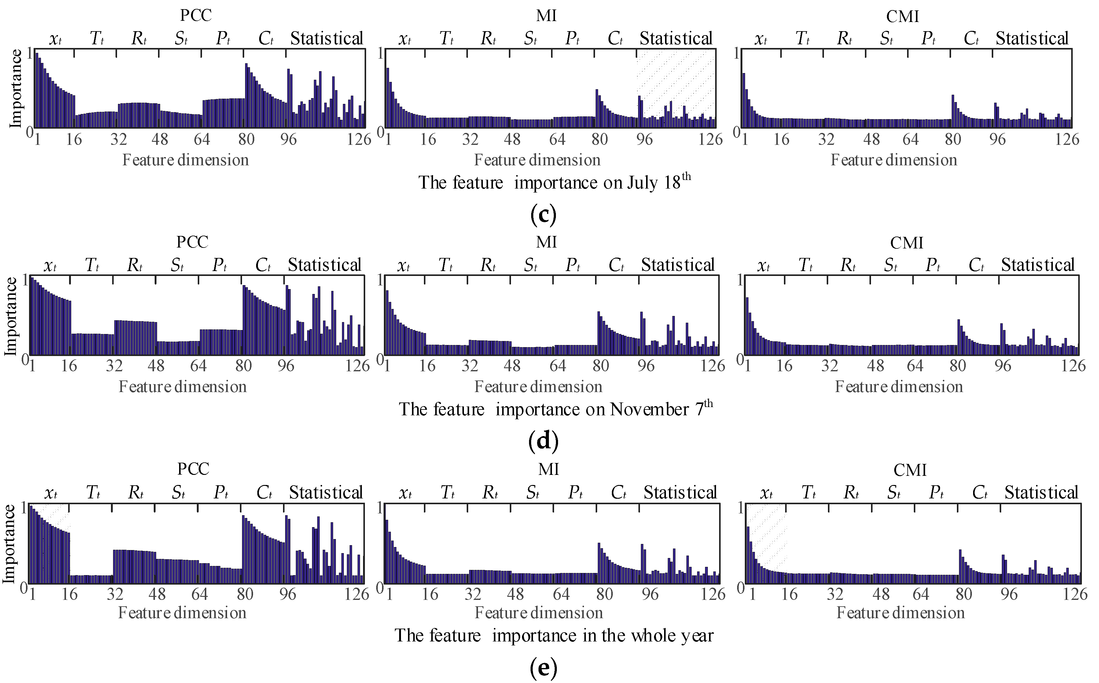
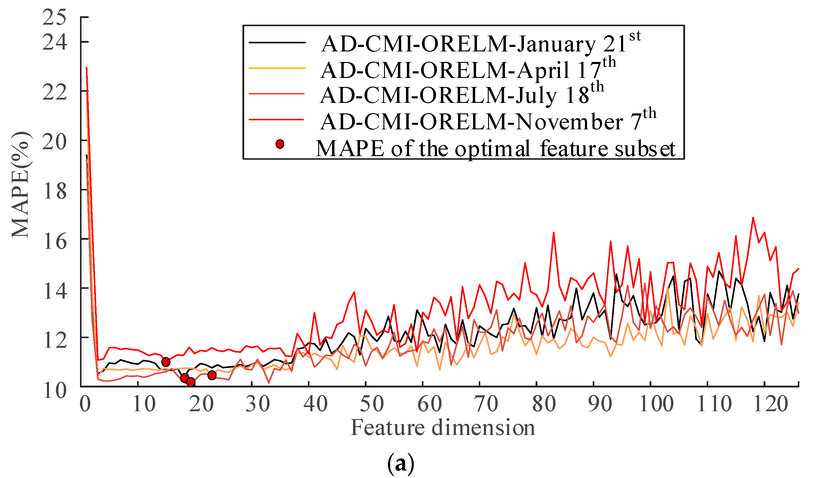
4. Time-Sharing Low Redundancy Feature Selection

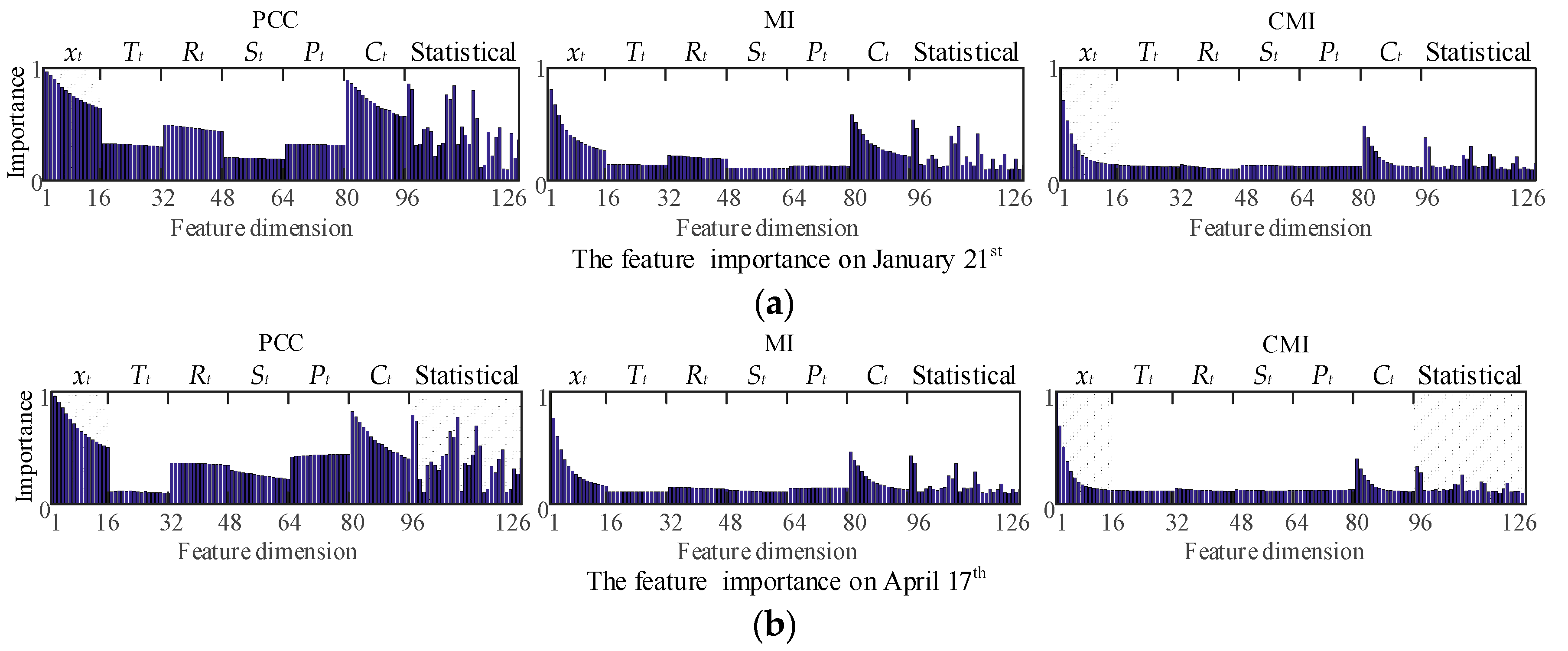
4.1. Analysis of Feature Correlation

To analyze the necessity of the feature selection with historical neighborhood data and the analysis advantage of redundancy feature set gained by CMI, the feature correlation on 21 January, 17 April, 18 July and 7 November 2009 was analyzed according to the Data of Adjacent (AD) and the Data of the whole Year (YD). Figure 5 shows the after the normalization analysis results of Pearson Correlation coefficient [36] (PCC), MI and CMI.

Table 4. Feature numbers of the most important 30 dimensions.

Periods of Time	Analysis Methods	1–10 Dimensional Features	11–20 Dimensional Features	21–30 Dimensional Features
21 January	PCC	1,2,3,4,81,5,82,97,109,6	83,98,114,7,84,8,107,85,9,10	86,108,11,87,12,88,13,14,89,15
	MI	1,2,3,81,4,97,82,5,109,98	83,6,114,84,7,107,8,85,9,10	86,108,11,87,12,13,88,14,15,89
	CMI	1,2,3,81,4,82,97,5,83,109	98,6,84,114,107,7,121,115,85,8	108,9,86,10,11,87,12,88,13,126
17 April	PCC	1,2,3,4,81,5,97,82,109,6	98,83,7,114,84,8,85,9,107,10	86,108,11,12,87,13,88,14,89,15
	MI	1,2,3,4,81,97,5,82,98,109	83,6,7,84,114,8,107,85,9,108	10,86,11,87,12,88,13,121,115,14
	CMI	1,2,3,81,4,97,82,5,98,109	83,6,84,114,7,115,121,107,85,108	8,9,86,10,87,11,33,34,126,120
18 July	PCC	1,2,3,4,81,82,5,97,109,83	6,98,114,84,7,107,85,8,9,86	108,10,87,11,115,12,88,13,89,14
	MI	1,2,3,81,4,82,97,5,98,109	83,6,84,114,107,7,85,8,86,9	108,10,87,11,121,115,88,12,13,89
	CMI	1,2,3,81,4,82,97,5,98,83	109,6,84,107,114,115,121,7,85,108	8,86,9,10,120,126,87,11,122,116
7 November	PCC	1,2,3,4,97,81,5,109,82,6	98,7,83,114,8,84,9,107,10,85	11,12,86,108,13,14,87,15,16,88
	MI	1,2,3,4,81,97,5,109,82,98	6,83,114,7,107,8,84,9,85,10	11,86,12,108,13,14,87,15,16,88
	CMI	1,2,3,81,4,97,82,5,109,98	83,6,114,84,7,107,8,115,121,108	85,9,10,86,11,12,13,14,87,15
YD	PCC	1,2,3,4,5,97,81,109,6,82	98,7,83,8,114,84,9,10,85,11	107,12,108,86,13,14,87,15,16,88
	MI	1,2,3,4,81,97,5,82,109,98	6,83,7,114,84,8,107,9,85,10	11,108,86,12,13,87,14,88,15,16
	CMI	1,2,3,81,4,97,82,5,98,109	83,6,84,7,114,107,121,115,8,85	9,108,86,10,11,87,12,13,88,14

shows numbers of the most important 30-dimensional features.

As can be seen from Figure 5, the importance of the same type of features varies greatly in different dates according to the analysis result with AD dataset. For example, in the analysis results of PCC, feature P_t is higher than the rest periods on 17 April significantly. Table 4 shows that the same correlation analysis method has different importance order for the same feature in different time dates. The analysis results with YD data sets cannot reflect the differences.

Table 4 can be used to compare the redundancy analytical capability between features with different correlation analysis methods. The overlap between features is the redundancy of information, and the redundancy of the same type of features is higher. As can be seen from Table 4, the historical wind speed category features x_t has the highest frequency.

In the first 30 dimensional feature set on 17 April, the PCC method selected 15 dimensions wind speed category features, and the MI method selected the 14 dimensions wind speed category features, while the CMI method only selected the 11 dimensions wind speed category features. Meanwhile, the CMI method took the standard deviation of absolute humidity (115 dimensional) and the variance of air pressure (121 dimensional) into the first 30 dimensional feature set to replenish the information on humidity and air pressure. Similar phenomena occurred in other periods. It can be seen above that CMI method can improve the information integrity of feature subset.

4.2. Forward Feature Selection

The reorder feature gained by PCC, MI and CMI are respectively combined with ORELM, ELM and Back-Propagation Neural Network [25] (BPNN) for forward feature selection. Parameters of ELM and BPNN are set according to relevant references [26,27], the specification parameter C of ORELM is set to 2⁻¹⁰ [28].

To compare the effect of the correlation with AD and YD data sets on predictive models, the feature subset gained with different data sets are combined with the predictors respectively. The forward feature selection is carried out for different forecast days in the condition of different training set and same validation set. MAPE is used to evaluate the prediction accuracy of different method with different feature subset.

Figure 6 shows the error curve of test set in the four predicted days include 21 January, 17 April, 18 July and 7 November 2009, respectively. As shown in Figure 6, the optimal feature subset is determined by the MAPE. Comparing Figure 6a,b, error curves of feature selection with the AD data set converged rapidly and achieved the minimum MAPE, while the error curves of feature selection based on the YD data set converged slowly and the minimum of MAPE is larger.

Table 5. The optimal feature subsets of different predict days obtained with AD data.

Periods of Time	Analysis Methods	AD-ORELM		AD-ELM		AD-BPNN
		MAPE	DIM	MAPE	DIM	MAPE	DIM
21 January	PCC	10.45%	17	11.56%	14	11.39%	103
	MI	10.44%	17	11.33%	21	11.40%	118
	CMI	10.34%	18	11.00%	19	11.03%	116
17 April	PCC	10.75	22	12.19	10	11.93	34
	MI	10.76	23	11.99	18	11.98	90
	CMI	10.37	23	11.56	21	11.87	30
18 July	PCC	10.20	17	11.73	16	11.88	24
	MI	10.23	19	11.82	15	11.97	106
	CMI	10.08	19	11.37	17	11.44	44
7 November	PCC	11.25	15	12.19	15	12.50	88
	MI	11.20	14	12.68	52	12.76	55
	CMI	11.02	15	12.51	15	12.64	59

and

Table 6. The optimal feature subsets of different predict days obtained with YD data.

Periods of Time	Analysis Methods	YD-ORELM		YD-ELM		YD-BPNN
		MAPE	DIM	MAPE	DIM	MAPE	DIM
21 January	PCC	11.11%	106	11.62%	125	11.90%	120
	MI	10.93%	113	11.63%	88	11.83%	121
	CMI	10.71%	83	11.51%	109	11.62%	68
17 April	PCC	11.34%	83	12.77%	53	12.46%	67
	MI	11.23%	97	12.72%	20	12.43%	111
	CMI	11.23%	38	12.32%	56	12.38%	61
18 July	PCC	10.99%	22	12.29%	22	12.34%	21
	MI	10.99%	20	12.22%	21	12.29%	29
	CMI	10.70%	29	12.16%	16	12.24%	27
7 November	PCC	11.52%	81	12.50%	63	12.97%	69
	MI	11.42%	62	12.72%	95	12.90%	57
	CMI	11.37%	94	12.65%	103	12.81%	75

show the prediction effect of predictors based on different optimal feature subsets. As Table 5 and Table 6 show, the optimal MAPE of AD-ORELM decreased by an average of 4.8% compared with YD-ORELM, the optimal MAPE of AD-ORELM decreased by an average of 3.5% compared with YD-ELM, the optimal MAPE of AD-BPNN decreased by an average of 3.7% compared with YD-BPNN, which proved that analyzing feature correlation with AD data can improve the performance of feature selection.

Meanwhile, AD-CMI-ORELM has the highest prediction accuracy in every predicted days, which can be preliminarily proved that the redundancy among the features of the optimal feature subset is reduced by CMI, which improved the prediction accuracy of models.

Table 7. The feature variety of the optimal feature subset obtained by AD-ORELM method.

Periods of Time	Analysis Method	Historical Features		Statistical Features
		xt	Ct	xt	Rt	St	Pt
21 January	PCC	8	4	2	2	1	0
	MI	8	4	2	2	1	0
	CMI	7	4	2	2	2	1
17 April	PCC	10	6	2	3	1	0
	MI	11	6	2	3	1	0
	CMI	9	6	2	3	2	1
18 July	PCC	7	5	2	2	1	0
	MI	9	5	2	2	1	0
	CMI	7	5	2	2	2	1
7 November	PCC	8	3	2	1	1	0
	MI	7	3	2	1	1	0
	CMI	7	4	2	1	1	0

shows types of the optimal features subset obtained by the AD-ORELM method. In combination with Table 5, Table 6 and Table 7, it can be seen that the redundancy of feature subsets can be reduced after appropriate reduction of similar features. This reduction also improved the prediction accuracy. Meanwhile, adding new types of features with high correlation can enhance the information integrity of the feature subset and further reduce MAPE of the optimal feature subset.

The CMI method can control the redundant between features in four predicted days accurately. In the first three predicted days, the feature subsets obtained by CMI introduces the standard deviation of absolute humidity (115 dimensional) and pressure variance (121 dimensional) in the premise of low redundancy, makes the optimal subset of features obtained by CMI is more advantageous than those from MI and PCC in information integrity, and the smaller MAPE is obtained. On 7 November, CMI ensured that the information integrity in the optimal features subset was achieved, resulting in lower MAPE than MI and PCC. In this review, it can be proved that using CMI to carry out low redundancy forward feature selection can effectively improve the prediction accuracy and reduce the dimension of feature subsets.

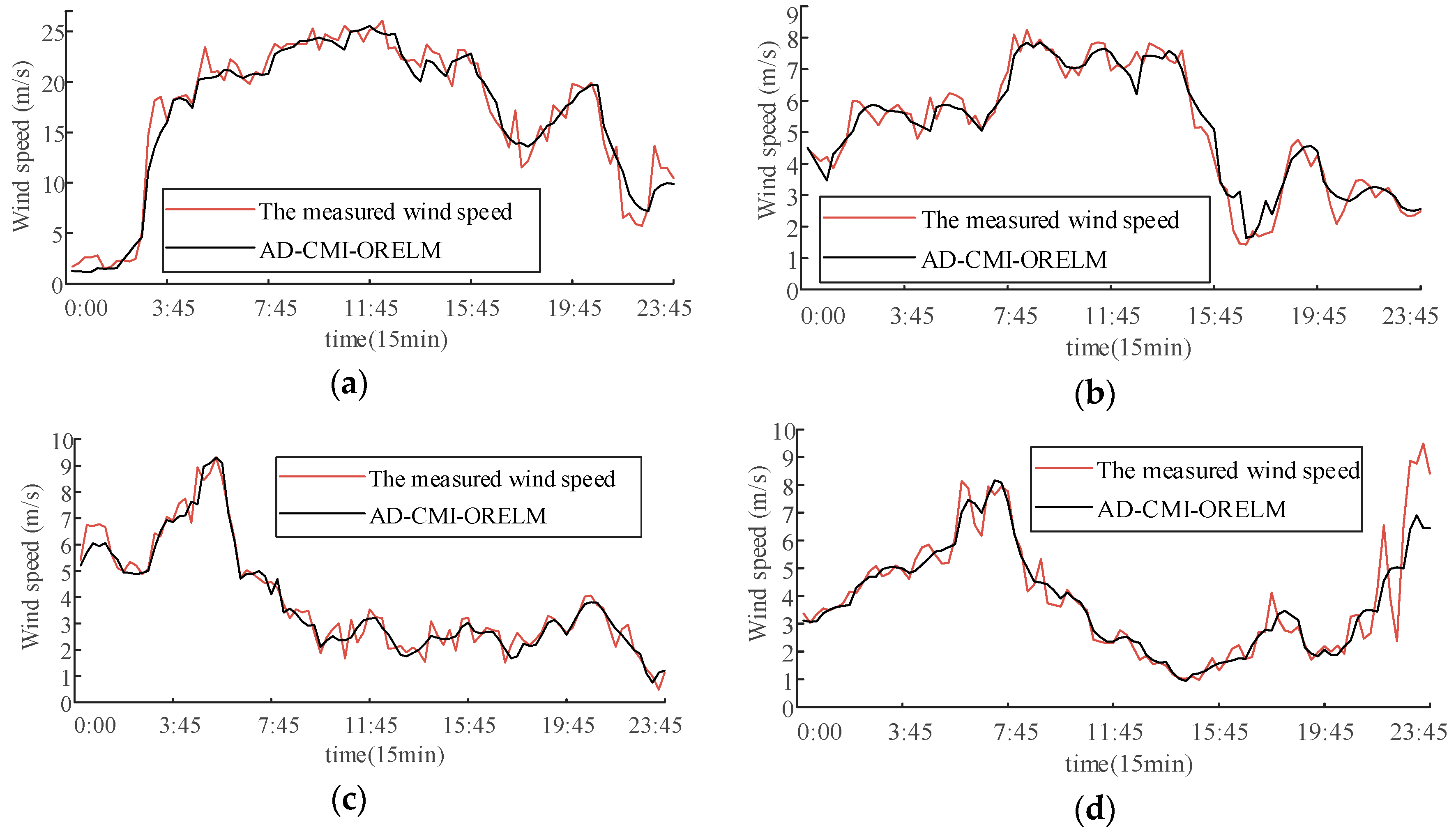
5. Predictive Effect and Model Comparison

In order to verify the effectiveness and advancement of the new method, the optimal feature subset selected by the AD data feature selection is combined with different predictors. Meanwhile, to ensure the comparison results have wider ramifications, Classification and Regression Tree [37] (CART) which can automatically complete the feature selection process according to the training set sample and obtain the optimal feature set is used to predict the wind speed samples of different period of time. Figure 7 shows the prediction curves of the AD-CMI-ORELM method by taking the four predicted days as examples.

On 21 January, Figure 6 shows that the range of wind speed is very wide (minimum 1.55 m/s to 26.07 m/s), and wind speed increased from 2.43 m/s to 18.52 m/s rapidly, which brought extremely high requirement to prediction models. In the other three predicted days, the wind speed was less than 10 m/s and there was a plummet in wind speed. In particular, wind speed on 18 July was up to 17 h in a continuous random fluctuation period below 5 m/s. However, it can be seen from Figure 7 that, although situations of the four predicted days brought challenges to the prediction model, the new method can accurately fit the trend of wind speed, which proves the effectiveness and advancement of the new method.

Table 8. Prediction accuracy on different predict days.

Periods of Time	Analysis Methods	AD-ORELM			AD-ELM			AD-BPNN			AD-CART
		RMSE (m/s)	MAPE	DIM	RMSE (m/s)	MAPE	DIM	RMSE (m/s)	MAPE	DIM	RMSE (m/s)	MAPE	DIM
21 January	PCC	1.7284	11.42%	17	1.8966	12.84%	14	1.7655	12.51%	103	1.6725	11.03%	32
	MI	1.6987	11.33%	17	1.7187	12.52%	21	1.7295	12.44%	118
	CMI	1.5056	10.81%	18	1.6244	12.03%	19	1.7083	12.37%	116
17 April	PCC	0.5545	9.68%	22	0.5655	11.96%	10	0.5097	11.49%	34	0.5261	9.75%	25
	MI	0.5118	9.77%	23	0.5401	11.81%	18	0.6424	11.9%	90
	CMI	0.4545	9.17%	23	0.5005	11.43%	21	0.5024	11.41%	30
18 July	PCC	0.5054	11.54%	17	0.5481	13.22%	16	0.5468	13.43%	24	0.4855	11.09%	27
	MI	0.5021	11.15%	19	0.5476	13.12%	15	0.5015	12.94%	106
	CMI	0.4141	11.06%	19	0.4603	12.74%	17	0.4439	12.66%	44
7 November	PCC	0.4561	10.37%	15	0.4211	11.49%	15	0.4972	12.28%	88	0.372	10.41%	20
	MI	0.3988	10.45%	14	0.453	11.61%	52	0.4484	11.89%	55
	CMI	0.3269	9.72%	15	0.3704	10.95%	15	0.4154	11.52%	59

shows the prediction error of predictors construct with different optimal feature subsets. It can be seen from Table 8 that, no matter in which predicted day, the MAPE and RMSE generated with the optimal feature subset obtained by CMI are significantly less than the ones based on PCC and MI. This indicates that low redundancy feature subset can effectively improve the prediction accuracy of the model.

Models established with ORELM generated lower MAPE and RMSE, which proves that ORELM introduced the specification parameters C and adjusted the target function of ELM effectively reduces the effect of outlier data on the prediction precision and improves the generalization performance of the model.

The comparison experiment proves that the new method can obtain better forecast results than AD-CART method, which once again proved that the performance of feature selection can be improved by using adjacent samples as validation set and the effectiveness of ORELM as a predictor. AD-CMI-ORELM model also obtained the minimum MAPE and RMSE in each prediction day. Take the experimental result of 21 January as an example. The AD-CMI-ORELM model decreased by 15.81% compared with MAPE of the worst model AD-PCC-ELM, while RMSE decreased by 20.6%. AD-CMI-ORELM was reduced by 4.6% and RMSE by 11.4%, compared with the suboptimal model AD-MI-ORELM. There is a similar increase in the other three predicted days, which proves the effectiveness and advancement of the new method. Meanwhile, due to the frequent and larger fluctuation of wind speed on 21 January, the RMSE was slightly worse than that of the other three predicted days.

However, compared with the other methods, the new method still has the same proportion of improvement, which further proves the effectiveness and advancement of the new method.

In order to further illustrate the effectiveness of the new method, the 7-day data was randomly selected from each season in 2009 to constitute a test set and verify the prediction effect of different models. The average error of each model in different seasons is shown in

Table 9. Prediction results on all selected predict days.

Seasons	Analysis Methods	AD-ORELM		AD-ELM		AD-BPNN		AD-CART
		RMSE (m/s)	MAPE	RMSE (m/s)	MAPE	RMSE (m/s)	MAPE	RMSE (m/s)	MAPE
Spring	PCC	1.3397	11.23%	1.3878	11.82%	1.397	12.06%	1.3482	11.16%
	MI	1.3474	11.15%	1.3927	11.79%	1.3856	11.92%
	CMI	1.2881	10.72%	1.3241	11.36%	1.3328	11.17%
Summer	PCC	0.5894	11.32%	0.6633	12.45%	0.6648	12.45%	0.5872	11.3%
	MI	0.5911	11.27%	0.6519	12.40%	0.6467	12.49%
	CMI	0.5321	10.84%	0.5864	11.86%	0.5942	11.89%
Autumn	PCC	0.5290	10.88%	0.5843	11.97%	0.5798	11.98%	0.4957	10.83%
	MI	0.5204	10.95%	0.5774	11.96%	0.5760	12.02%
	CMI	0.4684	10.25%	0.5175	11.28%	0.4995	11.46%
Winter	PCC	0.9491	11.63%	0.9825	12.54%	0.9858	12.89%	0.943	11.25%
	MI	0.9521	11.71%	0.9908	12.75%	0.9832	12.89%
	CMI	0.9026	10.93%	0.9493	12.02%	0.9375	12.27%

.

It can be seen from Table 9 that the error indexes of AD-AMI-ORELM model adopted by the new method still have obvious advantages in the prediction results obtained in all models, and the validity of the new method is proved again.

In order to explain the difference in the prediction performances of different seasons,

Table 10. The statistical indicators of wind speed in different seasons.

Feature	Seasons	Range of Variation	Variance Value
Wind speed	Spring	[0.29, 32.48]	22.34
	Summer	[0.29, 31.57]	10.30
	Autumn	[0.25, 30.52]	7.12
	Winter	[0.25, 32.65]	21.76

presents the statistical indicators of wind speed in different seasons. As shown in Table 10, the range of wind speed is similar in the four seasons, but according to variance value of the wind speed, wind speed in spring and winter is more volatile and violent. Therefore, the RMSE of the new method in spring and winter is higher than that in summer and autumn.

6. Conclusions

To overcome the lack consider of the redundancy between features in the modeling process and the variation of wind speed characteristics at different time periods. This paper makes the following innovations to improve the pertinence and prediction accuracy of wind speed forecasting model:

(1)

A low redundancy feature selection is carried out with the CMI method, which reduced the effect of redundancy between features on prediction accuracy and complexity of a model.

(2)

Building prediction model with ORELM, which improves the generalization performance of the prediction model based on the high prediction efficiency by adding the standard parameter adjustment training error and output layer weight into the target function of ELM.

(3)

The targeted feature selection process and modeling are carried out on different forecast days, overcomes the shortcoming of carrying out feature selection with annual data, which is difficult to show the correlation between wind speed and complex meteorological factors in different time periods, improved the pertinence and prediction of wind speed forecasting model.

The experimental results verified the effectiveness and advancements presented of the new method.

References

1. Men, Z.X.; Yee, E.; Lien, F.S.; Wen, D.Y.; Chen, Y.S. Short-term wind speed and power forecasting using an ensemble of mixture density neural networks. Renew. Energy 2016, 87, 203–211. [Google Scholar] [CrossRef]
2. Ye, L.; Zhao, Y.; Zeng, C.; Zhang, C. Short-term wind power prediction based on spatial model. Renew. Energy 2017, 101, 1067–1074. [Google Scholar] [CrossRef]
3. Wang, H.Z. Deep learning based ensemble approach for probabilistic wind power forecasting. Appl. Energy 2017, 118, 56–70. [Google Scholar] [CrossRef]
4. Jadidoleslam, M.; Ebrahimi, A.; Latify, M.A. Probabilistic Transmission Expansion Planning to Maximize the Integration of Wind Power. Renew. Energy 2017, 114, 866–878. [Google Scholar] [CrossRef]
5. Yin, H.; Dong, Z.; Chen, Y.; Ge, J.; Lai, L.L.; Vaccaro, A.; Meng, A. An effective secondary decomposition approach for wind power forecasting using extreme learning machine trained by crisscross optimization. Energy Convers. Manag. 2017, 150, 108–121. [Google Scholar] [CrossRef]
6. Yuan, X.; Tan, Q.; Lei, X.; Yuan, Y.; Wu, X. Wind Power Prediction Using Hybrid Autoregressive Fractionally Integrated Moving Average and Least Square Support Vector Machine. Energy 2017, 129, 122–137. [Google Scholar] [CrossRef]
7. Wang, J.; Song, Y.; Liu, F.; Hou, R. Analysis and application of forecasting models in wind power integration: A review of multi-step-ahead wind speed forecasting models. Renew. Sustain. Energy Rev. 2016, 60, 960–981. [Google Scholar] [CrossRef]
8. Ssekulima, E.B.; Anwar, M.B.; Al Hinai, A.; El Moursi, M.S. Wind speed and solar irradiance forecasting techniques for enhanced renewable energy integration with the grid: A review. IET Renew. Power Gener. 2016, 10, 885–989. [Google Scholar] [CrossRef]
9. Zhao, J.; Wang, J.; Liu, F. Multistep Forecasting for Short-Term Wind Speed Using an Optimized Extreme Learning Machine Network with Decomposition-Based Signal Filtering. J. Energy Eng. 2016, 142, 04015036. [Google Scholar] [CrossRef]
10. Guo, Z.; Zhao, W.; Lu, H.; Wang, J. Multi-step forecasting for wind speed using a modified EMD-based artificial neural network model. Renew. Energy 2012, 37, 241–249. [Google Scholar] [CrossRef]
11. Chen, D.; Lin, J.; Li, Y. Modified complementary ensemble empirical mode decomposition and intrinsic mode functions evaluation index for high-speed train gearbox fault diagnosis. J. Sound Vib. 2018, 424, 192–207. [Google Scholar] [CrossRef]
12. Niu, M.; Wang, Y.; Sun, S.; Li, Y. A novel hybrid decomposition-and-ensemble model based on CEEMD and GWO for short-term PM 2.5, concentration forecasting. Atmos. Environ. 2016, 134, 168–180. [Google Scholar] [CrossRef]
13. Wang, Y.W.; Feng, L.Z. A new feature selection method for handling redundant information in text classification. Front. Inf. Technol. Electron. Eng. 2018, 19, 221–234. [Google Scholar] [CrossRef]
14. Wang, Y.; Feng, L. Hybrid feature selection using component co-occurrence based feature relevance measurement. Expert Syst. Appl. 2018, 102, 83–99. [Google Scholar] [CrossRef]
15. Lin, Y.; Hu, Q.; Liu, J.; Li, J.; Wu, X. Streaming Feature Selection for Multilabel Learning Based on Fuzzy Mutual Information. IEEE Trans. Fuzzy Syst. 2017, 25, 1491–1507. [Google Scholar] [CrossRef]
16. Li, S.; Wang, P.; Goel, L. A Novel Wavelet-Based Ensemble Method for Short-Term Load Forecasting with Hybrid Neural Networks and Feature Selection. IEEE Trans. Power Syst. 2016, 31, 1788–1798. [Google Scholar] [CrossRef]
17. Liu, D.; Wang, J.; Wang, H. Short-term wind speed forecasting based on spectral clustering and optimised echo state networks. Renew. Energy 2015, 78, 599–608. [Google Scholar] [CrossRef]
18. Feng, C.; Cui, M.; Hodge, B.M.; Zhang, J. A data-driven multi-model methodology with deep feature selection for short-term wind forecasting. Appl. Energy 2017, 190, 1245–1257. [Google Scholar] [CrossRef]
19. Hu, Q.; Su, P.; Yu, D.; Liu, J. Pattern-Based Wind Speed Prediction Based on Generalized Principal Component Analysis. IEEE Trans. Sustain. Energy 2014, 5, 866–874. [Google Scholar] [CrossRef]
20. Poncela, M.; Poncela, P.; Perán, J.R. Automatic tuning of Kalman filters by maximum likelihood methods for wind energy forecasting. Appl. Energy 2013, 108, 349–362. [Google Scholar] [CrossRef]
21. Erdem, E.; Shi, J. ARMA based approaches for forecasting the tuple of wind speed and direction. Appl. Energy 2011, 88, 1405–1414. [Google Scholar] [CrossRef]
22. Ma, X.; Jin, Y.; Dong, Q. A generalized dynamic fuzzy neural network based on singular spectrum analysis optimized by brain storm optimization for short-term wind speed forecasting. Appl. Soft Comput. 2017, 54, 296–312. [Google Scholar] [CrossRef]
23. Gouveia, H.T.; de Aquino, R.R.; Ferreira, A.A. Enhancing Short-Term Wind Power Forecasting through Multiresolution Analysis and Echo State Networks. Energies 2018, 11, 824. [Google Scholar] [CrossRef]
24. Bonanno, F.; Capizzi, G.; Sciuto, G.L. A neuro wavelet-based approach for short-term load forecasting in integrated generation systems. In Proceedings of the International Conference on Clean Electrical Power, Alghero, Italy, 11–13 June 2013; pp. 772–776. [Google Scholar]
25. Chen, Y.; Cai, K.; Tu, Z.; Nie, W.; Ji, T.; Hu, B.; Chen, C.; Jiang, S. Prediction of benzo[a]pyrene content of smoked sausage using back-propagation artificial neural network. J. Sci. Food Agric. 2018, 98, 3022–3030. [Google Scholar] [CrossRef] [PubMed]
26. Noorollahi, Y.; Jokar, M.A.; Kalhor, A. Using artificial neural networks for temporal and spatial wind speed forecasting in Iran. Energy Convers. Manag. 2016, 115, 17–25. [Google Scholar] [CrossRef]
27. Huang, G.B.; Zhu, Q.Y.; Siew, C.K. Extreme learning machine: Theory and applications. Neurocomputing 2006, 70, 489–501. [Google Scholar] [CrossRef] [Green Version]
28. Zhang, K.; Luo, M. Outlier-robust extreme learning machine for regression problems. Neurocomputing 2015, 151, 1519–1527. [Google Scholar] [CrossRef]
29. Huang, N.E.; Shen, Z.; Long, S.R.; Wu, M.C.; Shih, H.H.; Zheng, Q.; Yen, N.C.; Tung, C.C.; Liu, H.H. The empirical mode decomposition and the Hilbert spectrum for nonlinear and non-stationary time series analysis. Proc. Math. Phys. Eng. Sci. 1998, 454, 903–995. [Google Scholar] [CrossRef]
30. Yeh, J.R.; Shieh, J.S.; Huang, N.E. Complementary ensemble empirical mode decomposition: A novel noise enhanced data analysis method. Adv. Adapt. Data Anal. 2010, 2, 135–156. [Google Scholar] [CrossRef]
31. Cover, T.M.; Thomas, J.A. Elements of Information Theory; John Wiley & Sons: New York, NY, USA, 1991; pp. 155–183. [Google Scholar]
32. Peng, X.; Zheng, W.; Zhang, D.; Liu, Y.; Lu, D.; Lin, L. A novel probabilistic wind speed forecasting based on combination of the adaptive ensemble of on-line sequential ORELM (Outlier Robust Extreme Learning Machine) and TVMCF (time-varying mixture copula function). Energy Convers. Manag. 2017, 138, 587–602. [Google Scholar] [CrossRef]
33. Li, H.; Zhou, M.; Guo, Q.; Wu, R.; Xi, J. Compressive sensing-based wind speed estimation for low-altitude wind-shear with airborne phased array radar. Multidimens. Syst. Signal Process. 2016, 7, 1–14. [Google Scholar] [CrossRef]
34. Groves, G.V. Determination of Air Density Temperature & Winds at High Altitudes; University Coll: London, UK, 1966. [Google Scholar]
35. NWTC Information Portal. Available online: http://wind.nrel.gov/MetData/ (accessed on 15 June 2018).
36. Mu, Y.; Liu, X.; Wang, L. A Pearson’s correlation coefficient based decision tree and its parallel implementation. Inf. Sci. 2018, 435, 40–58. [Google Scholar] [CrossRef]
37. Huang, N.; Peng, H.; Cai, G.; Chen, J. Power Quality Disturbances Feature Selection and Recognition Using Optimal Multi-Resolution Fast S-Transform and CART Algorithm. Energies 2016, 9, 927. [Google Scholar] [CrossRef]
Figure 1. The geographical location of date measurement in NWTC.
Energies 11 01638 g001
Figure 2. Wind speed curves reconstructed by different decomposition methods.
Energies 11 01638 g002
Figure 3. Prediction of data set construction on 6 April 2009.
Energies 11 01638 g003
Figure 4. Average weekly error curves with different parameter k.
Energies 11 01638 g004
Figure 5. Results of the features’ correlation analysis. (a) The correlation analysis results on 21 January; (b) The correlation analysis results on 17 April; (c) The correlation analysis results on 18 July; (d) The correlation analysis results on 7 November; (e) The correlation analysis results of the whole year.
Energies 11 01638 g005aEnergies 11 01638 g005b
Figure 6. Optimal feature selection curves. (a) Analysis curves with AD data; (b) Analysis curves with YD data.
Energies 11 01638 g006aEnergies 11 01638 g006b
Figure 7. Predicts curves of the proposed method on different predict days (a) Forecast curve of 21 January; (b) Forecast curve of 17 April; (c) Forecast curve of 18 July; (d) Forecast curve of 7 November.
Energies 11 01638 g007