1. Introduction
Conditional volatility models are the most widely estimated univariate and multivariate models of time-varying volatility (or dynamic risk) applied to financial data, in the high frequency data domains that are measured in days, hours and minutes. The stochastic processes, regularity conditions and asymptotic properties of these popular univariate conditional volatility models, such as GARCH (see Engle [
1] and Bollerslev [
2]) and GJR (see Glosten and Runkle [
3]), are well established in the literature. Nevertheless, McAleer and Hafner [
4] raised caveats about the existence of the stochastic process and statistical properties underlying exponential GARCH (EGARCH) (see [
5,
6]).
The situation with respect to multivariate conditional volatility models is considerably different. For example, the Full BEKK model, (see Baba and [
7], and Engle and Kroner [
8]) is subject to uncertainty regarding the existence of its underlying stochastic processes, regularity conditions, and asymptotic properties. These properties have either not yet been established, or are simply assumed rather than derived, yet these conditions and properties are essential for the existence of the likelihood function, and hence valid statistical analysis of the empirical estimates. This means that when the model is estimated its coefficients and statistical properties are subject to uncertainty and may not be valid. These limitations do not apply to the DBEKK model, which is used as a benchmark in this study.
The focus of this paper is to explore the potential and empirical biases that may exist in the typical estimation of the multivariate Full BEKK model, as referenced in the Rats statistical software (Estima 1560 Sherman Ave, Suite 1029 Evanston, IL 60201, USA).
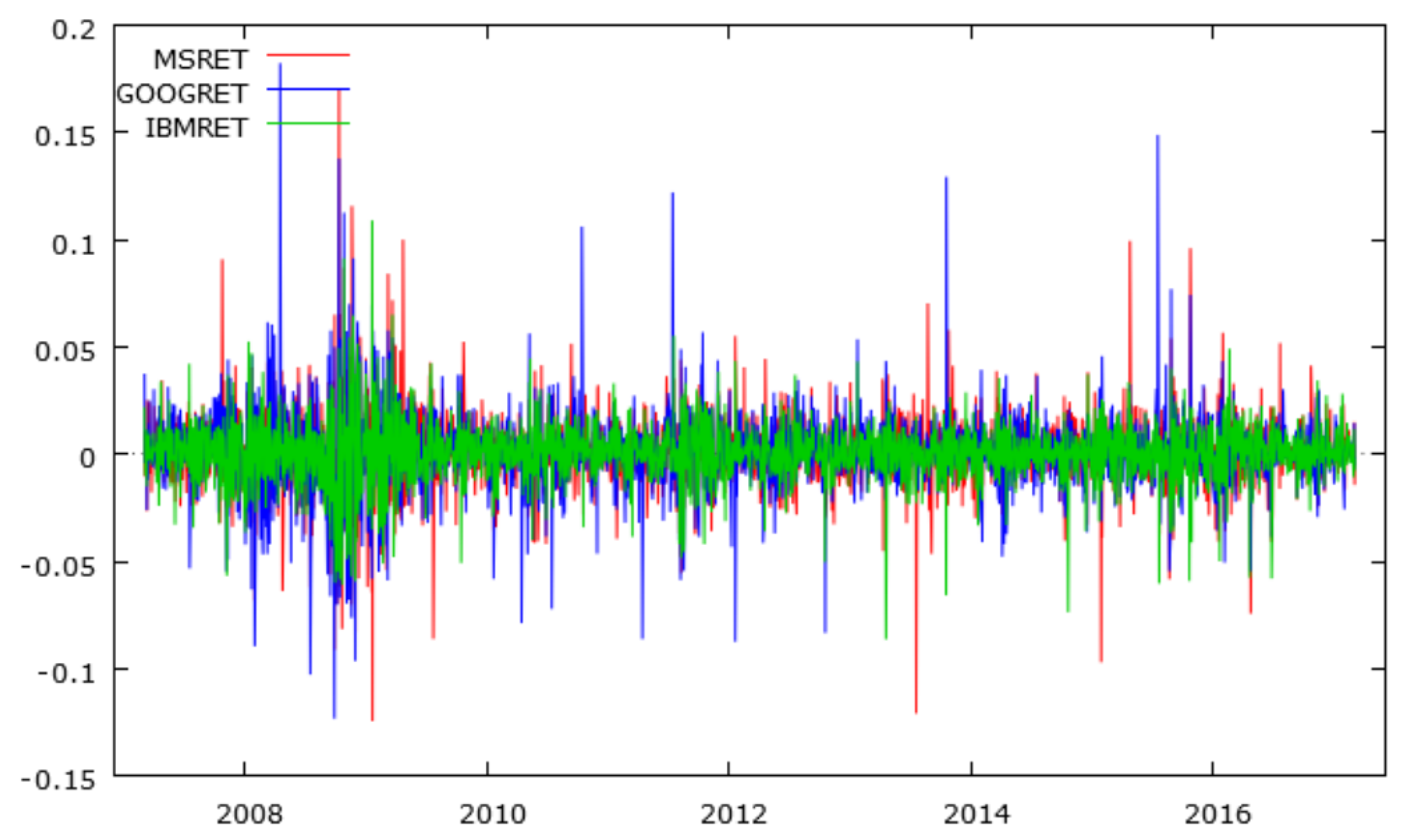
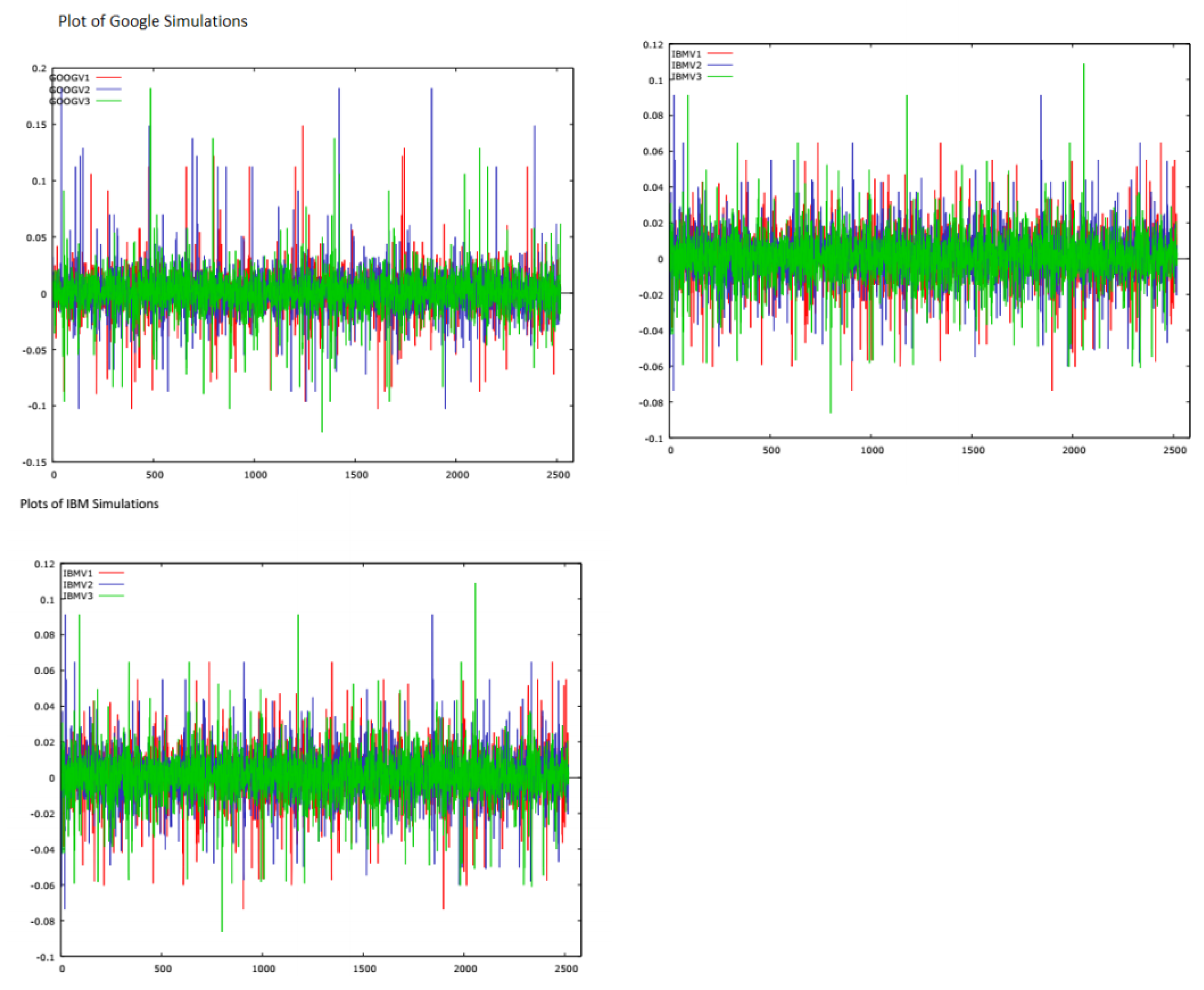
We use three simulated sets of daily returns derived from ten years of daily data, from 5 March 2007 to 3 March 2017, for Google , IBM and Microsoft. (Data accessed on 6 March 2017, in Perth, Western Australia). The original adjusted return series were downloaded from Yahoo Finance. The random simulations, created in R, are done in blocks, including five lags so as to preserve autocorrelations and ARCH effects. We use the estimated coeffcients of the conditional variances and conditional covariances derived from Diagonal BEKK (DBEKK), which has appropriate regularity conditions and statistical properties, as the benchmark.
McAleer and Lieberman [
9] showed that the QMLE of the parameters of DBEKK models are consistent and asymptotically normal, so that standard statistical inference for testing hypotheses is valid. These are compared with estimates of the same coefficients using the Full BEKK model. Non-parametric tests reveal statistically significant bias in the Full BEKK coefficient estimates for the conditional variances and covariances.
Engle and Kroner [
8], in their original extended discussion of multivariate ARCH models, suggest that: “Very little is currently known about the properties of maximum likelihood estimators in univariate GARCH models, let alone in multivariate GARCH-in-mean models, despite the fact that this estimator permeates the multivariate GARCH-in-mean literature”. This issue is a central focus of the current paper, which is developed from the fact that, in the current extant literature, the relevant statistical properties required for the estimation of full BEKK models are assumed rather than proven. This is not the case for the DBEKK model, so we apply the former as a lense, which can be used to assess potential biases in the latter, the BEKK model.
It is important, for both investment purposes and in the interests of informed financial policy making, that any limitations and biases in the estimation and application of the BEKK model are understood. In practice, the model is frequently utilised. For example, in recent studies, Gounopoulos [
10] used a BEKK model to examine linkages between stock returns and currency exposures of a sample of US, UK, and Japanese banks and insurance companies. Long and Zhang [
11], similarly apply a BEKK model to analyze the conditional time-varying currency betas in five developed and six emerging financial markets. Caporale and Spagnolo [
12] test the impact of exchange rate uncertainty on net equity and net bond flows and on their dynamic linkages applying a BEKK model. Cardona and Agudelo [
13] use a BEKK model to explore volatility transmission effects between US and Latin American financial markets.
The paper is divided into four sections. The introductory section is followed by
Section 2, which describes the data sets, their statistical characteristics, and the models and empirical methods used.
Section 3 presents the empirical results, and
Section 4 provides some concluding remarks.
3. Empirical Results
We estimated both DBEKK and Full BEKK using the simulated financial return series. The estimates from DBEKK are used as the benchmark, given that it has established statistical regularity conditions. We decided to keep the comparison tests as simple as possible and first estimated a two-variable version of the DBEKK and Full BEKK models using the the three sets of simulated return series in pairs. This was then followed by a single three-variable set of estimates, in order to verify that the same pattern of results exists. The null hypothesis is that Diagonal and Full BEKK are equivalent when the off-diagonal coefficients in Full BEKK are zero, so the asymptotic tests are statistically valid. We proceeded by estimating the coefficients for the conditional variances and the conditional covariances for the two models, and then used non-parametric sign tests on the differences between the two sets of estimates.
The estimates of the constants, ARCH effects and conditional variances for the two models are shown in
Table 4. DBEKK and Full BEKK fitted to the pairs of simulated series were highly significant, and all but three pairs of the fifty-four coefficients estimated in the models, and presented in
Table 4, were significant at the 1% level. (The insignificant coefficients are marked with an asterisk ( *) in
Table 4.) The coefficients of the conditional covariances are shown in
Table 5. The majority of these estimates are insignificant, so we concentrated our analysis on the conditional variances.
We then undertook a set of non-parametric sign tests on the values of the estimated coefficients, reported in
Table 4. We ran the tests in a number of different formats, both on the full set of coefficients reported in
Table 4, and the full set minus the three pairs of insignificant estimates. The results of the sign tests are reported in
Table 6 and
Table 7, which suggest that there are no significant differences in the values of the coefficients for the constants, ARCH effects and the conditional variances estimated for the two variables. However, these tests treat the coefficients in isolation, and regard them as being independent, which is not the case when they are combined into a DBEKK or Full BEKK model.
DBEKK and Full BEKK are multivariate GARCH models that are used for forecasting conditional volatility. The crucial issue for purposes of risk management is how the forecasts of conditional volatility derived from the two models compare. These are vital components for assessing risk, and might be used to compute the Value at Risk (VaR) of a portfolio of financial assets, for example.
The simulated financial return samples for the nine variables contain ten years of daily data, or 2581 data points. We filter these through the DBEKK and Full BEKK models, and obtain corresponding estimates of the conditional variance projections, for each simulated security, from the two models. These forecasts of the conditional variances are then compared using non-parametric sign tests. The results for each simulated security are shown in
Table 8.
The sign tests in
Table 8 are based on the null hypothesis that the median difference in the conditional variances produced by the two models, DBEKK and Full BEKK, for the simulated securities, is zero. The null hypothesis is strongly rejected in all cases, and the differences are highly significant. We also ran sign tests, not reported, based on the null hypothesis that there was no difference in the conditional variances predicted by the two models. These results also strongly rejected the null hypothesis in all cases.
While it is valuable to know that the two models produce different predictions of the conditional variances, it is also of interest to know whether or not there are
systematic differences in the predictions of the conditional variances. We explore this issue by means of quantile regression. The advantage of quantile regression is that we can explore the relationship between the two sets of predictions from DBEKK and Full BEKK at particular quantiles. We regress the predicted conditional variances from the Full BEKK model on the corresponding predictions from DBEKK for each of the simulated securities, in the pairs of securities modelled. We treat the predictions of conditional variances from the Full BEKK model as the dependent variable. The results of these quantile regressions are shown in
Table 9.
Table 9 reveals a distinct pattern of an increase in the slope coefficients as we move across the quantiles from the lowest 0.05 quantile to the highest 0.95 quantile. The most extreme case is the prediction of the conditional variances for the relationship between IBMV2 and MSV2. In the 0.05 quantile, the conditional variance prediction by Full BEKK is 50 times lower than for DBEKK, and, in the 0.095 quantile, it is 18 times higher (though there were convergence issues encountered in the Full BEKK estimation in this case). Even so, the difference across these two extreme quantiles usually varies by between 10 and 20 percent. This is still very large if we intend to use the models to predict a portfolio VAR.
If we use the predictions of DBEKK as the benchmark, then application of the Full BEKK model to the same data set may underestimate risk in the lowest quantile and overestimate risk in the highest quantile. In the eighteen examples, seven of the total estimates suggest risk in the 0.05 quantile will be lower by 10 percent or more when estimated by Full BEKK, as opposed to DBEKK. Similarly, in nine of the total cases, the estimate of risk in the 0.095 quantile is 10 percent or more, when estimated by Full BEKK, as compared with DBEKK. Thus, there are considerable discrepancies in the predictions of conditional volatility based on these applications of the two models.
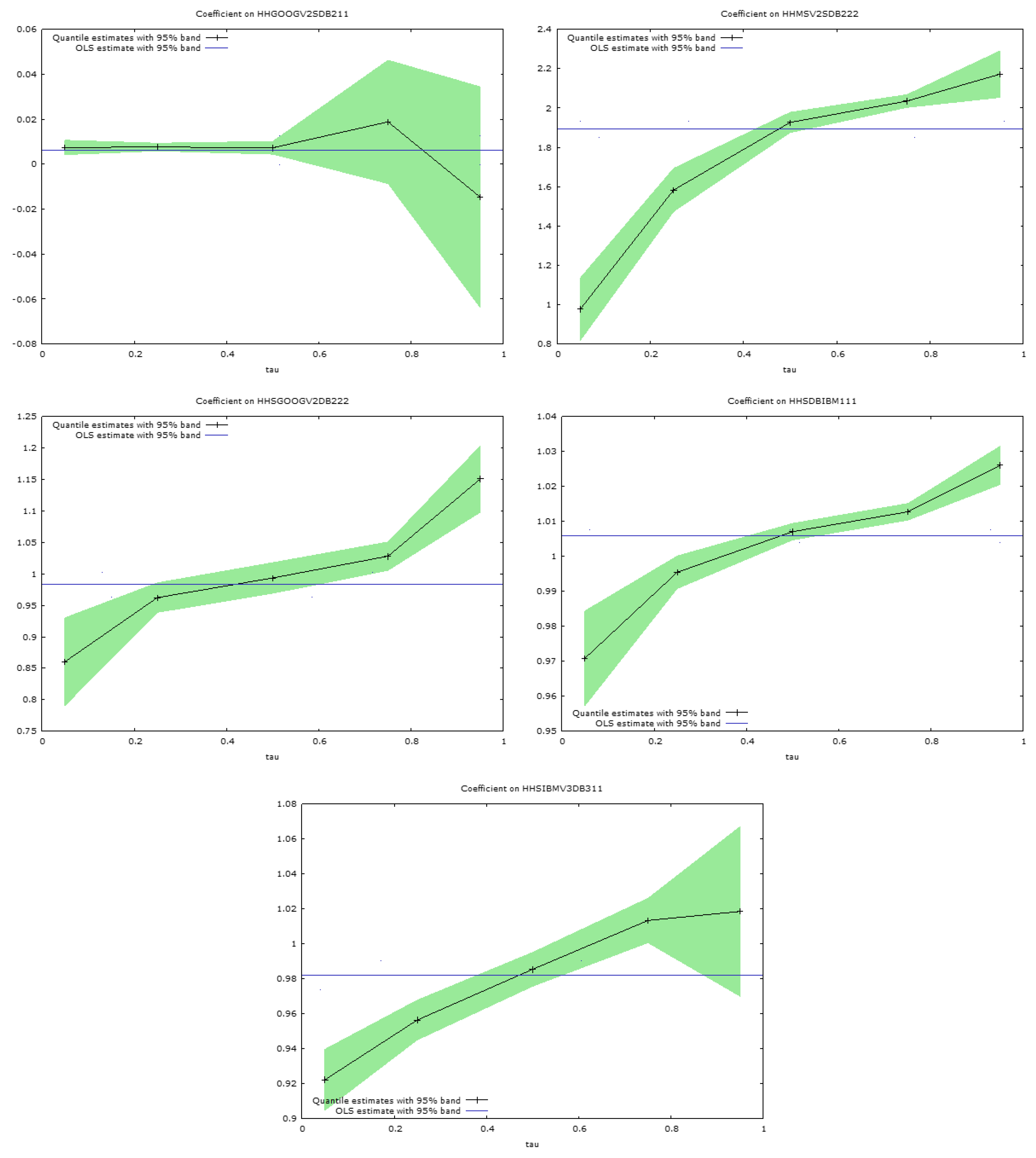
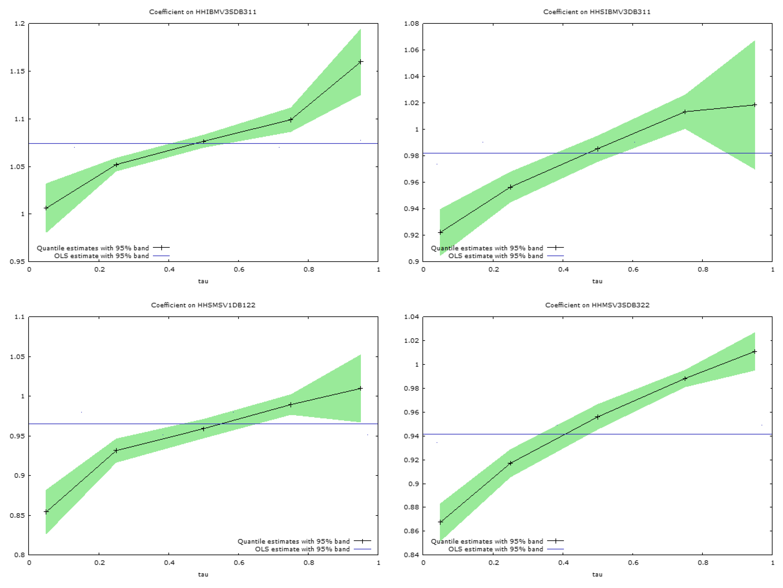
These discrepancies in the regression slope coefficients are apparent in
Figure 5 and
Figure 6, which present graphs of the estimated slope coefficients across the quantiles for the pairs of simulated securities considered. The quantile regression bounds estimated at the 0.95 level are shown around the quantile slope estimates in each figure. The horizontal lines, in the centre of the figures, show the ordinary least squares regression slopes for the regressions of conditional variances for each security, regressed on the conditional variances for the same security, when considered in the same pairwise estimates produced by DBEKK. The ordinary least squares slope coefficients are not very informative, and merely suggest whether the predicted conditional variances from Full BEKK are relatively above or below those from DBEKK. There is considerable variation in the figures, but most of them are slightly below one.
The quantile regression analyses are much more informative. The lines in
Figure 5 and
Figure 6 link the slope coefficients estimated at the 0.05, 0.25, 0.50, 0.75, and 0.95 quantiles, when the predictions of the conditional variances from Full BEKK are regressed on those from DBEKK (
Figure 6). In all cases, except for one, shown in
Figure 5 and
Figure 6, the estimates at the lowest 0.05 quantile reveal a relationship between the two sets of estimates that is markedly different from that suggested by ordinary least squares, which captures the average relationship. The relationship is markedly different, at this quantile, frequently by ten to twenty percent.
Another startling feature is that all the slopes depicted in
Figure 5 and
Figure 6 are strongly positive, in that the estimated slope coefficients all increase, with one exception, from the lowest to the highest quantile. Thus, the conditional variances estimated from the Full BEKK model, are much higher, at the 0.95 quantile, often by 20 percent or more, than the conditional variance estimated by the DBEKK model.
These results have strong implications if we try use the two multivariate models to estimate portfolio risk. The analysis reported in the paper, on these simulated financial return series, suggests that the use of the Full BEKK model will underestimate conditional variances in the left-hand tail of the portfolio return distribution, relative to DBEKK, and overestimate it in the right-hand tail of the distribution.
These results are subject to certain caveats. We have estimated the models using the Estima Rats econometric package, and used the default settings when fitting the models. We have not changed any of the tolerances in the algorithms used to fit the models, or changed the settings for the initialization of the algorithms used to commence the models. We have also instructed the program to use the BHHH optimization procedure to fit the models. All the models have been fitted using a Gaussian distribution, and the estimates would be different if we used a t-distribution. (We also did some analysis using the t-distribution, which is not reported in the paper, that revealed a virtually identical pattern of relationships across the quantiles to those that that are reported in the paper). The intention was to use a consistent approach to the fitting of the models and then to explore the consistency of the results.
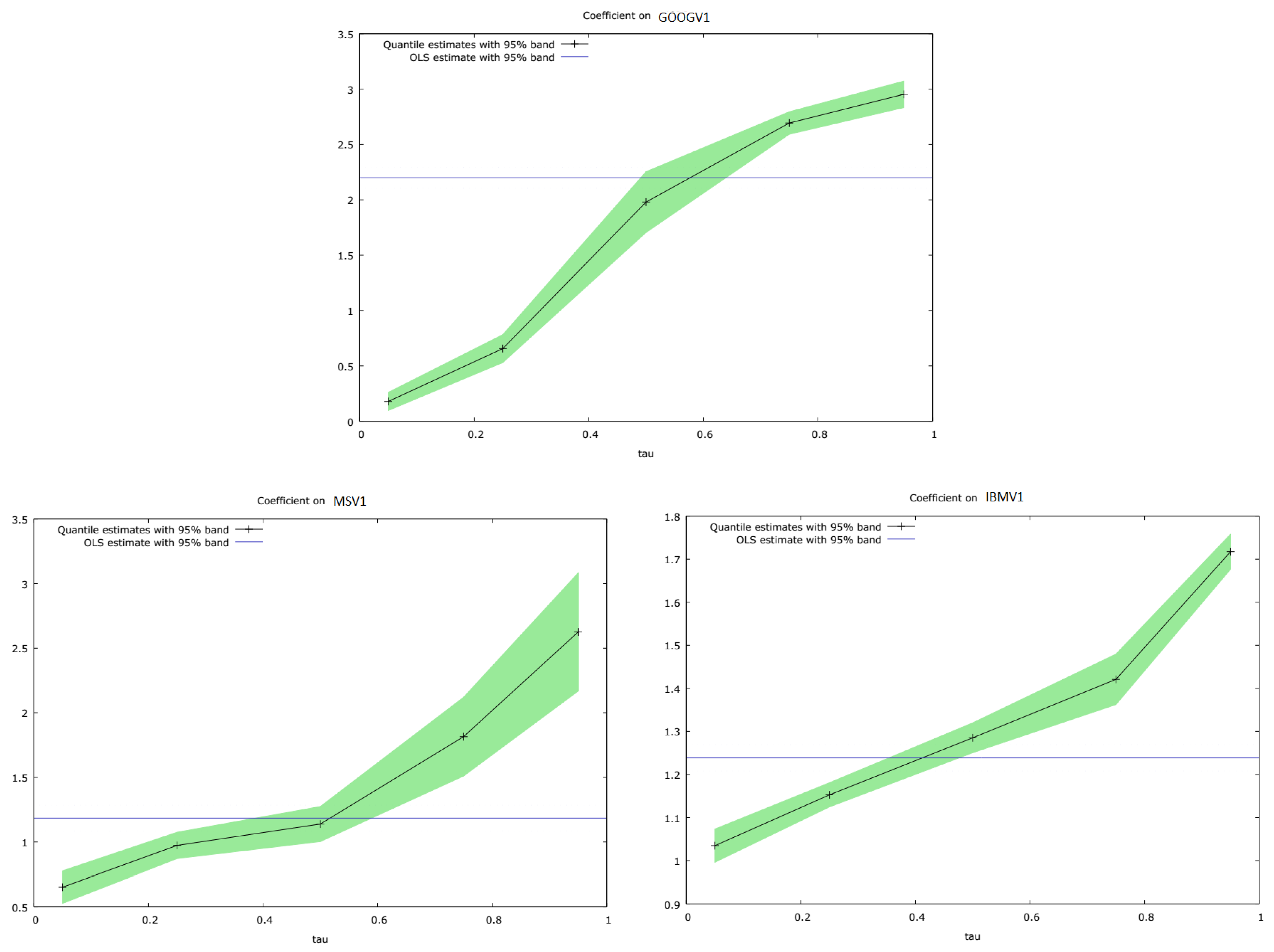
We also estimated DBEKK and Full BEKK using three variables jointly, in this case, GOOGV1, IBMV1, and MSV1, just to check that similar behaviour was displayed when we employed a trivariate estimation procedure. The results are shown in
Table 10.
It is evident in
Table 10 that many of the additional terms included in the Full BEKK model are not statistically significant, at least in this simulated data set. We also ran a quantile regression analysis of the conditional variances produced by Full BEKK, regressed on the conditional variances producd by DBEKK, using these three securities. The results are shown in
Table 11. Plots of the quantile regression slope coefficients are shown in
Figure 7.
It can be seen in
Table 11 and in
Figure 7, respectively, that exactly the same pattern of results emerges, when we estimate DBEKK and Full BEKK on three securities jointly, as previously the case with pairs of securities. The conditional variance estimates for Full BEKK, relative to DBEKK, are comparatively lower in the 0.05 quantile, increase across the quantiles, and are relatively higher in the 0.95 quantile. If the estimates were the same, the slope coefficient would be unity.
We used the DBEKK model as a benchmark, given that the statistical properties of this model have been established. The results, using this benchmark, suggest that there is an observable and relative bias in the predictions of the conditional variances from the Full BEKK model. This has serious practical implications about the use of Full BEKK for risk management and modelling purposes.


