A Novel Hybrid Interval Prediction Approach Based on Modified Lower Upper Bound Estimation in Combination with Multi-Objective Salp Swarm Algorithm for Short-Term Load Forecasting

Abstract

Effective and reliable load forecasting is an important basis for power system planning and operation decisions. Its forecasting accuracy directly affects the safety and economy of the operation of the power system. However, attaining the desired point forecasting accuracy has been regarded as a challenge because of the intrinsic complexity and instability of the power load. Considering the difficulties of accurate point forecasting, interval prediction is able to tolerate increased uncertainty and provide more information for practical operation decisions. In this study, a novel hybrid system for short-term load forecasting (STLF) is proposed by integrating a data preprocessing module, a multi-objective optimization module, and an interval prediction module. In this system, the training process is performed by maximizing the coverage probability and by minimizing the forecasting interval width at the same time. To verify the performance of the proposed hybrid system, half-hourly load data are set as illustrative cases and two experiments are carried out in four states with four quarters in Australia. The simulation results verified the superiority of the proposed technique and the effects of the submodules were analyzed by comparing the outcomes with those of benchmark models. Furthermore, it is proved that the proposed hybrid system is valuable in improving power grid management.

1. Introduction

Load forecasting is of upmost significance and affects the construction and operation of power systems. In the preparation of the power system planning stage, if the load forecasting result is lower than the real demand, the installed and distribution capacities of the planned power system will be insufficient. The power generated will not be able to meet electricity demand of the community it serves, and the entire system will not be able to operate in a stable manner. Conversely, if the load forecast is too high, it will result in power generation, transmission, and distribution, at a larger scale, that cannot be fully used in the real power system. The investment efficiency and the efficiency of the resource utilization will be reduced in this situation. Therefore, effective and reliable power load forecasting can promote a balanced development of the power system while improving the utilization of energy. There are various power load forecasting methods and, commonly, load forecasting is classified into short-term, medium-term, and long-term, based on the application field and forecasting time. Among these categories, short-term load forecasting (STLF) is an essential tool for the planning and operation [1,2] of energy systems and it has thus been a major area of research during the past few decades.

According to existing research, concern mostly focuses on the point forecasting of STLF. Additionally, the relative algorithms can be mainly classified into three major categories: traditional statistical techniques, computational intelligent methods, and multimodule hybrid models [3].

In the early stages of research, traditional statistical techniques were extensively employed for point forecasting of STLF, such as linear regression methods [4,5], exponential smoothing [6], Kalman filters [7], and other linear time-series models. In general, most of the traditional statistical approaches have been involved in linear analysis and have mainly considered linear factors in time series. However, the short-term load series are a mixture of multiple components which include linear and non-linear factors. Therefore, the traditional statistical approaches encounter difficulties when dealing with the STLF, and the forecasting accuracy is often unsatisfactory. With the development of machine learning and artificial intelligence, an increased number of non-linear computational intelligent methods have been applied to STLF, such as neural network models (NN) [8,9], expert systems [10] and support vector machines (SVM) [11,12]. These approaches have been proved to have advantages in dealing with the non-linear problems of STLF compared to traditional statistical methods, thereby eliciting improved performances in most cases. Most importantly, a key point that influences the performance of computational intelligent methods is the setting of related parameters in algorithms. At this time, efficient hybrid models appeared. In hybrid models, different modules were introduced to improve the performance and accuracy of STLF [13,14,15,16,17,18,19]. Among existing reviews in the literature, two popular and efficient modules include the data preprocessing and optimization modules. In the case of the data preprocessing modules, a multiwavelet transform was used in combination with a three-layer feed-forward neural network to extract the training data and predict the load in [13]. Fan et al. [14] used empirical mode decomposition (EMD) to decompose electric load data, generating high-frequency series and residuals for the forecasting of support vector regression (SVR) and autoregression (AR), respectively. The results showed that the hybrid methods can perform well by eliciting good forecasting accuracy and interpretability. In the case of the optimization modules, AlRashidi et al. [15] employed the particle swarm optimizer (PSO) to fine-tune the model parameters, and the forecasting problem was presented in a state space form. Wang et al. [16] proposed a hybrid forecasting model combining differential evolution (DE) and support vector regression (SVR) for load forecasting, where the DE algorithm was used to choose the appropriate parameters for SVR.

However, as mentioned above, the current research on STLF mainly concentrates on point forecasting in which the accuracy is usually measured by the errors between the predicted and the target values. With power system growth and the increase in its complexity, point forecasting might not be able to provide adequate information support for power system decision making. An increasing number of factors, such as load management, energy conversion, spot pricing, independent power producers and non-conventional energy, make point forecasting undependable in practice. In addition to the fact that most of these point forecasting models do not elicit the required precision, they are also not adequately robust. They fail to yield accurate forecasts when quick exogenous changes occur. Other shortcomings are related to noise immunity, portability, and maintenance [20].

In general, point forecasting cannot properly handle uncertainties associated with load datasets in most cases. To avoid such imperfection, interval prediction (IP) of STLF is an efficient way to deal with the forecast uncertainty in electrical power systems. Prediction intervals (PIs) not only provide a range in which targets are highly likely to be covered, but they also provide an indication of their accuracy, known as the coverage probability. Furthermore, the PIs can take into account more uncertain information and the result of (PIs) commonly form a double output (upper bounds and lower bounds) which can reflect more uncertain information and provide a more adequate basis for power system planning.

With the development of artificial intelligence technology, the interval prediction methods based on NN have been proved to be efficient techniques. According to existing research, the popular techniques for constructing PIs are Bayesian [21], delta [22], bootstrap [23], and mean–variance estimation [24]. In the literature, the Bayesian technique [25] is used for the construction of NN-based PIs. Error bars are assigned to the predicted NN values using the Bayesian technique. Even if the theories are effective in the construction of PIs, the calculation of the Hessian matrix will result in the increase of model complexity and computation cost. In [26], the delta technique was applied to construct PIs for STLF, and a simulated annealing (SA) algorithm was introduced to improve the performance of PIs through the minimization of a loss function. In [27], according to bootstrap, error output, resampling, and multilinear regression, were used with STLF for the construction of confidence intervals with NN models. In [24], a mean–variance estimation-based method used NN to estimate the characteristics of the conditional target distribution. Additive Gaussian noise with non-constant variance was the key assumption of the method for PI construction.

Considering most of the existing research studies of PIs by NN mentioned above, the PIs were usually calculated depending on the point forecasting. The NNs were first trained by minimizing an error-based cost function, and the PIs were then constructed depending on the outcomes of trained and tuned NNs. It may be questionable to construct PIs in this way. Furthermore, it is a more reasonable way to output the upper and lower bounds directly [28]. Compared with the Bayesian, delta, and bootstrap techniques, this approach can output the PIs without being dependent on point prediction. However, in traditional research approaches, the cost function mainly aims at guaranteeing coverage probability (CP). However, a satisfactory coverage probability can be achieved easily by assigning sufficiently large and small values to the upper and lower bounds of the PIs. Thus, the prediction interval width (PIW) is another key characteristic which needs to be considered fully. These two goals, that is, achieving a higher CP and a lower PIW, should be considered in a comprehensive manner when the NN parameters are determined.

Therefore, in this study, a hybrid, lower upper bound estimation (LUBE) based on multi-objective optimization is proposed. The requirements for higher CP and lower PIW constitute a typical case of the Pareto optimization problem. In the present study, a significant and valid approach was used to solve the Pareto optimization problem is the multi-objective optimization [29]. There are many algorithms in the literature for solving multi-objective optimizations. For the GA, the most well-regarded multi-objective algorithm is the non-dominated sorting genetic algorithm (NSGA) [30]. Other popular algorithms include the multi-objective particle swarm optimization (MOPSO) [31,32], multi-objective ant colony optimization (MOACO) [33], multi-objective differential evolution (MODE) [34], multi-objective grasshopper optimization (MOGO) [35], multi-objective evolution strategy (MOES) [36], multi-objective sine cosine (MOSC) [37], and multi-objective ant lion [38]. All these algorithms are proved to be effective in identifying non-dominated solutions for multi-objective problems. According to the “no free lunch theorem” for optimization [39,40], there is no algorithm capable of solving optimization algorithms for all types of problems. This theorem logically proves this and proposes new algorithms, or improves the current ones.

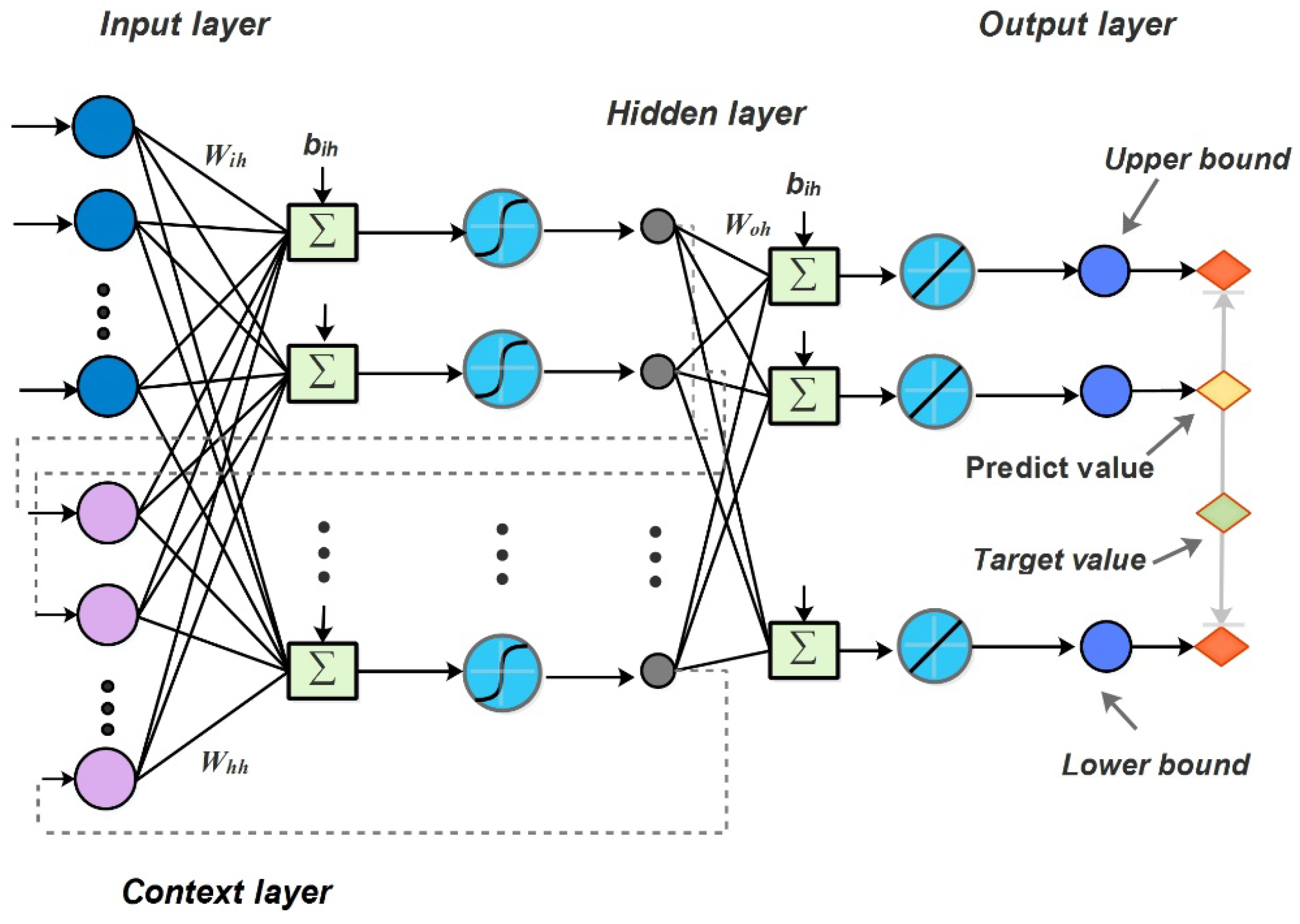
In this study, to achieve a better performance in STLF, one of the novel recurrent neural networks, the Elman neural network (ENN) [41], is applied to construct the structure of a modified LUBE. The Elman neural network has already been extensively used in time-series forecasting [42,43,44]. As a type of recurrent neural network, ENN exhibits superiority on the time delay information because of the existence of the undertaking layer which can connect hidden NN layers and store the historical information in the training process. This structure design of NN commonly leads to a better performance in time-series forecasting.

In traditional STLF, most of the methods construct the training set of the model directly using the original data. However, data in the natural world often receives a lot of noise interference, which will cause more difficulties for desired STLF. Furthermore, improving the signal-to-noise ratio of the training dataset will help the effective training of the model. Amongst the existing denoising methods, empirical mode decomposition (EMD) [45] is extensively used, which is an adaptive method introduced to analyze non-linear and non-stationary signals. In order to alleviate some reconstruction problems, such as “mode mixing” of EMD, some other versions [46,47,48] are proposed. Particularly, the problem of different number of modes for different realizations of signal and noise need to be considered.

Summing up the above, in this study, a hybrid interval prediction system is proposed to solve the STLF problem based on the modified Lower and Upper bound estimate (LUBE) technique, by incorporating the use of a data preprocessing module, an optimization module, and a prediction module. In order to verify the performance of the proposed model, we choose as the experimental case the power loads of four states in Australia. The elicited results are compared with those from basic benchmark models. In summary, the primary contributions of this study are described below:

(1)

A modified LUBE technique is proposed based on a recurrent neural network, which is able to consider previous information of former observations in STLF. The contest layer of ENN can store the outputs of a former hidden layer, and then connect the input layer in the current period. Comparison of the traditional interval predictive model with the basic neural network, this mechanism can improve the performance of time series forecasting methods, such as STLF.

(2)

A more convincing optimization technique based on multi-objective optimization is proposed for LUBE. In LUBE, besides CP, PIW should also be considered in the construction of the cost function. In this study, the novel multi-objective optimization method MOSSA is employed in the optimization module to balance the conflict between higher CP and lower PIW, and to train the parameters in ENN. With this method, the structure of neural networks can provide a better performance in interval prediction.

(3)

A novel and efficient data preprocessing method is introduced to extract the valuable information from raw data. In order to improve the signal noise ratio (SNR) of the input data, an efficient method is used to decompose the raw data into several empirical modal functions (IMFs). According to the entropy theory, the IMFs with little valuable information are ignored. The performance of the proposed model trained with processed data improves significantly.

(4)

The proposed hybrid system for STLF can provide powerful theoretical and practical support for decision making and management in power grids. This hybrid system is simulated and tested depending on the abundant samples involving different regions and different times, which indicate its practicability and applicability in the practical operations of power grids compared to some basic models.

The rest of this study is organized as follows: The relevant methodology, including data preprocessing, Elman neural network, LUBE, and multi-objective algorithms, are introduced in Section 2. Section 3 discusses our proposed model in detail. The specific simulation, comparisons and analyses of the model performances are shown in Section 4. In order to further understand the features of the proposed model, several points are discussed in Section 5. According to the results of our research, conclusions are outlined in Section 6.

2. Methodology

In this section, the theory of the hybrid interval prediction model is elaborated, and the methodology of the components in hybrid models, including complete ensemble empirical mode decomposition with adaptive noise (CEEMDAN), Elman neural networks, LUBE, and MOSSA, are explained in detail.

2.1. Data Preprocessing

The EMD technique [45] usually decomposes a signal into several numbers of IMFs. For each IMF, the series have to fulfill two conditions: (i) the number of extrema (maxima and minima) and the number of zero-crossings must be equal or differ at most by one; and (ii) the local mean, defined as the mean of the upper and lower envelopes, must be zero. In order to alleviate mode mixing, the EEMD [46], defines the “true” modes as the average of the corresponding IMFs obtained from an ensemble of the original signal plus different realizations of finite variance white noise. But incompletion of decomposition still exists, and the number of modes will be different due to the noise added. Taking these short comes into account, CEEMDAN is proposed. The details are described as follows: let $E_k(\cdot )$ be the operator which produces the kth mode obtained by EMD and $w^{(i)}$ be a realization of white noise with N (0, 1). And then the process of CEEMDAN can be expressed as several stages:

1st step.

For every $i=1,\dots ,I$ decompose each $x^{(i)}=x+{\beta }_0{w}^{(i)}$ by EMD, until the first mode is extracted and compute ${\tilde{d}}_1$ by:

$${\tilde{d}}_1=\frac{1}{I}{\displaystyle \sum _{i=1}^I{d}_1^i}={\overline{d}}_1$$

(1)

2nd step.

At the first stage (k = 1) calculate the first residue as $r_1=x-{\tilde{d}}_1$.

3rd step.

Obtain the first mode of $r_1+{\beta }_1{E}_1(w^i)\begin{array}{cc},& i=1,\dots I,\end{array}$ by EMD and define the second CEEMDAN mode as:

$${\tilde{d}}_2=\frac{1}{I}{\displaystyle \sum _{i=1}^I{E}_1}(r_1+{\beta }_1{E}_1(w^{(i)}))$$

(2)

4th step.

For $k=2,\dots K$ calculate the kth residue:

$$r_k=r_{(k-1)}-{\tilde{d}}_k$$

(3)

5th step.

Obtain the first mode of $r_k+{\beta }_k{E}_k(w^{(i)})\begin{array}{cc},& i=1,\dots \end{array},I$, by EMD until define the (k + 1)th CEEMDAN mode as:

$${\tilde{d}}_{(k+1)}=\frac{1}{I}{\displaystyle \sum _{i=1}^I{E}_1}(r_k+{\beta }_k{E}_k(w^{(i)}))$$

(4)

6th step.

Go to 4th step for the next k.

Iterate the steps 4 to 6 until the obtained residue cannot be further decomposed by EMD, either because it satisfies IMF conditions or because it has less than three local extremums. Observe that, by construction of CEEMDAN, the final residue satisfies:

$$r_K=x-{\displaystyle \sum _{k=1}^K{\tilde{d}}_k}$$

(5)

with K being the total number of modes. Therefore, the signal of interest x can be expressed as:

$$x={\displaystyle \sum _{k=1}^K{\tilde{d}}_k}+r_k$$

(6)

which ensures the completeness property of the proposed decomposition and thus providing an exact reconstruction of the original data. The final number of modes is determined only by the data and the stopping criterion. The coefficients ${\beta }_k={\epsilon }_{k}std(r_k)$ allow the selection of the SNR at each stage.

The CEEMDAN method can add a limited number of self-use white noises at each stage, which can achieve almost zero reconstruction error with fewer average times. Therefore, CEEMDAN can overcome the “mode-mixing” phenomenon existing in EMD, and can also solve the incompleteness of EEMD decomposition and reduce the computational efficiency by reducing the reconstruction error by increasing the number of integrations.

2.2. Elman Neural Network (ENN)

As an important branch of deep learning, recurrent neural networks have been widely used in academic and industrial fields. The common neural network mainly consists of three layers: input layer, hidden layer and output layer. For the hidden layer, the input information only comes from the input layer. For a recurrent neural network, the input information of the hidden layer will not only come from the input layer, but also from the hidden layer itself and the output layer.

In various structures of the recurrent neural network, Elman neural network (ENN) [49] is typical structure in which the lags of hidden layer are delivered into the current hidden layer by a new layer called the context layer. This structure takes the former information of the hidden layer into account and commonly has a better performance in the time-series forecasting such as STLF, wind speed forecasting, financial time-series forecasting. The structure is showed in Figure 1.

The context layer can feed back the hidden layer outputs in the previous time steps and neurons contained in each layer are used to transmit information from one layer to another. The dynamics of the change in hidden state neuron activations in the context layer is as follows:

$$S_i(t)=g({\displaystyle \sum _{k=1}^K{V}_{ik}}{S}_k(t-1)+{\displaystyle \sum _{j=1}^j{W}_{ij}{I}_j(t-1)})$$

(7)

where $S_k(t)$ and $I_j(t)$ denote the output of the context state and input neurons, respectively; $V_{ik}$ and $W_{ij}$ denote their corresponding weights; and $g(\cdot )$ is a sigmoid transfer function. The other related theories such as feed-forward and back propagation are similar with the common back propagation neural network.

2.3. Lower Bound and Upper Bound Estimation (LUBE)

In the literature, the traditional interval prediction commonly attempts to construct the PI based on the point prediction. The upper bound and the lower bound are calculated according to the forecasting value and the confidence level. The accuracy of the point forecasting has played a key role in the accuracy of the PI. In this paper, we introduce a novel method of interval prediction called lower bound and upper bound estimation (LUBE). This method directly outputs the lower bound and the upper bound of PI depending on the multi-output neural network. The structure we employed in this paper is shown in Figure 1.

The output of the normal LUBE structure [50] just consist of two neurons which denote the upper bound and the lower bound, while the outputs in our structure of LUBE consist of three neurons. The first output corresponds to the upper bound of the PI, the second output denotes the predicted value, and third output approximates the lower bound of the PI. In the literature, the PI construction techniques attempt to estimate the mean and variance of the targets for construction of PIs. In contrast to existing techniques, the proposed method tries to directly approximate upper and lower bounds of PIs based on the set of inputs. Therefore, in the training process, loss function of this LUBE method based on neural network should be set according to the key criterion of PIs (CP and PIW).

2.4. Multi-Objective Optimization Algorithm

The multi-objective optimization algorithm has been widely used to solve multi-objective optimization problem. In this paper, a novel multi-objective optimization algorithm named Multi-Objective Salp Swarm Algorithm (MOSSA) is introduced.

2.4.1. Multi-Objective Optimization Problem

In multi-objective optimization, all of the objectives are optimized simultaneously. The main concern is formulated as follows:

$$Minimize:F\left(X\right)=\{f_1\left(X\right),f_2\left(X\right),\dots ,f_o\left(X\right)\}$$

(8)

$$Subject\begin{array}{cc}& to:g_i\left(X\right)\end{array}\ge 0,i=1,2,\dots ,m$$

(9)

$$h_i\left(X\right)=0,i=1,2,\dots ,p$$

(10)

$$l{b}_i\le x_i\le u{b}_i,i=1,2,\dots ,n$$

(11)

where o is the number of objectives, m is the number of inequality constraints, p is the number of equality constraints, and lb_i is the lower bound of the ith variable, and ub_i is the upper bound of the ith variable. With one objective we can confidently estimate that a solution is better than another depending on comparing the single criterion, while in a multi-objective problem, there is more than one criterion to compare solutions. The main theory to compare two solutions considering multiple objectives is called Pareto optimal dominance as explained in [51].

There are two main approaches for solving multi-objective problems: a priori and a posteriori [52]. In the priori method, the multi-objective problem is transformed to a single-objective problem by aggregating the objectives with a set of weights determined by experts. The main defect of this method is that the Pareto optimal set and the front need to be constructed by re-running the algorithm and changing the weights [53]. However, the a posteriori method keeps the multi-objective formulation in the solving process, and the Pareto optimal set can be determined in a single run. Without any weight to be defined by experts, this approach can approximate any type of Pareto optimal front. Because of the advantages of a posteriori optimization over the a priori approach, the focus of our research is aimed at a posteriori multi-objective optimization.

2.4.2. Multi-Objective Salp Swarm Algorithm (MOSSA)

As an a posteriori multi-objective optimization, MOSSA [54] is similar to some swarm multi-objective optimization algorithm such as MOPSO [31], MOACO [33] and MOGO [35]. By simulating the biological behavior of ecological communities, the optimal solution is achieved.

Salps belong to the family of Salpidae and have transparent barrel-shaped body. Their tissues are highly similar to jellyfishes. They also move very similar to jellyfish, in which the water is pumped through body as propulsion to move forward. In deep oceans, salps often form a swarm called a salp chain. The main concern about salps in MOSSA is their swarming behavior.

To mathematically model the salp chains, the population is first divided to two groups: leader and followers. The leader is the salp at the front of the chain, whereas the rest of salps are considered as followers. As the name of these salps implies, the leader guides swarm and the followers follow each other.

Similar to other swarm-based techniques, the position of salps is defined in an n-dimensional search space where n is the number of variables of a given problem. Therefore, the positions of all salps are stored in a two-dimensional matrix called x. It is also assumed that there is a food source called F in the search space as the swarm’s target.

Definition 1.

To update the position of the leader the following equation is proposed:

$$x_j^1=\{\begin{array}{c}{F}_j+c_1\left(\left(u{b}_j-l{b}_j\right)c_2+l{b}_j\right)\begin{array}{cc}& c_3\ge 0\end{array}\\ F_j-c_1\left(\left(u{b}_j-l{b}_j\right)c_2+l{b}_j\right)\begin{array}{cc}& c_3\end{array}<0\end{array}$$

(12)

where$x_j^1$shows the position of the first salp (leader) in the jth dimension,$F_j$is the position of the food source in the jth dimension,$u{b}_j$indicates the upper bound of jth dimension,$l{b}_j$indicates the lower bound of jth dimension, c₁, c₂, and c₃ are random numbers. Equation (12) shows that the leader only updates its position with respect to the food source.

Definition 2.

The coefficient c₁ is the most important parameter in the Salp swarm algorithm (SSA) because it balances exploration and exploitation is defined as follows:

$$c_1=2e^{-{\left(\frac{4l}{L}\right)}^2}$$

(13)

where l is the current iteration and L is the maximum number of iterations.

The parameter c₂ and c₃ are random numbers uniformly generated in the interval of [0, 1]. In fact, they dictate if the next position in jth dimension should be towards positive infinity or negative infinity as well as the step size.

Definition 3.

To update the position of the followers, the following equations is utilized depending on Newton’s law of motion:

$$x_j^i=\frac{1}{2}{a}_{ij}{t}^2+v_{0}t$$

(14)

where$i\ge 2$, $x_j^i$ shows the position of ith follower salp in jth dimension, t is time, v₀ is the initial speed, and$a_{ij}=\frac{v_{ij}-v_0}{t}$where$v_{ij}=\frac{x_{ij}-x_0}{t},i\ge 2,j\ge 1$.

Because the time in optimization is iteration, the discrepancy between iterations is equal to 1, and considering v₀ = 0, this equation can be expressed as follows:

$$x_{j(t)}^i=\frac{1}{2}\left(x_{j(t-1)}^i+x_{j(t-1)}^{i-1}\right)$$

(15)

where $i\ge 2$ and $x_{j(t)}^i$ show the position of ith follower salp in jth dimension at t-th iteration.

According to the mathematical emulation explained above, the swarm behavior of salp chains can be simulated vividly.

When dealing with multi-objective problems, there are two issues that need to be adjusted for SSA. First, MOSSA need to store multiple solutions as the best solutions for a multi-objective problem. Second, in each iteration, SSA updates the food source with the best solution, but in the multi-objective problem, single best solutions does not exist.

In MOSSA, the first issue is settled by equipping the SSA algorithm with a repository of food sources. The repository can store a limited number of non-dominated solutions. In the process of optimization, each salp is compared with all the residents in repository using the Pareto dominance operators. If a salp dominates only one solution in the repository, it will be swapped. If a salp dominates a set of solutions in the repository, they all should be removed from the repository and the salp should be added in the repository. If at least one of the repository residents dominates a salp in the new population, it should be discarded straight away. If a salp is non-dominated in comparison with all repository residents, it has to be added to the archive. If the repository becomes full, we need to remove one of the similar non-dominated solutions in the repository. For the second issue, an appropriate way is to select it from a set of non-dominated solutions with the least crowded neighborhood. This can be done using the same ranking process and roulette wheel selection employed in the repository maintenance operator. The pseudo code of MOSSA is showed in Algorithm 1:

Algorithm 1. Pseudo-code of MOSSA.

3. Proposed Interval Prediction Model for Short-Term Load Forecasting (STLF)

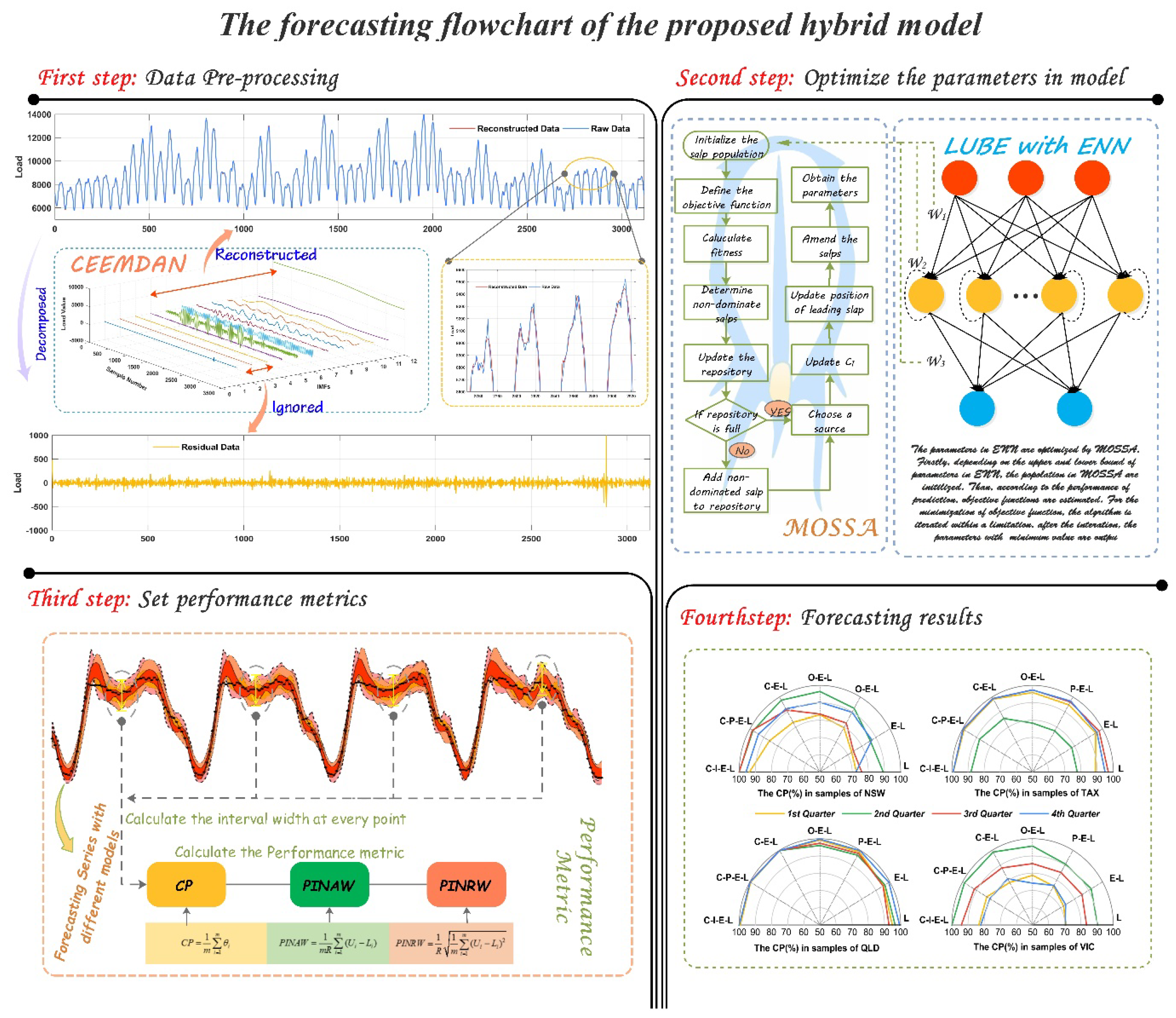
In this paper, we proposed a hybrid model for interval prediction based on the data preprocessing, multi-objective optimization algorithm and LUBE to solve the problem of STLF. This hybrid model consist of two stages: data de-noising and model prediction.

In the first stage, the main task is to refine the original data. The raw power load data is affected by many internal and external factors in the collection process. Therefore, a lot of unrelated information is integrated in the data. Several pieces of information will further affect the quality of the power load data, and increase the difficulty of accurate forecasting of the power load. In the neural network model, the performance of the model is directly affected by the quality of the data. As a type of machine learning algorithm, the neural network uses its multilayered structure to learn the relevant interdependencies of the data and determine the structural parameters of the prediction model, so as to achieve fitting and forecasting. However, if the input set of the model contains too much noise and “false information”, the model will be seriously affected in the training process, and some problems will emerge, such as the overfitting problem. Therefore, we introduced CEEMDAN to eliminate useless information in the raw data. As mentioned above, CEEMDAN can decompose the data series into several IMFs with different frequencies, as shown in Figure 2. Because the IMFs are extracted with envelope curves depending on the extremum, some of the IMFs have higher frequencies, just as the first few IMFs that are shown in Figure 2. In addition, the other IMFs also have lower frequencies and represent the trend factors, thereby formulating the vital basis for time-series prediction. In the actual operations, we can remove the IMFs with higher frequencies, which effectively represent noise to refine the original data. In order to determine which IMFs ought to be abandoned, we calculated the entropy of each IMF and removed the IMFs with lower entropy. After the denoising process, the refined data are transferred to next stage as the input data for training in the predictive model.

In the second stage, the main interval prediction model was proposed. In our hybrid interval prediction model, the PI is output dependent on LUBE, which is based on the multi-output of the Elman neural network (E–LUBE). In the training process, the input set of E–LUBE is constructed as indicated in Formula (16), while the output set is constructed as indicated in Formula (17), where m and s respectively denote the number of features and the numbers of samples, and $\alpha$ denotes the interval width coefficient. In the case of the STLF problem, m indicates the number of previous time-points that we use to forecast the predictive value.

$$\mathrm{Input}\mathrm{set}:\left[\begin{array}{cccc}{x}_1& x_2& \cdots & x_m\\ x_2& x_3& \cdots & x_{m+1}\\ ⋮& ⋮& \ddots & ⋮\\ x_s& x_{s+1}& \cdots & x_{s+m}\end{array}\right]$$

(16)

$$\mathrm{Output}\mathrm{set}:\left[\begin{array}{c}{x}_{m+1}\times (1-\alpha )\\ x_{m+2}\times (1-\alpha )\\ ⋮\\ x_{m+s+1}\times (1-\alpha )\end{array}\begin{array}{c}\\ \\ \\ \end{array}\begin{array}{c}{x}_{m+1}\\ x_{m+2}\\ ⋮\\ x_{m+s+1}\end{array}\begin{array}{c}\\ \\ \\ \end{array}\begin{array}{c}{x}_{m+1}\times (1+\alpha )\\ x_{m+2}\times (1+\alpha )\\ ⋮\\ x_{m+s+1}\times (1+\alpha )\end{array}\right]$$

(17)

According to a trained model, when a new series X_i, i = 1, …, m, is input into the model, X_m+1 with an upper bound $X_{m+1}^U$ and a lower bound $X_{m+1}^L$ will be output. This is the basic mechanism of interval prediction for STLF in this study. However, in traditional multi-output neural networks, the loss function is always the mean-square-error (MSE), which is a key criterion for point forecasting. In this study, we introduced two new criteria (PIW and CP) to construct the loss function, considering the main purpose of our interval prediction. The traditional neural network parameters were determined by using a gradient descent algorithm, but for two of the set criteria, the calculation of the gradient was difficult. Therefore, we employed MOSSA to realize the multi-objective parameter optimization. Furthermore, the optimization problem can be expressed as,

$$\begin{array}{cc}argmin& \{\begin{array}{c}\mathrm{PIW}(\theta )\\ \raisebox{1ex}{$1$}\!\left/ \!\raisebox{-1ex}{$\mathrm{CP}(\theta )$}\right.\end{array}\end{array}$$

(18)

where $\theta$ is a set of parameters in E–LUBE, including the weight and bias.

When the parameters are determined in the training process, the entire model can be applied to the test set to verify the performance of interval prediction.

4. Simulations and Analyses

In order to validate the performance of the proposed hybrid model in STLF, four electrical load datasets collected from four states in Australia are used in our research. The four states include New South Wales (NSW), Tasmania (TAX), Queensland (QLD) and Victoria (VIC), and the specific location is showed in Figure 3. The experiments in this study consist of two parts: experiment I and experiment II. For experiment I, the load data of four states are modeled with interval width coefficient $\alpha =0.05$, and for the experiment II, the interval width coefficient $\alpha$ is set as 0.025 for further analysis. In order to verify the superiority of the proposed hybrid model, several benchmark models which include basic LUBE (LUBE), LUBE with Elman neural network (E–LUBE), E–LUBE with point optimization (PO–E–LUBE), E–LUBE with interval optimization (IO–E–LUBE), and models integrated with CEEMDAN, are exhibited. For persuasive comparability and fairness, the hyper-parameters in each model are consistent, as shown in

Table 1. Related parameters in hybrid model.

Submodels and Parameters	Value
Elman Neural Network (ENN)
Inputnum	6
Hiddennum	13
Outputnum	3
Train.epoch	500
Train.lr	0.1
Train.func	“Adam”
Complete ensemble empirical mode decomposition with adaptive noise (CEEMDAN)
Nstd	0.2
NR	200
Maxiter	100
Multi-objective salp swarm algorithm (MOSSA)
Dim	754
Lb	−2
Ub	2
Obj_no	2
Pop_num	50

. All experiments have been carried out in MATLAB 2016a on a PC with the configuration of Windows 7 64-bit, Inter Core i5-4590 CPU @ 3.30GHz, 8GB RAM.

4.1. Data Descriptions

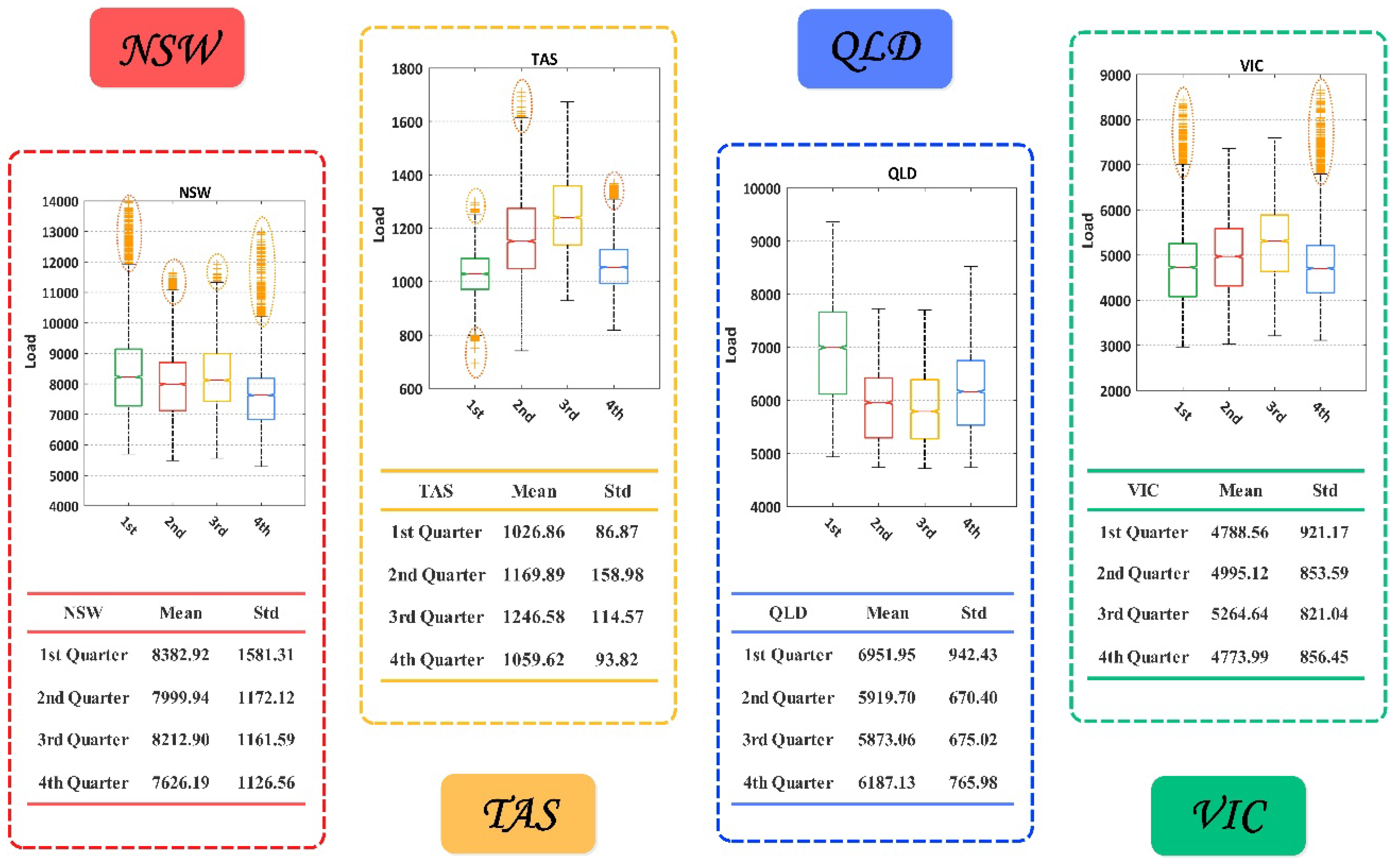
For each state, we considered the data using half an hour interval in four quarters. The data used in this paper can be obtained on the website of Australian energy market operator (http://www.aemo.com.au/). We chose data from the whole of 2017 from 1 January 2017 0:30 am to 31 December 2017 0:00 am to construct dataset. In each state, the total sample number is 17,520. For each quarter, the number of samples were 4320, 4358, 4416, 4416 respectively. In order to control the comparability, we selected 1200 samples to test the trained model, and used the rest in each quarter to train the models. The proportion of train sets versus the test sets was approximately equal to 3:1. The description of the data characteristics are shown in Figure 4. Considering the structure of the neural network in this study, we set six input neurons, 13 hidden neurons, and three output neurons. Specifically, the output set was formulated in accordance with Formula (17).

During data preprocessing, the input data were divided into several IMFs depending on CEEMDAN, as displayed in Figure 2. According to the energy entropy of each IMF shown in Figure 3, we ignored the IMFs which contained high frequencies, and summed the rest of the IMFs to reconstruct the input set, as shown in Figure 1.

4.2. Performance Metrics

In order to comprehensively assess the performance of the models, some metrics were employed. These metrics primarily focused on the coverage of the real value in the prediction interval and the width of the interval.

4.2.1. Coverage Probability

Coverage probability [50] is usually considered as a basic feature of PIs and CP is calculated according to the ratio of the number of target values covered by PIs:

$$\mathrm{CP}=\frac{1}{m}{\displaystyle \sum _{i=1}^m{\theta }_i}$$

(19)

where m denotes the number of samples, and ${\theta }_i$ is a binary index which measures whether the target value is covered by PIs:

$${\theta }_i=\{\begin{array}{c}1\begin{array}{ccc}& ,& y_i^t\in [{\widehat{L}}_i,{\widehat{U}}_i]\end{array}\\ 0\begin{array}{ccc}& ,& y_i^t\notin [{\widehat{L}}_i,{\widehat{U}}_i]\end{array}\end{array}$$

(20)

where $y_i^t$ denote the ith target value and ${\widehat{L}}_i$, ${\widehat{U}}_i$ represent the ith lower bound and the upper bound, respectively.

A larger CP means more targets are covered by the constructed PIs and a too small CP indicates the unsatisfied coverage behaviors. To have valid PIs, CP should be larger or at least equal to the nominal confidence level of PIs. Furthermore, in this paper, CP is also an important factor in the process of parameter optimization by the multi-objective optimization algorithm.

4.2.2. Prediction Interval (PI) Normalized Average width and PI Normalized Root-Mean-Square Width

In research studies on interval prediction, more attention is usually paid to CP. However, if the lower and upper bounds of the PIs are expanded from either side, any requirement for a larger CP can be satisfied, even for 100%. However, in some cases, a narrower interval width is necessary for a more precise support for electric power supply. Therefore, the width between the lower and upper bounds should be controlled so that the PIs are more convincing. In this study, the prediction interval width (PIW) is another factor in the process of parameter optimization. With CP and PIW, two objects compose the solution space within which the Pareto solution set is estimated.

In order to eliminate the impact of dimension, some relative indexes should be introduced to improve the comparability of width indicators. Inspired by the mean absolute percentage error (MAPE) in point forecasting, we employed PI normalized average width (PINAW) and PI normalized root-mean-square width (PINRW) [50]:

$$\mathrm{PINAW}=\frac{1}{mR}{\displaystyle \sum _{i=1}^m(U_i-L_i)}$$

(21)

$$\mathrm{PINRW}=\frac{1}{R}\sqrt{\frac{1}{m}{\displaystyle \sum _{i=1}^m{(U_i-L_i)}^2}}$$

(22)

where R equals to the maximum minus minimum of the target values. Normalization by the range R is able to improve comparability of PIs constructed using different methods and for different types of datasets.

4.2.3. Accumulated Width Deviation (AWD)

Accumulated width deviation (AWD) is a criterion that measure the relative deviation degree, and it can be obtained by the cumulative sum of AWD_i [55]. The calculation formula of AWD is expressed as Equations (23) and (24), where α denotes the interval width coefficient and I_i represents the i-th prediction interval.

$$AW{D}_i=\{\begin{array}{c}\frac{L_i^{(\alpha )}-z_i}{U_i^{(\alpha )}-L_i^{(\alpha )}},z_i<L_i^{(\alpha )}\\ 0,\begin{array}{ccc}& & \end{array}{z}_i\in I_i^{(\alpha )}\\ \frac{z_i-U_i^{(\alpha )}}{U_i^{(\alpha )}-L_i^{(\alpha )}},z_i>U_i^{(\alpha )}\end{array}$$

(23)

$$AW{D}^{(\alpha )}=\frac{1}{n}{\displaystyle \sum _{i=1}^{n}AW{D}_i^{\alpha }}$$

(24)

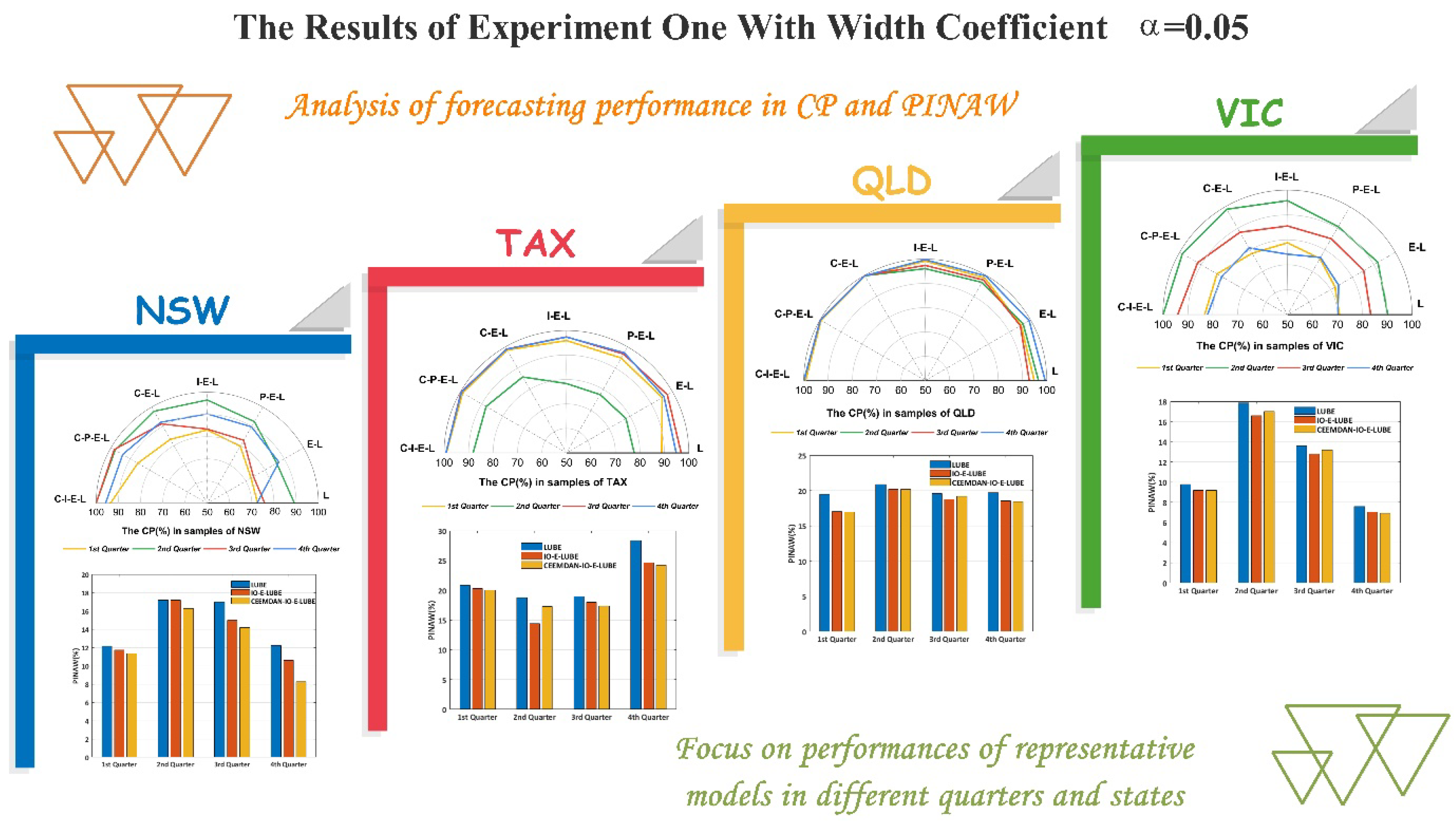
4.3. Experiment I: Cases with Larger Width Coefficients

In this experiment, we set the interval width coefficient $\alpha =0.05$, which is equivalent to setting the output to $[0.95\times X,X,1.05\times X]$ for a single sample in the training process of the neural network. Based on this structure, the PIs can be output given an input test set. In order to guarantee the diversity of the samples, we studied four different quarterly data for four different states.

The models involved in our research can be divided into three groups for better explanations for the impact of different components. The first group included LUBE and E–LUBE, and the difference between them were the structures of the neural network. The structure of LUBE consisted of three layers which were similar to the traditional BP neural network. Moreover, in the E–LUBE, an extra context layer was added to the structure so that we could validate the impact of the context layer in prediction by comparing the performance of these two models. The second group included the PO–E–LUBE and IO–E–LUBE, and the difference between them included the optimization algorithm in the training process. PO–E–LUBE used the error and variance of point prediction to construct the cost function in MOSSA, whereby the target of minimizing the cost function effectively denotes a requirement for better prediction accuracy. In addition, IO–E–LUBE employed the CP and PIW of the interval prediction to construct the cost function in multi-objective optimization, while the target of minimizing such a cost function denoted the requirements for a better performance in interval coverage, which is more rational for our goal of interval prediction. The comparison between such models can reflect the influence of different cost functions in the parameter optimization process. Furthermore, in the first group, the parameters of the neural network are determined by a conventional gradient descent algorithm, and in the second group, the parameters are determined by a heuristic optimization algorithm. Therefore, the impact of different optimization algorithms can be shown by comparing the models in different groups. In addition, in the third group, the data preprocessing is introduced. Based on the models in the first two groups, CEEMDAN was used to refine the input dataset. The results of the models in this group will display the effect of data preprocessing in the hybrid model.

The simulation results are shown in

Table 2. Results of different models with $\alpha =0.05$ for sample in New South Wales (NSW) and Tasmania (TAX).

Models	Criterion (%)
NSW	First Quarter				Second Quarter				Third Quarter				Fourth Quarter
	CP	PINAW	PINRW	AWD	CP	PINAW	PINRW	AWD	CP	PINAW	PINRW	AWD	CP	PINAW	PINRW	AWD
LUBE	72.66	12.13	12.90	0.030	89.22	17.20	18.01	0.020	75.88	16.97	17.14	0.022	72.36	12.23	13.85	0.085
E-LUBE	72.75	12.00	12.92	0.037	86.08	17.37	18.20	0.023	74.00	16.14	16.41	0.025	87.17	12.10	13.58	0.021
PO-E-LUBE	79.67	11.80	12.58	0.010	92.42	17.25	17.83	0.007	82.75	14.98	15.29	0.049	89.75	11.26	12.86	0.033
IO-E-LUBE	83.00	11.72	12.50	0.032	96.50	17.19	17.68	0.003	83.42	14.96	15.25	0.115	90.25	10.62	11.65	0.015
CEEMDAN-E-LUBE	83.25	11.67	12.36	0.021	97.83	17.10	17.90	0.002	91.25	14.75	15.28	0.007	92.08	10.48	11.23	0.022
CEEMDAN-PO-E-LUBE	86.08	11.52	12.24	0.099	97.83	16.66	17.26	0.002	98.33	14.47	14.99	0.005	93.92	10.46	10.97	0.043
CEEMDAN-IO-E-LUBE	93.58	11.36	12.24	0.016	100.00	16.27	16.66	0.000	100.00	14.18	15.72	0.000	95.75	8.28	10.26	0.007
TAX	First Quarter				Second Quarter				Third Quarter				Fourth Quarter
	CP	PINAW	PINRW	AWD	CP	PINAW	PINRW	AWD	CP	PINAW	PINRW	AWD	CP	PINAW	PINRW	AWD
LUBE	88.93	20.84	21.25	0.624	77.68	18.75	19.57	0.533	96.88	18.93	19.21	0.021	94.85	28.33	28.71	0.015
E-LUBE	94.17	20.63	21.10	0.020	78.08	17.45	18.97	0.127	97.58	18.17	18.80	0.008	96.00	25.04	25.52	0.016
PO-E-LUBE	94.75	20.12	20.63	0.009	78.50	16.55	17.61	0.136	97.67	17.94	18.45	0.011	97.25	25.13	25.48	0.007
IO-E-LUBE	95.92	20.29	20.65	0.007	78.33	14.38	15.74	0.257	97.42	17.96	18.60	0.006	97.33	24.67	24.98	0.008
CEEMDAN-E-LUBE	98.50	19.98	20.36	0.005	85.83	16.64	16.93	0.032	99.00	17.35	18.82	0.001	98.92	23.48	23.69	0.002
CEEMDAN-PO-E-LUBE	99.00	19.92	20.31	0.001	87.92	16.01	16.30	0.034	99.75	17.11	18.56	0.001	99.58	24.79	25.04	0.002
CEEMDAN-IO-E-LUBE	99.08	19.98	20.30	0.006	88.17	17.25	17.75	0.046	99.25	17.37	19.04	0.001	99.25	24.20	24.49	0.001

and

Table 3. Results of different models with $\alpha =0.05$ for sample in Queensland (QLD) and Victoria (VIC).

Models	Criterion (%)
QLD	First Quarter				Second Quarter				Third Quarter				Fourth Quarter
	CP	PINAW	PINRW	AWD	CP	PINAW	PINRW	AWD	CP	PINAW	PINRW	AWD	CP	PINAW	PINRW	AWD
LUBE	94.82	19.47	20.12	0.012	96.58	20.86	21.75	0.004	92.78	19.58	20.11	0.002	99.33	19.69	20.47	0.001
E-LUBE	95.50	17.29	18.38	0.007	96.50	20.96	21.54	0.003	95.17	19.32	19.85	0.001	99.33	19.10	19.80	0.000
PO-E-LUBE	98.83	17.58	18.42	0.001	96.67	20.57	21.07	0.003	97.83	19.07	19.54	0.001	99.75	19.38	20.24	0.001
IO-E-LUBE	99.17	17.03	17.77	0.006	96.78	20.18	21.86	0.003	97.42	18.79	19.27	0.002	99.75	18.53	19.04	0.000
CEEMDAN-E-LUBE	99.75	18.17	18.88	0.000	99.83	20.69	21.60	0.000	99.92	19.32	19.86	0.000	99.83	19.49	20.10	0.000
CEEMDAN-PO-E-LUBE	99.50	18.26	18.97	0.001	99.83	20.19	21.71	0.000	99.92	19.42	19.93	0.000	99.83	19.26	19.80	0.000
CEEMDAN-IO-E-LUBE	99.25	16.96	17.67	0.002	100.00	20.17	21.66	0.000	99.92	19.17	19.53	0.000	99.92	18.42	18.90	0.001
VIC	First Quarter				Second Quarter				Third Quarter				Fourth Quarter
	CP	PINAW	PINRW	AWD	CP	PINAW	PINRW	AWD	CP	PINAW	PINRW	AWD	CP	PINAW	PINRW	AWD
LUBE	70.85	9.77	10.62	0.042	90.25	17.85	18.37	0.351	83.42	13.61	14.29	0.013	70.22	7.58	7.90	0.018
E-LUBE	72.08	9.41	10.29	0.020	91.92	16.66	17.41	0.127	85.33	13.25	14.02	0.008	73.67	7.04	7.87	0.016
PO-E-LUBE	76.00	9.41	10.40	0.009	92.75	15.82	16.34	0.136	85.17	13.09	14.12	0.011	76.50	6.94	7.84	0.007
IO-E-LUBE	78.83	9.18	10.18	0.007	95.75	16.61	17.32	0.257	85.58	12.82	13.91	0.006	76.25	7.04	8.22	0.008
CEEMDAN-E-LUBE	78.42	9.29	10.72	0.005	98.83	15.40	16.33	0.032	88.17	12.58	13.30	0.001	80.92	7.23	8.01	0.002
CEEMDAN-PO-E-LUBE	82.67	9.22	10.43	0.001	98.75	17.12	18.12	0.034	91.67	12.70	13.57	0.001	80.50	7.07	7.93	0.002
CEEMDAN-IO-E-LUBE	83.25	9.21	10.13	0.002	99.92	17.00	18.01	0.036	94.08	13.17	13.79	0.001	82.08	6.90	7.78	0.001

. Also shown in Figure 5 are the principal indices of interval prediction, namely, CP and PINAW. Based on the conducted comparisons referred to earlier, several conclusions can be inferred:

(1)

By comparing the models in the first group, we can conclude that the E–LUBE is superior to LUBE in most cases, such as the fourth quarter in NSW and the first quarter in TAX, as shown in Table 2 and Figure 5. The CP of E–LUBE reached 87.17%, while the CP of LUBE was 72.36% for the fourth quarter in NSW. The rate of improvement was more than 15% with the maintenance of PINAW and PINRW. However, in some cases, the improvement is not remarkable, such as the fourth quarter in QLD, as shown in Table 3 and Figure 5. The performances of these two models are almost the same. In general, the performance of E–LUBE is better than LUBE, which means that E–LUBE with an extra context layer can improve the performance. In theory, the context layers are able to provide more information compared to previous outputs of hidden layers. This superiority has been proved in our experiments. However, owing to the instability of the parameters in the neural network, the improvement is not adequately remarkable in a few cases.

(2)

In terms of the optimization methods, and according to the results shown in Figure 5, and Table 2 and Table 3, the CPs of the second group (PO–E–LUBE and IO–E–LUBE) perform better than E–LUBE in most cases. E–LUBE uses the gradient descent algorithm, which is sensitive to the initialization, in order to obtain the parameters in NN. Furthermore, the models in the second group use the heuristic swarm optimization algorithm which can synthesize the initialization results using an adequate population size. Thus, the models in the second groups should have elicited better performances in theory unless the random initializations of E–LUBE are perfect. Moreover, within the second group, IO–E–LUBE has a larger CP value than PO–E–LUBE, with low levels of PINAW and PINRW. It is just the influence of the cost function that makes such a difference. The main object of the interval prediction is a larger CP value along with a narrow width. Therefore, the IO should have an advantage

(3)

Incorporation of CEEMDAN in the hybrid models is improved the performances significantly because of the denoising preprocessing. In most cases, the CPs are larger than 80% and 90%, which means more than 80% target load values are covered by the predicted intervals. Furthermore, in some cases, the CPs can reach 100%, such as the second and third quarters in NSW, and the second quarter in QLD. Such accuracy can ensure that the power supply meets the demand. Compared with the original LUBE and E–LUBE, the hybrid model we proposed (CEEMDAN–IO–E–LUBE) elicited a significant improvement in the elicited results of interval prediction.

(4)

With a larger width coefficient, the CPs of our models were almost satisfactory. The smallest CP was more than 70%, and the largest CP was able to reach 100%, which is perfect for interval prediction in STLF. However, the PINAW and PINRW were almost all larger than 10, and even reached the value of 20 in second quarter in QLD. But the proposed model still outperforms other models.

(5)

Considering the accumulated width deviation (AWD), for a larger width coefficient, the proposed model (CEEMDAN-IO-E-LUBE) has a smaller AWD compared with other benchmark models in most cases. According to the definition of AWD, a smaller AWD means more target values fall into the predicted intervals. For the results in which the target values are over the bounds, the deviations are relatively small. In this experiment, the AWDs of the proposed model are satisfactory in most case. For some cases, the AWDs is even closed to 0, which means almost all target load values fall into the predicted intervals. According to these predicted intervals, load dispatch will be more rational.

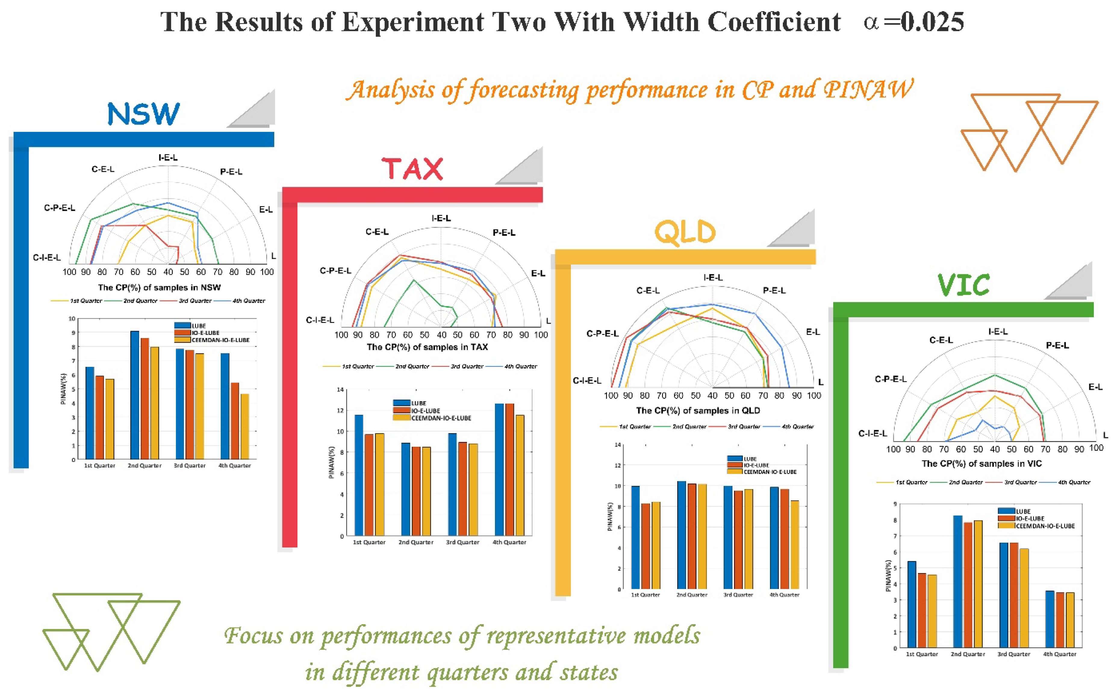
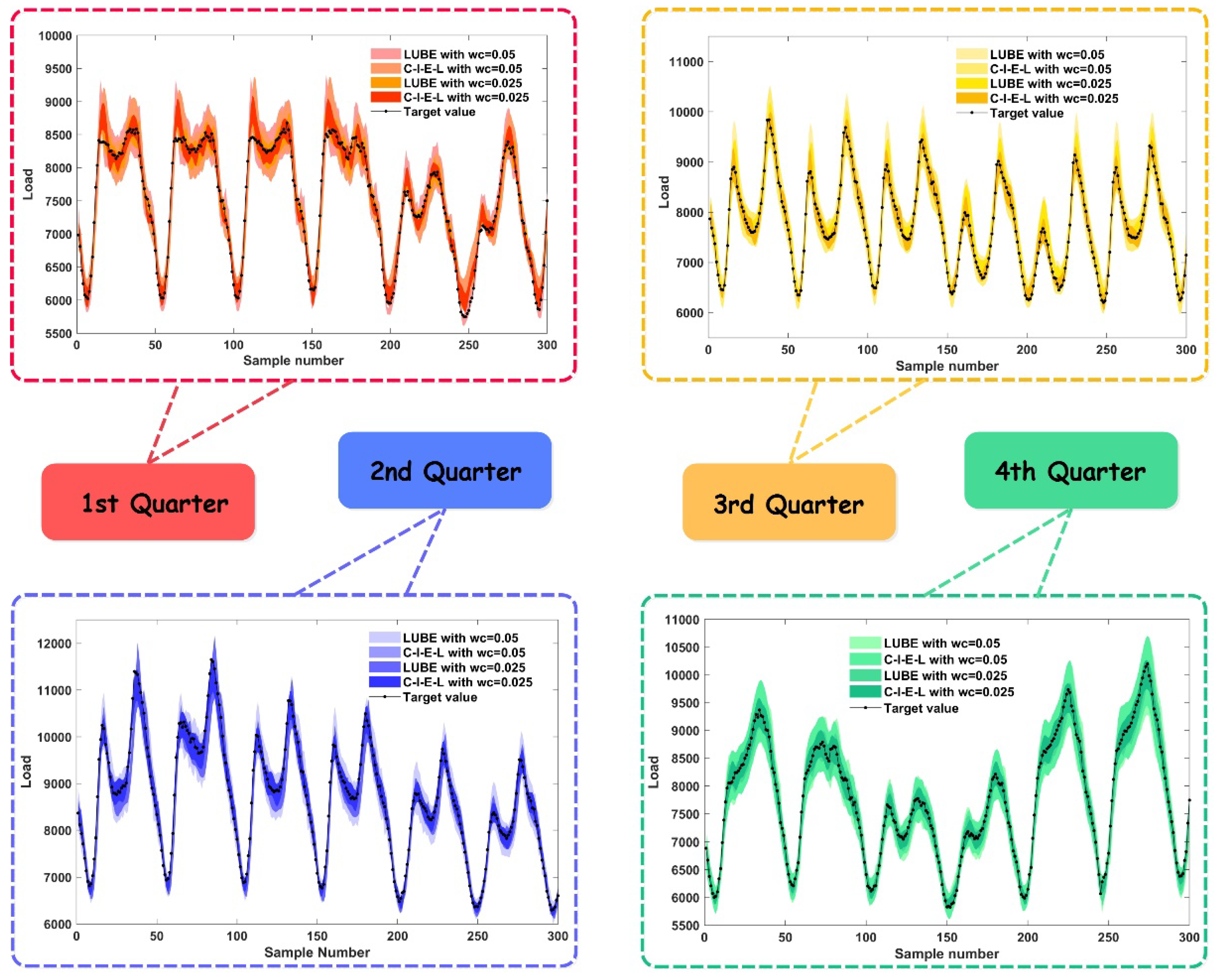
4.4. Experiment II: Cases with Smaller Width Coefficients

In this experiment, we set the interval width coefficient $\alpha =0.025$, which means we set the output to be $[0.925\times X,X,1.025\times X]$ for a single sample in the training process of the neural network. With a narrow width coefficient, the lower and upper bounds were closer to the target value in the training process, which can provide more valuable information in practice. However, a narrow bound might lead to the increase of CP. Thus, a smaller width coefficient requires the models to have better predictive properties. The results of this simulation are shown in

Table 4. Results of different models with $\alpha =0.025$ for sample in NSW and TAX.

NSW	First Quarter				Second Quarter				Third Quarter				Fourth Quarter
	CP	PINAW	PINRW	AWD	CP	PINAW	PINRW	AWD	CP	PINAW	PINRW	AWD	CP	PINAW	PINRW	AWD
LUBE	58.20	6.56	6.92	0.360	70.66	9.08	9.60	0.163	44.85	7.82	8.75	0.531	60.42	7.52	11.83	0.158
E-LUBE	58.58	5.76	6.50	0.286	70.83	9.23	9.82	0.120	46.92	7.60	8.26	0.276	60.75	7.37	12.10	0.146
PO-E-LUBE	67.50	6.00	6.51	0.061	73.67	8.41	8.79	0.027	52.33	7.82	8.64	0.515	76.08	5.66	6.60	0.126
IO-E-LUBE	67.67	5.91	6.51	0.138	73.08	8.58	8.38	0.062	51.00	7.75	8.02	0.231	77.42	5.44	6.07	0.161
CEEMDAN-E-LUBE	69.50	5.80	6.67	0.149	82.50	7.77	8.07	0.057	67.25	7.89	8.65	0.049	77.92	5.37	5.91	0.120
CEEMDAN-PO-E-LUBE	69.75	5.83	6.13	0.118	94.25	7.84	8.86	0.095	86.75	7.28	7.75	0.084	85.67	4.93	5.40	0.069
CEEMDAN-IO-E-LUBE	70.50	5.68	6.24	0.085	96.17	7.96	8.60	0.002	87.25	7.48	7.64	0.014	86.67	4.63	5.13	0.083
TAX	First Quarter				Second Quarter				Third Quarter				Fourth Quarter
	CP	PINAW	PINRW	AWD	CP	PINAW	PINRW	AWD	CP	PINAW	PINRW	AWD	CP	PINAW	PINRW	AWD
LUBE	70.61	11.52	11.83	0.187	45.78	8.84	10.80	0.534	76.87	9.78	10.85	0.126	72.31	12.61	14.04	0.120
E-LUBE	72.08	10.14	10.39	0.163	51.42	8.67	9.25	0.774	74.67	9.32	9.86	0.073	76.58	12.83	13.65	0.097
PO-E-LUBE	73.08	10.29	11.00	0.099	53.50	7.65	8.87	0.188	76.42	9.04	9.33	0.085	78.75	12.11	12.40	0.050
IO-E-LUBE	74.67	9.65	10.32	0.090	52.67	8.50	9.40	0.278	79.08	8.90	9.75	0.137	78.25	12.60	13.27	0.065
CEEMDAN-E-LUBE	88.08	10.11	10.51	0.036	72.75	9.27	9.71	0.179	90.00	8.53	8.84	0.011	86.25	11.57	11.79	0.018
CEEMDAN-PO-E-LUBE	88.08	10.04	10.24	0.019	72.00	8.57	8.82	0.194	91.50	8.60	8.89	0.009	90.75	11.56	11.84	0.013
CEEMDAN-IO-E-LUBE	88.08	9.78	10.21	0.015	74.25	8.46	8.97	0.171	93.42	8.79	8.30	0.013	91.08	11.49	11.84	0.018

and

Table 5. Results of different models with $\alpha =0.025$ for sample in QLD and VIC.

Models	Criterion (%)
QLD	First Quarter				Second Quarter				Third Quarter				Fourth Quarter
	CP	PINAW	PINRW	AWD	CP	PINAW	PINRW	AWD	CP	PINAW	PINRW	AWD	CP	PINAW	PINRW	AWD
LUBE	70.55	9.94	10.82	0.158	72.75	10.44	10.98	0.069	73.36	9.97	10.35	0.075	85.39	9.83	10.76	0.009
E-LUBE	74.75	9.29	10.00	0.024	74.42	10.13	10.43	0.065	77.58	9.57	9.87	0.058	87.17	9.77	10.01	0.008
PO-E-LUBE	80.42	8.71	9.10	0.064	78.08	10.82	11.27	0.049	80.75	9.67	9.89	0.045	90.42	10.11	10.57	0.008
IO-E-LUBE	86.83	8.26	9.71	0.309	78.33	10.16	11.61	0.072	80.50	9.50	9.75	0.046	89.17	9.66	10.11	0.003
CEEMDAN-E-LUBE	82.75	9.54	9.88	0.156	94.50	10.79	11.23	0.012	91.58	9.70	10.18	0.003	93.42	9.25	10.20	0.004
CEEMDAN-PO-E-LUBE	91.00	8.72	9.01	0.085	95.58	10.54	11.01	0.008	98.75	9.77	10.21	0.002	95.17	9.07	9.39	0.003
CEEMDAN-IO-E-LUBE	91.42	8.41	8.77	0.048	95.25	10.13	11.17	0.004	99.75	9.64	9.91	0.002	95.33	8.52	8.84	0.003
VIC	First Quarter				Second Quarter				Third Quarter				Fourth Quarter
	CP	PINAW	PINRW	AWD	CP	PINAW	PINRW	AWD	CP	PINAW	PINRW	AWD	CP	PINAW	PINRW	AWD
LUBE	50.16	5.39	6.83	0.882	70.03	8.25	8.80	0.537	68.91	6.55	7.03	0.622	50.06	3.55	4.10	0.486
E-LUBE	56.75	5.10	6.59	0.923	72.33	8.10	8.63	0.596	70.67	6.63	7.04	0.692	50.00	3.47	4.14	0.575
PO-E-LUBE	62.75	4.83	5.77	0.312	76.25	8.34	8.91	0.081	70.67	6.71	7.31	0.609	50.25	3.53	4.04	0.127
IO-E-LUBE	66.75	4.63	5.47	0.805	79.25	7.82	8.79	0.131	70.00	6.54	7.03	0.013	49.50	3.44	5.22	0.226
CEEMDAN-E-LUBE	60.00	4.75	5.28	0.433	75.83	8.04	8.31	0.059	73.42	6.64	7.04	0.038	54.50	3.68	4.45	0.262
CEEMDAN-PO-E-LUBE	65.83	4.64	5.35	0.123	83.50	8.66	9.27	0.127	78.92	6.98	7.32	0.033	53.25	4.00	4.93	0.473
CEEMDAN-IO-E-LUBE	68.25	4.56	5.64	0.081	94.08	7.93	8.23	0.044	85.75	6.18	6.70	0.043	69.33	3.44	4.45	0.161

, and in Figure 6. Correspondingly, the following conclusions can be drawn:

(1)

As Table 4 and Figure 6 show, the distinction of the models is similar to experiment I. The CPs of the original LUBE and E–LUBE are the smallest among the models in our simulation, and our proposed model CEEMDAN–IO–E–LUBE elicits the best performance

(2)

For some benchmark models in this experiment, with a narrow bound in the training process, the performance was not adequately satisfactory. As the cases of the third quarter in NSW denote and the second quarter in TAX show the CPs of LUBE and E–LUBE are close to 50%, which is not conclusive in practice. However, based on the hybrid mechanism we proposed, the performances were improved significantly. The minimum CP values of CEEMDAN–IO–E–LUBE can reach 70%, and the maximum is close to 100%, such as in the third quarter in QLD. Such results show that the predicted intervals can better cover actual electricity demand data and economize spinning reserve in power grid.

(3)

With a smaller width coefficient, the CPs decreased while the PINAW and PINRW are reduced. For the benchmark models, the results mostly display smaller CPs and larger PINAW or PINRW. However, the proposed model is able to demonstrate larger CPs with smaller PINAW and PINRW values, which is equivalent to a good performance in interval prediction. In some cases, the CP values were larger than 95% with PINAW and PINRW values less than 10. In such cases, the CPs are satisfactory and the widths of the PIs are most appropriate.

(4)

In terms of AWD in this experiment, the proposed model still showed a relatively small AWD compared with other benchmark models, which means the proposed model has a better performance at predicted accuracy. Compared with experiment I, the AWDs in this experiment are bigger. For a smaller width coefficient, the predicted interval will be narrower, which means there will be more target points falling outside the intervals. In some situations, a narrower predicted interval is necessary. The proposed model is able to provide a better performance on the condition of the requirement of a narrower predicted interval of electric load.

4.5. Comparisons and Analyses

According to the comparison of the above two experimental results, the width coefficient has a significant influence on performance, as shown in Figure 7. From one perspective, for most models, a coefficient with a larger width may lead to a larger and more satisfactory CP value, but the index about the width of PI may not be desired. From another perspective, for most models, a narrower width coefficient may elicit the desired PINAW and PINRW values, but the CP is not good enough. Considering such a situation, the proposed models alleviate the contradiction. Even though the CP value of the proposed model will decline when the width coefficient decreases, comprehensive performance is satisfactory. In some exceptional cases, owing to the complexity and instability of the datasets, the performance of the proposed models is not adequate, as the description in Figure 3 shows.

5. Discussion

In this section, we discuss some factors which may have an effect on the performances of the proposed models in order to improve the practicability of our hybrid model. The factors involved mainly include the features of the datasets and the setting of the hyperparameters in the algorithm.

5.1. Dataset Features

The feature and quality of the datasets have a significant effect on the performance of the prediction models. In STLF, the data shows periodicity and volatility. The periodicity is attributed to the regularity in the actual use of electricity, and the volatility is attributed to the randomness and occasional use of electricity. Therefore, the linear component and the non-linear components operate simultaneously during the forecasting of the model. Specifically, some outliers may have a negative effect in the process of prediction.

As Figure 4 shows, the dataset features of the different samples are various. According to the boxplot theory, the data points that are larger than Q3 + 1.5IQR or smaller than Q1 − 1.5IQR are regarded as outliers. For the first and fourth quarters in NSW, and the first and fourth quarters in VIC, the distributions of the datasets displayed a number of outliers. Additionally, the results of the models shown in Table 2, Table 3, Table 4 and Table 5 demonstrate that the model performance of the sample whose distribution is not desired may be unremarkable. These outliers are important factors that lead to such results, even if the CEEMDAN model has been applied in data preprocessing.

Another set of data features that may cause an unsatisfactory result are the non-linear characteristics of the dataset. It is well known that in traditional research, the prediction of regular and linear time series are easy to reach the desired accuracy. However, unstable and non-linear time series are more difficult to forecast in spite of the applications of novel models, such as the case of machine learning algorithms. A method used to measure the instability of data series is the recurrence plot (RP) [56]. A recurrence plot is an advanced technique of non-linear data analyses. It is the visualization (or a graph) of a square matrix in which the matrix elements correspond to those times at which the state of the dynamical system recurs. Stationary systems will deliver homogeneous recurrence plots, and unstable systems cause changes in the distribution of recurrence points in the plot, which is visible and identifiable by the brightened areas. In this study, we selected VIC as an example to verify the influence of instability. Before drawing the recurrence plot, the time delay and the dimension of the embedded matrix were determined by the C–C method. Depending on the “CRP Toolbox” released by Norbert Marwan [57], the recurrence plot of the four datasets of the different quarters in VIC is shown in Figure 8.

As the figure shows, the second and third quarters in VIC display relatively homogeneous distributions, while other quarters display isolated brightened areas. According to the theory of the recurrence plot, the instabilities of the former two samples are weaker, and the other two samples reveal stronger instabilities. Furthermore, we can conclude that the performances of the forecasting models shown in Table 5 are remarkable when the dataset is relatively stable, while the unstable dataset results in an unsatisfactory performance, which cannot be avoided.

5.2. Sensitivity Analysis

The hybrid model proposed in this study is based on the structure of the neural network shown in Figure 1. In the hybrid model, the hyperparameter is a key factor that influences the model’s performance. In most studies on machine learning, the setting of the hyperparameters always depends on trials or empirical knowledge. This is the reason why many experimental results cannot be reproduced and why a considerable amount of time and energy is spent on tuning parameters in industrial applications. At present, there is no absolute method to determine the values of all types of hyperparameters. In this study, we also mainly relied on experiences and trials to set the hyperparameters, as shown in Table 1. Among the hyperparameters, several parameters need to be highlighted.

The first one is the number of salp populations in MOSSA. In the swarm heuristic optimization algorithm, the number of swarms is usually a vital factor that needs to be considered. A larger population might provide a larger probability to reach the best individual, but exceeding the desired population may cause an increase in the complexity of the algorithm, which is related to the number of algorithmic iterations. Considering the number of parameters in our proposed model, the population numbers that ranged from 10 to 100 with a step of 10 were evaluated. As a result, we selected the number 50 as the population number (as shown in

Table 6. Sensitivity analysies results of different hyper-parameters.

Metrics	The Number of Salp Populations in MOSSA
	10	20	30	40	50	60	70	80	90	100
CP	95.21	95.32	97.01	96.66	98.69	98.33	98.50	97.85	97.46	98.10
PINAW	17.34	17.63	13.52	13.89	13.10	13.02	13.64	14.05	13.82	13.72
PINRW	18.28	18.05	14.18	14.35	13.84	13.75	14.36	14.92	14.67	14.53
Time(s)	425	452	472	524	548	593	668	734	869	10.45
Metrics	The Initial Threshold of Parameters
	[−0.5, 0.5]		[−1, 1]		[−2, 2]		[−3, 3]		[−5, 5]
CP	97.65		98.84		99.00		98.26		96.89
PINAW	14.36		12.82		12.80		13.12		13.68
PINRW	15.32		13.46		13.42		13.94		14.36
Time(s)	433		450		461		453		484

) after comprehensively considering the time complexity and model performance.

The second type of hyperparameters that need to be emphasized are the upper and lower bounds of individual parameters in MOSSA. In our simulation, the datasets were normalized within the range of −1 to 1 in order to avoid the influence of dimension and improve the training speed. Therefore, the absolute value of weights and thresholds of neural networks in the training process will not be too large. As Table 6 shows, we set the initial upper and lower bounds to 2 and −2 according to the experiment trials. Excessive range limits may increase the difficulty of searching for the best parameters with a limited number of iterations. Furthermore, the algorithm that operates based on a small range may not elicit the optimal solution.

5.3. Consistency Analysis

In this section, in order to verify the consistency of our proposed model, new datasets involving latest dates are introduced. In addition, several basic compared models including long short-term memory (LSTM) networks, function fitting neural networks (FITNET), and least squares support vector machine (LSSVM) which have been proved to provide good results for STLF are employed to verify the advantages of the proposed model.

We chose NSW and VIC randomly as examples. The new datasets are collected from 1 January 2018 0:30 am to 30 May 2018 0:00 am and the total number of samples is 7152. The samples in the second quarter in NSW and the fourth quarter in VIC are chosen as compared datasets. According to the results shown in

Table 7. Consistency analysis results of some basic models and new datasets.

Models	NSW-2018-NEW					VIC-2018-NEW
	CP	PINAW	PINRW	AWD	Time(s)	CP	PINAW	PINRW	AWD	Time(s)
Proposed	89.58	15.51	16.58	0.023	593.29	89.08	11.50	12.66	0.065	564.55
LSSVM	78.67	15.95	17.64	0.677	495.32	86.67	12.16	13.01	0.026	486.85
FITNET	72.08	16.25	17.24	0.043	405.52	74.33	11.66	12.95	0.087	300.72
LSTM	44.00	5.47	5.92	0.382	1199.04	59.83	5.28	5.79	0.250	947.78
Models	NSW-2017-2Q					VIC-2017-4Q
	CP	PINAW	PINRW	AWD	Time(s)	CP	PINAW	PINRW	AWD	Time(s)
Proposed	100.00	16.27	16.66	0.000	543.20	82.08	6.90	7.78	0.001	526.39
LSSVM	94.42	16.67	17.12	0.038	409.24	71.58	7.60	10.59	0.097	435.50
FITNET	94.33	15.83	17.29	0.012	402.12	74.33	7.88	8.94	0.076	504.31
LSTM	70.67	6.01	6.37	0.101	753.60	65.33	3.10	3.55	0.248	732.21

, the proposed model also has a good performance on the new datasets. The CP is almost 90%, which means the predicted interval can cover 90% target load value. The consistency of the proposed can be guaranteed, and the change of the dates of dataset will not risk altering the final conclusion.

Considering different basic models for STLF, we chose three widely used artificial intelligence models (LSTM, FITNET, and LSSVM) as comparators to verify the superiority. As shown in Table 7, the proposed models provide a larger CP and smaller PINAW compared with the other three models. In particular, LSTM reveals desired narrower PINAW and PINRW, but the CPs are not satisfactory. Moreover, the proposed model outperformed than other basic models in AWD. Therefore, the proposed approach have a distinct advantage in the performance of short-term power load interval forecasting. It is able to provide a satisfactory CP and restrict the interval width at the same time, which is the most important aspect of superiority of the proposed model.

On the other hand, in order to obtain a better performance and accuracy, the proposed approach is more complex. The algorithm with higher complexity often takes longer in practice. As Table 7 shows, compared with LSSVM and FITNET, the execution times of the proposed model are longer, which is the major disadvantage. However, with the development of hardware, the operational capability of computer can be improved, and the execution time can be reduced. Furthermore, as a kind of artificial intelligence technique, the fine-tuning of hyper-parameters in the proposed model will take time, which is a common situation in academic and industrial fields.

5.4. Further Research Prospect

This paper proposes a hybrid interval prediction model to predict the power load intervals. Compared with other basic models, this model has achieved good results in terms of coverage, interval width, and deviation error of the prediction interval. The model can obtain relatively high coverage under the condition of relatively narrow interval width, and the interval obtained can accurately reflect the changes of future short-term power load and provide more accurate and reliable support for power dispatch. On the other hand, for datasets with more complex changes and non-linear features, although the performance of proposed model is improved compared with the traditional models, it is still not ideal in some cases. For the unfavorable results caused by the characteristics of datasets, we may explore the following two aspects in future:

(a)

Finding and improving prediction methods that can better solve the non-linear characteristics of electrical loads, and improving the performance of predictive models in complex situations;

(b)

Fully analyzing the relevant characteristics in the power load data, selecting different models for different characteristics, and using ensemble learning to integrate and enhance the prediction results.

6. Conclusions

STLF is the basic work of power system planning and operation. However, the power load has regularity and certain randomness at the same time, which increases the difficulty of desired and reliable STLF. Moreover, compared with the prediction of specific points, interval prediction may provide more information for decision making in STLF. In this study, based on LUBE, we developed a novel hybrid model including data preprocessing, a multi-objective salp algorithm, and E–LUBE. In theory, such a hybrid model can reduce the influence of noise in a dataset and the parameter optimization process is more effective and efficient in E–LUBE.

In our proposed approach, we used a multi-objective optimization algorithm to search for the parameters of the neural network and reconstructed the cost function with double interval criterions instead of point criterions (such as MSE) in the traditional method. As Table 2, Table 3, Table 4 and Table 5 show, by comparing it with traditional methods, the proposed approach provides a higher CP and a lower interval width at the same time, which makes up for the lower CP and higher interval width of traditional methods.

In order to verify the performance of the proposed model and validate the impact of the constituent components in a hybrid model, we collected 16 samples involving four states using four quarters in Australia, and set several model comparisons in experiments

Furthermore, according to the comparison and analyses results, the conclusions are summarized as follows: (a) an efficient data preprocessing method was applied herein. Depending on the decomposition and reconstruction, this method can significantly improve the model performance in STLF. (b) Compared to the traditional prediction models based on neural networks, the newly developed E–LUBE method has an advantage in terms of comprehensive performance in interval prediction. It can be validated that the context layer with the information of the former hidden layer can improve model performance. (c) The introduction of the novel multi-objective algorithm MOSSA optimized the process of parameter search. The new cost function was based on a double-objective interval index that outperformed the traditional single-objective point error index (such as MSE) in interval prediction. (d) For STLF based on the E–LUBE mechanism, the width coefficient is an important factor. A larger width coefficient may lead to satisfactory CPs, and a smaller width coefficient may result in a satisfactory interval width. Therefore, in practice, the decision maker needs to adjust the width coefficient for specific demands. For example, we chose the width coefficient with a minimum interval width at the same time that the minimum demand of CP was guaranteed. (e) No matter how complex is the dataset, the proposed model always provides the best performance compared to benchmark models. However, because of the complexity of the data itself, some of the performance is not remarkable. In general, the proposed model provided a desired result in most cases.

Furthermore, in a power grid operator the proposed method has a strong practical application significance. A highly accurate forecasting method is one of the most important approaches used in improving power system management, especially in the power market [58]. In actual operation, for secure power grid dispatching, a control center has to make a prediction for the subsequent load. According to historical data, the dataset for the predictive model involved can be constructed. The results of the predictive model are able to provide the upper bound and lower bound of the load at some point in the future. Depending on the upper bound and lower bound, the control center can adjust the quantity of electricity on each charging line. Therefore, such a hybrid approach which can provide more accurate results can ensure the safe operation of the power grid and improve the economic efficiency of power grid operation.

References

1. Fan, S.; Hyndman, R.J. Short-term load forecasting based on a semi-parametric additive model. IEEE Trans. Power Syst. 2012, 27, 134–141. [Google Scholar] [CrossRef]
2. Du, P.; Wang, J.; Yang, W.; Niu, T. Multi-step ahead forecasting in electrical power system using a hybrid forecasting system. Renew. Energy 2018, 122, 533–550. [Google Scholar] [CrossRef]
3. Shrivastava, N.A.; Khosravi, A.; Panigrahi, B.K. Prediction Interval Estimation of Electricity Prices using PSO tuned Support Vector Machines. IEEE Trans. Ind. Inform. 2015, 11. [Google Scholar] [CrossRef]
4. Hagan, M.T.; Behr, S.M. The Time Series Approach to Short Term Load Forecasting. IEEE Trans. Power Syst. 1987, 2, 785–791. [Google Scholar] [CrossRef]
5. Papalexopoulos, A.D.; Hesterberg, T.C. A regression-based approach to short-term system load forecasting. IEEE Trans. Power Syst. 1990, 5, 1535–1547. [Google Scholar] [CrossRef]
6. Christiaanse, W.R. Short-Term Load Forecasting Using General Exponential Smoothing. IEEE Trans. Power Appar. Syst. 1971, PAS-90, 900–911. [Google Scholar] [CrossRef]
7. Al-Hamadi, H.M.; Soliman, S.A. Short-term electric load forecasting based on Kalman filtering algorithm with moving window weather and load model. Electr. Power Syst. Res. 2004, 68, 47–59. [Google Scholar] [CrossRef]
8. Metaxiotis, K.; Kagiannas, A.; Askounis, D.; Psarras, J. Artificial intelligence in short term electric load forecasting: A state-of-the-art survey for the researcher. Energy Convers. Manag. 2003, 44, 1525–1534. [Google Scholar] [CrossRef]
9. Yoo, H.; Pimmel, R.L. Short term load forecasting using a self-supervised adaptive neural network. IEEE Trans. Power Syst. 1999, 14, 779–784. [Google Scholar] [CrossRef]
10. Ho, K.L.; Hsu, Y.Y.; Chen, C.F.; Lee, T.E.; Liang, C.C.; Lai, T.S.; Chen, K.K. Short term load forecasting of taiwan power system using a knowledge-based expert system. IEEE Trans. Power Syst. 1990, 5, 1214–1221. [Google Scholar] [CrossRef]
11. Mohandes, M. Support vector machines for short-term electrical load forecasting. Int. J. Energy Res. 2002, 26, 335–345. [Google Scholar] [CrossRef]
12. Hong, W.C. Electric load forecasting by seasonal recurrent SVR (support vector regression) with chaotic artificial bee colony algorithm. Energy 2011, 36, 5568–5578. [Google Scholar] [CrossRef]
13. Liu, Z.; Li, W.; Sun, W. A novel method of short-term load forecasting based on multiwavelet transform and multiple neural networks. Neural Comput. Appl. 2013, 22, 271–277. [Google Scholar] [CrossRef]
14. Fan, G.F.; Peng, L.L.; Hong, W.C.; Sun, F. Electric load forecasting by the SVR model with differential empirical mode decomposition and auto regression. Neurocomputing 2016, 173, 958–970. [Google Scholar] [CrossRef]
15. AlRashidi, M.R.; EL-Naggar, K.M. Long term electric load forecasting based on particle swarm optimization. Appl. Energy 2010, 87, 320–326. [Google Scholar] [CrossRef]
16. Wang, J.; Li, L.; Niu, D.; Tan, Z. An annual load forecasting model based on support vector regression with differential evolution algorithm. Appl. Energy 2012, 94, 65–70. [Google Scholar] [CrossRef]
17. Ghayekhloo, M.; Menhaj, M.B.; Ghofrani, M. A hybrid short-term load forecasting with a new data preprocessing framework. Electr. Power Syst. Res. 2015, 119, 138–148. [Google Scholar] [CrossRef]
18. Zhang, X.; Wang, J. A novel decomposition-ensemble model for forecasting short-term load-time series with multiple seasonal patterns. Appl. Soft Comput. J. 2018, 65, 478–494. [Google Scholar] [CrossRef]
19. Tian, C.; Hao, Y. A Novel Nonlinear Combined Forecasting System for Short-Term Load Forecasting. Energies 2018, 11, 714. [Google Scholar]
20. Khotanzad, A.; Hwang, R.C.; Abaye, A.; Maratukulam, D. An Adaptive Modular Artificial Neural Network Hourly Load Forecaster and its Implementation at Electric Utilities. IEEE Trans. Power Syst. 1995, 10, 1716–1722. [Google Scholar] [CrossRef]
21. Bishop, C.M. Neural networks for pattern recognition. J. Am. Stat. Assoc. 1995, 92, 482. [Google Scholar] [CrossRef]
22. Hwang, J.T.G.; Ding, A.A. Prediction Intervals for Artificial Neural Networks. J. Am. Stat. Assoc. 1997, 92, 748–757. [Google Scholar] [CrossRef]
23. Heskes, T. Practical confidence and prediction intervals. Adv. Neural Inf. Process. Syst. 1997, 9, 176–182. [Google Scholar]
24. Nix, D.A.; Weigend, A.S. Estimating the mean and variance of the target probability distribution. In Proceedings of the 1994 IEEE International Conference on Neural Networks (ICNN’94), Orlando, FL, USA, 28 June–2 July 1994; Volume 1, pp. 55–60. [Google Scholar]
25. Van Hinsbergen, C.P.I.; van Lint, J.W.C.; van Zuylen, H.J. Bayesian committee of neural networks to predict travel times with confidence intervals. Transp. Res. Part C Emerg. Technol. 2009, 17, 498–509. [Google Scholar] [CrossRef]
26. Khosravi, A.; Nahavandi, S.; Creighton, D. Construction of optimal prediction intervals for load forecasting problems. IEEE Trans. Power Syst. 2010, 25, 1496–1503. [Google Scholar] [CrossRef]
27. Da Silva, A.P.A.; Moulin, L.S. Confidence intervals for neural network based short-term load forecasting. IEEE Trans. Power Syst. 2000, 15, 1191–1196. [Google Scholar] [CrossRef]
28. Khosravi, A.; Nahavandi, S.; Creighton, D.; Atiya, A.F. Lower upper bound estimation method for construction of neural network-based prediction intervals. IEEE Trans. Neural Netw. 2011, 22, 337–346. [Google Scholar] [CrossRef] [PubMed]
29. Deb, K.; Agrawal, S.; Pratap, A.; Meyarivan, T. A fast elitist non-dominated sorting genetic algorithm for multi-objective optimization: NSGA-II. Parallel Probl. Solving Nat. PPSN VI 2000, 849–858. [Google Scholar] [CrossRef]
30. Deb, K.; Pratap, A.; Agarwal, S.; Meyarivan, T. A fast and elitist multiobjective genetic algorithm: NSGA-II. IEEE Trans. Evol. Comput. 2002, 6, 182–197. [Google Scholar] [CrossRef] [Green Version]
31. Coello Coello, C.A.; Lechuga, M.S. MOPSO: A proposal for multiple objective particle swarm optimization. In Proceedings of the 2002 Congress on Evolutionary Computation, CEC 2002, Honolulu, HI, USA, 12–17 May 2002; Volume 2, pp. 1051–1056. [Google Scholar]
32. Padhye, N. Topology Optimization of Compliant Mechanism Using Multi-objective Particle Swarm Optimization. In Proceedings of the 10th Annual Conference Companion on Genetic and Evolutionary Computation, Atlanta, GA, USA, 12–16 July 2008; pp. 1831–1834. [Google Scholar]
33. Alaya, I.; Solnon, C.; Ghedira, K. Ant Colony Optimization for Multi-Objective Optimization Problems. In Proceedings of the 19th IEEE International Conference on Tools with Artificial Intelligence (ICTAI 2007), Patras, Greece, 29–31 October 2007; pp. 450–457. [Google Scholar] [CrossRef]
34. Xue, F.; Sanderson, A.C.; Graves, R.J. Pareto-based multi-objective differential evolution. In Proceedings of the 2003 Congress on Evolutionary Computation, Canberra, Australia, 8–12 December 2003; Volume 2, pp. 862–869. [Google Scholar]
35. Mirjalili, S.Z.; Mirjalili, S.; Saremi, S.; Faris, H.; Aljarah, I. Grasshopper optimization algorithm for multi-objective optimization problems. Appl. Intell. 2017. [Google Scholar] [CrossRef]
36. Knowles, J.D.; Corne, D.W. Approximating the Nondominated Front Using the Pareto Archived Evolution Strategy. Evol. Comput. 2000, 8, 149–172. [Google Scholar] [CrossRef] [PubMed] [Green Version]
37. Wang, J.; Yang, W.; Du, P.; Niu, T. A novel hybrid forecasting system of wind speed based on a newly developed multi-objective sine cosine algorithm. Energy Convers. Manag. 2018, 163, 134–150. [Google Scholar] [CrossRef]
38. Du, P.; Wang, J.; Guo, Z.; Yang, W. Research and application of a novel hybrid forecasting system based on multi-objective optimization for wind speed forecasting. Energy Convers. Manag. 2017, 150, 90–107. [Google Scholar] [CrossRef]
39. Wolpert, D.H.; Macready, W.G. No free lunch theorems for optimization. IEEE Trans. Evol. Comput. 1997, 1, 67–82. [Google Scholar] [CrossRef] [Green Version]
40. Service, T.C. A No Free Lunch theorem for multi-objective optimization. Inf. Process. Lett. 2010, 110, 917–923. [Google Scholar] [CrossRef]
41. Rodriguez, P.; Wiles, J.; Elman, J.L. A Recurrent Neural Network that Learns to Count. Conn. Sci. 1999, 11, 5–40. [Google Scholar] [CrossRef] [Green Version]
42. Chandra, R.; Zhang, M. Cooperative coevolution of Elman recurrent neural networks for chaotic time series prediction. Neurocomputing 2012, 86, 116–123. [Google Scholar] [CrossRef]
43. Cacciola, M.; Megali, G.; Pellicanó, D.; Morabito, F.C. Elman neural networks for characterizing voids in welded strips: A study. Neural Comput. Appl. 2012, 21, 869–875. [Google Scholar] [CrossRef]
44. Wang, J.J.; Zhang, W.; Li, Y.; Wang, J.J.; Dang, Z. Forecasting wind speed using empirical mode decomposition and Elman neural network. Appl. Soft Comput. 2014, 23, 452–459. [Google Scholar] [CrossRef]
45. Huang, N.; Shen, Z.; Long, S.; Wu, M.; Shih, H.; Zheng, Q.; Yen, N.; Tung, C.; Liu, H. The empirical mode decomposition and the Hilbert spectrum for nonlinear and non-stationary time series analysis. Proc. R. Soc. A Math. Phys. Eng. Sci. 1998, 454, 903–995. [Google Scholar] [CrossRef]
46. Wu, Z.; Huang, N.E. Ensemble Empirical Mode Decomposition: A Noise-Assisted Data Analysis Method. Adv. Adapt. Data Anal. 2009, 1, 1–41. [Google Scholar] [CrossRef]
47. Yeh, J.R.; Shieh, J.S.; Huang, N.E. Complementary ensemble empirical mode decomposition: A novel noise enhanced data analysis method. Adv. Adapt. Data Anal. 2010, 2, 135–156. [Google Scholar] [CrossRef]
48. Torres, M.E.; Colominas, M.A.; Schlotthauer, G.; Flandrin, P. A complete ensemble empirical mode decomposition with adaptive noise. In Proceedings of the 2011 IEEE International Conference on Acoustics, Speech and Signal Processing, Prague, Czech Republic, 22–27 May 2011; Volume 7, pp. 4144–4147. [Google Scholar] [CrossRef]
49. Elman, J.L. Finding structure in time. Cogn. Sci. 1990, 14, 179–211. [Google Scholar] [CrossRef]
50. Quan, H.; Srinivasan, D.; Khosravi, A. Uncertainty handling using neural network-based prediction intervals for electrical load forecasting. Energy 2014, 73, 916–925. [Google Scholar] [CrossRef]
51. Coello Coello, C.A. Evolutionary multi-objective optimization: Some current research trends and topics that remain to be explored. Front. Comput. Sci. China 2009, 3, 18–30. [Google Scholar] [CrossRef]
52. Branke, J.; Kaußler, T.; Schmeck, H. Guidance in evolutionary multi-objective optimization. Adv. Eng. Softw. 2001, 32, 499–507. [Google Scholar] [CrossRef] [Green Version]
53. Deb, K. Advances in Evolutionary Multi-objective Optimization. In Search Based Software Engineering; Springer: Berlin/Heidelberg, Germany, 2012; pp. 1–26. ISBN 978-3-642-33119-0. [Google Scholar]
54. Mirjalili, S.; Gandomi, A.H.; Mirjalili, S.Z.; Saremi, S.; Faris, H.; Mirjalili, S.M. Salp Swarm Algorithm: A bio-inspired optimizer for engineering design problems. Adv. Eng. Softw. 2017, 114, 163–191. [Google Scholar] [CrossRef]
55. Wang, J.; Niu, T.; Lu, H.; Guo, Z.; Yang, W.; Du, P. An analysis-forecast system for uncertainty modeling of wind speed: A case study of large-scale wind farms. Appl. Energy 2018, 211, 492–512. [Google Scholar] [CrossRef]
56. Eckmann, J.-P.; Kamphorst, S.O.; Ruelle, D. Recurrence Plots of Dynamical Systems. Europhys. Lett. 1987, 4, 973–977. [Google Scholar] [CrossRef]
57. Marwan, N.; Wessel, N.; Meyerfeldt, U.; Schirdewan, A.; Kurths, J. Recurrence-plot-based measures of complexity and their application to heart-rate-variability data. Phys. Rev. E Stat. Phys. Plasmas Fluids Relat. Interdiscip. Top. 2002, 66. [Google Scholar] [CrossRef] [PubMed] [Green Version]
58. Shu, F.; Luonan, C. Short-term load forecasting based on an adaptive hybrid method. IEEE Trans. Power Syst. 2006, 21, 392–401. [Google Scholar]
Figure 1. The structure of the lower bound and upper bound estimation (LUBE) based on the Elman neural network.
Energies 11 01561 g001
Figure 2. Forecasting flowchart of the proposed hybrid model.
Energies 11 01561 g002
Figure 3. Data description of experiments. (a) Location of sample sites; (b) Division of train set and test set; (c) Structure of input set and output set; and (d) Entropy of each IMF).
Energies 11 01561 g003
Figure 4. Boxplot of the entire set of data samples.
Energies 11 01561 g004
Figure 5. Performance of different samples with the width coefficient 0.05.
Energies 11 01561 g005
Figure 6. Performance of different samples with the width coefficient 0.025.
Energies 11 01561 g006
Figure 7. Interval prediction plot of partial samples in NSW.
Energies 11 01561 g007
Figure 8. Recurrence plot of the samples obtained from the four quarters in VIC.
Energies 11 01561 g008aEnergies 11 01561 g008b