A Method for Load Classification and Energy Scheduling Optimization to Improve Load Reliability

Abstract

With the large amount of distributed generation in use, the structure of the distribution system is increasingly complex. Therefore, it is necessary to establish a method to improve load reliability. Based on the reliability model of distributed generation, this paper investigates the time sequential simulation of a wind/solar/storage combined power supply system under off-grid operation. After classifying the load by power supply region, the load weight coefficient is established, which modifies the reliability index of the load point and system. The modified expected energy not supplied (EENS) is adopted as the objective function, and the particle swarm optimization algorithm is used to solving the optimal energy scheduling for improving the load reliability. Finally, the load reliability is calculated with a hybrid method. Using the IEEE-RBTS Bus 6 system as an example, the correctness and validity of the proposed method are verified as an effective way to improve load reliability.

1. Introduction

In recent years, with the large amount of distributed generations (DGs) access, the traditional single-source radial distribution network has been transformed into a multi-source distribution system. When the system fails, a certain amount of load can be separated from the power grid to form a power supply region off-grid. In the power supply region off-grid, DGs can be used to power the load to improve reliability for users [1,2,3].

With the distribution network structure and operation mode changing, the reliability calculation method has also been changed. Many scholars have done the relevant research for the reliability evaluation of distribution networks containing DGs. In [4], a method was proposed to assess the reliability of a power distribution network with DG and a battery swapping station (BSS). The IEEE three-feeder distribution system was used to verify the effectiveness of the method. The literature [5] proposed an analytical formulation for assessing the reliability impact of energy storage supporting DG in supply restoration of isolated network areas.

The access of DGs improves the load reliability in distribution network. Literature [6] proposed a hybrid approach that combines scenario selection and enumerative analysis. The test system simulation was used to illustrate the dependence of reliability on factors. Some recommendations on the parameter settings of a protection system were provided to enhance the system reliability. In [7], the sequential Monte Carlo method was applied to complete the reliability evaluation of the RBTS Bus 4 test system. The effects on the system reliability of battery storage (BS) capacity and vehicle-to-grid (V2G) technology, driving behavior, recharging mode, and penetration of electric vehicles (EVs) were all investigated. Literature [8] proposed a constrained stochastic framework to maximize the expected profit of a microgrid operator. According to the proposed method, the impact of consumer participation demand response (DR) on system reliability is analyzed by using the conditional value-at-risk (CVaR) method. In [9], an intelligent particle swarm optimization (PSO) based search method is proposed. The reliability of the Institute of Electrical and Electronics Engineers reliability test system (IEEE RTS) was calculated by using the PSO search method.

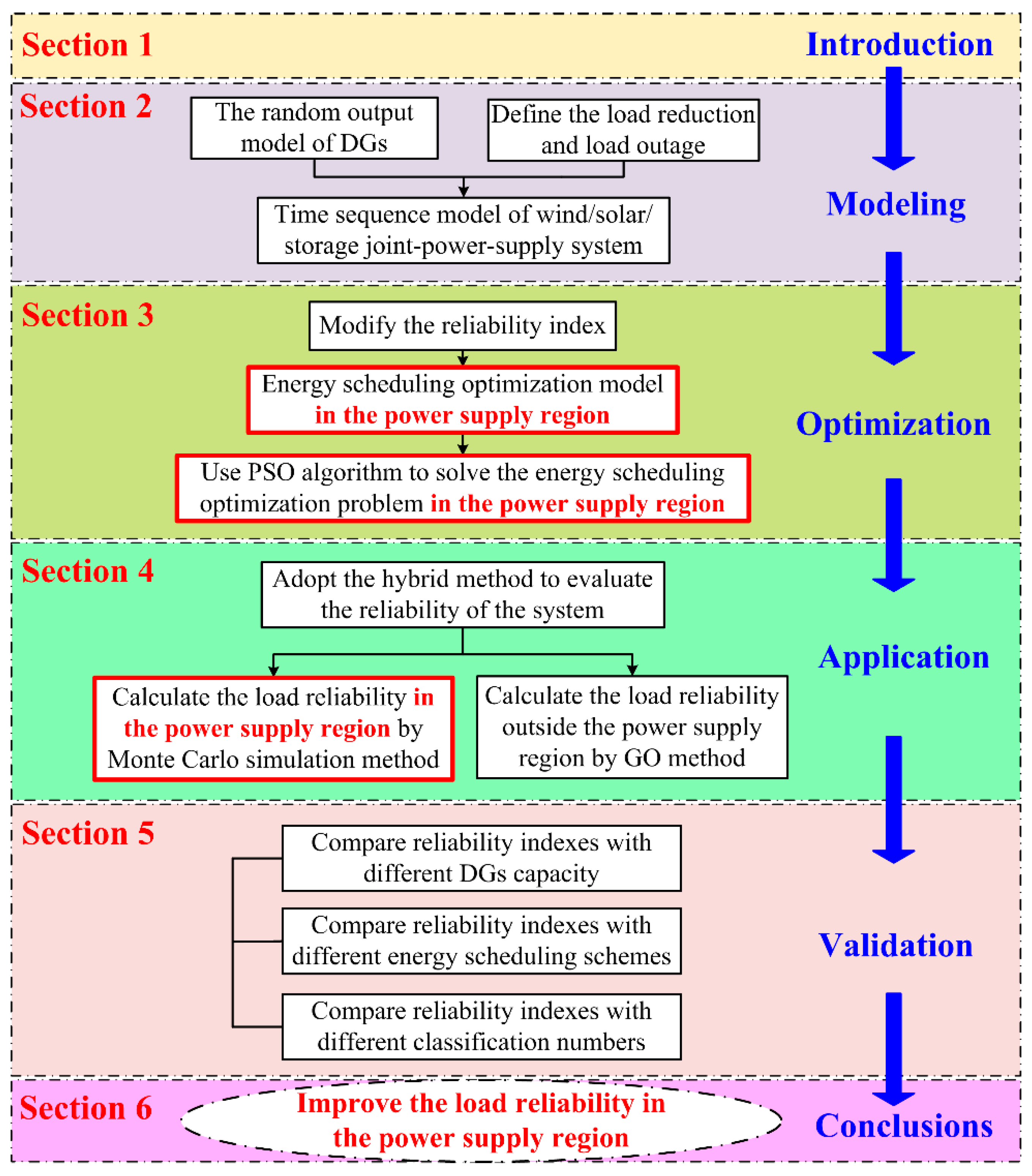
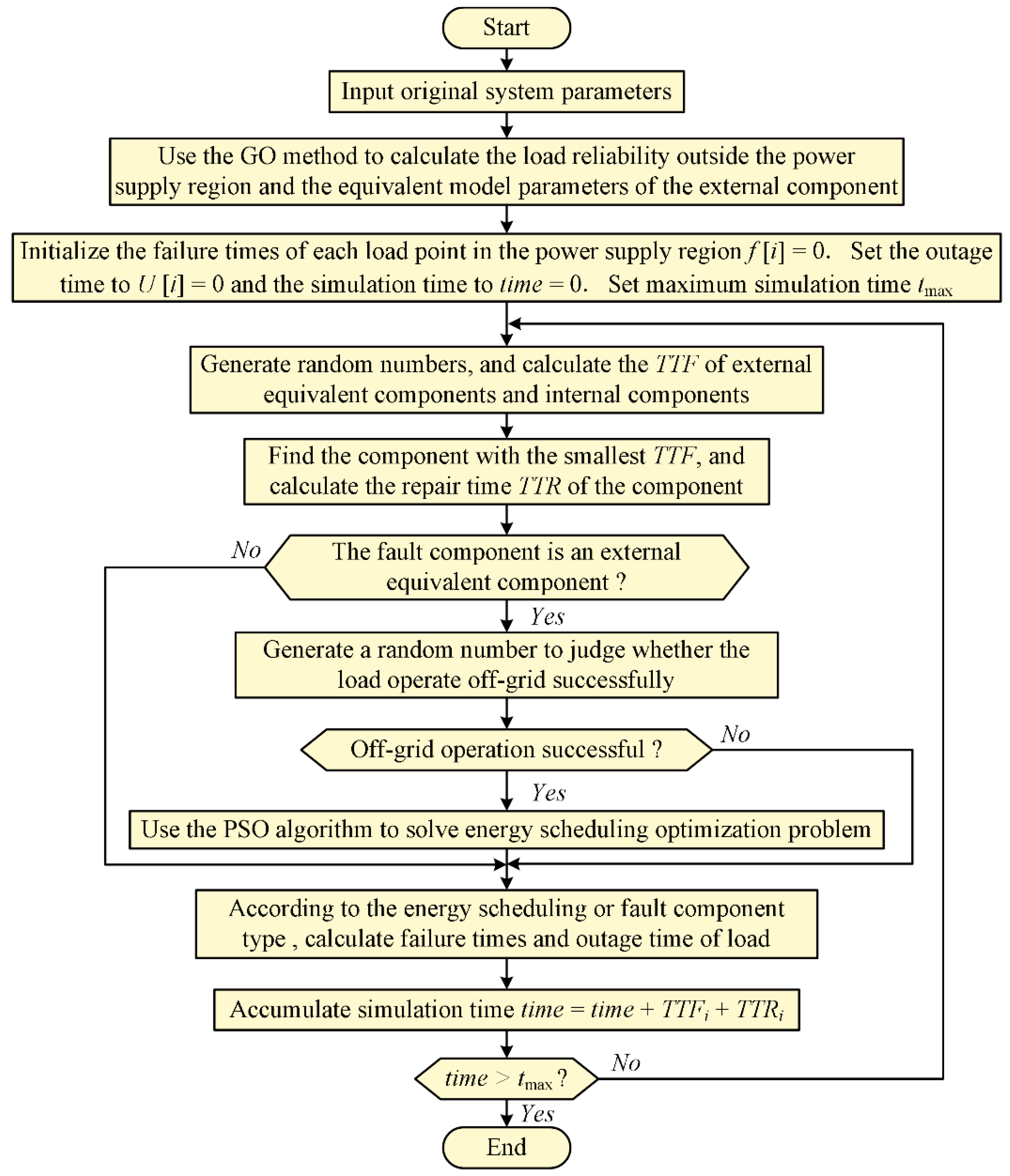
Nevertheless, there are few researches on how to improve the load reliability through the energy scheduling optimization. According to the importance of the load, the objective function of the energy scheduling optimization model in the power supply region is established in this paper. With the PSO algorithm, it obtains the optimal energy scheduling scheme. According to the optimal energy scheduling scheme, the load reliability in the power supply region is improved. The structure flow chart of this paper is shown in Figure 1.

As shown in Figure 1, the aim of this paper is to improve the load reliability in the power supply region by the energy scheduling optimization. The step-by-step description is as follows:

Section 1: The main work and contributions of this paper are introduced.

Section 2: This section researches the reliability models of DGs. After considering the random output characteristics of DGs, the timing sequence model of wind/solar/storage joint-power-supply is established.

Section 3: Considering the load weight coefficient, the reliability indexes of load point and system are modified. According to the importance of the load, the objective function of the energy scheduling optimization model in the power supply region is established. With the PSO algorithm, the optimal energy scheduling scheme is obtained.

Section 4: The load reliability is calculated by the hybrid method. The reliability of load outside the power supply region and point of common coupling (PCC) are calculated by the Goal Oriented (GO) method, and the reliability of load in the power supply region is calculated by Monte Carlo (MC) simulation. During MC simulation in the power supply region, the load classification and energy scheduling optimization in Section 3 is adopted to improve the load reliability.

Section 5: With the example system, this section verifies that the energy scheduling strategy can effectively improve the load reliability in the power supply region under the different DGs capacity, energy scheduling schemes, and the load classification numbers.

Section 6: The results of the calculation are summarized.

The primary contributions of the paper are as follows:

(1)

After considering the random output characteristics of DGs, the timing sequence model of wind/solar/storage joint-power-supply is established.

(2)

According to the load reduction and load weight coefficient, the reliability indexes of load point and system are modified. The objective function of energy scheduling optimization model in the power supply region is established. With the PSO algorithm, the optimal energy scheduling scheme is obtained.

(3)

The reliability of load is calculated by the hybrid method. With the load classification and energy scheduling optimization, the load reliability is improved.

2. Reliability Model of Distributed Generations

2.1. Wind Turbine Output Power Model

Weibull distribution is used to describe the probability distribution characteristics of the wind speed in this paper [10]. The probability density function is as follows:

$$f(v)=\frac{k}{c}(\frac{v}{c}){}^{k-1}\exp (-(\frac{v}{c}){}^k)$$

(1)

where $v$ is the wind speed, $c$ and $k$ are the scale and shape parameters, respectively.

The power output of the wind turbine (WT) depends on the wind speed. The relationship between output $P_{\mathrm{w}}(v)$ and wind speed $v$ of the wind turbine is represented as follows:

$$P_{\mathrm{w}}(v)=\{\begin{array}{l}0,v\le v_{\mathrm{ci}} \mathrm{or} v>v_{\mathrm{co}}\\ P_{\mathrm{r}}\frac{v-v_{\mathrm{ci}}}{v_{\mathrm{r}}-v_{\mathrm{ci}}},v_{\mathrm{ci}}<v\le v_{\mathrm{r}}\\ P_{\mathrm{r}},v_{\mathrm{r}}<v\le v_{\mathrm{co}}\end{array}$$

(2)

where $v_{\mathrm{ci}}$ is the cut-in wind speed, $v_{\mathrm{co}}$ is the cut-out wind speed, $v_{\mathrm{r}}$ is the rated wind speed, and $P_{\mathrm{r}}$ is the WT rated output power.

2.2. Photovoltaic Output Power Model

Solar irradiance obeys Beta distribution over a certain time period [11,12]. The probability density function is as follows:

$$f(r)=\frac{\Gamma (\alpha +\beta )}{\Gamma (\alpha )\Gamma (\beta )}(\frac{r}{r_{\max }}){}^{\alpha -1}(1-\frac{r}{r_{\max }}){}^{\beta -1}$$

(3)

where $\alpha$ and $\beta$ are the shape coefficients of Beta distribution, $\Gamma$ is the gamma function, $r$ and $r_{\max }$ are the actual light intensity and the maximum light intensity in the time period, respectively.

For a photovoltaic (PV) power generation module, the total area and the total photoelectric conversion efficiency of the battery assembly are A and $\eta$, respectively. Then the battery assembly output power is $P_{\mathrm{p}}=rA\eta$, and the output power probability density function of the PV is as follows:

$$f(P_{\mathrm{p}})=\frac{\Gamma (\alpha +\beta )}{\Gamma (\alpha )\Gamma (\beta )}(\frac{P_{\mathrm{p}}}{R_{\mathrm{p}}}){}^{\alpha -1}(1-\frac{P_{\mathrm{p}}}{R_{\mathrm{p}}}){}^{\beta -1}$$

(4)

where $R_{\mathrm{p}}=A\eta r_{\max }$ is the maximum output power of the PV generator.

2.3. Energy Storage System Model

An energy storage system can be used to smooth the random output of DGs. When the grid fails, the load in the power supply region is powered by the DGs and the energy storage system [13,14,15]. During the load off-grid operation, the energy storage system is charged when the total power output of the WT generation and the PV unit is greater than the total energy consumed by the load. The energy storage system is discharged when the total power output of the WT generation and the PV unit is less than total power of the load.

Considering the constraints of charging and discharging power and capacity of energy storage system, the model of energy storage system is established as follows:

$$\{\begin{array}{l}{P}_{\mathrm{in}}(t)\le P_{\mathrm{ch}-\max }\\ P_{\mathrm{out}}(t)\le P_{\mathrm{dch}-\max }\end{array}$$

(5)

$$\{\begin{array}{ll}{P}_{\mathrm{in}}(t)={\eta }_{\mathrm{c}}(P_{\mathrm{PV}}(t)+P_{\mathrm{WT}}(t)-P_{\mathrm{L}}(t)),& P_{\mathrm{L}}(t)<P_{\mathrm{PV}}(t)+P_{\mathrm{WT}}(t)\\ P_{\mathrm{out}}(t)=\frac{1}{{\eta }_{\mathrm{d}}}(P_{\mathrm{L}}(t)-P_{\mathrm{PV}}(t)-P_{\mathrm{WT}}(t)),& P_{\mathrm{L}}(t)\ge P_{\mathrm{PV}}(t)+P_{\mathrm{WT}}(t)\end{array}$$

(6)

$$E_{\min }\le E_{\mathrm{remain}}(t)\le E_{\max }$$

(7)

where $P_{\mathrm{in}}$ and $P_{\mathrm{out}}$ are the charge and discharge power of energy storage, $P_{\mathrm{ch}-\max }$ and $P_{\mathrm{dch}-\max }$ are the maximum charging and discharging power of energy storage system, ${\eta }_{\mathrm{c}}$ and ${\eta }_{\mathrm{d}}$ are the charge and discharge efficiency of energy storage, respectively, $E_{\mathrm{remain}}(t)$ is the remaining energy storage capacity at time $t$, $P_{\mathrm{PV}}(t)$, $P_{\mathrm{WT}}(t)$, and $P_{\mathrm{L}}(t)$ are the power of the WT generation, PV unit and load at time $t$, $E_{\max }$ and $E_{\min }$ are the maximum capacity and the minimum capacity of energy storage, respectively.

2.4. Timing Sequence Simulation of Wind/Solar/Storage Joint-Power-Supply in Off-Grid Operation

A time sequential model of wind/solar/storage is established in this paper. With the time sequential simulation method, it takes one hour as the basic step length. When the load is in off-grid operation, load reduction and load outage represent the power supply reducing and the power supply stopping to the load, respectively. It defines the power supply degree $k_i(t)$, in which $k_i(t)$ represents the ratio of the load i power consumption after and before the load reduction. When the power supply to the load is too low, the load cannot maintain the basic operation. It defines the minimum of power supply degree $k_{\mathrm{pt},i}(t)$. When the $k_{\mathrm{pt},i}(t)$ is less than $k_i(t)$, the load $i$ will be outage.

Figure 2 shows the time sequence simulation diagram of the wind/solar/storage joint-power-supply system. The abscissa represents the duration of off-grid operation; the ordinate represents the state of the load or energy storage; “1”, “0” and “−1” of the load represent the operation, outage and excessive reduce respectively; and “1” and “0” of the energy storage represent operation and outage, respectively.

As shown in Figure 2, the load can continue to operate off-grid only when the load and energy storage are in state “1”. The others cases will cause a load outage. After the fault components of the distribution network are repaired, the load can be switched to grid-connected operation.

3. Load Classification and Energy Scheduling Optimization

In this paper, the reliability indexes of load point and system are modified. According to the modified reliability index, the energy scheduling optimization model is established. With the PSO algorithm, the energy scheduling optimization problem is solved. The MC simulation method is used to simulate the power supply region off-grid operation. According to the simulation results, the energy scheduling scheme is modified again. Finally, the optimal energy scheduling scheme is obtained.

3.1. Modification of the Load and System Reliability Index

3.1.1. Modification of the Load Reliability Index Considering Load Curtailment

The power grid companies usually make compensation to users who implement load reduction or load outage by signing agreements with users [16]. In the t-th hour, the user compensation amount $C(t)$ depends on the power supply degree $k(t)$, and the relationship between the two is shown in Figure 3.

In Figure 3, $C_{\mathrm{c}}(t)$ is the user maximum compensation amount, and $k_0(t)$ is the load threshold at the t-th hour. The calculation method can effectively ensure that the user can obtain a reasonable amount of compensation after implementing load reduction or load outage, and an upper limit is set on the compensation amount at the same time.

According to the relationship between the load reduction of users and compensation amount, the reliability indexes of the load point are modified. The commonly used load point reliability indexes are failure frequency $\lambda$ and outage time $U$. Only the outage time index of the load changes with the load power supply degree. When load reduction is considered, the power outage time of load $i$ is defined as

$$\mathsf{\Delta }{U}_i(t)=\{\begin{array}{ll}{a}_i{k}_i\left(t\right)+1-a_i{k}_{\mathrm{pt},i}\left(t\right),& k_{\mathrm{pt},i}\left(t\right)\le k_i\left(t\right)\le 1\\ 1,& 0\le k_i\left(t\right)<k_{\mathrm{pt},i}\end{array}$$

(8)

$$\mathsf{\Delta }{U}_i={\displaystyle \sum _{t=1}^{T_{\max }}\mathsf{\Delta }{U}_i\left(t\right)}$$

(9)

where $\mathsf{\Delta }{U}_i(t)$ represents the equivalent outage time of load $i$ in the t-th hour, $\mathsf{\Delta }{U}_i$ is the equivalent outage time of load $i$ when it is in off-grid operation, $T_{\max }$ is the time from the start of off-grid operation to the return to grid-connected operation, and $a_i$ is a constant which is set according to the user maximum compensation. The bigger the compensation amount is, the larger the $a_i$ value is.

3.1.2. Modification of the System Reliability Index Considering Load Classification

In this paper, different loads are set to different weight coefficients according to the importance of the load. The more important the load is, the greater the weight coefficient is [17]. The load is converted into the equivalent load according to its weight coefficient. The equivalent load $P_{\mathrm{EL}}$ is defined as

$$P_{\mathrm{EL}}={\displaystyle \sum _{i=1}^n{P}_{\mathrm{L},i}{\beta }_i}$$

(10)

where ${\beta }_i$ is the weight coefficient of the i-th load, and $P_{\mathrm{L}}$ is the power of the i-th load. A load with a large weight coefficient occupies a large proportion in the equivalent load, so the energy distribution prioritizes the important load.

The weight coefficient increases the influence of the important load on the system reliability index. According to the concept of equivalent load, the reliability indexes of the system are modified. Taking the system average interruption frequency index SAIFI as an example, the SAIFI is defined as

$$SAIFI=\frac{{\displaystyle \sum {\lambda }_i{N}_i{\beta }_i}}{{\displaystyle \sum N_i{\beta }_i}}$$

(11)

where ${\lambda }_i$ is the average failure rate of load $i$, and $N_i$ is the number of users of load $i$.

3.2. Objective Function of Energy Scheduling

According to the load weight, the energy scheduling can improve load reliability when the power supply region is in off-grid operation. The expected energy not supplied (EENS) is chosen as the objective function to solve the energy scheduling optimization problem in this paper. Each time the power supply region commences off-grid operation, part of the load experiences outage and produces an incremental $\mathsf{\Delta }EENS$. The purpose of energy scheduling optimization is to make each $\mathsf{\Delta }EENS$ a minimum so that the EENS is the minimum, to thus improve load reliability.

When the power supply region is operated off-grid, the load is powered by the DGs and the energy storage system. The power is distributed to the load according to the power supply degree. If the power supply degree is $\mathit{K}=\left\{k_i(t)\right\}$, the assigned power of load $i$ is $k_i(t)P_{\mathrm{L},i}(t)$. To simplify the calculation, suppose that the power supply degree for load is the same during every hour on the off-grid operation, the power supply degree for all loads is set to $\mathit{K}=\left\{k_i\right\}$, the power allocated by load $i$ is $k_i{P}_{\mathrm{L},i}(t)$. According to K, the $\mathsf{\Delta }EENS$ for each off-grid operation is calculated as follows:

$$\min \mathsf{\Delta }EENS=\min \left\{\frac{{\displaystyle \sum _{t=1}^{T_{\max }}{\displaystyle \sum _{i=1}^n\mathsf{\Delta }{U}_{\mathrm{i}}{P}_{\mathrm{L},\mathrm{i}}\left(t\right){\beta }_{\mathrm{i}}}}}{{\displaystyle \sum _{t=1}^{T_{\max }}{P}_{\mathrm{L},\mathrm{i}}\left(t\right){\beta }_{\mathrm{i}}}}\times {\displaystyle \sum _{t=1}^{T_{\max }}{P}_{\mathrm{L},\mathrm{i}}}\right\}$$

(12)

where $n$ is the number of loads in the power supply region.

3.3. Energy Scheduling Constraint Condition

(1) During the off-grid operation, the energy storage system is constrained by the maximum capacity and maximum charge and discharge conditions:

$$\{\begin{array}{l}{P}_{\mathrm{out}}(t)\le P_{\mathrm{dch}-\max }\\ P_{\mathrm{in}}(t)\le P_{\mathrm{ch}-\max }\\ E_{\min }\le E_{\mathrm{remain}}(t)\le E_{\max }\end{array}$$

(13)

(2) Because of the lack of DGs and energy storage output power, load outage occurs in the power supply region. The load can’t be restored to operation until grid-connected operation:

$$\{\begin{array}{ll}{k}_i\left(t\right)\ge 0,& 0\le t\le t_{\mathrm{cut},i}\\ k_i\left(t\right)=0,& t_{\mathrm{cut},i}\le t\le T_{\max }\end{array}$$

(14)

where $t_{\mathrm{cut},i}$ is the moment when load $i$ is powered off during off-grid operation.

(3) When the power supply degree of load is lower than the minimum power supply degree, the energy can’t supply the power required for the basic operation of the load. Therefore, the load power supply degree can’t be lower than a certain value:

$$k_i\left(t\right)\ge k_{\mathrm{pt},i}\left(t\right),\hspace{1em}0\le t\le t_{\mathrm{cut},i}$$

(15)

(4) During the off-grid operation, the total power consumption of the load should be less than the total power supply of the DGs and energy storage system:

$${\displaystyle \sum _{t=1}^{T_{\max }}{k}_i\left(t\right)P_{\mathrm{L},i}\left(t\right)}<E_{\max }-E_{\min }+{\displaystyle \sum _{t=1}^{T_{\max }}{P}_{\mathrm{DG}}\left(t\right)}$$

(16)

where $P_{\mathrm{DG}}(t)$ is the total power generation of the distributed generation at time $t$.

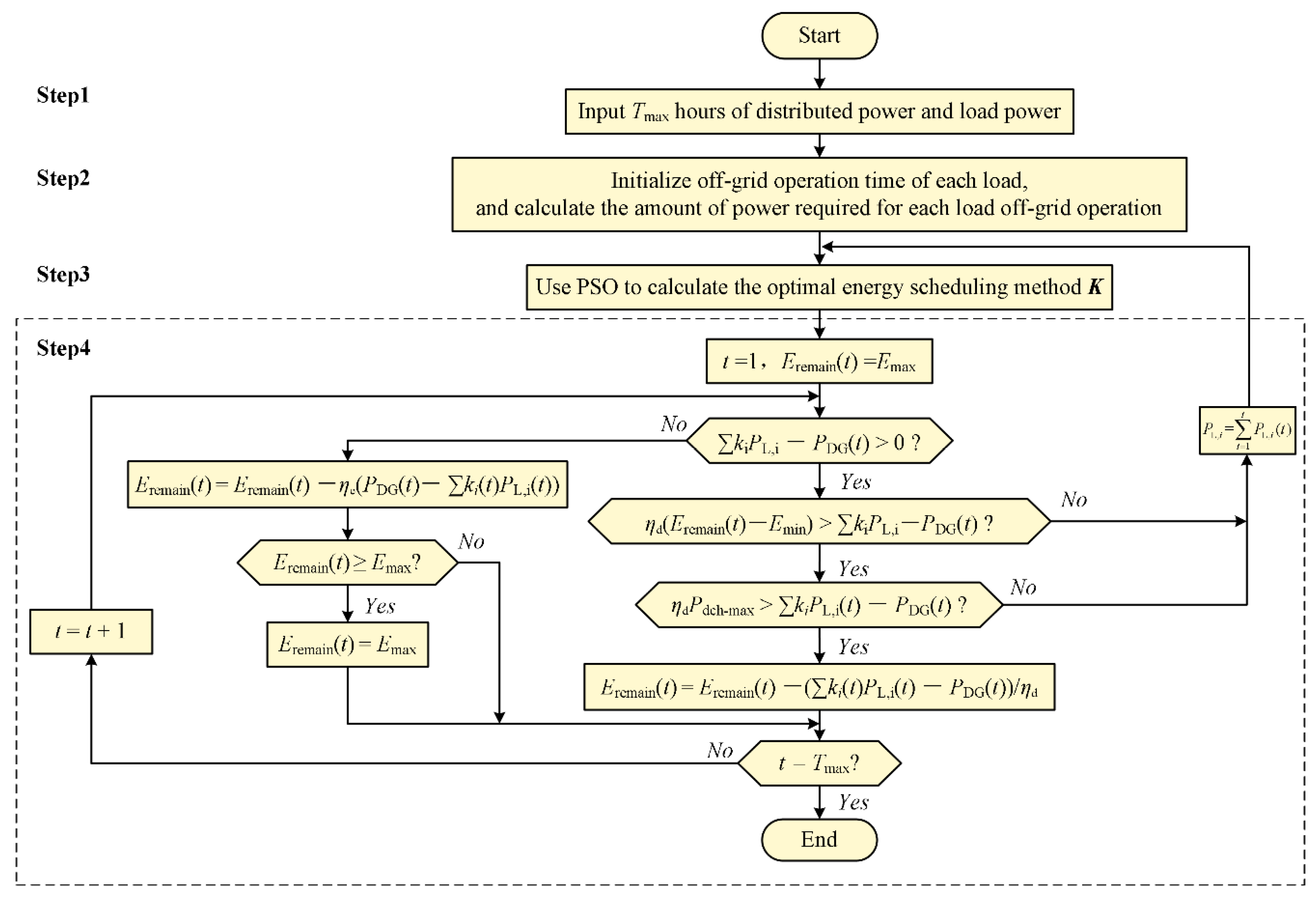
3.4. Optimization of Energy Dispatching by the Particle Swarm Optimization Algorithm

The PSO algorithm is a stochastic algorithm that can be optimized in a complex nonlinear solution space. It is concise and easy to operate without too much parameter adjustment. It has been widely used in various optimization problems [18,19]. The PSO algorithm is used to solve the energy scheduling optimization problem in this paper. Equations (13) and (14) are constraint conditions under the power supply region off-grid operation. During the calculation, K is corrected until constraints (13) and (14) are satisfied. The PSO algorithm is as follows:

Step 1: The period from the start of a power supply region’s off-grid operation to the recovery of grid-connected operation is $T_{\max }$, the weight coefficient of the load $i$ is ${\beta }_i$, and the minimum power supply degree of load $i$ is $k_{\mathrm{pt},i}(t)$. During load off-grid operation, the power of the DGs and each load are $P_{\mathrm{DG}}(1)$, $P_{\mathrm{DG}}(2)$, …, $P_{\mathrm{DG}}(T_{\max })$ and $P_{\mathrm{L},i}(1)$, $P_{\mathrm{L},i}(2)$, …, $P_{\mathrm{L},i}(T_{\max })$ respectively.

Step 2: Set all the load off-grid operation time is $T_{\max }$, the total power during the off-grid operation of each load $P_{\mathrm{L},i}$ can be calculated as follows:

$$P_{\mathrm{L},i}={\displaystyle \sum _{t=1}^{T_{\max }}{P}_{\mathrm{L},i}}(t)$$

(17)

Step 3: The relationship between the objective function and K is determined according to (8), (9), and (12), and then considering the constraints of (15) and (16), using the PSO algorithm to solve the energy scheduling optimization and obtain the optimal energy scheduling scheme $\mathit{K}=\left\{k_i\right\}$.

(a)

Initialize the number of particles in the particle group. For particle velocity V and position K, the i-th particle is p_i = (K_i, V_i). Initialize the individual extremum $pBest[i]$ and the global extremum $gBest$, initialize the iteration number as $\alpha =1$, and set the maximum number of iterations ${\alpha }_{\max }$.

(b)

According to the DGs and energy storage joint-power-supply model, calculate each particle’s adaptive value $Fit[i]$, that is, $\mathsf{\Delta }EENS$, using the previously described time sequence simulation. Then, correct the particle’s position $K_i$ and compare it with the individual extremum $pBest[i]$. If $Fit[i]<pBest[i]$, use $Fit[i]$ to replace $pBest[i]$. Then, compare $Fit[i]$ with the global extremum $gBest$. If $Fit[i]<gBest$, use $Fit[i]$ to replace $gBest$.

(c)

Update the velocity and position of the particle:

$$\{\begin{array}{l}{V}_{\mathrm{i}}=V_{\mathrm{i}}+c_1\times u_1\times \left(pBest\right[i]-K_{\mathrm{i}})+c_2\times u_2\times (gBest-K_{\mathrm{i}})\\ K_{\mathrm{i}}=K_{\mathrm{i}}+V_{\mathrm{i}}\end{array}$$

(18)

where $c_1$ and $c_2$ are learn factors, $u_1$ and $u_2$ are (0, 1) on the uniformly distributed random number, respectively.

(d)

Judge whether the number of cycles has been reached. If yes, the global extreme value $gBest$ is the value of $\mathsf{\Delta }EENS$, and the corresponding solution is power supply degree K. Otherwise, let $\alpha =\alpha +1$, and return to (b).

Step 4: According to the optimal scheduling scheme, the simulation method is used to simulate the off-grid operation status of the load, and judge whether there is a power shortage in the energy scheduling scheme:

(a)

Set the off-grid operation time to $t=1$, and the energy storage remaining power to $E_{\mathrm{remain}}(t)=E_{\max }$.

(b)

Judge whether $\sum k_i{P}_{\mathrm{L},i}-P_{\mathrm{DG}}(t)>0$. If the condition is met, go to the (c). Otherwise, accumulated charge power of energy storage $E_{\mathrm{remain}}(t)=E_{\mathrm{remain}}(t) +{\eta }_{\mathrm{c}}(P_{\mathrm{DG}}(t)-\sum k_i{P}_{\mathrm{L},i}(t))$, go to (e).

(c)

Judge whether ${\eta }_{\mathrm{d}}(E_{\mathrm{remain}}(t)-E_{\min }) >\sum k_i{P}_{\mathrm{L},i}-P_{\mathrm{DG}}(t)$. If the condition is met, go to the (d). Otherwise, cut off the load with the least weight coefficient in the off-grid operation load, use (19) to recalculate the load total demand power $P_{\mathrm{L},i}$ during the off-grid operation, and then return to Step 3.

$$P_{\mathrm{L},i}={\displaystyle \sum _{t=1}^t{P}_{\mathrm{L},i}}(t)$$

(19)

(d)

Judge whether ${\eta }_{\mathrm{d}}{P}_{\mathrm{dch}-\max }>\sum k_i{P}_{\mathrm{L},i}-P_{\mathrm{DG}}(t)$. If yes, accumulated the discharge power of energy storage, make $E_{\mathrm{remain}}(t)=E_{\mathrm{remain}}(t)-\frac{1}{{\eta }_{\mathrm{d}}}(\sum k_i{P}_{\mathrm{L},i}(t)-P_{\mathrm{DG}}(t))$, go to (f). Otherwise, cut off the load with the least weight coefficient in the off-grid operation load, use (19) to recalculate the load total demand power $P_{\mathrm{L},i}$ during the off-grid operation, and then return to Step 3.

(e)

Judge whether $E_{\mathrm{remain}}(t)\ge E_{\max }$. If yes, make $E_{\mathrm{remain}}(t)=E_{\max }$.

(f)

Judge whether $t=T_{\max }$. If yes, the load is changed to grid-connected operation, and this off-grid operation ends. Otherwise, the accumulated off-grid operation time is $t=t+1$, and return to (b).

The flow chart is shown in Figure 4.

4. Load Reliability Evaluation Based on the Hybrid Method

The load reliability by hybrid method is calculated in this paper. The reliability of load outside the power supply region and PCC are calculated by the GO method, and the reliability of load in the power supply region is calculated by MC simulation.

The hybrid method combines the advantages of the analytical method and MC simulation method. Firstly, the complex distribution network is equated with a simple radial main feeder network by the analytical method. Then, the MC simulation method is used to evaluate the reliability of the simplified distribution network. Compared with the traditional MC simulation method, this method significantly improves the simulation efficiency and calculation accuracy [20].

4.1. Using GO Method to Calculate Load Reliability outside the Power Supply Region

The load outside the power supply region is only powered by the power grid without DGs. Therefore, calculating the reliability of the load grid-connected operation does not require considering the influence of the DGs supply.

There are problems in modeling complexity and the difficulty in balancing the accuracy and speed of calculation when traditional analytical methods are applied to the reliability assessment of complex distribution systems. The GO method is used to calculate the reliability of the PCC and the load outside the power supply region in this paper. The method is a success-oriented system probability analysis technology to improve reliability calculation accuracy and speed [21,22,23]. Compared with the traditional analytic method, the GO method can fully consider the failure rate of switch action, the planned maintenance of the component, and the occurrence of multiple failures. According to the successful correlation between system devices, the reliability index of each load point is directly calculated.

When components in the distribution system, such as transformers and transmission lines, fail, the power grid can’t power to the load. The frequency probability $P$ and time probability $P_{\mathrm{U}}$ of each component’s equivalent operation are calculated as follows:

$$\{\begin{array}{l}P=1-\frac{\lambda }{N}\\ P_{\mathrm{U}}=1-\frac{\lambda \cdot r}{N}=1-\frac{U}{N}\end{array}$$

(20)

where $\lambda$ is the failure rate, $N$ is a time period (generally, 8760 h), $r$ is the average failure duration of a component, and $U$ is the component average power outage time.

For the load point $i$, the failure of the system components can be divided into three categories: (1) a component that requires repair can make the load restore the power supply, that is, the A class of components denoted as $N_1$; (2) a component whose fault can make the load restore the power supply by switching the switch, that is, the B class of components, denoted as $N_2$; and (3) a component that has no effect on the load, that is, the C class of components, denoted as $N_3$. The success probability coefficients $a_{\mathrm{A}}$ and $a_{\mathrm{B}}$ and the time probability coefficients $b_{\mathrm{A}}$ and $b_{\mathrm{B}}$ of the class A and B components relative to load $i$ are defined as follows:

$$a_{\mathrm{A}}={\displaystyle \prod _{i\in N_1}{P}_i},\hspace{1em}{b}_{\mathrm{A}}={\displaystyle \prod _{i\in N_1}{P}_{\mathrm{U},i}}$$

(21)

$$a_{\mathrm{B}}={\displaystyle \prod _{i\in N_2}{P}_i},\hspace{1em}{b}_{\mathrm{B}}={\displaystyle \prod _{i\in N_2}{P}_{\mathrm{U},i}}$$

(22)

Considering that the reliable operation rate of the circuit breaker is not 100%, the success probability coefficient $a_{\mathrm{C}}$ and the time probability coefficient $b_{\mathrm{C}}$ of the C class components are defined as follows:

$$\{\begin{array}{l}{a}_{\mathrm{C}}=1-(1-{\displaystyle \prod _{i\in N_3}{P}_i})(1-P_{\mathrm{b}})\\ b_{\mathrm{C}}=1-(1-{\displaystyle \prod _{i\in N_3}{P}_{\mathrm{U},i}})(1-P_{\mathrm{b}})\end{array}$$

(23)

where $P_i$ and $P_{\mathrm{U},i}$ are the successful operation of the frequency probability and time probability, and $P_{\mathrm{b}}$ is the circuit breaker reliable action probability.

According to (21) to (23), the reliability indexes of load point $n$ are defined as follows:

$$\{\begin{array}{c}\lambda =(1-a_{\mathrm{A}}{a}_{\mathrm{B}}{a}_{\mathrm{C}})N\\ U=(1-b_{\mathrm{A}}{b}_{\mathrm{B}}{b}_{\mathrm{C}})N\end{array}$$

(24)

4.2. Using the Monte Carlo Simulation Method to Calculate Load Reliability in the Power Supply Region

The DGs output in the power supply region has a random nature. The MC simulation method can be used to calculate multiple uncertain events through multiple random sampling. The MC simulation method is used to calculate the reliability of load in the power supply region in this paper.

After sampling the external equivalent component and the components in the power supply region with the MC method, it judges whether the power supply region off-grid operates successfully. It uses the PSO algorithm to solve the energy scheduling optimization, and calculates the load reliability in the power supply region with the obtained power supply degree K. The specific steps of the algorithm are as follows:

Step 1: Set the number of each load’s failure time $f[i]=0$, the outage time to $U\left[i\right]=0$ and the simulation time to $t=0$. Set the maximum simulation time $t_{\max }$.

Step 2: Generate a random number uniformly distributed on (0, 1) for the external equivalent component and each of the components within the power supply region. The time to failure (TTF) of each component is calculated as follows:

$$TT{F}_i=-(1/{\lambda }_i)\ln u$$

(25)

where $u$ is a random number uniformly distributed between (0, 1), and ${\lambda }_i$ is the annual average failure rate of the i-th component.

Step 3: Find the component with the smallest TTF, generate a random number uniformly distributed on (0, 1) for the component, and calculate the component’s time to repair (TTR):

$$TT{R}_i=-(1/{\mu }_i)\ln u$$

(26)

where ${\mu }_i$ is the repair rate of the i-th component.

Step 4: If the component is the external equivalent component, it can proceed as follows:

(a)

Generate a random number that is uniformly distributed on (0, 1), and calculate the success rate of off-grid operation to judge whether the power supply region successfully commences off-grid operation when the component faults.

(b)

If yes, generate a random number that is uniformly distributed on (0, 1), determine the time at which the fault occurred in a year, and calculate the power of the DGs and load in TTR hours from that moment.

(c)

According to the wind/solar/storage joint-power-supply and PSO algorithm, solve the energy scheduling optimization problem of the off-grid operation. According to the obtained K, accumulate the failure times outage time of the load in the power supply region.

If the component is not the external equivalent component, the outage time of the load is TTR, and the failure times and outage time of the load in the power supply region are calculated as follows: $f[i]=f[i]+1, U[i]=U[i]+TT{R}_i$. Proceed to Step 5.

Step 5: Calculate the simulation time: $time=time+TT{F}_i+TT{R}_i$.

Step 6: Judge whether $time>t_{\max }$. If yes, calculate the load point reliability index, and end the cycle. Otherwise, proceed to Step 2.

4.3. Calculating the Reliability of the Entire Network by the Hybrid Method

In this paper, the GO method is used to calculate the reliability of PCC and the load in the power supply region when the load is in grid-connected operation. MC simulation is used to sample the component and simulate the off-grid operation of the power supply region. The PSO algorithm is used to solve the energy scheduling optimization problem. Then, according to the obtained K or TTR, the failure times and outage time of each load are calculated. Finally, the load reliability of the entire network is calculated.

The evaluation process of the hybrid method is shown in Figure 5.

5. Case Study

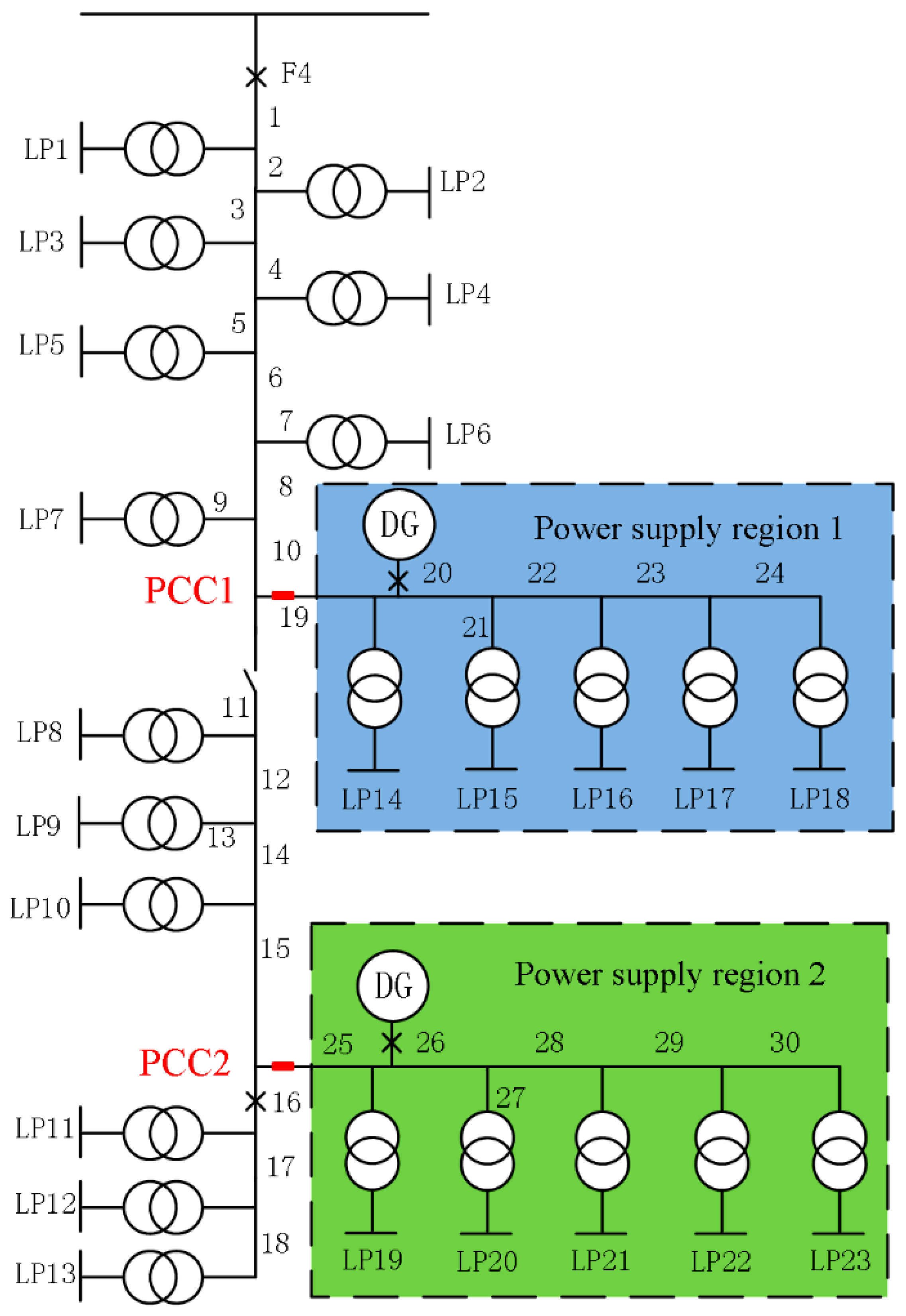
5.1. The Example System Parameters

The Feeder 4 RBTS BUS6 system [24] is adopted as a test system in this paper. The example electricity distribution network is shown in Figure 6.

The feeder consists of 30 lines, 23 load points, 23 fuses, 23 transformers, 4 circuit breakers, and 1 isolating switch. The reliable action rate of the circuit breaker is 80%, the reliable operation rate of the fuse is 100%, the failure rate of the line is 0.065 f/km-year, the repair time of each line is 5 h, the transformer failure rate is 0.015 f/km-year, the repair time is 200 h, and the operation time of the isolating switch is 1 h.

In the power supply region 1 and the power supply region 2, there is a DG composed of a wind/solar/storage joint-power-supply system. The parameters of the two DGs are the same. The WT rated power is 1.5 MW. The cut-in, cut-out, and rated wind speed are 2.5, 22 and 10.5 m/s, respectively. The maximum output power of PV is 1.5 MW; the $\alpha$ and $\beta$ are 0.230 and 0.915, respectively. The storage capacity is 2 MW, energy storage charge and discharge efficiency ${\eta }_{\mathrm{c}}$ and ${\eta }_{\mathrm{d}}$ are 80%. The weight coefficient of the load outside the power supply region is 1.0. The minimum power supply degree of the load in the power supply region is 0.8.

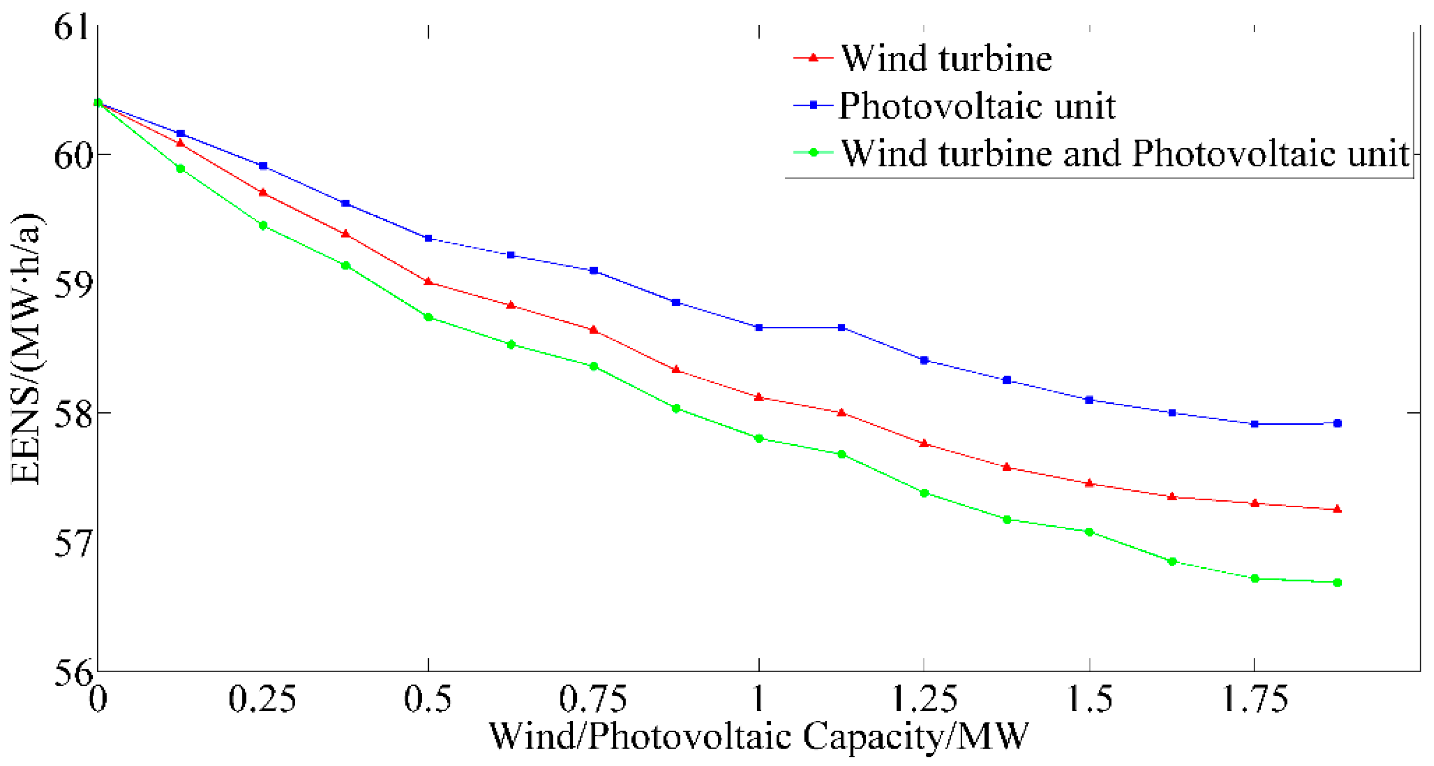
5.2. The Influence of DG Capacity on System Reliability Index

This paper uses reliability index EENS to study the influence of DGs capacity on system reliability index.

The capacity of the energy storage system is unchanged at 2 MW. The load classification, load reduction, and energy scheduling are not considered. The EENS changes with the capacity of the WT and the PV as shown in Figure 7. The three groups in Figure 7 are WT, PV, and WT + PV, where the capacity of the WT and PV is the value corresponding to the abscissa. In the group of WT + PV, the capacity of the WT is the same as the capacity of PV, whose capacity is the value corresponding to the abscissa.

From the Figure 7, it can be seen that the addition of DGs can improve system reliability. In the initial stage, DGs have more obvious effect on reliability improvement. When DGs capacity increases continuously, the effect of system reliability improvement gradually saturates. In this example, the effect of WT on reliability improvement is better than that of PV.

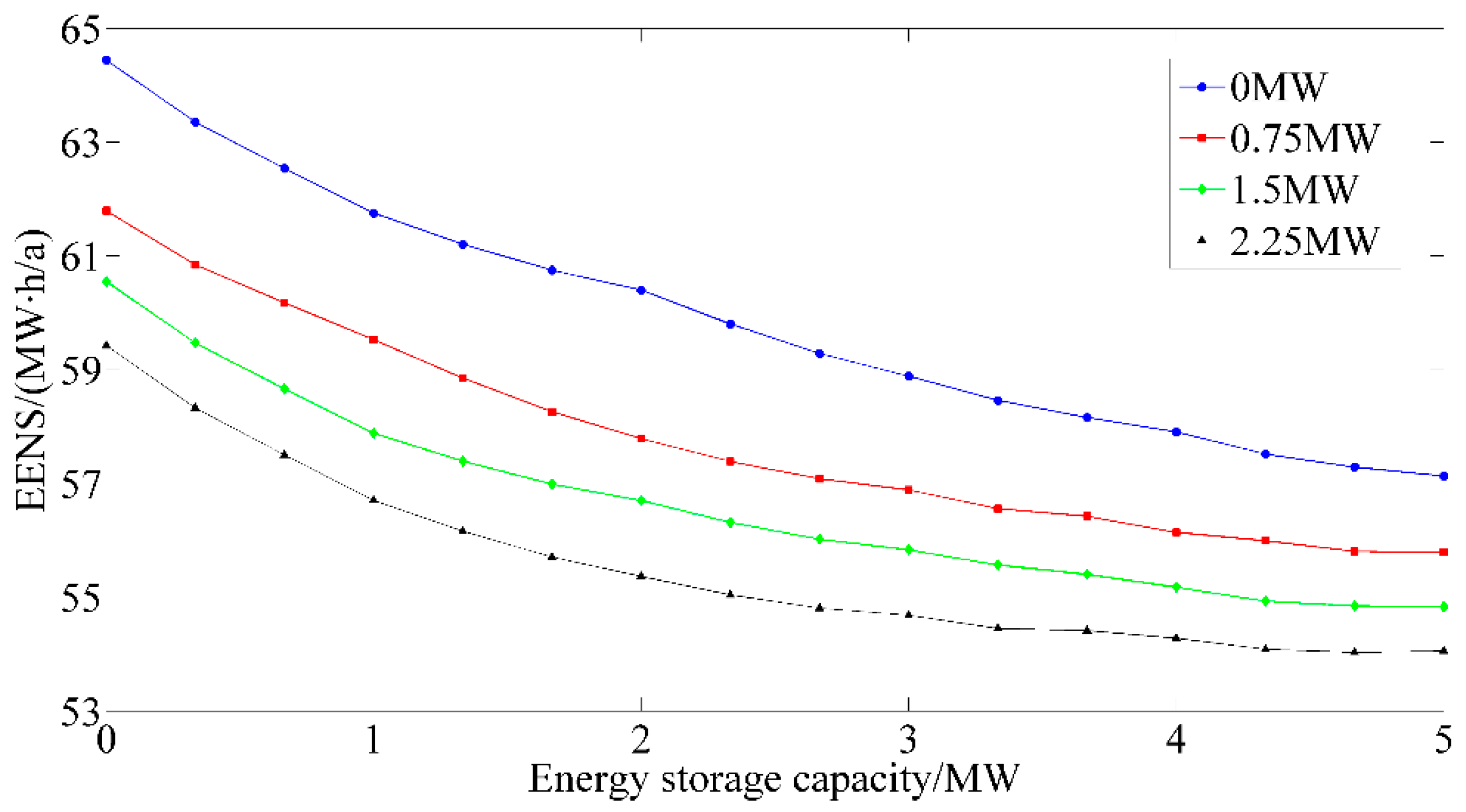
The EENS of the system, calculated by taking several sets of different WT + PV capacity combinations from Figure 7, can be shown in Figure 8.

From Figure 8, it can be seen that the EENS decline in the initial stage of the energy storage joining system is obvious. As the capacity of energy storage systems continues to increase, the rate of decline in EENS tend to be flat. The impact of EENS on the WT+PV capacity is also decreasing. When the capacity of the energy storage increases, the EENS decreases stably. It can reflect the characteristics in that the energy storage can smooth the random output of the DG to improve the power supply quality.

5.3. Reliability Index of a Different Energy Scheduling Scheme

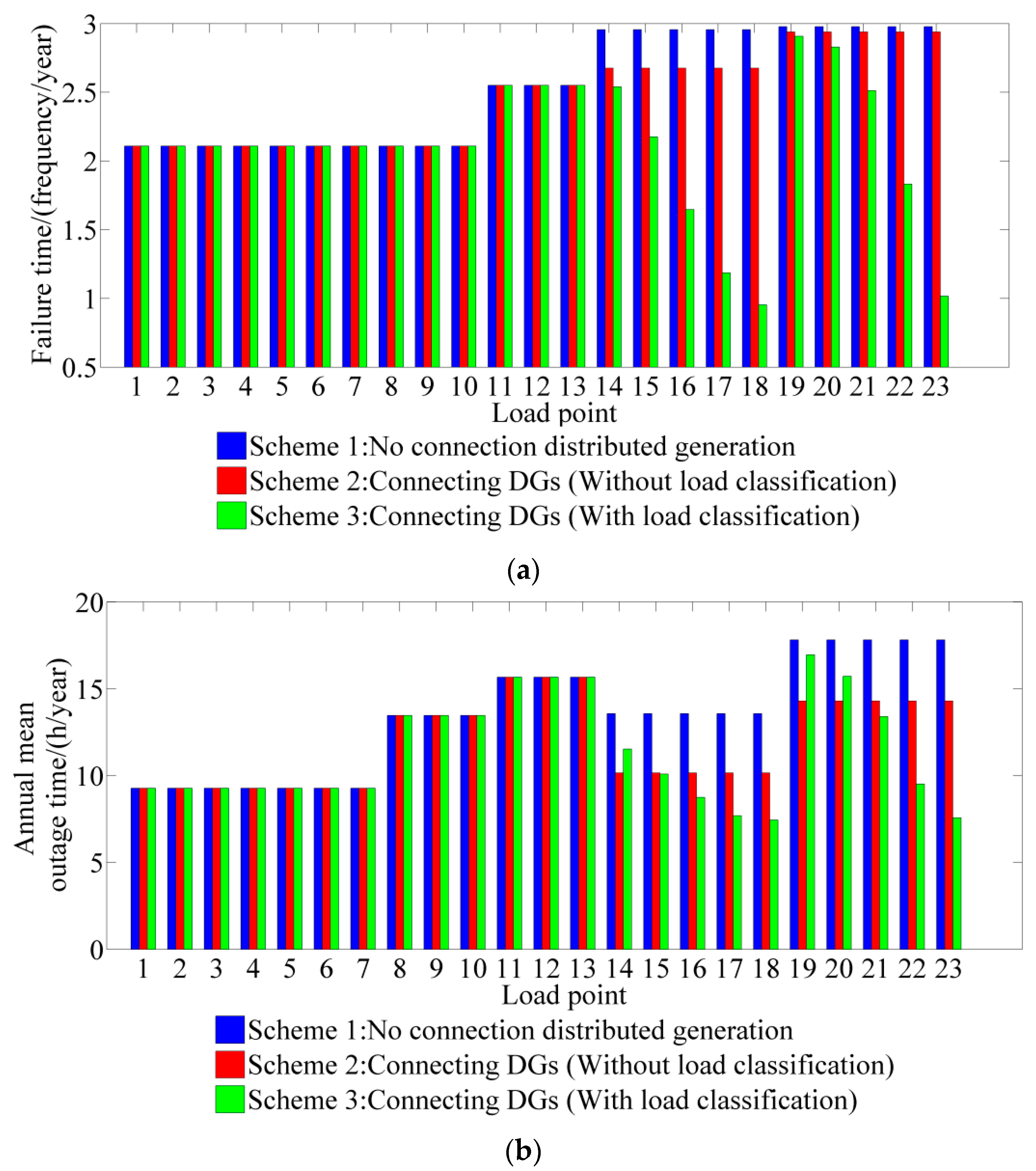
According to the hybrid method evaluation process, the reliability evaluation of the distribution network with DG is performed in three schemes:

Scheme 1: no connecting DGs in the distribution network.

Scheme 2: connecting DGs in the distribution network, no weight coefficient is set for the load, and all load weight coefficient are the same.

Scheme 3: connecting DGs in the distribution network and the weights for the load are set. In the power supply region 1, the weights for loads 14, 15, 16, 17, and 18 are 1.0, 1.05, 1.1, 1.2, and 1.3 respectively. In the power supply region 2 the weights for loads 19, 20, 21, 22, and 23 are 1.0, 1.05, 1.1, 1.2, and 1.3 respectively.

Through the described model and algorithm, the reliability index of each load point and the entire system are calculated. Figure 9 and

Table 1. System Reliability Indexes.

Reliability Index	Scheme 1	Scheme 2	Scheme 3
	Traditional Algorithm	Traditional Algorithm	Traditional Algorithm	Modified Algorithm
SAIFI/(f/system customer)	2.394	2.351	2.199	2.191
SAIDI/(h/customer)	12.353	11.436	11.300	11.260
ASAI/%	0.9986	0.9987	0.9987	0.9987
EENS (MWh/year)	64.034	56.693	52.964	52.227

list the reliability indexes of the load points and the reliability indexes of the system, respectively.

As shown in Figure 9, loads 1 to 13 are load points outside the power supply region, and their reliability is not affected by DGs.

Based on the results of scheme 1 and scheme 2 in Figure 9 and Table 1, it can be observed that after accessing the DGs, the failure rate and the annual average outage time of the load point in the power supply region are reduced. This outcome indicates that the access of the DGs can effectively improve load reliability. Compared with the reliability of the load points in scheme 2 and scheme 3, more power can be allocated for the load with a larger weight coefficient and their reliability is improved. Less power will be allocated and the reliability will be reduced for the load with a small weight coefficient. Compared with the traditional algorithm and modified algorithm in Scheme 3, the modified reliability indexes can improve the effect of the large weight coefficient load on the system reliability, which improves system reliability and verifies the effectiveness of the proposed method.

5.4. Comparison of Load Reliability Indexes with Different Classification Numbers

Taking the power supply region 2 as an example, the load reliability indexes with different classification numbers are studied. Under the condition of the same equivalent load, the weight coefficient of the load is changed, and energy scheduling optimization is adopted to compare load reliability with different classification numbers.

Scheme 1: the load in the power supply region is divided into two types according to degree of importance as follows: loads 19, 20, 21: weight coefficient 1.0; loads 22 and 23: weight coefficient 1.488;

Scheme 2: the load in the power supply region is divided into three types according to degree of importance as follows: loads 19 and 20: weight coefficient 1.0; load 21: weight coefficient 1.20; loads 22 and 23: weight coefficient 1.36;

Scheme 3: the load in the power supply region is divided into four types according to degree of importance as follows: loads 19 and 20: weight coefficient 1.0; load 21: weight coefficient 1.20; load 22: weight coefficient 1.30; load 23: weight coefficient 1.40.

The load reliability index in the power supply region is shown in

Table 2. System Reliability Indexes.

Scheme	Load	Weight Coefficient	Outage Time/(f/year)	Annual Mean Outage Time/(h/year)
1	LP19	1.0	2.843	16.465
	LP20	1.0	2.814	16.050
	LP21	1.0	2.874	16.517
	LP22	1.49	1.602	8.775
	LP23	1.49	1.429	8.158
2	LP19	1.0	2.877	17.123
	LP20	1.0	2.870	16.734
	LP21	1.2	2.696	14.984
	LP22	1.36	1.770	9.185
	LP23	1.36	1.280	7.893
3	LP19	1.0	2.927	17.343
	LP20	1.0	2.921	17.058
	LP21	1.2	2.684	14.775
	LP22	1.3	2.003	10.146
	LP23	1.4	1.082	7.533

.

As shown in Table 2, the difference in load reliability with the same weight coefficient is small, and the difference in load reliability with a different weight coefficient is large. The larger the load weight coefficient is, the more power is allocated in the energy scheduling and the higher the reliability. Therefore, we can set a large weight coefficient for an important load to meet a demand for priority power supply for that load.

5.5. Comparison of Load Reliability Indexes with Different Capacity Ratios

Taking the power supply region 2 as an example, the load reliability indexes with different capacity ratios are studied. In the case of energy scheduling optimization, the influence of different capacity ratios in different load classes on load reliability is discussed under the condition of the same load classification number as follows:

Scheme 1: the load in the power supply region is divided into two types according to degree of importance: loads 19, 20, 21: weight coefficient 1.0, accounting for 58% of the total load; loads 22 and 23: weight coefficient 1.4, accounting for 42% of the total load;

Scheme 2: the load in the power supply region is divided into three types according to degree of importance: loads 19 and 20: weight coefficient 1.0, accounting for 32% of the total load; loads 21, 22, and 23: weight coefficient 1.4, accounting for 68% of the total load;

Scheme 3: the load in the power supply region is divided into four types according to degree of importance: load 19: weight coefficient 1.0, accounting for 14% of the total load; loads 20, 21, 22, and 23: weight coefficient 1.40, accounting for 86% of the total load.

The load reliability indexes in the power supply region are shown in

Table 3. System Reliability Indexes.

Scheme	Load	Weight Coefficient	Capacity Ratio	Outage Time (f/year)	Annual Mean Outage Time (h/year)
1	LP19	1.0	58%	2.31	11.519
	LP20	1.0		2.328	12.137
	LP21	1.0		2.339	11.626
	LP22	1.4	42%	0.915	7.498
	LP23	1.4		0.915	7.498
2	LP19	1.0	32%	2.585	14.777
	LP20	1.0		2.397	13.386
	LP21	1.4	68%	1.379	7.913
	LP22	1.4		1.162	7.728
	LP23	1.4		0.995	7.472
3	LP19	1.0	14%	2.632	15.544
	LP20	1.4	86%	1.531	9.032
	LP21	1.4		1.714	8.708
	LP22	1.4		1.846	9.427
	LP23	1.4		1.400	8.389

.

As shown in Table 3, in scheme 1, the load ratio of 1.2 is 42%, the failure rate of load 22 is 1.611 f/year, and the annual mean outage time is 8.692 h/year. In scheme 3, the load ratio of 1.2 is 86%, the failure rate of load 22 is 2.210 f/year, and the annual mean outage time is 11.979 h/year. It indicates that load 22 in scheme 1 has a higher reliability. The total power of the important load increases, and the average power allocation of each load is reduced. Then the reliability is reduced. For a load with a weight coefficient 1.0, such as load 19 in scheme 1, the failure rate is 2.831 f/year and the annual mean outage time is 16.357 h/year. In scheme 3, the load 19 failure rate and annual mean outage time are 2.950 f/year and 17.540 h/year, respectively. The output power of DGs and energy storage are mostly allocated to important loads, and the amount of loads assigned to a small weight coefficient is small. In order to improve the reliability of important loads, a reasonable weight coefficient should not only be set but also the proportion of various types of load should be considered.

6. Conclusions

This paper establishes a reliability model of DGs and an energy storage joint-power-supply based on modified load reliability indexes according to load classification, which have improved the reliability indexes of the load and system. The PSO algorithm is used to solve the optimal energy scheduling problem, and load reliability indexes under different load scheduling schemes, classification numbers, and capacity ratios are compared. The research shows the following:

(1)

In off-grid operation, DGs can supply the load in the power supply region to improve load reliability.

(2)

Through load classification and energy scheduling optimization, in the case of the same equivalent load, the larger the weight coefficient is, the more power is allocated and the higher the reliability.

(3)

In the power supply region, when the total load capacity and the weight coefficient are the same, the difference in the capacity ratio can affect the load reliability.