Power and Capacity Consensus Tracking of Distributed Battery Storage Systems in Modular Microgrids

Abstract

Conventional microgrids have a specific system configuration and a complex hierarchical control structure, which has resulted in difficulties in their economic development. A modular microgrid based on distributed battery storage has been proposed to realize the rapid economic development of small-to-medium microgrids. Control of modular microgrids is simplified to voltage control within modules and exchange power control among modules. Battery power has great influence on battery performance. Space-time complementary power characteristics among modules help to alleviate power fluctuations, prolong the service life and realize the unified maintenance of distributed batteries. Leader-following consensus theory of multi-agent systems is adopted to realize the power and capacity consensus tracking of distributed battery storage in a modular microgrid. Sufficient and necessary conditions for continuous-time and sampled-data bounded power and capacity consensus tracking of distributed battery storages are deduced by a matrix analytical method. Steady regions of sampling period and sampling delay for sampled-data bounded power and capacity consensus tracking are determined by analytical or numerical solutions. Simulations and experiments on a modular microgrid demonstration project located on DongAo Island (China) show the effectiveness and robustness of the proposed power and capacity consensus tracking strategy for distributed storage systems. The power and capacity consensus tracking strategy determines the exchange power among modules and improves the control technology of modular microgrids.

1. Introduction

Microgrids are an effective way to realize the large-scale integrated utilization of renewable energy sources, such as wind and solar power. Microgrids can be integrated into the distribution network as a flexible and controllable part, or run as stand-alone power systems to provide energy supply for areas which are unreachable by the regular utility grid [1]. With the reform of the electricity market, the application of microgrids is booming [2], and a large number of microgrid projects have been built around the world. An off-grid microgrid with installed capacity 357 kW was developed on the Isle of Eigg in Scotland to provide a reliable 24-h electricity supply to the islanders [3]. A 400 kW microgrid comprising four 100 kW hybrid combined cooling heating and power (CCHP), uniquely able to seamlessly transition between grid-tie and island-mode operation, provides power, water and heat for the Brevoort building in New York [4]. A megawatt demonstration project located on Nanji Island in China was also developed to provide clean energy [5]. With the development of sustainable buildings, home microgrids with installed capacities of tens of kilowatts also represent an attractive way to save building energy [6,7].

The system capacity of the abovementioned microgrid projects varies greatly and therefore their configuration and operation mode also differ accordingly. Some microgrids can operate only in grid connected mode and microsources usually work in power control mode [8,9]. Some microgrids can operate only in the islanding mode and microsources work with a master-slave control or with the droop control [10,11]. Some microgrids are able to operate in both on-grid and off-grid mode [12], which need mode transition control. Based on the experimental microgrid built at the Prince—Electrical Energy System Lab of the Polytechnic of Bari (Italy), the main technical issues on five operation modes and five transitions were examined and implemented in detail [13,14]. Appropriate control is a prerequisite for stable, economical and efficient operation of a microgrid. In order to standardize the design of control systems, a three-layer hierarchical control scheme derived from ISA-95 is presented in [15,16]. The primary control based on the droop method adjusts the voltage reference provided to the inner current and voltage control loop [17]. The secondary control restores the deviations produced by the primary control and distributed coordinated control strategy ensuring voltage tracking and power sharing is applied [18]. The tertiary control is the optimum energy management of microgrid and various optimum methods such as Model Predictive Control [19,20], Conditional Value at Risk [21], Dynamic Programming [22], Flower Pollination Algorithm [23] and Particle Swarm Optimization [24] are adopted. The conventional configuration and control of microgrids mimics a large-scale power system AC grid, which may be applicable to large capacity microgrids, but is too complicated and expensive for a small-to-medium microgrid.

In order to realize the rapid economic development of small-to-medium microgrids, we have carried out a series of studies on stand-alone microgrid technology suitable for island applications. Power supply becomes a major problem with the exploitation of islands. The traditional power system on islands is the diesel generator, which generates noise and air pollution. Island ecology is usually very fragile and it is urgent to use clean energy. A stand-alone modular microgrid based on distributed batteries was proposed in [25], which can realize easy and economic networking. Each module has the same hardware configuration, composed of wind and solar power, battery storage, loads and converters. Modules are connected to the microgrid through a converter and so the AC bus of the modular microgrid is segmental. Accordingly the control of the modular microgrid is simplified to the voltage control within modules and exchange power control among modules. Voltage control within modules has been discussed in detail [26,27,28], but how to determine exchange power among modules still needs to be studied in depth according to different optimum objectives.

Battery storage systems are the energy and power balancing units in a modular microgrid. Nowadays the most widely used storage systems are electrochemical energy storage units such as lead-acid batteries or lithium-ion batteries. Battery lifespan is closely related to the charge and discharge power, the depth of discharge, charge/discharge cycle times and so on [29]. The existing battery lifespan prediction models are all established on regular charge and discharge processes [30]. Battery power in a modular microgrid compensates for the unbalanced power between generation and load. Because wind and solar power and loads are intermittent and random, the battery power fluctuates violently, which deteriorates the power quality and results in difficulties for lifespan prediction [31]. When the battery power is different, some battery storage systems will be out of service due to exceeding the capacity limit, which leads to the unexpected reconfiguration of a modular microgrid. Modules are distributed in different locations and there exists space-time complementary power characteristics among modules, which helps to alleviate the battery power fluctuations. Therefore power and capacity consensus tracking of distributed battery storage is necessary to improve the power quality and realize the unified maintenance of battery storage systems.

Each module is free to work in on-grid mode or off-grid mode, which leads to the reconfiguration of the microgrid, and so a decentralized power and capacity consensus control scheme should be adopted [32]. Multi-agent consensus theory based on a sparse communication network is an appropriate tool for analyzing and designing a distributed system [33]. Chow first proposed an incremental cost consensus algorithm to solve the conventional centralized economic dispatch problem in a smart grid [34] and the relationship between the convergence rate and network topology has been discussed in [35]. Yu put forward a virtual generation tribe-based consensus algorithm for dynamic generation dispatch of smart grids [32]. A fully distributed coordination control scheme including containment and consensus-based algorithm is proposed realizing a good coordination between reactive power sharing and voltage bound in an AC microgrid [36]. The above- mentioned multi-agent consensus studies on smart grids or microgrids mainly concentrate on the design of consensus protocols, communication network topologies, and proof of convergence with continuous-time. The actual control system is a sampled-data control system based on a digital processor. The information is transmitted only at the sampling time. Sampling and communication delays always exist, which has a great influence on the stability and the convergence rate of multi-agent systems. We have carried out a series of theoretical researches on bounded consensus tracking of multi-agent systems with sampled-data [37,38], which lays a good foundation to design a power and capacity consensus tracking strategy for distributed battery storage in a modular microgrid.

The configuration and operation mode of a modular microgrid are introduced first. Then the power relationships of a modular microgrid are analyzed and a multi-agent power and capacity model of distributed battery storage with an undirected communication network can be established. The continuous-time and sampled-data control protocols are designed based on the leader-following consensus tracking theory. The sufficient and necessary conditions for bounded power and capacity consensus tracking of distributed batteries are derived by a matrix analytical method and the steady regions of sampling period and sampling delay can be determined by analytical or numerical solutions. Simulations and experiments are then conducted on the modular microgrid demonstration project on DongAo Island (China).

The main contribution of this paper is that power and capacity consensus tracking of distributed battery storage is chosen as an optimum control objective, which can make full use of the space-time complementary power characteristics among modules, to alleviate the power fluctuations and realize the unified maintenances of distributed battery storage systems. Leader-following consensus tracking theory of multi-agent systems is adopted to study the continuous-time and sampled-data control protocols and stabilization ranges of parameters. The power and capacity consensus tracking strategy of distributed battery storage determines the exchange power among modules and therefore the control problem of the modular microgrid is solved completely. The power and capacity consensus tracking strategy improves the control technology of a modular microgrid and promotes the economic application of small-to-middle modular microgrids.

The organization of this paper is as follows: Section 2 illustrates the modular microgrid. Section 3 introduces leader-following consensus tracking theory of multi-agent systems. Section 4 discusses our continuous-time power and capacity consensus tracking strategy of distributed battery storage systems. Section 5 discusses sampled-data power and capacity consensus tracking strategy of distributed battery storage. Section 6 presents simulations and experiments on the modular microgrid demonstration project on DongAo Island. Section 7 discusses the conclusions.

2. Modular Microgrid

DongAo Island is a classic tourist island, located in Zhuhai City, Guangdong Province of Southern China, with an area of 4.66 square kilometers and a permanent population of more than 600 people. The original diesel generator power supply system on the island had a series of drawbacks such as poor power quality, high electricity price and no guarantee of uninterruptible power supply. There are abundant wind and solar resources and so the original diesel generator power system should be converted to a renewable energy microgrid.

2.1. System Configuration

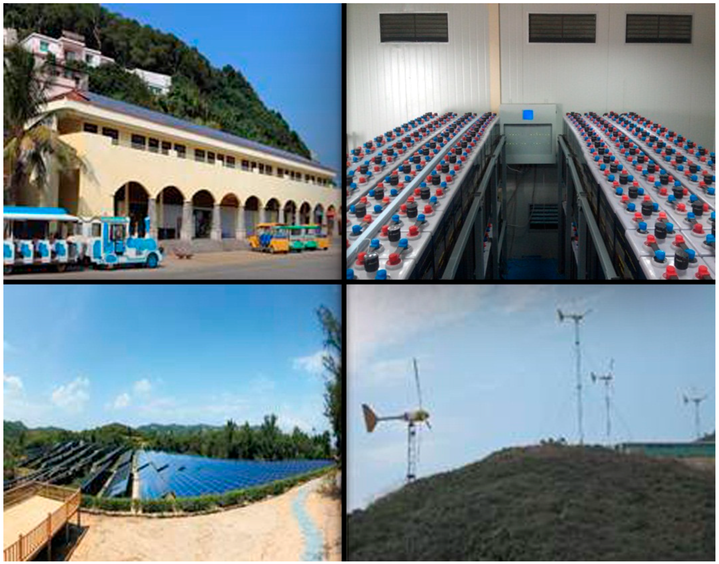
In order to realize power generation and consumption on the spot reducing the power transmission loss, photovoltaic (PV) arrays and wind turbines are installed in the concentrated load zones. Figure 1 shows the battery storage system, rooftop PV, terrestrial PV and wind turbines installed on DongAo Island. The structure of the modular microgrid on DongAo Island is shown in Figure 2. There are three concentrated load zones on DongAo Island and three modules are established. Module 1 is the power plant zone. Module 2 is the comprehensive building zone and module 3 is the cultural center zone. Each module is an autonomous energy system and has the same configuration, which is composed of wind and solar generation, battery storage, load and power electronic converter. Modules are interconnected through the 10 kV transmission network by transformers. Each module can freely access or separate from the grid. Module 0 is composed of three-porter converter, battery storage and diesel generator. Module 0 works as V/F voltage source establishing the 10 kV voltage of the transmission network. The diesel generator in Module 0 is a backup source and works only when the renewable energy is not enough.

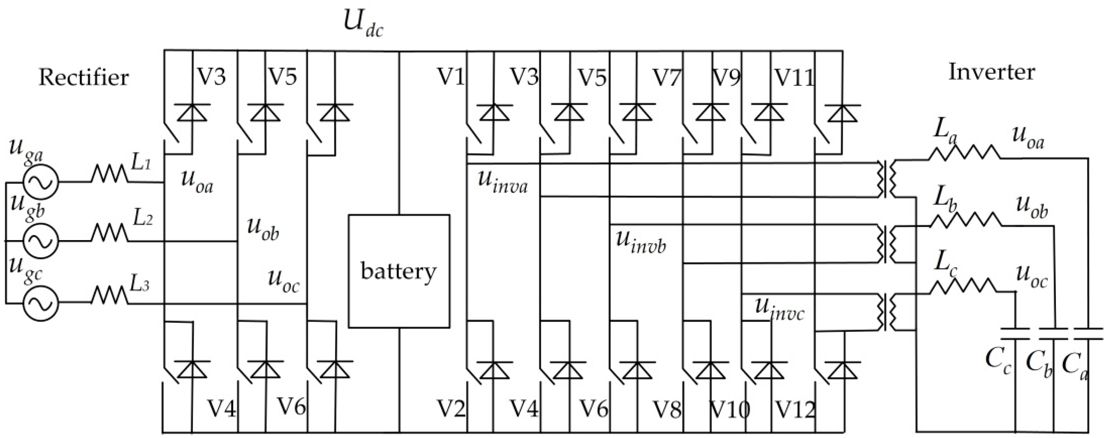
A three-port converter is the key equipment for the configuration and control of a modular microgrid. It has AC-DC-AC topology. The 480 V battery pack composed of 240 2-Volt cells in series is connected to the DC port. The AC-DC part connected to the transformer works as a rectifier in active power and reactive power (PQ) control mode and realizes the three-phase balanced bidirectional power flow between module and microgrid. When the module has surplus energy, it releases energy to the microgrid. When the energy is insufficient, the module absorbs energy from the microgrid. The other DC-AC inverter part is only responsible for establishing the voltage reference within the module. Because of the isolation of three-port converter, the AC bus of the modular microgrid is segmental, so control of the modular microgrid is simplified to the voltage control within modules and exchange power control among modules. The adopted topology of three-port converter is shown in Figure 3. The inverter with three-phase four-wire structure can realize three-phase balanced output voltage even under nonlinear or unbalanced load conditions and has been discussed in detail in [25].

2.2. Power Relationship of Modular Microgrid

Because the diesel generator acts only as a backup source, diesel generator power is not considered in this paper. Power transmission loss and power conversion loss are neglected and the power flow chart of modular microgrid is shown in Figure 4 according to Figure 2.

2.2.1. Power Balance in the Module

$$P_{Bati}(t)=P_{Ei}(t)+P_{PVi}(t)+P_{WTi}(t)-P_{LDi},i=1,2,3$$

(1)

where $P_{Bati}$ is positive for charging power and negative for discharging power of battery, $P_{PVi}$ is the solar power, $P_{WTi}$ is the wind power, $P_{LDi}$ is the load power, and $P_{Ei}$ is the exchange power between module i and microgrid. The dynamics of battery power are:

$$d{P}_{Bati}(t)/dt=d{P}_{Ei}(t)/dt+d{P}_{PVi}(t)/dt+d{P}_{WTi}(t)/dt-d{P}_{LDi}/dt,\hspace{0.17em}i=1,2,3$$

(2)

where $P_{PVi}$, $P_{WTi}$ and $P_{LDi}$ are uncontrollable random perturbation variables, so $P_{Ei}$ is chosen as the control variable and $P_{Bati}$ can be regulated by $P_{Ei}$.

The unit of battery power is kW and the unit of battery capacity is kWh. The relationship between battery capacity and battery power can be expressed as:

$$S_{Bati}\left(t\right)=\frac{{\displaystyle \int P_{Bati}dt}}{3600}.$$

(3)

2.2.2. Power Balance among Modules

$$P_{Bat0}(t)=P_{E0}(t)=-P_{E1}(t)-P_{E2}(t)-P_{E3}(t)$$

(4)

Because Module 0 works as a voltage source, $P_{E0}$ is a power slack node and is determined by the exchanged powers of other modules.

3. Leader-Following Consensus Tracking Theory of Multi-Agent Systems

Figure 5 shows the undirected communication network of leader-following multi-agent system [39]. Node set V = {1, 2,…, n} represents independent agents. Weighted adjacent matri $A=\left[a_{ij}\right]$ describes the relationship between nodes. If there exists information communication between agent i and j, $a_i{}_j>0$, otherwise $a_i{}_j=0$. For an undirected network, its adjacent matrix A is a symmetric matrix and $a_{ij}=a_{ji}$. Laplacian matrix L = [$l_{ij}$] is another matrix describing the network topology and the element is:

$$1_{ij}=\{\begin{array}{cc}-a_{ij}& i\ne j\\ {\displaystyle {\sum }_{j\ne i}{a}_{ij}}& i=j\end{array}$$

(5)

If there is a leader in a multi-agent system, agent 0 presents the leader. The leader adjacent matrix is defined as B = diag $\left(b_1,b_2,\dots ,b_n\right)$. If there exists information communication between agent i and the leader, the leader adjacent element $b_i>0$, otherwise $b_i=0$.

The dynamic characteristics of first-order multi-agent system can be described as [40]:

$$d{x}_i\left(t\right)/dt=u_i\left(t\right),i\in I$$

(6)

where $x_i$ is the state of the agent and $u_i$ is the control variable. To ensure that all the agents can follow the leader’s reference state, Wei presented a typical continuous-time consensus tracking protocol [40]:

$$u_i\left(t\right)=b_i\left(x_0\left(t\right)-x_i\left(t\right)\right)+{\displaystyle {\sum }_{j=1}^n{a}_{ij}\left(x_j\left(t\right)-x_i\left(t\right)\right),i=1,2,\dots n.}$$

(7)

where $x_0$, $x_i$, $x_j$ are states of the leader agent, agent i and agent j individually.

Through the periodic sampling technique, the sampled-data control model of Equation (6) is:

$$x_i\left(kT+T\right)=x_i\left(kT\right)+T{u}_i\left(kT\right),\hspace{0.17em}k=0,1,2,\dots ,i=1,2,\dots n.$$

(8)

where T is the sampling period and k is the discrete time index.

When time delay is not considered, the control input can be expressed as:

$$u_i\left(kT\right)=-b_i\left(x_i\left(kT\right)-x_0\left(kT\right)\right)+{\displaystyle {\sum }_{j=1}^n{a}_{ij}\left(x_j\left(kT\right)-x_i\left(kT\right)\right)}$$

(9)

Lemma 1.

Consider an undirected network topology composed of n agents, the leader is globally reachable only when the Hermite matrix H = B + L is positive definite. That means all the eigenvalues of H have a positive real part$Re\left({\lambda }_i\left(H\right)\right)>0$ [41].

Lemma 2.

All the roots of equation $\left(1+a+b\right)\times t^2+2\left(1-b\right)\times t+1-a+b=0$ are in the left half open plan only when all the eigenvalues of equation $s^2+as+b=0$ are located in the unit circle. a and b are real numbers [42].

Lemma 3.

Suppose matrix $P=\left[\begin{array}{cc}A& B\\ C& D\end{array}\right]$ is m + n order matrix, where A is m-order square matrix and D is n-order square matrix, B is m × n matrix and C is n × m matrix. The determinant of block matrix P.

(1) 

$\left|P\right|=\left|\begin{array}{cc}A& B\\ C& D\end{array}\right|=\left|A\right|\cdot \left|D-C{A}^{-1}B\right|$when matrix A is an invertible matrix.

(2) 

$\left|P\right|=\left|\begin{array}{cc}A& B\\ C& D\end{array}\right|=\left|D\right|\cdot \left|A-B{D}^{-1}C\right|$when matrix D is an invertible matrix.

4. Continuous-Time Power and Capacity Consensus Tracking Strategy of Distributed Battery Storages

In order to develop a universal model, n following modules are considered. According to Equations (2), (6) and (7), the continuous-time power and capacity consensus tracking protocol of battery storage is:

$$u_i\left(t\right)=\frac{d{P}_{Ei}}{dt}=b_i\left(P_{Bat0}-P_{Bati}\right)+{\displaystyle {\sum }_{j=1}^n{a}_{ij}\left(P_{Batj}-P_{Bati}\right)}+k_i\left(S_{Bat0}-S_{Bati}\right)+{\displaystyle {\sum }_{j=1}^n{k}_{ij}\left(S_{Batj}-S_{Bati}\right)}.$$

(10)

where b_i and a_ij are adjacent coefficients of battery power network, k_i and k_ij are the adjacent coefficients of battery capacity network:

Let $\widehat{P_{Bati}}=P_{Bati}-P_{Bat0}$, $\widehat{S_{Bati}}=S_{Bati}-S_{Bat0}$, $P_{xi}=-\frac{d{P}_{Bat0}}{dt}+\frac{d{P}_{PVi}}{dt}+\frac{d{P}_{WTi}}{dt}-\frac{d{P}_{LDi}}{dt}$, then $\widehat{P_{BAT}}={(\widehat{P_{Bat1}},\widehat{P_{Bat2}},\dots ,\widehat{P_{Batn}})}^T$, $\widehat{S_{BAT}}={(\widehat{S_{Bat1}},\widehat{S_{Bat2}},\dots ,\widehat{S_{Batn}})}^T$, $P_X={(P_{x1},P_{x2},\dots ,P_{xn})}^T$. The dynamics of consensus variables $P_{Bati}$ and $S_{Bati}$ are:

$$\left[\begin{array}{c}d\widehat{P_{Bat}}/dt\\ d\widehat{C_{Bat}}/dt\end{array}\right]=G\left[\begin{array}{c}\widehat{P_{Bat}}\\ \widehat{C_{Bat}}\end{array}\right]+\left[\begin{array}{c}\widehat{P_x}\\ 0\end{array}\right].$$

(11)

where:

$$G=\left[\begin{array}{cc}-H_1& -H_2\\ \frac{I_n}{3600}& 0\end{array}\right].$$

(12)

$$H_1=B_1+L_1.$$

(13)

$$H_2=B_2+L_2.$$

(14)

$$B_1=\left[\begin{array}{cccc}{b}_1& 0& \dots & 0\\ 0& b_2& \dots & 0\\ \dots & \dots & \dots & \dots \\ 0& 0& \dots & b_n\end{array}\right].$$

(15)

$$B_2=\left[\begin{array}{cccc}{k}_1& 0& \dots & 0\\ 0& k_2& \dots & 0\\ \dots & \dots & \dots & \dots \\ 0& 0& \dots & k_n\end{array}\right].$$

(16)

$$L_1=\left[\begin{array}{cccc}{\displaystyle \sum _{j\ne 1}{a}_{1j}}& -a_{12}& \dots & -a_{1n}\\ -a_{21}& {\displaystyle \sum _{j\ne 2}^n{a}_{2j}}& \dots & -a_{2n}\\ \dots & \dots & \dots & \dots \\ -a_{n1}& -a_{n2}& \dots & {\displaystyle \sum _{j\ne n}{a}_{nj}}\end{array}\right].$$

(17)

$$L_2=\left[\begin{array}{cccc}{\displaystyle \sum _{j\ne 1}{k}_{1j}}& -k_{12}& \dots & -k_{1n}\\ -k_{21}& {\displaystyle \sum _{j\ne 2}^n{k}_{2j}}& \dots & -k_{2n}\\ \dots & \dots & \dots & \dots \\ -k_{n1}& -k_{n1}& \dots & {\displaystyle \sum _{j\ne n}{k}_{nj}}\end{array}\right]\hspace{0.17em}.$$

(18)

The characteristic polynomials of matrix G is

$$det(sI-G)=\left|\begin{array}{cc}s{I}_n+H_1& H_2\\ -\frac{I_n}{3600}& s{I}_n\end{array}\right|=\left|s^2{I}_n+s{H}_1+\frac{H_2}{3600}\right|.$$

(19)

$H_1$ is the Hermitian matrix of multi-agent battery power network. $H_2$ is the Hermitian matrix of multi-agent battery capacity network. The dynamics characteristics of battery power and battery capacity have different time constants. Battery capacity is the integral of battery power and so battery capacity has large time constant. In order to simplify analyses, let $H_2=c{H}_1$ and c is the proportional coefficient. Then, Equation (19) is simplified as:

$$det(sI-G)=\left|s^2{I}_n+(s+c)H_1\right|={\displaystyle {\prod }_{i=1}^n\left\{s^2+s{\lambda }_i(H_1)+\frac{c{\lambda }_i(H_1)}{3600}\right\}}.$$

(20)

where ${\lambda }_i(H_1)$ is eigenvalues of matrix $H_1$.

Bounded consistency tracking can be achieved if and only if all characteristic roots of Equation (21) have negative real parts:

$$s^2+s{\lambda }_i(H_1)+\frac{c{\lambda }_i(H_1)}{3600}=0$$

(21)

Because $H_1$ is a real symmetric matrix, so eigenvalues ${\lambda }_i(H_1)$ of matrix $H_1$ is real number. The characteristic roots of Equation (21) have negative real parts when ${\lambda }_i(H_1)$ and c are both positive real numbers.

5. Sampled-Data Power and Capacity Consensus Tracking Strategy of Distributed Battery Storages

According to Equations (8) and (10), the sampled-data control variable $P_{Ei}$ is:

$$P_{Ei}\left(kT+t\right)=P_{Ei}\left(kT\right)+T{u}_i\left(kT\right),\hspace{0.17em}k=0,2,3\dots ,\hspace{0.17em}i=1,2,\dots ,n.$$

(22)

Let sampling delay be:

$$\tau =mT+\epsilon$$

(23)

where $\tau >0$, which includes communication delay. m is non-negative integer and $\epsilon \in \left(0,T\right)$.

The sampled-data power and capacity consensus tracking protocol of battery storage is designed as:

$$u_i\left(t\right)=\{\begin{array}{ll}\begin{array}{l}{b}_i\left(P_{Bat0}\left(kT-mT-T\right)-P_{Bati}\left(kT-mT-T\right)\right)+{\displaystyle \sum _{j=1}^n{a}_{ij}\left(P_{Batj}\left(kT-mT-T\right)-P_{Bati}\left(kT-mT-T\right)\right)}\\ +k_i\left(S_{Bat0}\left(kT-mT-T\right)-S_{Bati}\left(kT-mT-T\right)\right)+{\displaystyle \sum _{j=1}^n{k}_{ij}\left(S_{Batj}\left(kT-mT-T\right)-S_{Bati}\left(kT-mT-T\right)\right)}\end{array}\hfill & \mathit{if} t\in \left[kT,kT+\epsilon \right)\hfill \\ \begin{array}{l}{b}_i\left(P_{Bat0}\left(kT-mT\right)-P_{Bati}\left(kT-mT\right)\right)+{\displaystyle \sum _{j=1}^n{a}_{ij}\left(P_{Batj}\left(kT-mT\right)-P_{Bati}\left(kT-mT\right)\right)}\\ +k_i\left(S_{Bat0}\left(kT-mT\right)-S_{Bati}\left(kT-mT\right)\right)+{\displaystyle \sum _{j=1}^n{k}_{ij}\left(S_{Batj}\left(kT-mT\right)-S_{Bati}\left(kT-mT\right)\right)} \end{array}\hfill & \mathit{if} t\in \left[kT+\epsilon ,kT+T\right)\hfill \end{array}.$$

(24)

where $P_{xi}=-P_{LDi}\left(kT+T\right)+P_{LDi}\left(kT\right)+P_{DGi}\left(kT+T\right)-P_{DGi}\left(kT\right)+P_{Bat0}\left(kT\right)-P_{Bat0}\left(kT+T\right).$

If $P_{xi}$ is bounded, that is $P_{xi}\le P_w$

Let $\Delta P_{Bati}\left(kT\right)=P_{Bati}\left(kT\right)-P_{Bat0}\left(kT\right),\hspace{0.17em}\Delta S_{Bati}\left(kT\right)=S_{Bati}\left(kT\right)-S_{Bat0}\left(kT\right).$, Then:

$$\Delta P_{BAT}\left(kT\right)={\left(\Delta P_{Bat1}\left(kT\right),\Delta P_{Bat2}\left(kT\right),\dots ,\Delta P_{Batn}\left(kT\right)\right)}^T.$$

(25)

$$\Delta S_{BAT}\left(kT\right)={\left(\Delta B_{Bat1}\left(kT\right),\Delta B_{Bat2}\left(kT\right),\dots ,\Delta B_{Batn}\left(kT\right)\right)}^T.$$

(26)

Substituting Equations (22) and (24) into Equation (1) leads to:

$$\begin{array}{ll}\Delta P_{Bat}\left(kT+T\right)=& P_{Bat}\left(kT\right)-\epsilon H_1\Delta P_{Bat}\left(kT-mT-T\right)-\left(T-\epsilon \right)H_1\Delta P_{Bat}\left(kT-mT\right)\\ & -\epsilon H_2\Delta S_{Bat}\left(kT-mT-T\right)-\left(T-\epsilon \right)H_2\Delta S_{Bat}\left(kT-mT\right)\\ & +\left[P^0\left(kT+T\right)-P^0\left(kT\right)-P_{Bat0}\left(kT+T\right)+P_{Bat0}\left(kT\right)\right]1_n.\end{array}$$

(27)

Defining the tracking error vector:

$$E\left(kT\right)={\left(\begin{array}{l}\Delta P_{BAT}{\left(kT\right)}^T,\Delta P_{BAT}{\left(kT-T\right)}^T,\dots ,\Delta P_{BAT}{\left(kT-mT\right)}^T,\Delta P_{BAT}{\left(kT-mT-T\right)}^T,\\ \Delta S_{BAT}{\left(kT\right)}^T,\Delta S_{BAT}{\left(kT-T\right)}^T,\dots ,\Delta S_{BAT}{\left(kT-mT\right)}^T,\Delta S_{BAT}{\left(kT-mT-T\right)}^T\end{array}\right)}^T.$$

(28)

Then the difference equation about error vector can be obtained as:

$$E(kT+T)=G_{1}E(kT)+\left[\begin{array}{l}{P}_X\hfill \\ 0_{(2m+3)n}\hfill \end{array}\right].$$

(29)

$$G_1=\left[\begin{array}{cccccccccc}{I}_n& 0_{n\times n}& \dots & -(T-\epsilon )H_1& -\epsilon H_1& 0_{n\times n}& 0_{n\times n}& \dots & -(T-\epsilon )H_2& -\epsilon H_2\\ I_n& 0_{n\times n}& \dots & 0_{n\times n}& 0_{n\times n}& 0_{n\times n}& 0_{n\times n}& \dots & 0_{n\times n}& 0_{n\times n}\\ \dots & \dots & \dots & \dots & \dots & \dots & \dots & \dots & \dots & \dots \\ 0_{n\times n}& 0_{n\times n}& \dots & 0_{n\times n}& 0_{n\times n}& 0_{n\times n}& 0_{n\times n}& \dots & 0_{n\times n}& 0_{n\times n}\\ 0_{n\times n}& 0_{n\times n}& \dots & I_n& 0_{n\times n}& 0_{n\times n}& 0_{n\times n}& \dots & 0_{n\times n}& 0_{n\times n}\\ \frac{T{I}_n}{3600}& 0_{n\times n}& \dots & 0_{n\times n}& 0_{n\times n}& I_n& 0_{n\times n}& \dots & 0_{n\times n}& 0_{n\times n}\\ 0_{n\times n}& 0_{n\times n}& \dots & 0_{n\times n}& 0_{n\times n}& I_n& 0_{n\times n}& \dots & 0_{n\times n}& 0_{n\times n}\\ \dots & \dots & \dots & \dots & \dots & \dots & \dots & \dots & \dots & \dots \\ 0_{n\times n}& 0_{n\times n}& \dots & 0_{n\times n}& 0_{n\times n}& 0_{n\times n}& 0_{n\times n}& \dots & 0_{n\times n}& 0_{n\times n}\\ 0_{n\times n}& 0_{n\times n}& \dots & 0_{n\times n}& 0_{n\times n}& 0_{n\times n}& 0_{n\times n}& \dots & I_n& 0_{n\times n}\end{array}\right].$$

(30)

Then the error vector can be expressed as:

$$E(NT)\le G_1^{N}E(0)+{\displaystyle \sum _{k=0}^{N-1}{G}_1^{N-k-1}}\left[\begin{array}{l}{P}_W\hfill \\ 0_{(2m+3)n}\hfill \end{array}\right].$$

(31)

where $E(0)$ is the initial state of the error vector.

The characteristic polynomial of matrix $G_1$ is:

$$F\left(s\right)=det(sI-G_1)=det\left(\left[\begin{array}{cccccccccc}(s-1)I_n& 0_{n\times n}& \dots & (T-\epsilon )H_1& \epsilon H_1& 0_{n\times n}& 0_{n\times n}& \dots & (T-\epsilon )H_2& \epsilon H_2\\ -I_n& s{I}_n& \dots & 0_{n\times n}& 0_{n\times n}& 0_{n\times n}& 0_{n\times n}& \dots & 0_{n\times n}& 0_{n\times n}\\ \dots & \dots & \dots & \dots & \dots & \dots & \dots & \dots & \dots & \dots \\ 0_{n\times n}& 0_{n\times n}& \dots & s{I}_n& 0_{n\times n}& 0_{n\times n}& 0_{n\times n}& \dots & 0_{n\times n}& 0_{n\times n}\\ 0_{n\times n}& 0_{n\times n}& \dots & -I_n& s{I}_n& 0_{n\times n}& 0_{n\times n}& \dots & 0_{n\times n}& 0_{n\times n}\\ -\frac{T{I}_n}{3600}& 0_{n\times n}& \dots & 0_{n\times n}& 0_{n\times n}& (s-1)I_n& 0_{n\times n}& \dots & 0_{n\times n}& 0_{n\times n}\\ 0_{n\times n}& 0_{n\times n}& \dots & 0_{n\times n}& 0_{n\times n}& -I_n& s{I}_n& \dots & 0_{n\times n}& 0_{n\times n}\\ \dots & \dots & \dots & \dots & \dots & \dots & \dots & \dots & \dots & \dots \\ 0_{n\times n}& 0_{n\times n}& \dots & 0_{n\times n}& 0_{n\times n}& 0_{n\times n}& 0_{n\times n}& \dots & s{I}_n& 0_{n\times n}\\ 0_{n\times n}& 0_{n\times n}& \dots & 0_{n\times n}& 0_{n\times n}& 0_{n\times n}& 0_{n\times n}& \dots & -I_n& s{I}_n\end{array}\right]\right).$$

(32)

5.1. Case A: c = 0

Only power consensus tracking is considered when c = 0. Equation (32) is simplified as:

$$A=\left[\begin{array}{ccccc}(s-1)I_n& 0_{n\times n}& \dots & (T-\epsilon )H_1& \epsilon H_1\\ -I_n& s{I}_n& \dots & 0_{n\times n}& 0_{n\times n}\\ \dots & \dots & \dots & \dots & \dots \\ 0_{n\times n}& 0_{n\times n}& -I_n& s{I}_n& 0_{n\times n}\\ 0_{n\times n}& 0_{n\times n}& 0_{n\times n}& -I_n& s{I}_n\end{array}\right].$$

(33)

According to Lemma 3, by using block matrix to calculate, we can get:

$$F\left(s\right)={\displaystyle {\prod }_{i=1}^n\left\{s^{m+2}-s^{m+1}+\left(T-\epsilon \right){\lambda }_i\left(H\right)s+\epsilon {\lambda }_i\left(H\right)\right\}}.$$

(34)

Therefore, the battery power can realize bounded consensus tracking only when all eigenvalues of Equation (34) are located within the unit circle, that is, the spectral radius of G₁ is less than 1.

Specially, when the time delay is less than one period, in other words, m = 0, Equation (34) can be simplified as follows:

$$s^2+\left[\left(T-\tau \right){\lambda }_i\left(H\right)-1\right]s+\tau {\lambda }_i\left(H\right)=0.$$

(35)

According to Lemma 2, all roots of Equation (35) are located within the unit circle only when the roots of Equation (36) are on the left-half open plane:

$$T{\lambda }_i\left(H\right)t^2+2\left(1-\tau {\lambda }_i\left(H\right)\right)t+\left[2+\left(2\tau -T\right){\lambda }_i\left(H\right)\right]=0.$$

(36)

Further analysis, the roots can meet the requirements when parameters satisfy the inequality (37):

$$\{\begin{array}{l}1-\tau {\lambda }_i\left(H\right)>0\hfill \\ 2+\left(2\tau -T\right){\lambda }_i\left(H\right)>0\hfill \end{array}.$$

(37)

Therefore, the necessary and sufficient condition for sampled-data power consensus tracking of distributed storages can be obtained as Equation (38) by simplification:

$$\{\begin{array}{l}0<\tau <\frac{1}{{\lambda }_{max}\left(H\right)}\hfill \\ \tau <T<2\tau +\frac{2}{{\lambda }_{max}\left(H\right)}\hfill \end{array}.$$

(38)

Similarly, the necessary and sufficient condition for sampled-data power consensus tracking of distributed storages can be obtained when m = 1:

$$\{\begin{array}{l}0<T<\frac{1}{{\lambda }_{max}\left(H\right)}\hfill \\ T<\tau <min\left\{2T,T+\frac{\sqrt{1-T{\lambda }_{max}\left(H\right)}}{{\lambda }_{max}\left(H\right)}\right\}\hfill \end{array}.$$

(39)

5.2. Case B: c > 0

Sampled-data power and capacity consensus tracking is considered when c > 0.

According to Lemma 3, by using block matrix to calculate, we can get:

$$\begin{array}{l}={(s-1)}^n{s}^{n(m+1)}\left|\left[\begin{array}{ccccc}(s-1)I_n+\frac{1}{3600}\left[\frac{T}{s^{(m+1)}（s-1）}\epsilon H_2+(T-\epsilon )H_2\frac{T}{s^m（s-1）}\right]& 0_{n\times n}& \dots & (T-\epsilon )H_1& \epsilon H_1\\ -I_n& s{I}_n& \dots & 0_{n\times n}& 0_{n\times n}\\ \dots & \dots & \dots & \dots & \dots \\ 0_{n\times n}& 0_{n\times n}& -I_n& s{I}_n& 0_{n\times n}\\ 0_{n\times n}& 0_{n\times n}& 0_{n\times n}& -I_n& s{I}_n\end{array}\right]\right|.\\ =\left|s^{2(m+1)}{(s-1)}^2{I}_n+\frac{1}{3600}\left[s^{(m+1)}T\epsilon c{H}_1+s^{(m+2)}(T-\epsilon )Tc{H}_1\right]+s^{(m+1)}(s-1)\left((T-\epsilon )s+\epsilon \right)H_1\right|\\ ={\displaystyle \prod _{i=1}^n{s}^{2(m+1)}{(s-1)}^2+\frac{Tc}{3600}\left[s^{(m+1)}\epsilon {\lambda }_i+s^{(m+2)}(T-\epsilon ){\lambda }_i\right]+s^{(m+1)}(s-1)\left((T-\epsilon )s+\epsilon \right){\lambda }_i}\end{array}$$

(40)

Therefore, power and capacity of battery storages can achieve bounded consensus tracking only when all the eigenvalues of the Equation (40) are within the unit circle, that is, the spectral radius of matrix G₁ is less than 1. Equation (40) shows that it is a higher-order equation. It is impossible to determine the analytic solutions and only the numerical solutions can be obtained.

6. Simulations and Experiments

To verify the performances of power and capacity consensus tracking strategy of distributed storages in modular microgrid, simulations and experiments are carried out on the modular microgrid demonstration project as shown in Figure 2. Figure 6 shows the undirected communication network topology of modular microgrid and the adjacent elements are 0.3. Agent 1, 2, 3 represents module 1, 2, 3, respectively and Agent 0 presents module 0. When battery capacity consensus tracking is considered, let c = 0.1 and $H_2=0.1H_1$. According to Figure 6, we can get the weighted adjacent matrix $A=\left(a_{ij}\right)=\left(\begin{array}{ccc}0& 0.3& 0\\ 0.3& 0& 0.3\\ 0& 0.3& 0\end{array}\right)$, the leader adjacent matrix $B_1=\left(\begin{array}{ccc}0.3& 0& 0\\ 0& 0.3& 0\\ 0& 0& 0.3\end{array}\right)$, and the Hermitian matrix $H_1=B_1+L_1=\left(\begin{array}{ccc}0.6& -0.3& 0\\ -0.3& 0.9& -0.3\\ 0& -0.3& 0.6\end{array}\right)$.

So eigenvalues of $H_1$ are ${\lambda }_{max}\left(H\right)={\lambda }_1\left(H\right)=1.2,\hspace{0.17em}{\lambda }_2\left(H\right)=0.6$ and ${\lambda }_3\left(H\right)=0.3$. According to Lemma 1, the eigenvalues are positive real numbers and the leader agent is globally reachable.

6.1. Simulations of Continuous-Time Power and Capacity Consensus Tracking Strategy

In the following Figure 7 to Figure 25, the cyan line, blue line, orange line and green line represent variables of module 0, 1, 2, 3 respectively. Only power consensus tracking is considered first. Load power is 0, 10, 20 and 30 kW in module 0, 1, 2 and 3 individually. Exchange power between each module and microgrid is shown in Figure 7. When the system is stable, Module 0 outputs 15 kW to microgrid, Module 1 outputs 5 kW to microgrid, Module 2 inputs 5 kW from microgrid and Module 3 inputs 15 kW from microgrid. The distributed battery power in modules in Figure 8 shows that it tends to be consistent and the discharging power converge to 15 kW after 7 s. The cyan dotted line is the power of the leader agent, that is, the distributed energy storage power realizes the bounded consensus tracking.

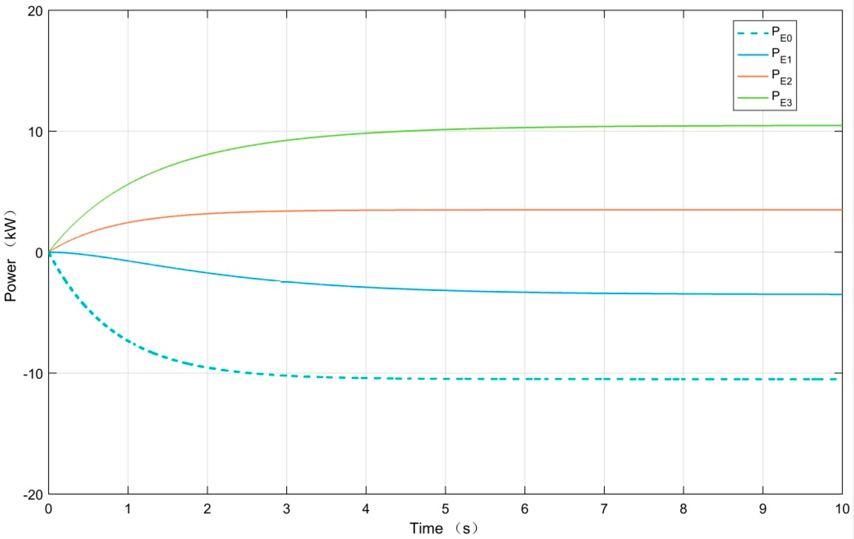
Then power and capacity consensus tracking are both considered. The initial battery storage capacity is $S_{Bat0}=$ 120 kWH, $S_{Bat1}=$ 150 kWH, $S_{Bat2}=$ 180 kWH, $S_{Bat3}=$ 210 kWH. When the system is stable, Figure 9 shows that Module 0 outputs 10.5 kW to microgrid, Module 1 outputs 3.5 kW to microgrid, Module 2 inputs 3.5 kW from microgrid and Module 3 inputs 10.5 kW from microgrid. The distributed battery power in modules is different and $P_{Bat0}=-$10.5 kW, $P_{Bat1}=-$13.5 kW, $P_{Bat2}=-$16.5 kW, $P_{Bat3}=-$19.5 kW as shown in Figure 10. Because the time constant of battery storage capacity is very large, the time to reach power consensus is very long. The difference power among batteries is to eliminate the capacity differences among batteries.

Simulations results show that continuous-time power and capacity consensus tracking is reachable and the leader-following power and capacity consensus tracking model of distributed battery storages in modular microgrid is effective.

6.2. Simulations of Sampled-Data Power Consensus Tracking Strategy

When m = 0, according to Equation (38), the range of the sampling period and sampling delay for system stabilization is:

$$\{\begin{array}{l}0<\tau <0.8\hfill \\ \tau <T<2\tau +1.6\hfill \end{array}$$

(41)

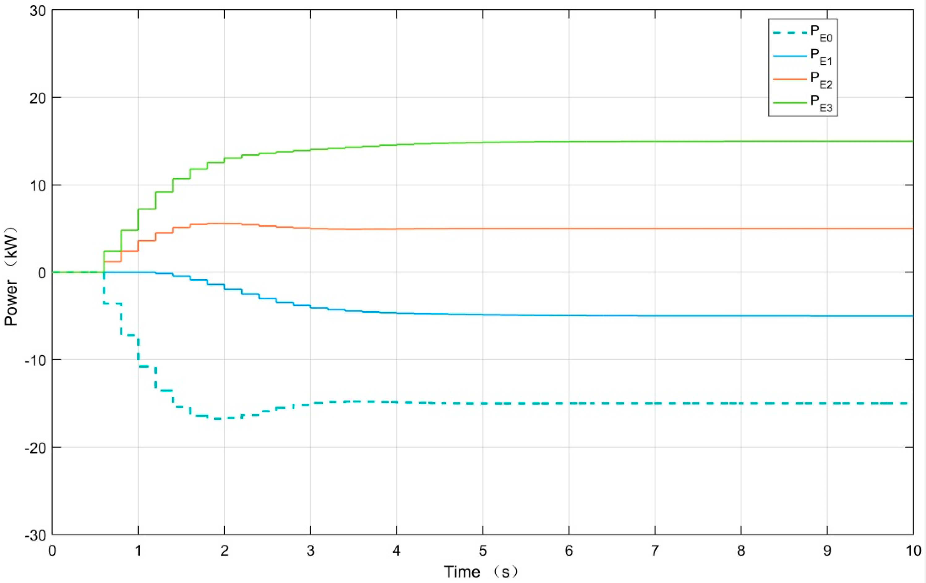
Let the sampling delay $\tau$ = 0.2 s and sampling period T = 0.5 s. Loads are unchanged. Exchange power between each module and microgrid is shown in Figure 11. When the system is stable, module 0 outputs 15 kW to microgrid, module 1 outputs 5 kW to microgrid, module 2 inputs 5 kW from microgrid and module 3 inputs 15 kW from microgrid. The battery power in modules in Figure 12 shows that it tends to be consistent and the discharging power converge to 15 kW after 8 s. Results show that the stabilization range is effective as shown in Equation (41).

When m = 1, according to Equation (39), the range of the sampling period and sampling delay for system stabilization are:

$$\{\begin{array}{l}0<T<0.8\hfill \\ T<\tau <min\left\{2T,T+\frac{\sqrt{1-1.2T}}{1.2}\right\}\hfill \end{array}$$

(42)

Let the sampling period T = 0.2 s and the sampling delay $\tau$ = 0.3 s. Loads are unchanged. Figure 13 shows the exchange power of modules. The battery power in Figure 14 shows that it also realizes the power consensus tracking. But the convergence rate is slower with the decrease of the sampling period. According to Equations (41) and (42), the system is unstable when T = 2.4 s and $\tau$ = 0.2 s. Figure 15 shows that the battery power is divergent.

Simulation results verify the effectiveness of the stable domain of sampling period and sampling delay with sampled-data according to Equation (34).

6.3. Simulations of Sampled-Data Power and Capacity Consensus Tracking Strategy

When sampled-data power and capacity consensus tracking is considered, it is difficult to have the analytical solutions, but easy to have numerical solutions for Equation (40).

Equation (40) is simplified as:

$$F(s)={\displaystyle \prod _{i=1}^3{s}^{2(m+1)}{(s-1)}^2+\frac{Tc}{3600}\left[s^{(m+1)}\epsilon {\lambda }_i+s^{(m+2)}(T-\epsilon ){\lambda }_i\right]+s^{(m+1)}(s-1)\left((T-\epsilon )s+\epsilon \right){\lambda }_i}$$

(43)

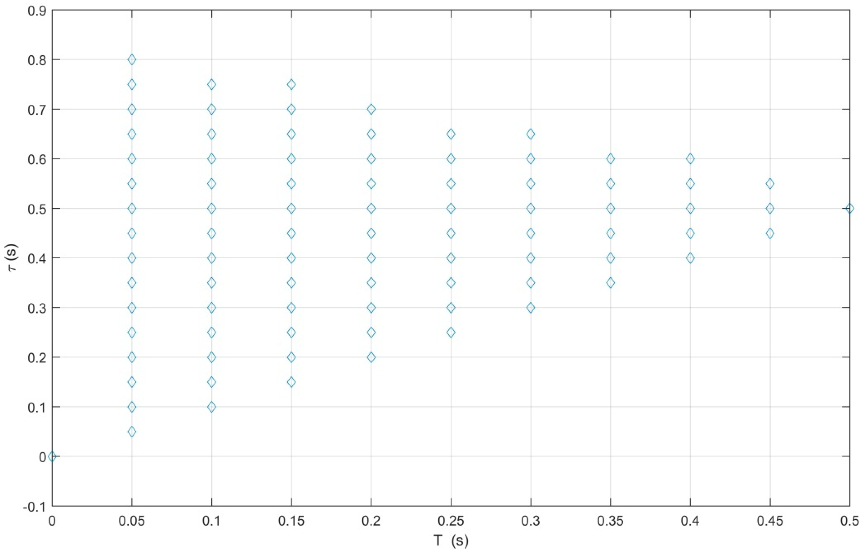
Figure 16 shows the stabilization range of sampling period and sampling delay when m = 0. The stabilization range of sampling period is from 0.1 to 3.2 s. Figure 17 shows the stabilization ranges of sampling period and sampling delay when m = 1. The stabilization range of sampling period is from 0–0.5 s. Figure 18 shows the stabilization ranges of sampling period and sampling delay when m = 2. The stabilization range of sampling period is from 0 to 0.5 s.

The stabilization range of sampling delay varies corresponding to the same sampling period when m is different. The numerical solutions of Equation (43) give a guidance for selection of sampling period and sampling delay to realize the sampled-data bounded power and capacity consensus tracking of distributed battery storages.

6.4. Simulations of Topology Reconfiguration

Figure 19 shows the operation mode of module 3. Grid-connected mode and standalone mode are indicated by 1 and 0 individually. Module 3 is connected to the microgrid from 1 s to 10 s, separated from 10 s to 20 s, and reconnected to the microgrid again from 20 s. Loads in modules remain unchanged. When module 3 is in grid-connected mode, the consensus power is −15 kW. When Module 3 is in standalone mode, the consensus power is −10 kW.

Figure 20 show that all the battery power of modules can realize consensus during the whole process. When Module 3 is off the microgrid, the load of Module 3 is self-supplied and the battery power of Module 3 is −30 kW. Meanwhile, Module 0 outputs 10 kW to microgrid and Module 2 input 10 kW from microgrid as shown in Figure 21.

Simulation results show that the power and capacity consensus tracking strategy of distributed storages is robust under system reconfiguration, which is beneficial to capacity expansion or unexpected exit, and increases the reliability of the system.

6.5. Experiments of Power Consensus Tracking of Distributed Batteries in Modular Microgrid

Figure 22 shows wind power in modules 1, 2 and 3. Wind power varies greatly in the different modules. The average power is 10.08, 12.28, and 12.98 kW, individually. Figure 23 shows solar power in modules 1, 2 and 3. The average power is 5.28, 5.12 and 4.11 kW, individually. The solar power has similar distribution characteristics but there are occasional drops because of partial shadows. Figure 24 shows the load power in different modules. The average power is 19.10, 21.39 and 5.51 kW individually. The load characteristics are also different Because of different electrical uses. If each module runs in standalone mode, the difference between power generation and power consumption is only compensated by the local battery of each module. The battery power is shown as the dotted line A, B, C in Figure 25 and the battery power varies greatly in different module. The drastic fluctuation of battery power damages and reduces the service life of battery, which leads to difficult maintenance of battery. When modules are interconnected and the power and capacity consensus tracking is applied, the consensus battery power is shown as the blue line in Figure 25, which make full use of the space-time complementary power characteristics among modules and greatly decreases the fluctuation of battery power. It shows the consensus power is smoother than stand-alone individual battery power, which can not only prolong the lifespan of batteries, but also realize the unified maintenance of batteries.

7. Conclusions

The power and capacity consensus tracking protocol of distributed battery storage systems in a modular microgrid is designed in this paper. The leader-following power and capacity consensus tracking model of distributed battery storage is established according to the modular microgrid demonstration project on DongAo Island (China). The sufficient and necessary conditions for continuous-time and sampled-data bounded power and capacity consensus tracking of distributed battery storages are deduced by matrix analytical method. The continuous-time power and capacity consensus tracking is stable when the Hermitian matrix of power communication network is positive definite and the ratio of capacity adjacent coefficient to power adjacent coefficient is positive real number. The steady regions of sampling period and sampling delay for sampled-data power and capacity consensus tracking is determined by analytical or numerical solutions. Especially two cases of m = 0 and m = 1 are discussed in detail. Simulation results verify the validation of the power and capacity consensus tracking strategy and the stabilization ranges of parameters. The power and capacity consensus tracking is robust under reconfiguration of the modular microgrid. Experiments on a wind-solar modular microgrid show that the power and capacity consensus tracking of distributed storages makes full use of the space-time complementary power characteristics among modules, improving the lifespan and realizing the unified maintenance of batteries. The power and capacity consensus tracking strategy determine the exchange power among modules. Therefore the control problem of modular microgrid is solved completely and the economic promotion of modular microgrids is realized.

References

- Mumtaz, F.; Bayram, I.S. Planning, operation, and protection of microgrids: An overview. Energy Procedia 2017, 107, 94–100. [Google Scholar] [CrossRef]
- Wang, J.; Zhong, H.; Tang, W.; Rajagopal, R.; Xia, Q.; Kang, C.; Wang, Y. Optimal bidding strategy for microgrids in joint energy and ancillary service markets considering flexible ramping products. Appl. Energy 2017, 205, 294–303. [Google Scholar] [CrossRef]
- Chmiel, Z.; Bhattacharyya, S.C. Analysis of off-grid electricity system at Isle of Eigg (Scotland): Lessons for developing countries. Renew. Energy 2015, 81, 578–588. [Google Scholar] [CrossRef] [Green Version]
- Panora, R.; Gehret, J.E.; Furse, M.M.; Lasseter, R.H. Real-world performance of a CERTS microgrid in Manhattan. IEEE Trans. Sustain. Energy 2013, 5, 1356–1360. [Google Scholar] [CrossRef]
- Chen, C.; Chen, J.; Cao, H.; Huang, Y.; Xiao, Y.; Li, L. Control scheme of bi-directional converter for microgrid under the model of parallel running on Nanji island. IEEE Trans. Smart Grid 2014, 2, 30–36, (In Chinese with English abstract). [Google Scholar]
- Marzband, M.; Fouladfar, M.H.; Akorede, M.H.; Lightbody, G.; Pouresmaeil, E. Framework for smart transactive energy in home-microgrids considering coalition formation and demand side management. Sustain. Cities Soc. 2018, 40, 136–154. [Google Scholar] [CrossRef]
- Marzband, M.; Fouladfar, M.H.; Savaghebi, M.; Pouresmaeil, E.M.; Guerrero, J.; Lightbody, G. Smart transactive energy framework in grid-connected multiple home microgrids under independent and coalition operations. Renew. Energy 2018, 126, 95–106. [Google Scholar] [CrossRef]
- Marzband, M.; Sumper, A.; Ruiz-Alvarez, A.; Dominguez-Garcia, J.L.; Tomoiaga, B. Experimental evaluation of a real time energy management system for stand-alone microgrids in day-ahead markets. Appl. Energy 2013, 106, 365–376. [Google Scholar] [CrossRef]
- Turner, G.; Kelley, J.P.; Storm, C.L.; Wetz, D.A.; Lee, W.L. Design and active control of a microgrid testbed. IEEE Trans. Smart Grid 2017, 6, 73–81. [Google Scholar] [CrossRef]
- Stadler, M.; Cardoso, G.; Mashayekh, S.; Forget, T.; Deforest, N.; Agarwal, A.; Schönbein, A. Value streams in microgrids: A literature review. Appl. Energy 2016, 162, 980–989. [Google Scholar] [CrossRef] [Green Version]
- Bevrani, H.; Shokoohi, S. An intelligent droop control for simultaneous voltage and frequency regulation in islanded microgrids. IEEE Trans. Smart Grid 2013, 4, 1505–1513. [Google Scholar] [CrossRef]
- Ribeiro, L.A.D.S.; Saavedra, O.R.; Lima, S.L.D.; Matos, J.G.D. Isolated micro-grids with renewable hybrid generation: The case of Lençóis Island. IEEE Trans. Sustain. Energy 2010, 2, 1–11. [Google Scholar] [CrossRef]
- Alegria, E.; Brown, T.; Minear, E.; Lasseter, R.H. CERTS microgrid demonstration with large-scale energy storage and renewable generation. IEEE Trans. Smart Grid 2014, 5, 937–943. [Google Scholar] [CrossRef]
- Cagnano, A.; De Tuglie, E.; Dicorato, M.; Forte, G.; Trovato, M. PrinCE Lab experimental microgrid Planning and operation issues. In Proceedings of the 2015 IEEE 15th International Conference on Environment and Electrical Engineering (EEEIC), Rome, Italy, 10–13 June 2015; pp. 1671–1676. [Google Scholar] [CrossRef]
- Cagnano, A.; De Tuglie, E.; Cicognani, L. Prince-Electrical Energy Systems Lab: A pilot project for smart microgrids. Electr. Power Syst. Res. 2017, 148, 10–17. [Google Scholar] [CrossRef]
- Guerrero, J.M.; Vasquez, J.C.; Matas, J.; Vicuna, L.G.D.; Castilla, M. Hierarchical control of droop-controlled AC and DC microgrids—A general approach toward standardization. IEEE Trans. Ind. Electron. 2011, 58, 158–172. [Google Scholar] [CrossRef]
- Bidram, A.; Davoudi, A. Hierarchical structure of microgrids control system. IEEE Trans. Smart Grid 2012, 3, 1963–1976. [Google Scholar] [CrossRef]
- Riverso, S.; Tucci, M.; Vasquez, J.C.; Guerrero, J.M.; Ferrari-Trecate, G. Stabilizing plug-and-play regulators and secondary coordinated control for AC islanded microgrids with bus-connected topology. Appl. Energy 2018, 210, 655–661. [Google Scholar] [CrossRef]
- Godina, M.; Rodrigues, E.M.G.; Pouresmaeil, E.; Matias, J.C.O.; Catalao, J.P.S. Model predictive control home energy management and optimization strategy with demand response. Appl. Sci. 2018, 8, 408. [Google Scholar] [CrossRef]
- Godina, R.; Rodrigues, E.M.G.; Pouresmaeil, E.; Catalao, J.P.S. Optimal residential model predictive control energy management performance with PV microgeneration. Comput. Oper. Res. 2017, 1–14. [Google Scholar] [CrossRef]
- Tavakoli, M.; Shokridehaki, F.; Akorede, M.F.; Marzband, M.; Vechiu, I.; Pouresmaeil, E. CVaR-based energy management scheme for optimal resilience and operational cost in commercial building microgrids. Int. J. Electr. Power Energy Syst. 2018, 100, 1–9. [Google Scholar] [CrossRef]
- Shuai, H.; Fang, J.; Ai, X.; Tang, Y.; Wen, J.; He, H. Stochastic optimization of economic dispatch for microgrid based on approximate dynamic programming. IEEE Trans. Smart Grid 2018, 1. [Google Scholar] [CrossRef]
- Wang, S.; Peng, D.; Dong, R.; Yong-He, L. Modified Flower Pollination Algorithm and Applications on Optimization Dispatch of Microgrid. J. Northeast. Univ. 2018, 39, 334–338, (In Chinese with English abstract). [Google Scholar] [CrossRef]
- Kerdphol, T.; Fuji, K.; Mitani, Y.; Watanabe, M.; Qudaih, Y. Optimization of a battery energy storage system using particle swarm optimization for stand-alone microgrids. Int. J. Electr. Power Energy Syst. 2016, 81, 32–39. [Google Scholar] [CrossRef]
- Zhang, X.; Yeh, W.; Jiang, Y.; Huang, Y.; Xiao, Y.; Li, L. A case study of control and improved simplified swarm optimization for economic dispatch of a stand-alone modular microgrid. Energies 2018, 11, 793. [Google Scholar] [CrossRef]
- Zhang, X.; Shu, J.; Wu, C.; Zhou, L.; Song, X. Island microgrid based on distributed photovoltaic generation. Power Syst. Prot. Control 2014, 6, 55–61, (In Chinese with English abstract). [Google Scholar] [CrossRef]
- Zhou, L.; Shu, J.; Zhang, X.; Zhang, Z. Control strategy of voltage quality in distributed energy microgrids. Power Syst. Technol. 2012, 36, 18–22, (In Chinese with English abstract). [Google Scholar] [CrossRef]
- Zhang, X.; Zhang, X.; Li, L.; Luo, F.; Zhang, Y. A new cascaded control strategy for paralleled line-interactive UPS with LCL filter. Earth Environ. Sci. 2016, 40. [Google Scholar] [CrossRef]
- Dufo-López, R.; Bernal-Agustín, J.L. Multi-objective design of pv–wind–diesel–hydrogen–battery systems. Renew. Energy 2008, 33, 2559–2572. [Google Scholar] [CrossRef]
- Jenkins, D.P.; Fletcher, J.; Kane, D. Lifetime prediction and sizing of lead-acid batteries for microgeneration storage applications. IET Renew. Power Gener. 2008, 2, 191–200. [Google Scholar] [CrossRef]
- Fotouhi, A.; Propp, K.; Auger, D.J.; Longo, S. State of Charge and State of Health Estimation Over the Battery Lifespan. Green Energy Technol. 2018, 267–288. [Google Scholar] [CrossRef]
- Zhang, X.; Yu, T.; Yang, B.; Li, L. Virtual generation tribe based robust collaborative consensus algorithm for dynamic generation command dispatch optimization of smart grid. Energy 2016, 101, 34–51. [Google Scholar] [CrossRef]
- Miloje, S.R.; Miroslav, K. Distributed adaptive consensus and synchronization in complex networks of dynamical systems. Automatica 2018, 91, 233–243. [Google Scholar] [CrossRef]
- Zhang, Z.; Chow, M.-Y. Incremental cost consensus algorithm in a smart grid environment. In Proceedings of the Power and Energy Society General Meeting, San Diego, CA, USA, 24–29 July 2011; Volume 5, pp. 1–6. [Google Scholar] [CrossRef]
- Zhang, Z.; Chow, M.-Y. Convergence analysis of the incremental cost consensus algorithm under different communication network topologies in a smart grid. IEEE Trans. Power Syst. 2012, 27, 1761–1768. [Google Scholar] [CrossRef]
- Han, R.; Meng, L.; Trecate, G.F.; Coelho, E.A.A.; Vasquez, J.C.; Guerrero, J.M. Containment and consensus-based distributed coordination control for voltage bound and reactive power sharing in AC microgrid. In Proceedings of the Applied Power Electronics Conference and Exposition (APEC), Tampa, FL, USA, 26–30 March 2017; Volume 6, pp. 3549–3566. [Google Scholar] [CrossRef]
- Li, L.; Zhang, X.; Wang, Z.; Lin, Z. Consensus of Leader-Following Multi-Agent Systems with Sampling Information under Directed Networks. In Proceedings of the IEEE International Conference on CSE & EUC, Guangzhou, China, 21–24 July 2017; Volume 10, pp. 63–68. [Google Scholar] [CrossRef]
- Li, L.; Fang, H. Bounded consensus of leader-following multi-agent systems with sampling delay for double-integrator dynamics. Int. J. Model. Identif. Control 2013, 19, 323–332. [Google Scholar] [CrossRef]
- Shi, Y.; Yin, Y.; Wang, S.; Liu, Y.; Liu, F. Distributed Leader-following Consensus of Nonlinear Multi-agent Systems with Nonlinear Input Dynamics. Neurocomputing 2018, 286, 193–197. [Google Scholar] [CrossRef]
- Ren, W. Multi-vehicle consensus with a time-varying reference state. Syst. Control Lett. 2007, 56, 474–483. [Google Scholar] [CrossRef]
- Hu, J.; Hong, Y. Leader-following coordination of multi-agent systems with coupling time delays. Physica A 2007, 374, 853–863. [Google Scholar] [CrossRef] [Green Version]
- Ren, W.; Cao, Y. Convergence of sampled-data consensus algorithms for double-integrator dynamics. In Proceedings of the 47th IEEE Conference on Decision and Control, Cancun, Mexico, 9–11 December 2008; Volume 16, pp. 3965–3970. [Google Scholar] [CrossRef]
Figure 1.
Modular microgrid on DongAo Island.
Figure 2.
Structure of modular microgrid on DongAo Island.
Figure 3.
Topology of the three-port converter.
Figure 4.
Power flow chart of the modular microgrid.
Figure 5.
Undirected communication network of leader-following multi-agent systems.
Figure 6.
Undirected communication network of modular microgrid.
Figure 7.
Exchange power of modules.
Figure 8.
Battery power in modules.
Figure 9.
Figure 10.
Figure 11.
Exchange power of modules (, T = 0.5 s).
Figure 12.
Battery power in modules (, T = 0.5 s).
Figure 13.
Exchange power of modules (, T = 0.2 s).
Figure 14.
Battery power in modules (, T = 0.2 s).
Figure 15.
Battery power in modules (, T = 2.4 s).
Figure 16.
Stabilization ranges of sampling period and sampling delay ().
Figure 17.
Figure 18.
Figure 19.
Operation state of module D.
Figure 20.
Exchange power in modules.
Figure 21.
Figure 22.
Wind power.
Figure 23.
Solar power.
Figure 24.
Load power.
Figure 25.
Battery power.
© 2018 by the authors. Licensee MDPI, Basel, Switzerland. This article is an open access article distributed under the terms and conditions of the Creative Commons Attribution (CC BY) license (http://creativecommons.org/licenses/by/4.0/).
Share and Cite
MDPI and ACS Style
Zhang, X.; Huang, Y.; Li, L.; Yeh, W.-C. Power and Capacity Consensus Tracking of Distributed Battery Storage Systems in Modular Microgrids. Energies 2018, 11, 1439. https://doi.org/10.3390/en11061439
AMA Style
Zhang X, Huang Y, Li L, Yeh W-C. Power and Capacity Consensus Tracking of Distributed Battery Storage Systems in Modular Microgrids. Energies. 2018; 11(6):1439. https://doi.org/10.3390/en11061439
Chicago/Turabian StyleZhang, Xianyong, Yaohong Huang, Li Li, and Wei-Chang Yeh. 2018. "Power and Capacity Consensus Tracking of Distributed Battery Storage Systems in Modular Microgrids" Energies 11, no. 6: 1439. https://doi.org/10.3390/en11061439
Note that from the first issue of 2016, this journal uses article numbers instead of page numbers. See further details here.