1. Introduction
During the last decade, and due to aspects such as climate change, energy dependence, fossil resource scarcity and the increasing costs of nuclear power [
1], most developed countries have promoted large-scale integration of Renewable Energy Sources (RES), mainly wind and PV power plants [
2]. This relevant integration of RES has raised important concerns in terms of grid stability and reliability, mainly due to: (i) the nature of RES power variation [
3] as well as the uncertainty in the privately-owned renewable generators that puts the generation-load balance at risk [
4]; (ii) the reduction of the total system inertia by the decoupling between rotor mechanical speed and grid frequency [
5], or even the absence of rotating machines [
6]. As the system inertia decreases, an increase of primary frequency control (PFC) reserves is needed [
7]. Traditionally, PFC reserves are provided by synchronous generators [
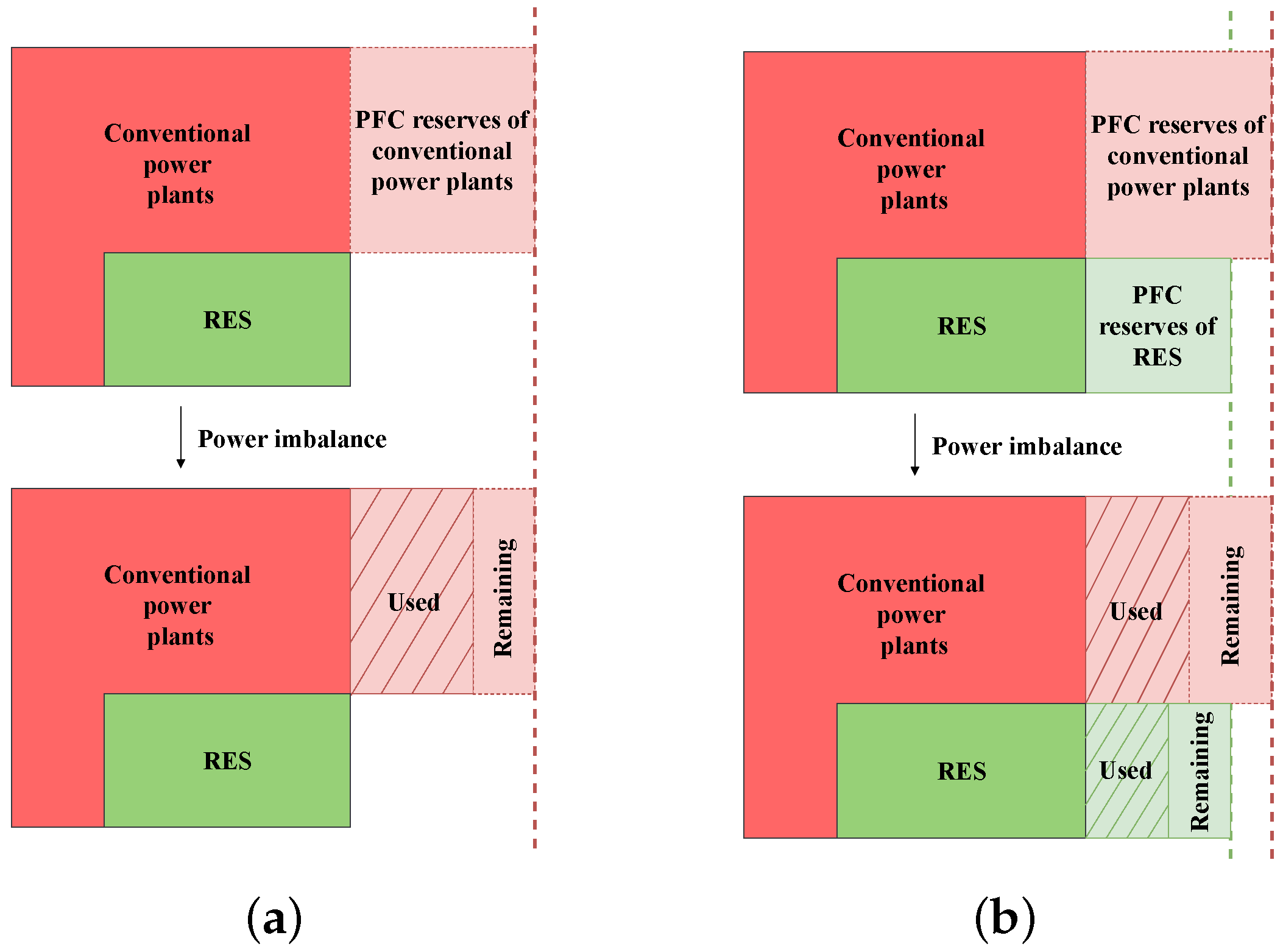
8], as depicted in
Figure 1a. Under power imbalance conditions, PFC reserves from conventional generation are traditionally released to compensate the disturbance and recover the rate grid frequency. If these reserves cannot compensate for the mismatch, it could cause a sharp decrease of the system frequency [
9]. With the relevant penetration of wind power plants, some proportional capacity of the system reserves must be provided by them [
7,
10] see
Figure 1b. Additional reserves can be then provided by renewables, reducing the primary reserves from conventional generation units and providing enhanced solutions for weak and/or isolated power systems [
9,
11]. Under this scenario of high RES penetration, transmission system operators have required that not only conventional utilities contribute to ancillary services [
12], but also renewables, especially wind power plants [
13]. Indeed, [
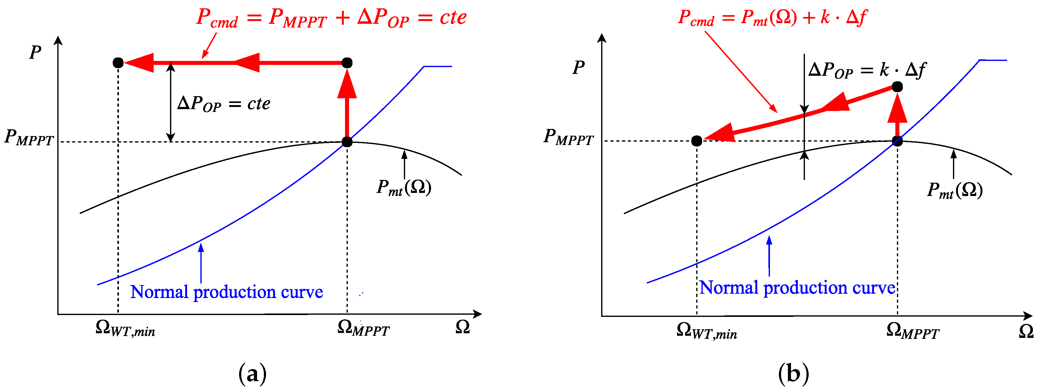
14] affirms that the participation of the wind power plants in the ancillary services such as grid frequency control becomes inevitable. For this reason, frequency control strategies are being developed to effectively integrate Variable Speed Wind Turbines (VSWTs) into the grid, in order to replace conventional power plants by maintaining a secure power system operation [
15]. Most of them are based on ‘hidden inertia emulation’, in order to enhance the inertia response of VSWTs [
16,
17]. A classification for different control strategies based on principles for inertia emulation concept can be found in [
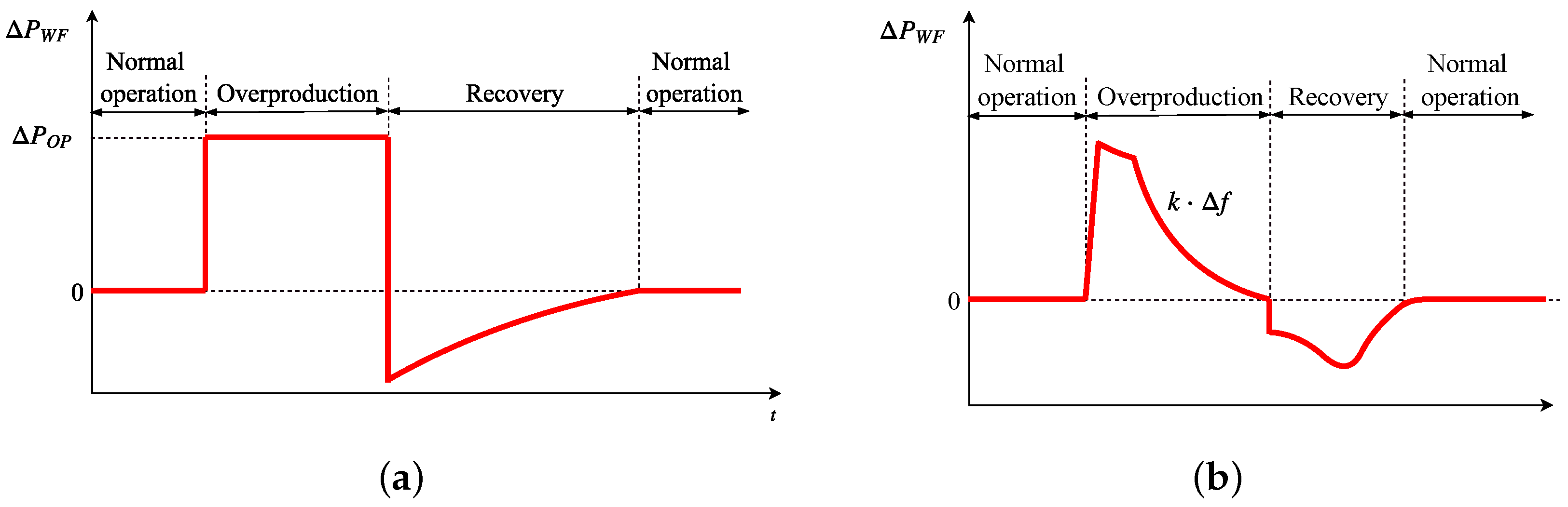
18]. One of the possible solutions to overcome this is called fast power reserve emulation. It is based on supplying the kinetic energy stored in the rotating masses to the grid as an additional active power, being afterwards recovered through an under-production period (recovery). Overproduction is defined in the specific literature over the electrical pre-event power reference [
19,
20,
21,
22,
23,
24] and the overproduction power is considered as constant and independent from the frequency excursion severity [
21,
22,
23]. Other proposals define the time that the wind power plant must be overproducing independently from the event [
19,
20,
21,
22] or consider that it should last until the wind turbine achieves its minimum speed limit [
23]. Moreover, the transition from overproduction to recovery is defined as an abrupt drop in the active generated power by VSWTs [
21,
23,
24] or as a constant slope [
19,
22]. A different strategy is described in [
20], where the VSWTs of the wind power plant are designed to recover at different times, avoiding ‘synchronization’. Most contributions consider a low wind energy integration for simulations, between 10 and 20% [
19,
20,
22], and only recent contributions analyze penetration level scenarios up to 40% [
10]. However, the renewable share is currently over 20% in different power systems. Actually, some countries have already experienced instantaneous penetration higher than 50% (i.e., Spain, Portugal, Ireland, Germany and Denmark) [
25]. Subsequently, scenarios with a very relevant integration of wind energy should be considered and evaluated.
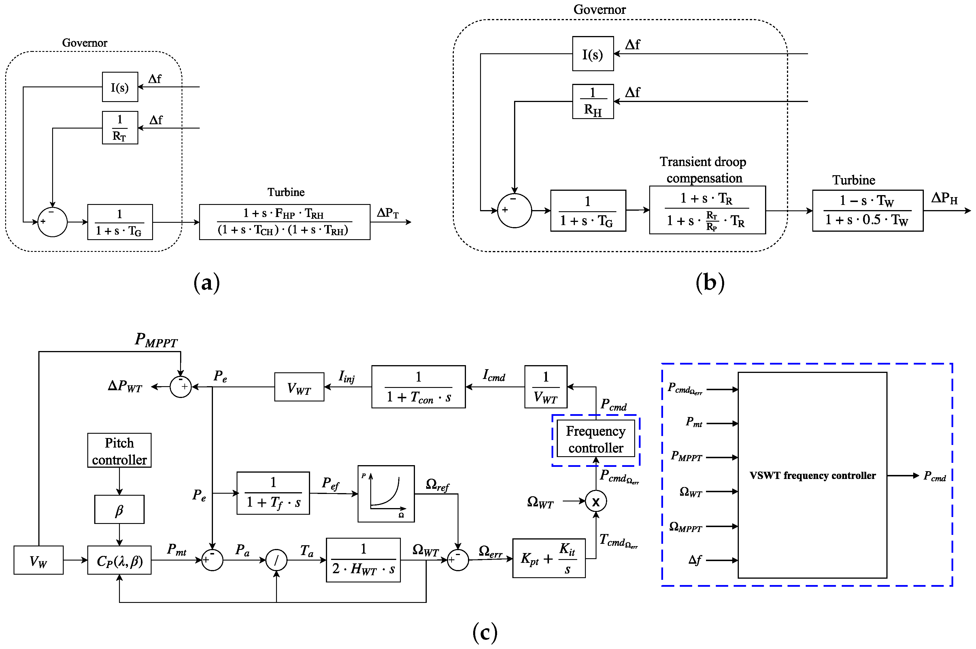
To overcome these drawbacks, and with the aim of improving the frequency response of power systems with massive wind energy penetration, this paper describes and evaluates an alternative fast power reserve emulation controller. The main contributions of this paper are summarized as follows:
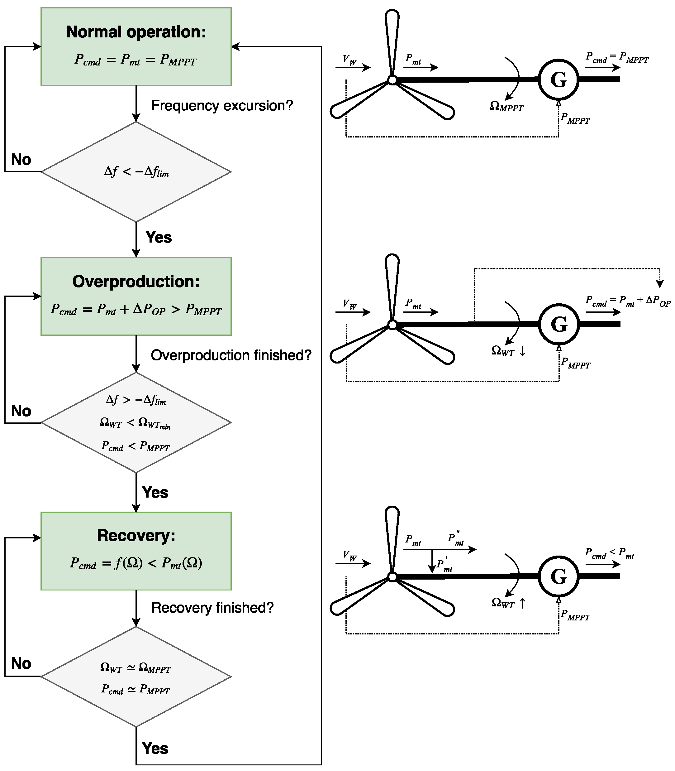
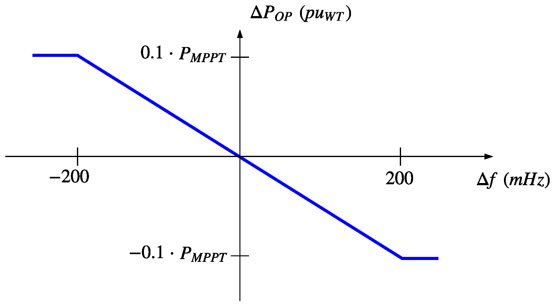
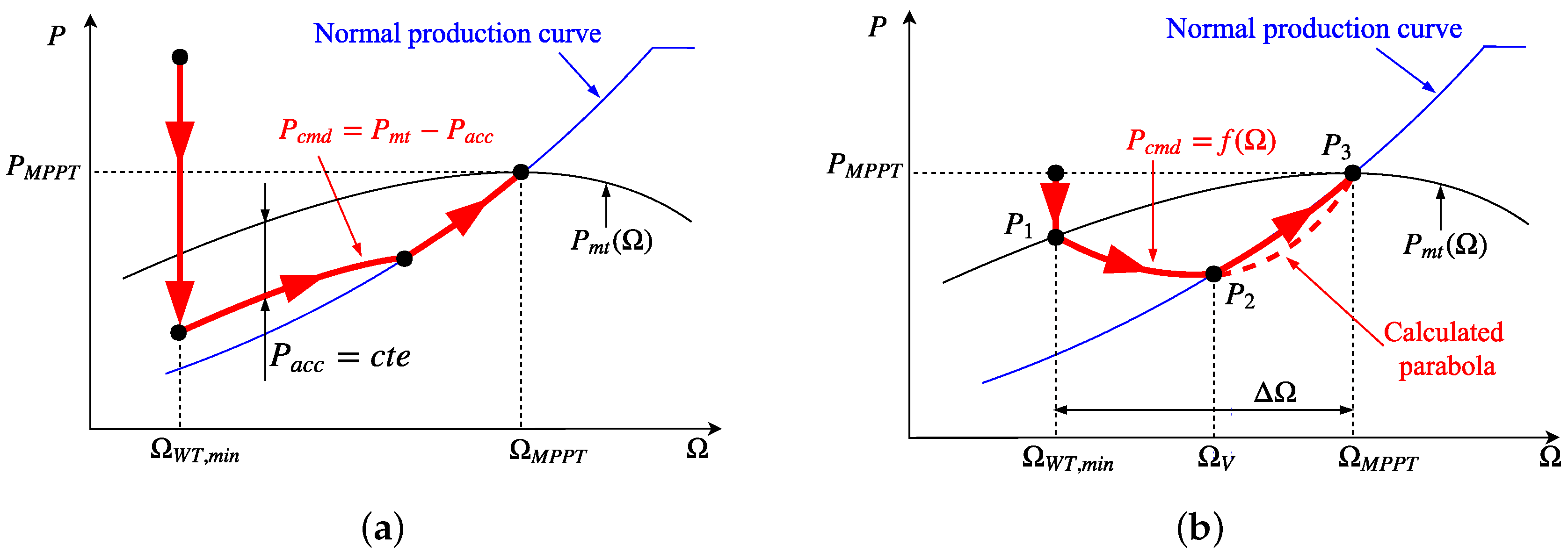
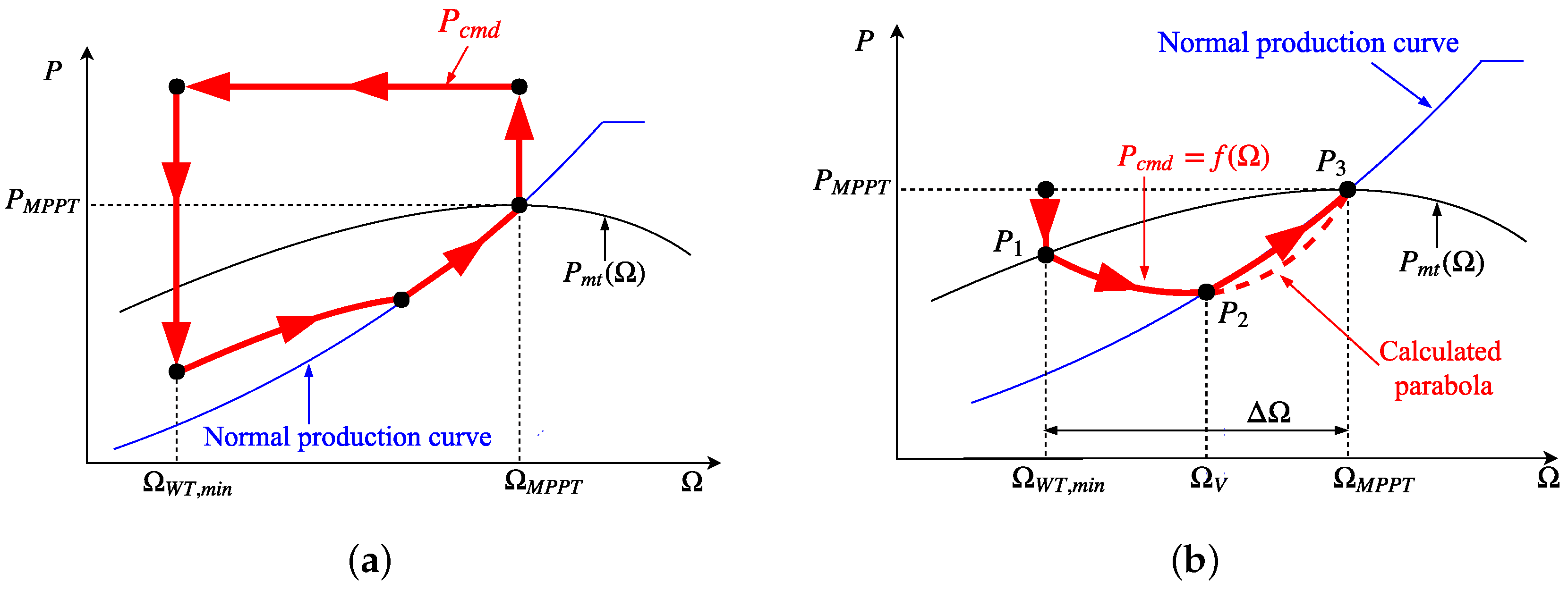
The active power provided by VSWTs during the overproduction operation mode is defined over the mechanical power instead of the pre-event electrical power. Such mechanical power varies with the rotational speed instead of keeping constant as the former one. Moreover, the overproduction power is estimated according to the frequency excursion, being thus an ‘adaptive’ overproduction strategy.
The active power provided by VSWTs during the recovery operation mode is defined below the mechanical power to recover the rotational energy delivered in the overproduction mode. It is defined as a parabolic trajectory until the rotational speed reaches the maximum power tracking curve. Thereafter, that curve is followed. Because of that, it is considered as a ‘smooth’ recovery period.
The control strategy proposed has been tested under different scenarios, considering a maximum wind energy integration of 45%. In all the scenarios, the proposed solution reduces significantly the grid frequency deviations under power imbalance conditions.
The rest of the paper is organized as follows: in
Section 2 the proposed frequency controller for VSWTs is described and compared to previous approaches. The power system and the different scenarios needed to assess the proposed control are discussed in
Section 3. Simulation results are given in
Section 4. Finally,
Section 5 gives the conclusions.
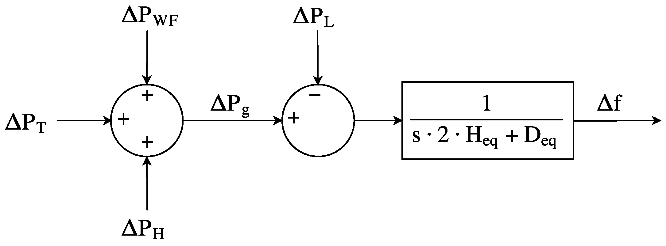
4. Results
With the aim of evaluating the suitability of the proposed VSWTs frequency controller, three different strategies have been analyzed:
Thermal and hydro-power plants with frequency control (without frequency response from wind power plants).
Thermal and hydro-power plants with frequency control and wind power plants with the frequency controller of [
23].
Thermal and hydro-power plants with frequency control and wind power plants with the proposed frequency controller.
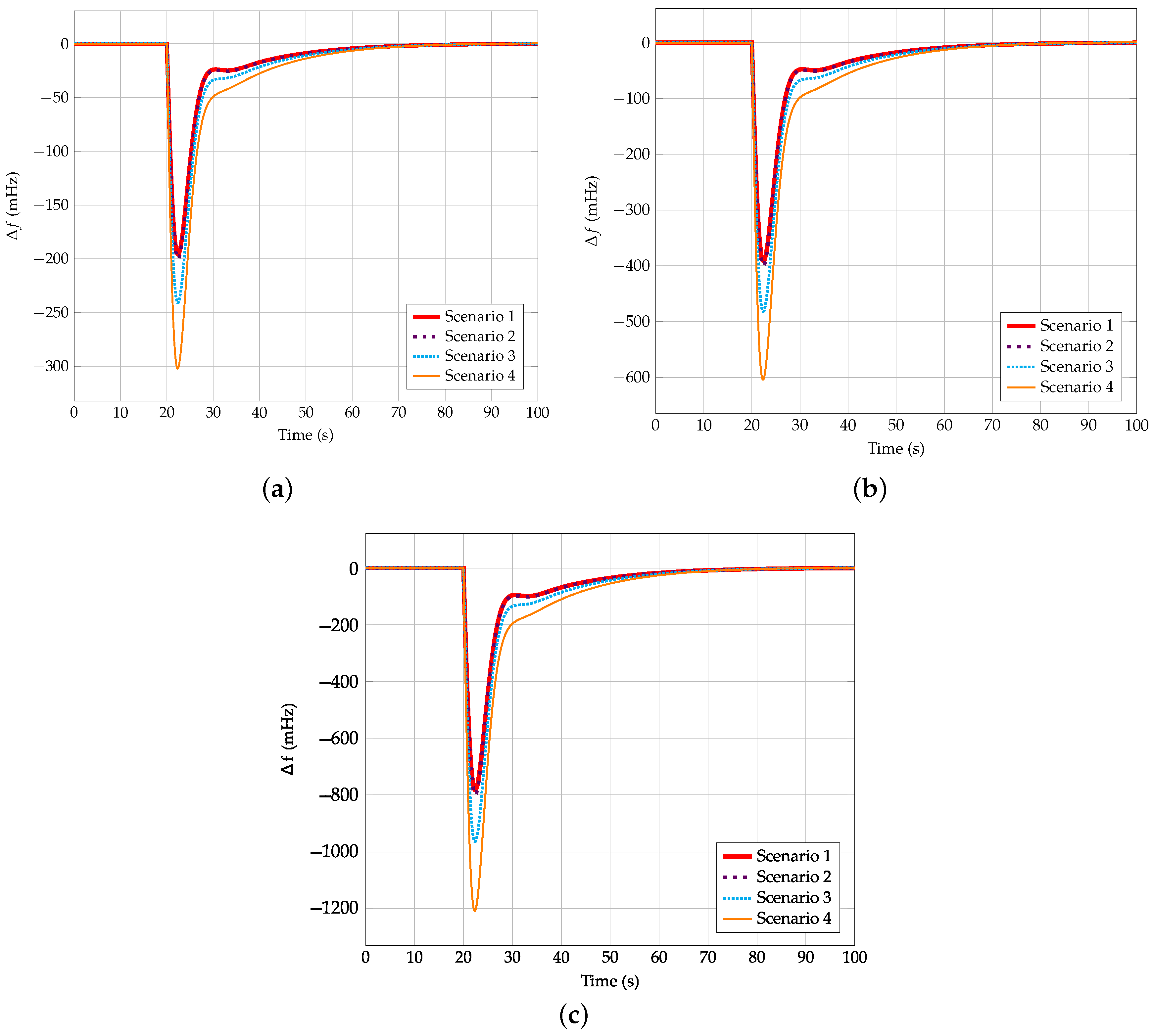
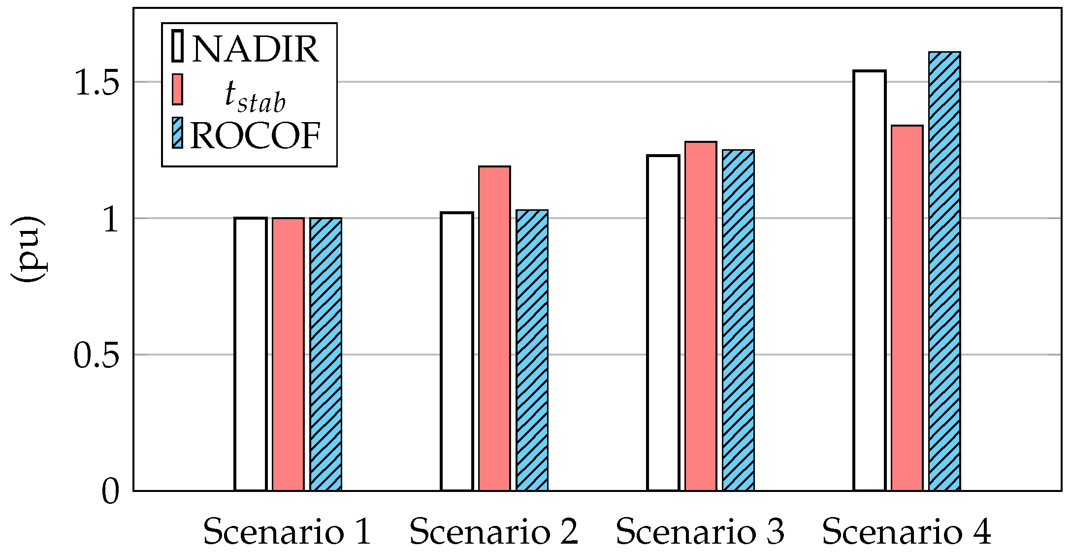
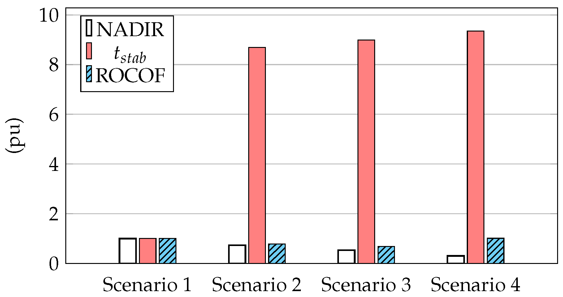
When wind power plants are excluded from frequency control, frequency excursions by considering the different scenarios are shown in
Figure 12. As wind power integration increases, without providing frequency response, the lowest point or Nadir becomes more and more significant, achieving
mHz in scenario 4 considering the same value of
, being over
times in comparison to the first one. With regard to the stabilization time (defined as the time interval taken by the frequency deviation to be within the range
mHz [
32]), it enhances slightly. In scenario 4, it is
times over the first one, increasing from 28 to 34 s. The rate of change of frequency (ROCOF) also increases with the integration of wind energy without frequency response, from 83 mHz/s in scenario 1 to 132 mHz/s in scenario 4. Therefore, the more wind power integration into grids, the more sensitive is the power system under imbalance conditions. Subsequently, a more unstable grid results from the integration of renewables without implementing any frequency response. Similar relationships are found when
and
(
Figure 12b,c, respectively). In
Figure 13, a comparison among Nadir, stabilization time and ROCOF for the different scenarios and
is depicted. Results are shown in pu, considering as base the results of scenario 1, where there are no wind power plants.
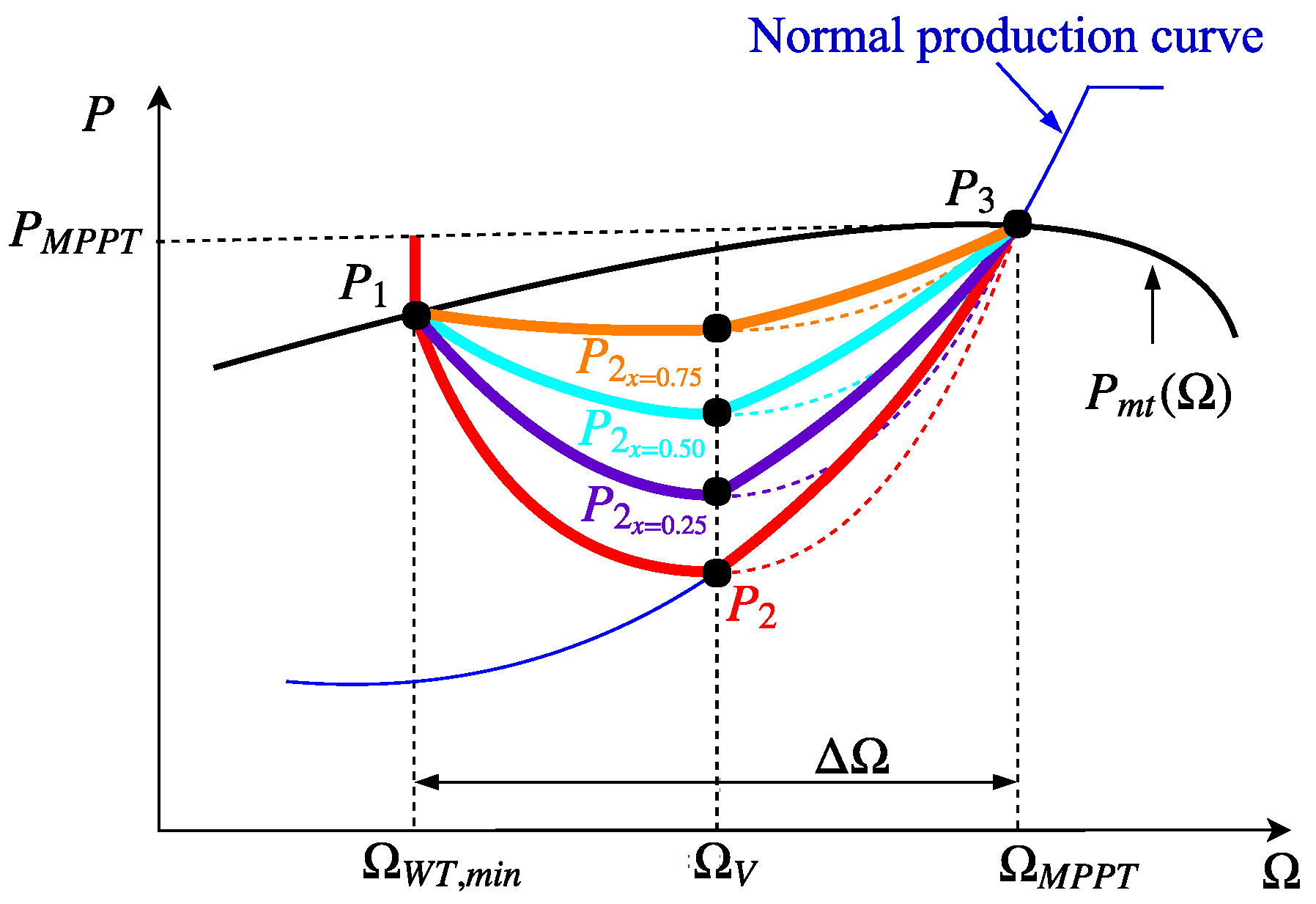
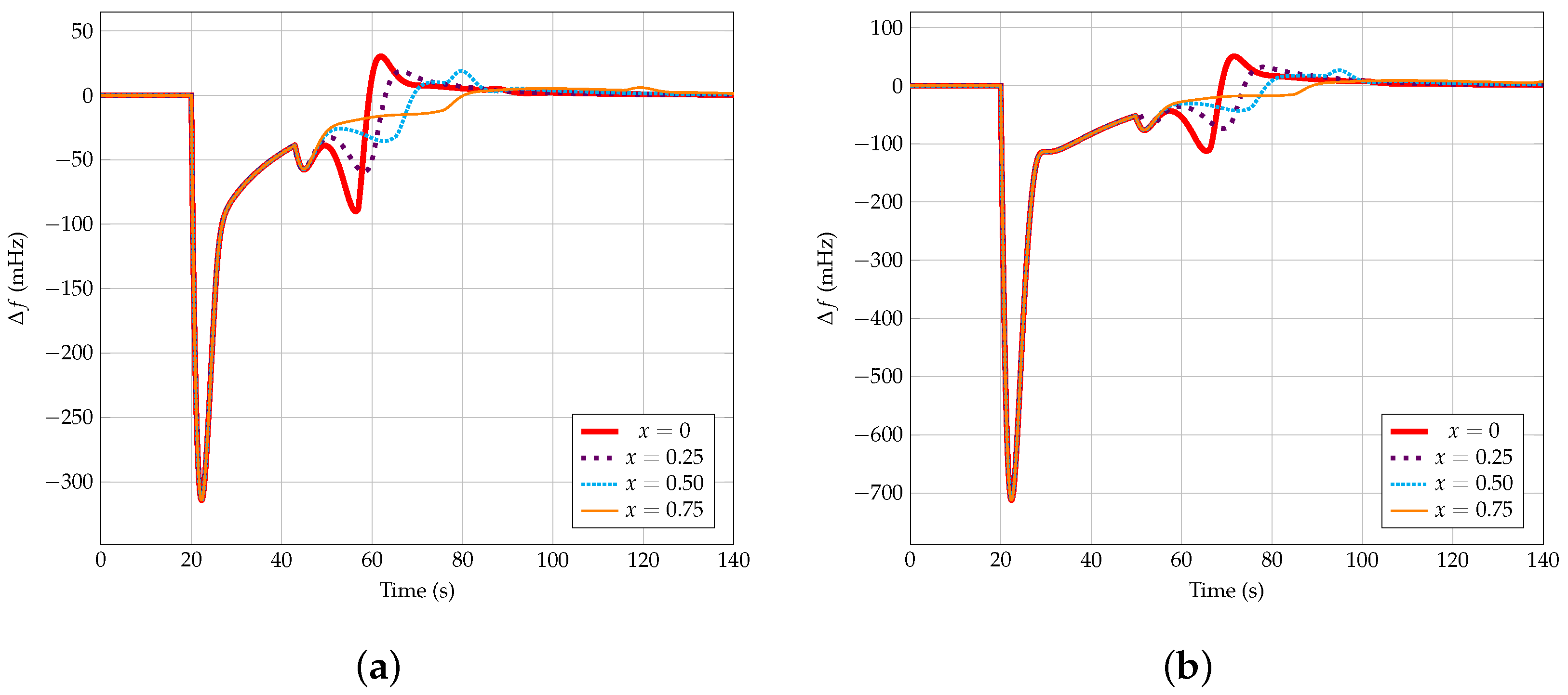
To overcome previous frequency excursion drawbacks, and to determine the most suitable recovery strategy of the smooth controller proposed in this work, the four different recovery strategies are analyzed hereinafter. They are represented for the scenario 2, considering
in
Figure 14a and
in
Figure 14b. Due to the low value of the power of point
(see
Figure 7), the frequency deviation presents undesirable oscillations when the wind power plant is within the recovery operation mode. This effect is especially significant in the original proposal, and it is reduced as the power considers the difference between the actual mechanical power
and the maximum mechanical power available according to the wind speed
. Actually, the best response is obtained when
is defined as
. Because of that, the rest of the results only consider that case (
).
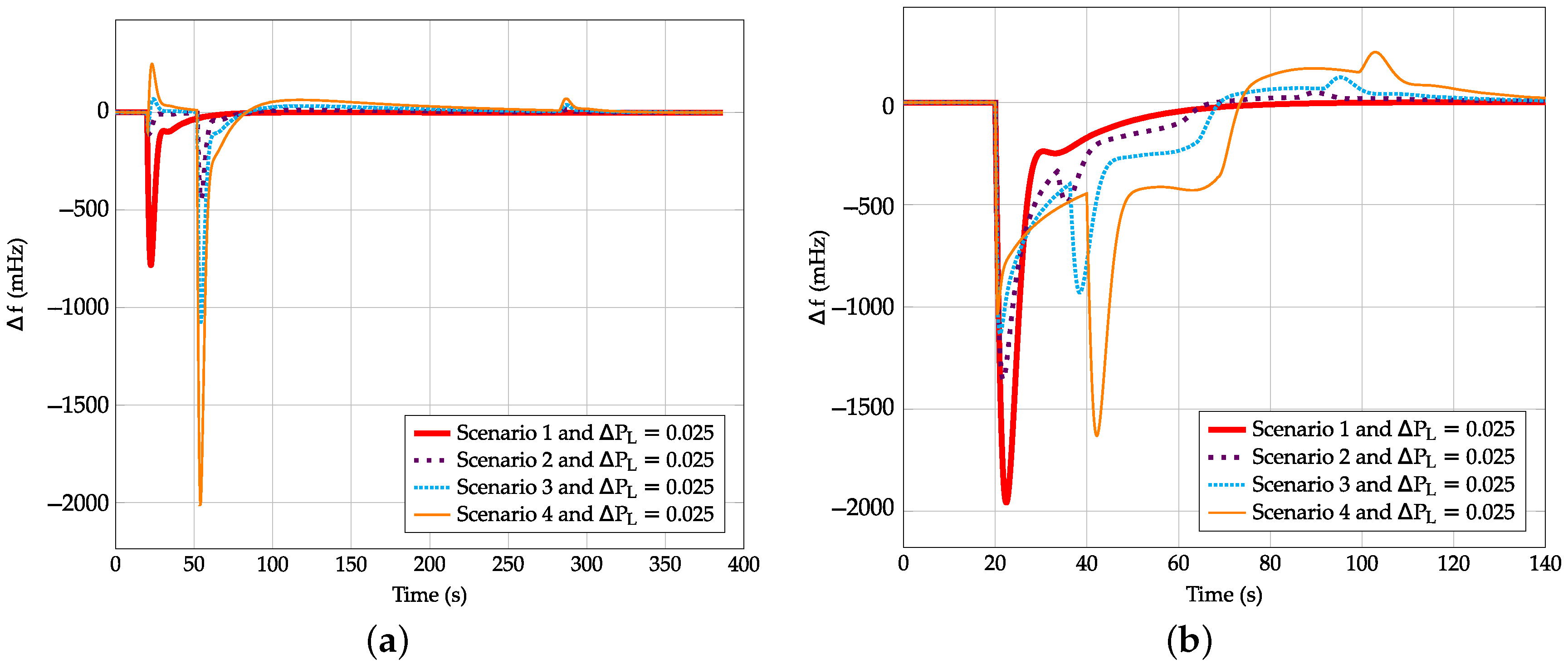
Figure 15,
Figure 16 and
Figure 17 summarize the different scenarios including frequency response from VSWTs when
,
and
, respectively.
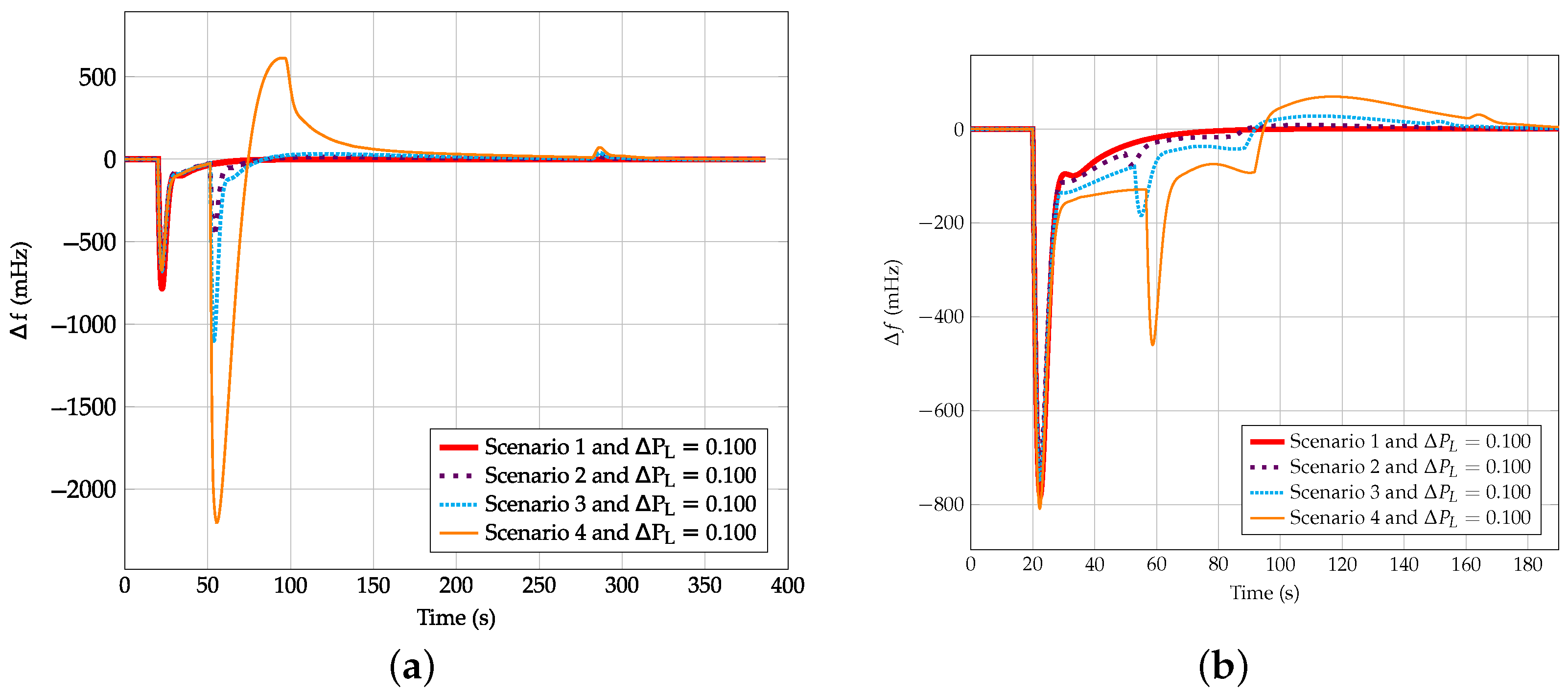
Figure 15a,
Figure 16a and
Figure 17a refer to the controller indicated in [
23].
Figure 15b,
Figure 16b and
Figure 17b use the new proposal of this work, assuming
in line with the previous discussion. According to the results, scenarios 2–4 present two different well-identified frequency shifts: (i) due to the power imbalance and (ii) due to the supply-side decrease as a consequence of the step from overproduction to recovery operation mode of the VSWTs frequency controller, see
Figure 8.
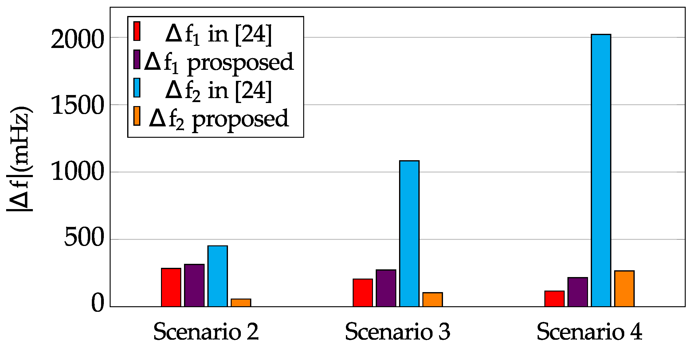
With regard to the power imbalance condition, the frequency shift decreases as the wind energy integration increases. This reduction is due to the fast support provided by VSWTs under a generation-load mismatch. It is more noticeable when the proposal of [
23] is considered, as the overproduction power is constant and independent from the frequency deviation. Actually, if the demand variation is small (i.e.,
), the overproduction mode of the approach indicated in [
23] may cause an overfrequency instead of an underfrequency, since the additional active power definition
(see
Figure 15a, scenarios 3 and 4). This drawback does not occur if the adaptive frequency controller proposed in this work is used, as seen in
Figure 15b. Considering the case in which
, a reduction of 70% is obtained with the approach of [
23], from 391 mHz in the first scenario to 117 in the last one. This reduction accounts for the 44%, reaching 215 mHz in scenario 4 with the new controller proposal. Finally, when
, both frequency controllers have similar responses during the firsts seconds, reaching a Nadir
mHz.
With respect to the second frequency shift, it increases with high wind power plant integration, as it increase leads to a greater wind power generation reduction when switching from overproduction to recovery. The underfrequency value can decrease to 2 Hz in scenario 4 with the approach indicated in [
23], due to the sudden drop of generation from VSWTs, see
Figure 9. Nevertheless, this second excursion is reduced using the smooth recovery proposal of this work, decreasing up to 163, 266, 450 mHz for scenario 4 when
,
,
, respectively. This fact brings out that the new proposed adaptive and smoother controller gives an improvement of the frequency response, being suitable for power systems with high wind power penetration. In
Figure 18, a comparison between both frequency deviations corresponding to both frequency control strategies considering
are depicted.
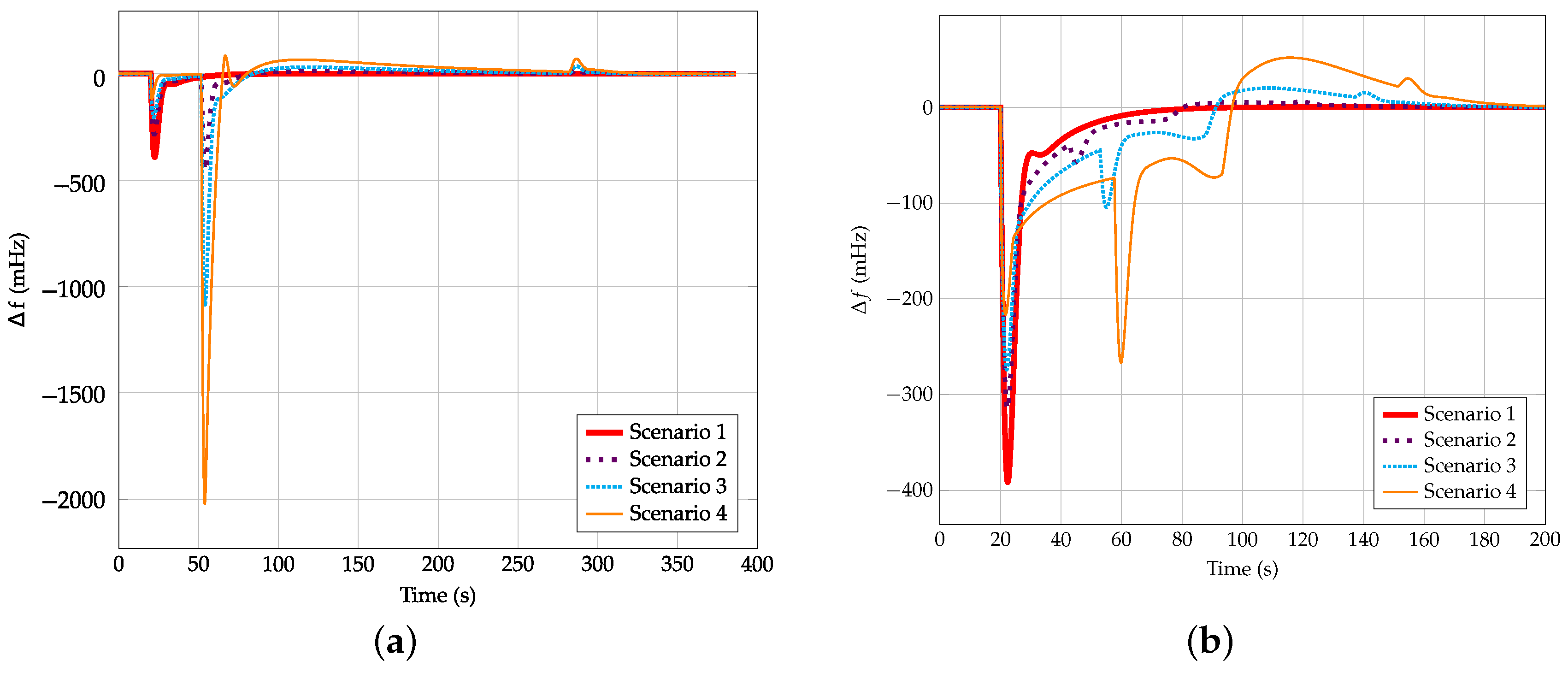
Regarding to ROCOF, its behavior depends on the scenario and
. In general, it can be said that ROCOF decreases in scenarios 2 and 3, but increases in scenario 4. Actually, it is higher than the ROCOF of scenario 1 when the wind power plant frequency controller of [
23] is analyzed. The stabilization time increases with the wind power plant integration, as a result of the second frequency dip. In the last scenario, the stabilization time is around 280 s for the control strategy indicated in [
23] (independently from the value of
), varying between 80 and 140 s for the proposed approach.
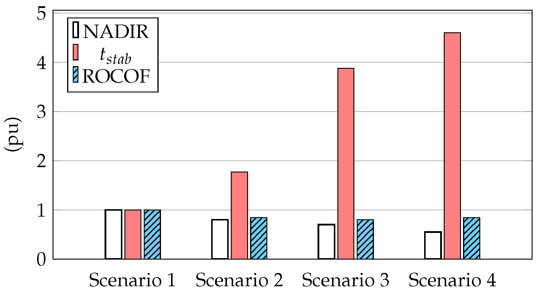
Figure 19 and
Figure 20 compare Nadir, stabilization time and Nadir for
. The increasing of the stabilization time in [
23] is due to the fact that when the wind power plant changes from recovery to normal operation mode, a third frequency shift occurs. Despite it is not so noticeable compared to the second frequency excursion, see
Figure 15a,
Figure 16a and
Figure 17a, it can achieve up to 70 mHz for scenario 4.
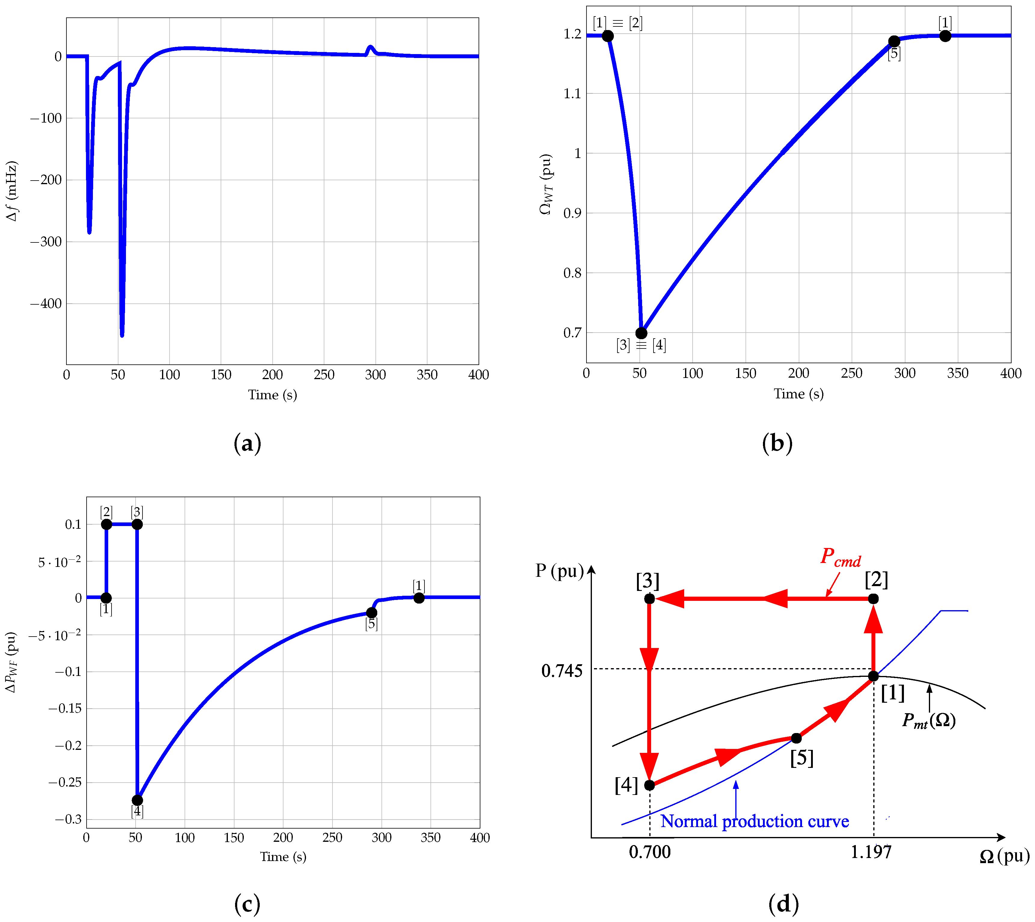
In
Figure 21 the wind power plant response of scenario 2 and
with the frequency controller of [
23] is depicted. Between points [1]–[2], the VSWT is working in the normal operation mode, providing its maximum power
pu. Because of that, the variation of active power provided is 0 (see definition of
in
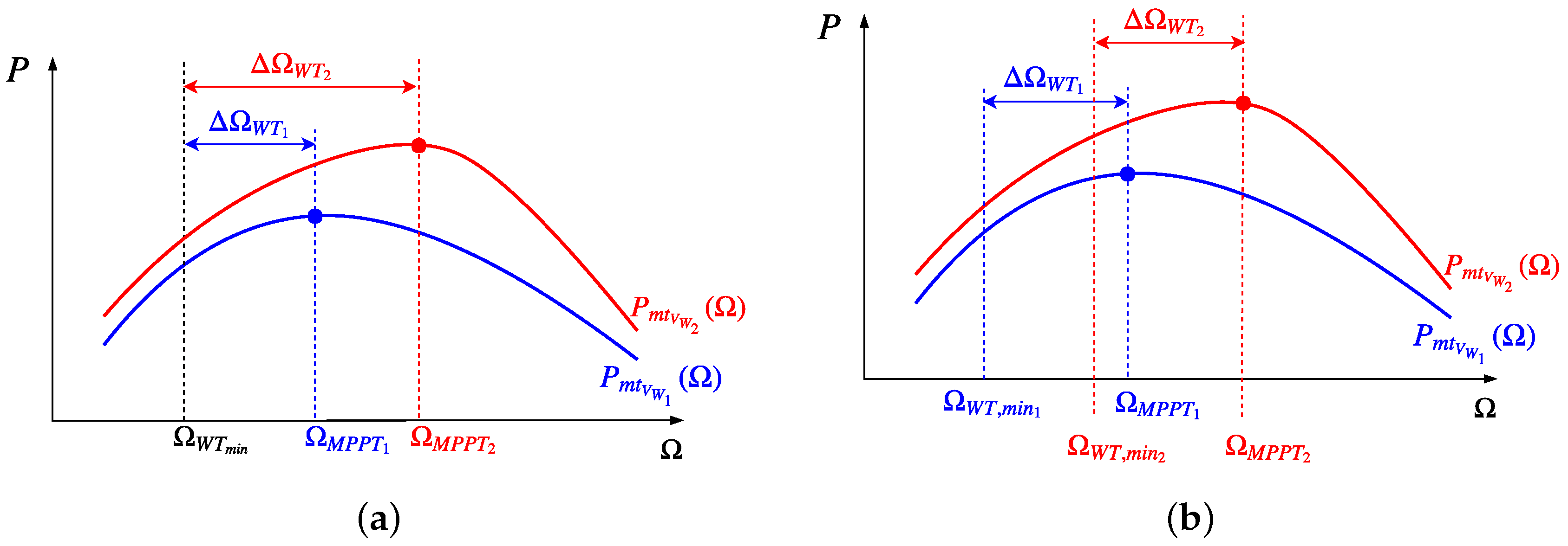
Section 2). The rotational speed of the machine is
pu. At time
s, the power imbalance occurs, activating the overproduction mode (points [2]–[3]). Hence, the variation of active power provided by the wind power plant is constant and equal to
pu. This value corresponds to the additional active power provided by the VSWTs in this operation mode,
, which is taken from the stored kinetic energy of the machine. As a consequence, the rotational speed of the VSWT decreases from
to the minimum value
pu, corresponding to a 42% of decrease in 30 s. When
reaches its minimum value, the frequency controller changes to recovery operation mode (points [4]–[5])). The sudden drop of the variation of active power generated (points [3]–[4]) causes a second frequency departure, being this deeper than that due to the power imbalance. This power variation is
pu. Apart from that, it is important to notice that it takes around 250 s to restore the rotational speed to the initial value
.
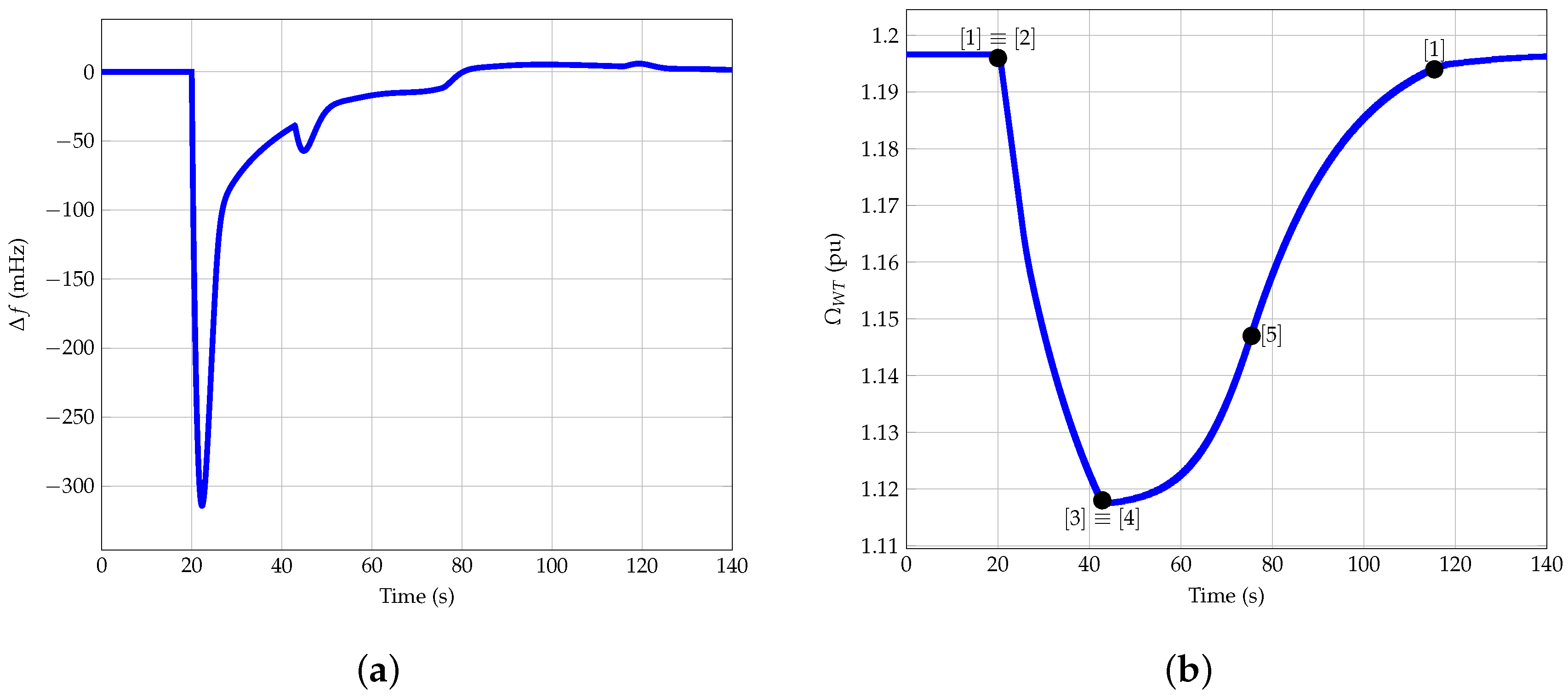
Regarding to
Figure 22, the wind power plant response of scenario 2 and
with the proposed controller considering
is shown. In this case, the rotational speed decreases from
to
pu in 20 s (points [2]–[3]). Despite it takes less time than in
Figure 21, the reduction of rotational speed is also lower, only 0.07%. Furthermore, the second frequency departure caused by the drop from overproduction to recovery (points [3]–[4]:
pu) is negligible in comparison to the one indicated in
Figure 21. The wind power plant needs only 80 s to restore the rotational speed to the initial value (points [4]–[5]). The equation of the parabola in this case is:
.

 ,
, 


