Quantitative Resilience Assessment under a Tri-Stage Framework for Power Systems

The State Key Laboratory of Electrical Insulation and Power Equipment, the Shaanxi Key Laboratory of Smart Grid, Xi’an Jiaotong University, Xi’an 710049, China
*
Author to whom correspondence should be addressed.
Energies 2018, 11(6), 1427; https://doi.org/10.3390/en11061427
Submission received: 26 April 2018
/
Revised: 25 May 2018
/
Accepted: 28 May 2018
/
Published: 3 June 2018
(This article belongs to the Section F: Electrical Engineering)
Abstract
:The frequent occurrence of natural disasters and malicious attacks has exerted unprecedented disturbances on power systems, accounting for the extensive attention paid to power system resilience. Combined with the evolving nature of general disasters, this paper proposes resilience assessment approaches for power systems under a tri-stage framework. The pre-disaster toughness is proposed to quantify the robustness of power systems against potential disasters, where the thinking of area division and partitioned multi-objective risk method (PMRM) is introduced. In the case of information deficiency caused by disasters, the during-disaster resistance to disturbance is calculated to reflect the real-time system running state by state estimation (SE). The post-disaster restoration ability consists of response ability, restoration efficiency and restoration economy, which is evaluated by Sequential Monte-Carlo Simulation to simulate the system restoration process. Further, a synthetic metric system is presented to quantify the resilience performance of power systems from the above three aspects. The proposed approaches and framework are validated on the IEEE RTS 79 system, and helpful conclusions are drawn from extensive case studies.
1. Introduction
Maintaining a high level of power supply reliability is one of the main requirements for power systems. Due to the development of smart grid technology, the use of new electrical materials and the interconnection of the regional power systems, the grid structure of power system has been strengthened substantially, greatly improving the reliability level under normal conditions. However, the increasing frequency of natural disasters and human attacks has led to a large number of blackouts and outages [1,2]. Thus, power system resilience has dominated the research of researchers and scholars in recent years.
Resilient power system could anticipate possible disasters, adopt effective measures to decrease system components and load losses before and during disasters, and restore power supply quickly [3,4,5]. Additionally, valuable experience and lessons can be absorbed from disasters suffered, to prevent or mitigate the impact of similar events in future. Panteli [6,7] discussed the difference between power system resilience and reliability. Reliability research [8,9] concentrates more on small-scale and random faults of power system components caused by internal factors. In contrast, under extreme disaster conditions, the occurrence possibility of wide-range components permanent failures will increase sharply; the common control and restoration measures are difficult to implement, greatly prolonging the duration of outages. Therefore, the study on power system resilience will provide technical support to improve the power supply reliability under all kinds of circumstances.
Power system resilience assessment can measure the capability of a system to maintain stable operation status and to provide sufficient power supply against disasters. The current methods of resilience assessment are mainly divided into three categories [10]: the simulation-based method [11,12,13], the analytic method [14], and the statistical analysis [15,16]. Panteli [17] developed the fragile model of the transmission system and presents a comprehensive assessment methodology for multi-temporal and multi-regional resilience. Wang [18] provided a quantitative analysis of the temperature and water availability effects on resilience of the power system. Four indices were introduced by Liu [19] to measure the grid resilience from different perspectives including fragility, survivability and restoration. The resilience trapezoid is discussed by Panteli [20], based on which the authors put forward a resilience metric system called “ΦΛEΠ”.
Considering the nature of disastrous events, it is reasonable to divide their effect on the power system into different stages: before, during and after the disturbance. That is because the main issues to be emphasized and the operating characteristics are quite different for these stages. The prevention, resistance and post-disaster restoration work against disasters is a long-term and multi-stage process, so it is of much difficulty to recognize and study the power system resilience as a single entity, which will expand the scale and increase the complexity of the research. Combined with the resilience curve, Panteli [6] firstly divides the stages of power system resilience, and gives the features that a resilient power system must possess at each stage. As an important part of resilience research, resilience should also be evaluated by stage to reduce the difficulty, regarding the evolutions of system states and disasters. Espinoza [21] proposed the points of multi-stage resilience assessment for the first time, and put forward an assessment framework consisting of four phases: threat characterization, vulnerability assessment of the system’s components, system’s reaction and system’s restoration. Panteli [20] innovatively proposed the concept of the multi-phase resilience trapezoid, and quantified the resilience of power systems based on the stages of disturbance process, post-disturbance degraded state and restorative state.
Existing resilience assessments, which are usually conducted before disasters, tend to regard the response, adaption and restoration process of power systems as a whole. However, these approaches cannot totally demonstrate the advantages of multi-stage resilience assessment, and the key problems of each stage cannot be revealed thoroughly. To consider the multi-stage characteristics of power system resilience, we divide the resilience assessment into three components: pre-disaster system toughness, during-disaster system resistance and post-disaster system restoration ability. We will define them in detail in Section 2. Furthermore, based on the three stages, assessment algorithms are synthetically proposed. Moreover, the existing metric systems are inadequate and over-simplified to reflect the ability of the power system to withstand destruction of disasters at all stages. A more complete assessment metric system is presented to assess resilience in this paper.
The remainder of this paper is structured as follows: Section 2 describes the outline and the necessity of the proposed three-stage power system resilience framework. The resilience assessment methodologies as well as corresponding resilience metrics of pre-disaster, during-disaster and post-disaster stages are discussed respectively. Numerical studies are provided in Section 3 to exhibit the effectiveness and application values of the proposed framework. Finally, the conclusions are drawn in Section 4.
2. Resilience Assessment under a Tri-Stage Framework
2.1. The Outline of the Tri-Stage Framework
In the face of disasters’ disturbance, resilient power grids should be robust, to decrease loss of component due to damage and load shedding. They should be able to restore curtailed loads efficiently by operational measures and repair dispatch.
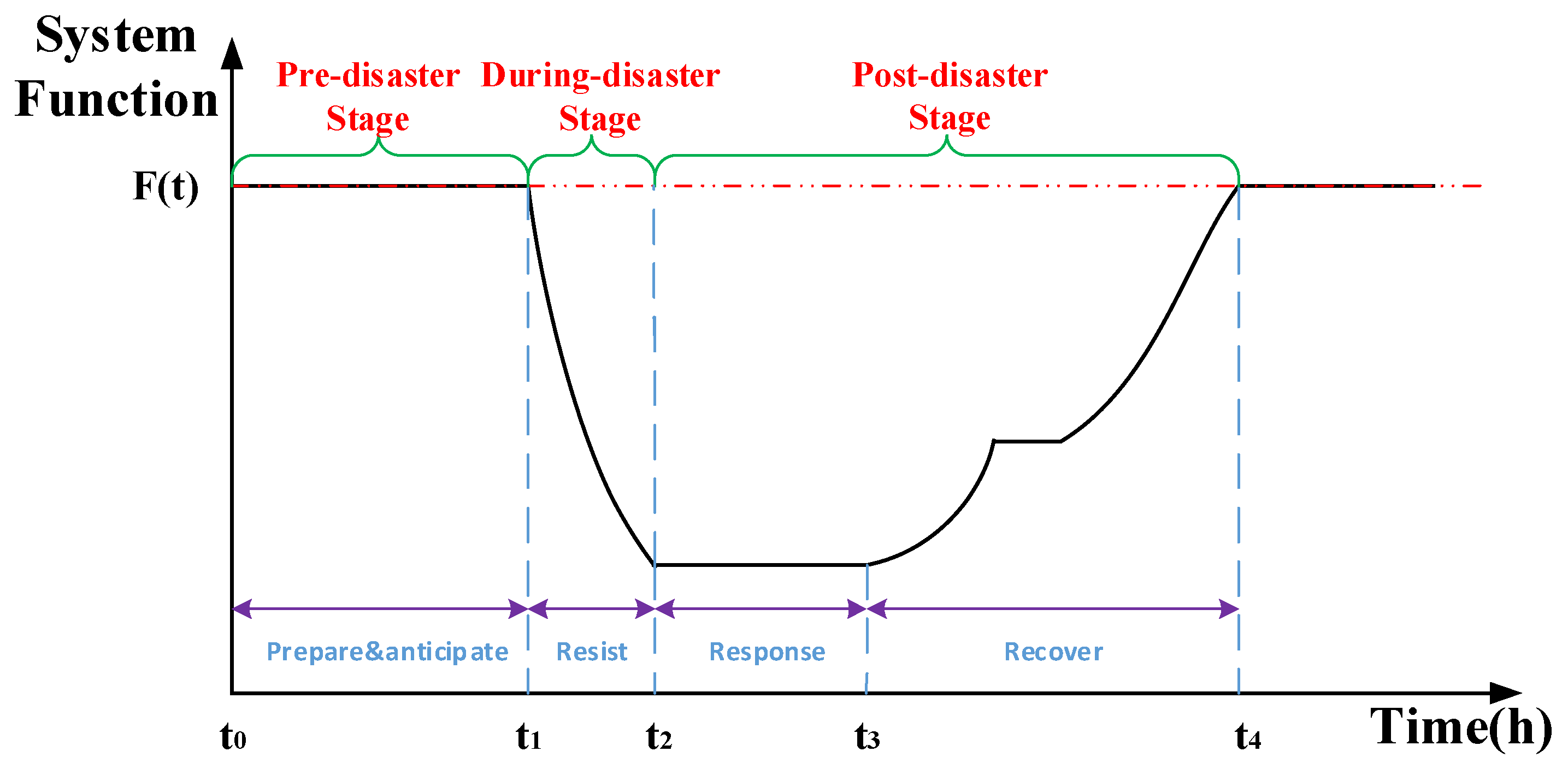
Further, in our view, a resilient power system should possess the following characteristics, which are the inspirations of the research. Before disasters, with high-definition meteorological forecast system, in most cases of natural disasters, the power system can analyze the possible landing area of the event in advance, predict the characteristic of forthcoming disasters, and take preventative measures. During disasters, instead of passively waiting for the disaster to end, efficient operation and control measures can be adopted to alleviate the destructiveness to equipment and power supply. After disasters, the restoration schemes can be formulated rapidly to realize fast component repair and load restoration. All three aspects are indispensable to “resilience”, and they are reflected in Figure 1.
Therefore, the assessment of power system resilience should also come to be implemented in line with the three stages: pre-disaster, during-disaster and post-disaster:
Pre-disaster Stage: we define the concept of “toughness” to represent the pre-disaster resilience and reflect the expected robustness of power systems against disasters. The toughness assessment methods under different types of disasters are established. Given the type, the intensity, the duration and the range of possible disasters, the particular system operation situation will be calculated through simulating the damage-repair process of components. The toughness metrics are formed from three perspectives: the expected damage degree of system, the risk of system splitting, along with the generation and transmission margins. Besides, we are the first to propose the concept of “area division” and “partitioned multi-objective risk method” in toughness assessment.
During-disaster Stage: relying on the advanced Cyber Physical System, the component state information and power system running condition can be obtained rapidly. Based on this prerequisite, the real-time system resistance metrics are proposed to quantify the current damage and load loss degree of system. Moreover, when disaster happens, sometimes the cyber system will be impacted as well. In this case, state estimation is adopted to measure the actual operation level, which provides decision-making basis for during-disaster emergency control.
Post-disaster Stage: Under the premise of obtaining system damage information and restoration scheme, Sequential Monte Carlo Simulation (SMCS) is used to depict the dynamic restoration process of power systems. The quick response, restoration efficiency and restoration economy are concentrated to evaluate the system post-disaster restoration ability, helping to compare different restoration schemes.
For the convenience of the reader, following sections are organized based on the tri-stage framework mentioned above. Each section will firstly present evaluation metrics to highlight the keys concerns of each stage, and then discuss resilience assessment algorithm and approach.
2.2. Pre-Disaster Assessment Stage
The resilience pre-disaster assessment stage consists of a “toughness” assessment, that is, the expected capability of power systems to keep stable operation and provide continued power supply for users against disasters. The core of toughness assessment is to analyze the possible damage and losses due to specific disasters in advance, which is the basis for disaster hazard prediction and loss mitigation.
Toughness, as an inherent performance of resilient power systems, is primarily determined by grid structure, equipment strength and smart operational measures. However, the duration time, characteristics of occurrence and damage mechanism to components of different high impact/low probability (HILP) events vary greatly, so even the toughness of the same power system will act differently under different circumstances. Concrete toughness analysis is needed under specific disasters.
2.2.1. The Metrics of Toughness
This paper proposes some metrics to reflect the toughness of power system from three aspects: the expected damage degree of system, the risk of system splitting, along with the generation and transmission margins.
● The expected damage degree of system
When the system is hit by disasters, the direct impact is the load loss due to the breakdown of components, which emphasizes the necessity of evaluating the expected load and component loss situation against disasters.
The loss of load probability (LOLP) and the expectation of demand not supplied (EDNS) are suitable for the assessment of toughness, and the definition of them can be found in [22].
Average load loss ratio in case of load curtailment (ALRIL), represents the average proportion of load loss to the whole current load demand, which is:
where Ns indicates the whole simulation times, and Llc,i represents the amount of load shedding in the ith simulation (the simulation method is presented in the next part). Ld,i is the load demand of system in the ith simulation.
The probability of components failed during disaster (PCFD) is:
Nc,i is the number of the failed components in the ith simulation, and Nc indicates the number of the whole components. The noteworthy thing is that PCFD should be calculated according to the types of vulnerable components separately.
● The risk of system splitting
When a large-scale disaster happens, the risk of system splitting or some nodes being isolated will increase, as components faults may create isolated parts in the system. The following two metrics are introduced to address these possibilities in the evaluation framework.
The possibility of system islanding (PSI) and isolated note (PIN), as in Equations (3) and (4) respectively:
Nsi is the number of simulations where system islanding occurs and Nin is the number of simulations where isolated node exists among the whole simulation times Ns.
● The generation and transmission margins
Power systems can be divided into several areas with close electrical connections, according to the impacted areas under disasters and the electrical characteristics of the system. Usually, the neighboring areas are linked by several transmission lines, which make up the transmission section. Currently, it is widely-used practice to divide the post-disaster system into several parts, and each part is restored in parallel. This parallel restoration adopts a simpler restoration strategy at each area while accelerating the restoration process, and can guarantee system stability.
Therefore, the generation margins of areas (GMA) and the transmission margin of transmission section (TMTS) between different areas are proposed, to reflect the expected maximum generation capacity within the area and the expected transmission capacity of the section against disasters:
- Gg,max The maximum real power output of unit g;
- Lb,real,u The real load amount on bus b under disasters;
- Lb,real,be The real load demand on bus b before disasters;
- Gnow The set of normal units within the area under disasters;
- Gall The set of normal units within the area before disasters;
- Ball The set of all buses within the area;
- Ck,max The power transmission upper limit of line k;
- Ck,u The power flowing on line k under disasters;
- Ck,be The power flowing on line k before disasters;
- lnow The set of normal lines among the transmission section under disasters;
- lall The set of normal lines among the transmission section before disasters.
If the value of generation margin is small or even negative, it indicates that there will be a serious shortage of power generation within the area, and this will lead to higher internal load shedding risk once the transmission lines are damaged. Conversely, large value of generation margin means the sufficient regional power generation, which will help to avoid load loss.
If the value of transmission margin is small, it indicates that the transmission capacity of the section will be restricted dramatically, so the power demand of different areas is mainly supplied by their internal generation. By contrast, the large transmission margin means that the transmission capacity of the section is not badly disrupted.
2.2.2. Toughness Analysis Based on PMRM
Under disaster conditions, the probability of high-loss and medium-loss damage situations increases greatly, so the average-risk-based assessment metrics cannot fully reflect the severity of serious damage. PMRM, which was first proposed by Acbeck and Haimes in 1984 [23], helps to show high and medium risks by analyzing the conditional probabilities and the conditional risk expected values (CREV). Hence, PMRM is also applicable to toughness analysis.
To illustrate the practical value of PMRM, it is used to analyze the toughness of power systems, by taking “EDNS” for example. The following two metrics are proposed according to the proportion of expected load loss (the value of EDNS) to the system load demand. We use the load loss ratios of 5% and 25% as the segmentation points. The load loss intervals of low loss, medium loss and high loss are designated as 0~5%, 5~25% and 25~100% separately.
Ri represents the expected load loss under low-loss, medium-loss and high-loss situations:
Pi represents the conditional risk probability under low-loss, medium-loss and high-loss situations:
SL, SM, and SH are the sets of low-loss, medium-loss and high-loss events. P(j) is the occurrence probability of the load shedding event j, and the corresponding amount of load curtailed is Loss(j). pL, pM, and pH are the occurrence probabilities of low-loss, medium-loss and high-loss events.
When the CREV or high-loss and medium-loss conditional probabilities exceed the warning boundaries set by decision makers, it is hard for power systems to resist a given disaster. Under this circumstance, it is urgent to take measures to reinforce and update the system, which effectively mitigate the serious harm and reduce the risk of cascading failures.
2.2.3. The Procedure of Toughness Assessment
Taking windstorms and lightning as examples, the toughness assessment procedure under different types of disasters is introduced. This paper refers to the idea of reliability evaluation and risk assessment, and divides the procedure of toughness assessment into several parts.
● The identification of disasters characteristics
To accurately analyze the toughness of power systems, we should make sure which type of disaster is to be considered. The probable affected region, and the duration and intensity of disasters should be identified at first. In this paper, windstorms and lighting are discussed to evaluate the resilience of the power system.
● The acquisition of the type and the failure/repair rates of vulnerable components
The types of vulnerable components vary greatly under different disasters. For example, cyber- attacks will impact communication and information storage devices (such as EMS and SCADA); earthquakes will presumably destroy substations; transmission towers and lines tend to collapse during high winds. By identifying the different disasters, we can determine the temporal and spatial damage mechanism on power system of disasters, identify the type of vulnerable components and then acquire their failure/repair rates.
It is widely accepted that the quadratic model is suitable to describe the pressure exerted on transmission lines by winds. The failure rates of transmission lines are formulated to be proportional to the square of the wind speed [24,25]:
when the wind speed is below ωcrit, λwind = λnorm.
The average repair time is regarded to be constant for wind speeds below ωcrit [24] and increases linearly for higher wind speeds. The repair time for transmission lines under windstorms can be defined as:
where ω(t) is the wind speed at time t; α is a scaling parameter; ωcrit is the critical wind speed over which λ is increased; λnorm is the constant failure rate under normal condition; rtnorm is the reference repair time under normal condition and k is the repair time growth rate with ω(t).
In order to compare the effects of different disasters on the toughness of power systems, the lightning is analyzed as well. The line failure rate under lighting strike conditions is obtained from [26], as shown in Equation (11), where a linear relationship is used, considering the ground flash density:
Based on what is suggested by Cadini [26], the repair rate model of transmission lines is built as:
where rrnorm is the sonstant repair rate during normal conditions; μ, β are scaling parameters; and Ng is the number of ground-flashes per unit of time and area (occ/h*km2).
● State sampling of components
Power systems are traditionally designed to sustain single outage contingency (“N-1” security criterion). However, multiple and large-scale component faults may happen during HILP events.
Generally, to mitigate the outage, faulty component repair work should be carried out, especially for long-duration disasters, such as windstorms. Therefore, the procedure of failure-repair-failure needs to be taken into account. SMCS is suitable to sample the states of vulnerable components.
As for short-duration event, such as earthquake or lightning, the repair work is usually not assigned until the end of disasters. Sometimes disasters (like floods) may be so severe that the repair work cannot be implemented for the safety of repair crews. In this case, Nonsequential Monte Carlo Simulation is adopted to sample the state of components, allowing the failure possibility of vulnerable components to be determined
Due to the lack of related mathematical models, we combine Equations (11) and (12) to establish the failure possibility model of transmission lines from a statistical point:
● State analysis of power system
After obtaining the state of each component, the power system state should be analyzed. To reduce the losses of outage, this paper takes the minimum amount of load shedding as the objective and uses DC OPF to solve the problem if necessary. Then the metrics proposed in Section 2.2.1 are calculated.
2.3. During-Disaster Assessment Stage
With the continuous progress of smart grid and the Cyber Physical System, power systems will be gradually coupled with the information system as a whole. Consequently, the information of failure detection and load losses during disaster will be collected and transferred rapidly. Accordingly, resilience in during-disaster stage refers to the real-time resistance to disasters of power systems and reveals the actual running state of the system.
2.3.1. The Metrics of During-Disaster Resistance
Current load loss percent (CLLP) presents the load loss level of power systems under disaster destruction, which is:
where Lnl,b represents the load demand of bus b under normal conditions; Ldl,b is the actual load amount of bus b during disasters and Nb is the number of buses of the power system.
The available transmission capacity of the section (ATCS) indicates the damage situation of the transmission section:
where Ck,d is the power flowing on line k during disasters and lduring is the set of normal lines among the transmission section during disasters.
The active power deficiency of the area (APDA) represents the real power vacancy of the area where the generation is insufficient. The load within the area has to be supplied from external areas:
where Gg,d is the real power output of unit g during disasters and Gduring is the set of normal units within the during-disaster area.
2.3.2. The Method and Procedure of During-Disaster Resistance Assessment
The advancement of information technology increases the degree of cyber-physical coupling of the power system. However, a serious natural disaster may cause damage to measurement devices and the malfunction of monitor systems, making it difficult to evaluate the damage situation and operation state of the power system. Under this circumstance, SE should be adopted to solve this problem.
SE can “convert the measurement redundancy and other available information into an accurate and integrated estimate of the state of the power system” ([27], page 1), especially for the areas where the data is missing or difficult to measure. This technique provides an emergency solution to evaluate the running condition of power systems and makes up for the loss of measurement devices, as well as assists the reliable dispatching of the state of the power grid when a large-scale disaster comes. The vector of the voltage magnitudes and angles of all buses can represent the state of power systems [28]. For a power system containing Nb buses, its 2Nb − 1 dimensional state vector is shown as follows:
Vb and δb are the voltage amplitude and angle of bus b respectively.
The state vector will be updated through the iteration of SE, which minimizes the residuals between the measurements and the corresponding estimate values. Then the actual lost measurements can be estimated.
During disasters, it is assumed that the system state data gathered from the remaining real-time measurement device is included in the m dimensional measured vector. For example, the measured vector of bus b is chosen as:
where Pb and Qb are the active and reactive load on bus b. Pk,b and Q k,b are the active and reactive power flowing on line k, which are injected from or to bus b. Nn,b is the number of measurements of bus b. Due to the uncertainty of the damage, the remaining measurements of each bus may differ in number and types.
In line with the elements of the measurements vector z, the actual system state ztrue can be calculated from the measurement functions h(x), which can be expressed by the nonlinear equations of the state vector x:
Here the term hb (x) represents the measurement functions of bus b:
Due to the minimal computational requirements, the Weighted Least Square (WLS) method is the most common algorithm for SE to reduce the estimated residuals. The objective of the WLS method is given in Equation (21) and the SE results are obtained by its iterative solution:
where the measurement error covariance matrix R indicates the weights of confidence for each measurement.
Based on the WLS algorithm mentioned above, the SE procedure of the disaster-hit areas with information loss is listed as follows:
- Initialize the variables.Read the remaining measured vector z and set the origin values of the state vector x(0).
- Calculate the measurement Jacobian matrix H(x(k)).The equations of H(x(k)) is shown as below:
- Judge the observability of system through the gain matrix G(x(k)), which can be formulated from H(x(k)) and R [28]:where the k indicates the kth iteration.
Add the historical data to the measurements vector z as pseudo measurements if the measurement redundancy is too low or G(x(k)) is even singular.
- Calculate the modification vector as:Then update the state vector by:
- Keep iterations until the convergent criterion is satisfied. Then the results will be the current state vector .
- Calculate the actual system state ztrue and during-disaster resistance metrics.
By fitting the remaining measurements from normal areas to the measurement functions, the missing measurements can be estimated entirely and precisely.
2.4. Post-Disaster Assessment Stage
After disasters, the most essential and critical task is to apply the optimal system restoration scheme, with the minimal cost of money and time. This section describes the assessment metrics of post-disaster stage and the assessment procedure from the perspective of response ability, restoration efficiency and restoration economy.
2.4.1. The Loss Assessment after Disasters
The loss assessment after disasters is similar to the method in Section 2.3.2. Correct assessment of losses can help to calculate the disaster damage to power grids, and guide the formulation of response and restoration plans.
Post-disaster load loss percent (PLLP), which resembles CLLP, is calculated by:
where Lpl,b is the actual load amount of bus b in the post-disaster state without restoration.
Besides PLLP, AFS is defined to represent the average falling speed of the system performance, i.e., the ratio of load loss divided by the duration of disaster (just for long-term disasters):
where tld is the duration of the disaster.
2.4.2. The Metrics of Restoration Ability
No effective assessment method for post-disaster restoration ability or evaluation metric system is studied thoroughly. In this paper, the restoration ability is defined to be comprised of response ability, restoration efficiency and restoration economy.
● Power system response ability
The response ability measures the ability of power systems to take quick action after disasters. A system with fast responsiveness will restore electricity for users as soon as possible, improving the reliability of power supply dramatically:
(1) The length of time from the end of disaster (ted) to the start of load restoration (tsl), LEDSR, shows the period when the system remains in the post-disaster worst state.
(2) The ratio of load restored in one hour after tsl (RLRO):
where L1h,b is the restored load amount of bus b in one hour after tsl.
(3) The length of time from ted to when the load of the system recovers to the specified proportion, could be represented by tsp. The proportion of load could be designed according to the power grid operation state considering social benefits.
The above three metrics can reflect the response ability of power system after disasters.
● Power system restoration efficiency
The restoration efficiency assessment outlines the effectiveness and practical value of the restoration scheme. The average restoration speed of system load (ARSS), the restoration efficiency of system load (RES) and the restoration efficiency of the important load (REI) are the three metrics to evaluate the restoration efficiency:
where tre is the time when the system load restoration process ends. The load on bus i is split into ni parts according to the importance. The load loss at tsl after disasters is pij and pij(t) is the actual load loss j on bus i at time t during power restoration. In essence, ARSS is the ratio of power losses avoided to power losses without restoration:
The weight factor of load j on bus i is wij:
where pid is the important load loss on tsl after disasters on bus i, and pij(t) is the real important load loss j on bus i at time t during power restoration.
Restoring the important load (e.g., hospitals, government and rescue dispatching center) at first can significantly lower power losses and avoid adverse social impacts. Therefore, this emphasizes the evaluation of the ability to restore the important load.
● Power system restoration economics
In order to realize the fast restoration of the outage, the economic cost will not be the most important issue for decision makers. However, a good restoration scheme is capable of restoring the system quickly and efficiently with the minimum economic cost. Hence, it is necessary to assess the economy of the restoration schemes (RSE). The load economic losses, and the repair costs, such as material, labor, transportation, and generator fuel, should be considered:
The economic loss of load j in unit time on bus i is cij, and Crep is the economic cost of the repair work.
2.4.3. The Procedure of Restoration Ability Assessment
Because of the scarcity of extreme disasters and the construction of regional interconnected power systems, the ability of power system to resist disturbance has been greatly improved, leading to the lower probability of large-scale blackouts. In addition, reasonable protection and automatic devices, along with advanced alarm processing and fault diagnosis technology, can restrict the electrical faults in the local area. Therefore, it is more meaningful and practical to study the restoration of local power system after disasters. Correspondingly, a novel power system post-disaster restoration ability assessment process is discussed in this part.
Some assumptions are made to simplify the calculation and analysis:
- (1)
- The system repair scheme ensures that there will not be a shortage of repair personnel or materials in the repair process of each fault point.
- (2)
- The post-disaster Mean Time to Restoration (MTTR) of fault components is the same as that under normal condition.
- (3)
- The route time of the repair team is determined by the distance, vehicle speed, the traffic flow and the traffic capacity of road.
- (4)
- Each fault point is repaired by only one team. Once a fault is repaired, the repair crew will go to the next one immediately.
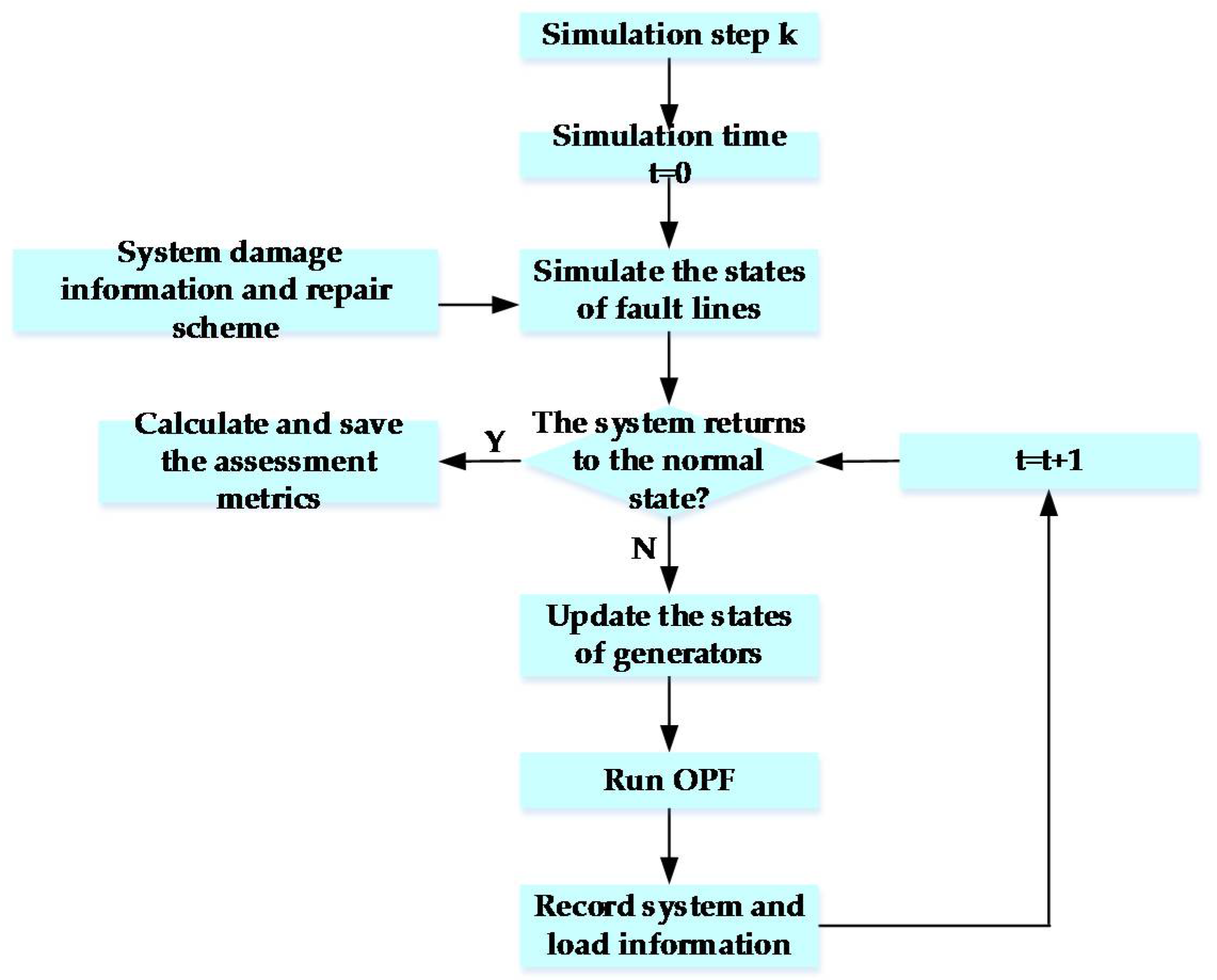
In this paper, the restoration ability assessment takes the repair of fault lines, the re-operation of the generating units out of service, the ramp speed constraints of generators and the output of distributed generation (DG) into account. Figure 2 shows the simulation procedure.
● The acquisition of damage information and restoration schemes
The location of fault points, the types of fault components, the power network topology and the geographic information should be obtained. The assignment and route of each repair team, and the available DG at load nodes should be clarified explicitly.
● State sampling of failure components according to the sequence of repair
Given the restoration scheme, the state sampling is conducted to simulate the evolutions of fault component states, while SMCS is used for this simulation. The time it takes for the line to return to the normal state is mainly composed of three parts: the waiting time, the route time of repair teams and the repair time. The BPR function is used to model the route time [29]:
where t0 is the free travel time, V is the traffic flow, and C is the capacity of road traffic. m is the regression coefficient. The repair time of a single fault point is subject to exponential distribution:
where tmttr is the mean time to repair, and u is a random number distributed uniformly between 0–1.
● State analysis of power system
The calculation method in this part is the same as that in Section 2.2.3. It is important to note that, to improve the efficiency of restoration, the important load at each node has to be restored in priority.
● The calculation of power system restoration metrics
The metrics are calculated to reflect the restoration ability of the power system. The restoration curves of fault equipment and load curtailed should be depicted as well. The assessment of power system post-disaster restoration ability reflects the effectiveness and economic benefits of restoration strategies, and helps to assess and compare the pros and cons of different restoration scenarios.
3. Case Study
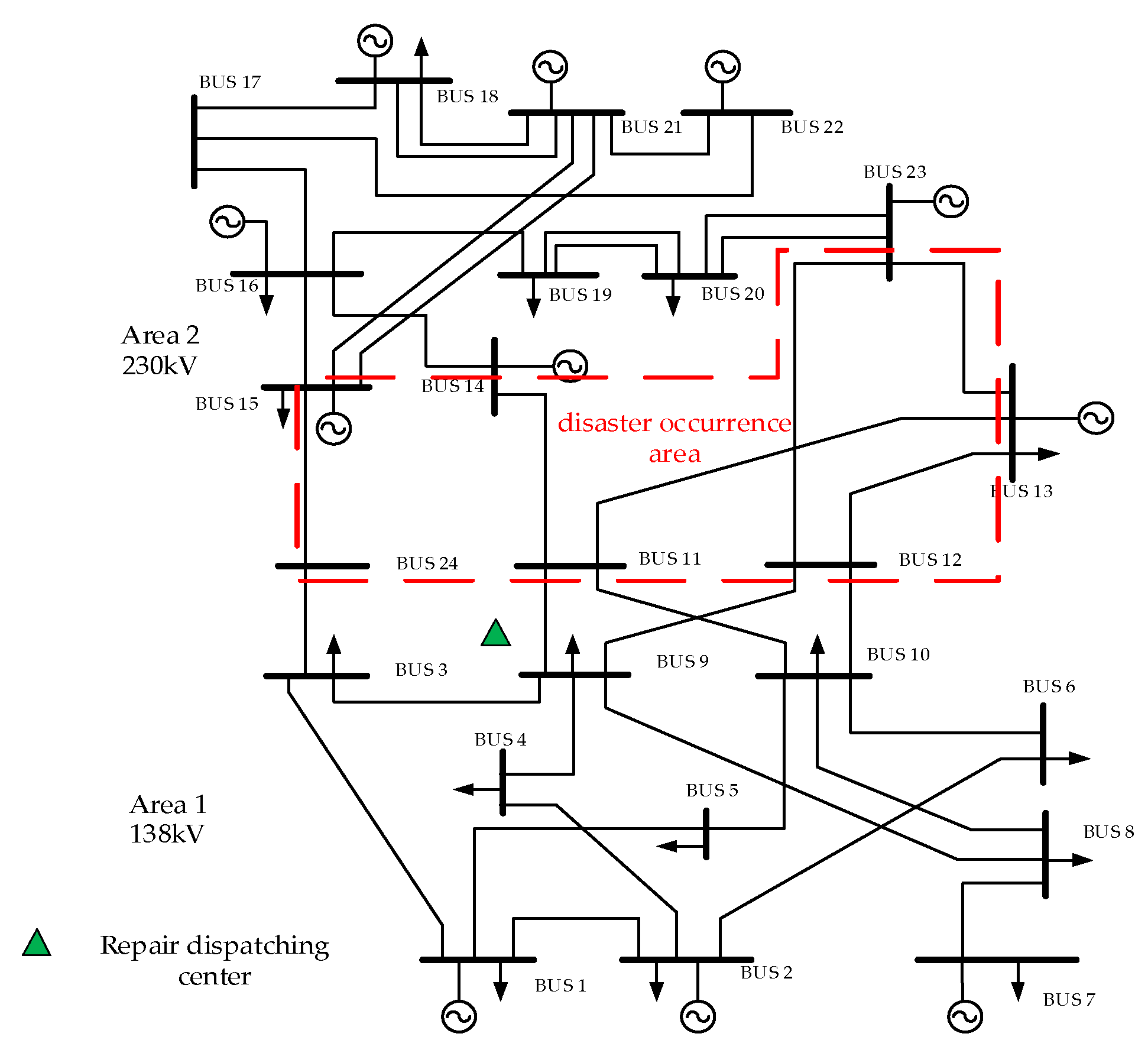
The tri-stage resilience assessment framework is illustrated by assessing the impacts of windstorms and lightings on the IEEE RTS 79 system [22]. To highlight the severity of disasters, the system load is fixed to 2850 MW, the annual peak load of the system, during the whole assessment process. According to the voltage levels, the system is divided into two areas: Area 1 (bus 1~12, 24) and Area 2 (bus 13~23). It is assumed that line 18 (11–13, 53 km), 19 (11–14, 47 km), 20 (12–13, 53 km), 21 (12–23, 108 km), and 27 (15–24, 58 km) are hit by disasters, as shown in Figure 3.
3.1. Pre-Disaster Resilience Assessment
3.1.1. The Resilience of Power System under Different Types of Disasters
The power system is assumed to locate in a tropical coastal area. To resist the damage from strong winds, the design and construction of transmission systems are resilience-oriented. That is to say, when facing the common storms, transmission lines can operate normally, and their failure probabilities are lower than those of ordinary lines.
It is assumed that the power system is hit by windstorms and lighting separately. Since the system is capable to resist the disturbance of ordinary high winds, ωcrit is set to be 25 m/s. A simulation time of 16 h and an hourly simulation step are adopted for toughness assessment under windstorms. ω(t) is assumed to be 38 m/s (the wind speed of a typhoon). By contrast, the toughness of the system against lightning (Ng = 0.1 occ/h·km2) is also evaluated. Values of scaling parameters in Equations (9)–(12) are assigned in Table 1 according to [25,26].
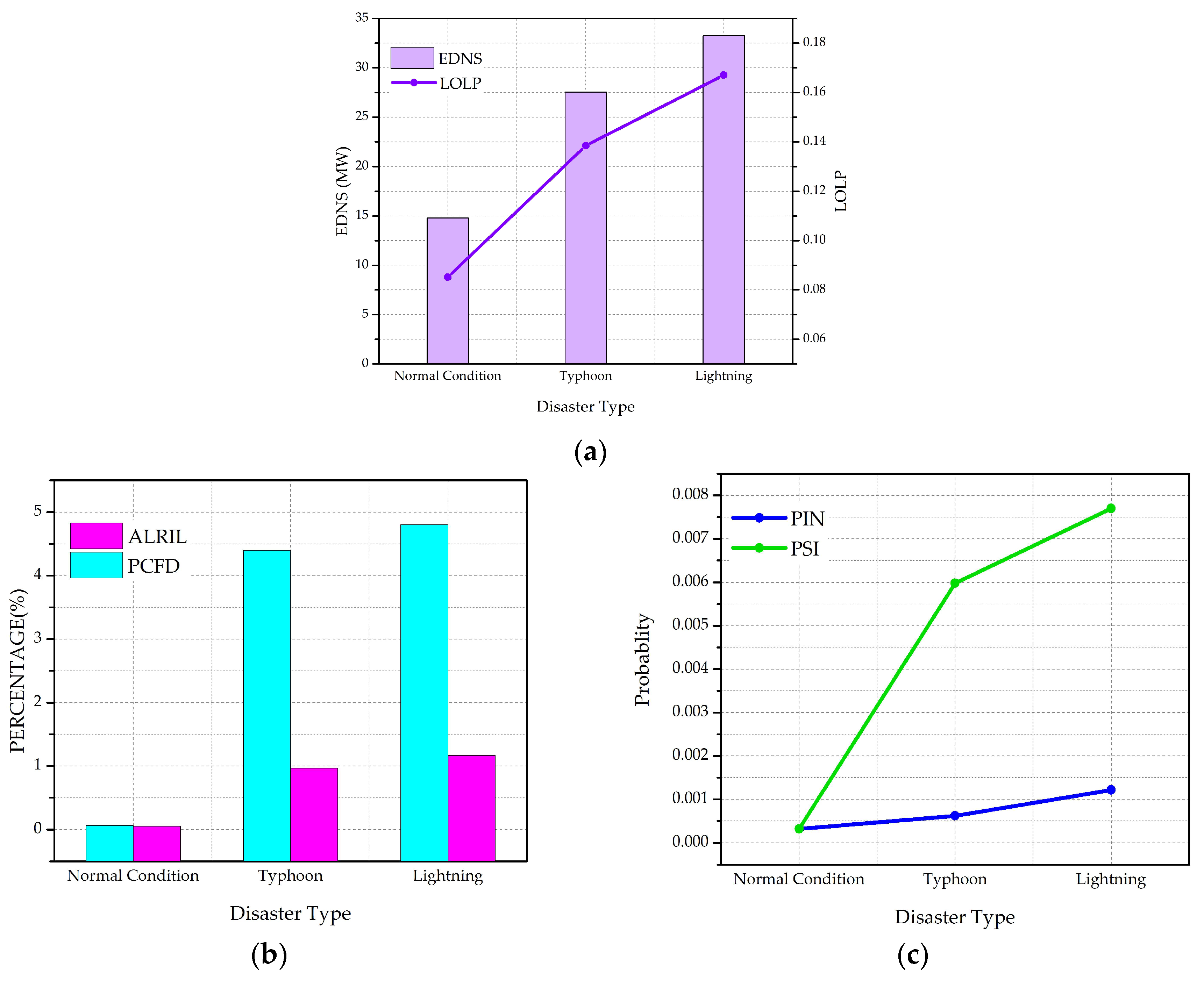
The assessment results are shown in Figure 4. From the normal condition to typhoon and lightning, it can be seen that the probability and the expected value of load shedding continue to rise, and more transmission lines are likely to break down, with the emerging possibility of isolated node and system splitting.
When facing disasters, the power transmission capacity of the section is tremendously limited, and consequently the power demand of each area is mainly supplied by the output of internal generators. Restricted by the range of affected region, disasters affect the transmission capacity of the section, not wrecking the generators. As a result, the generation margin of each area does not change much under different types of disaster. However, Table 2 indicates that the generation margin of Area 1 is of serious shortage, so the possibility of load shedding is extremely high in Area 1. By contrast, seldom does the load shedding occur in Area 2. Decision makers could consider allocating more generator capacity in Area 1 to raise the power generation reserve, strengthen existing transmissions lines or build more lines to improve the transmission capacity of the section.
Besides, the toughness of the power system against typhoon is stronger than that against lightning, even though the fury and threat of typhoons are much greater. That is because the power system has the capability to resist the disturbance of windstorms. For this reason, the assessment of resilience needs to be combined with the concrete types of disaster, not simply to say whether power system resilience is strong or weak.
3.1.2. The Resilience of Power System under Different Hazardous Intensity
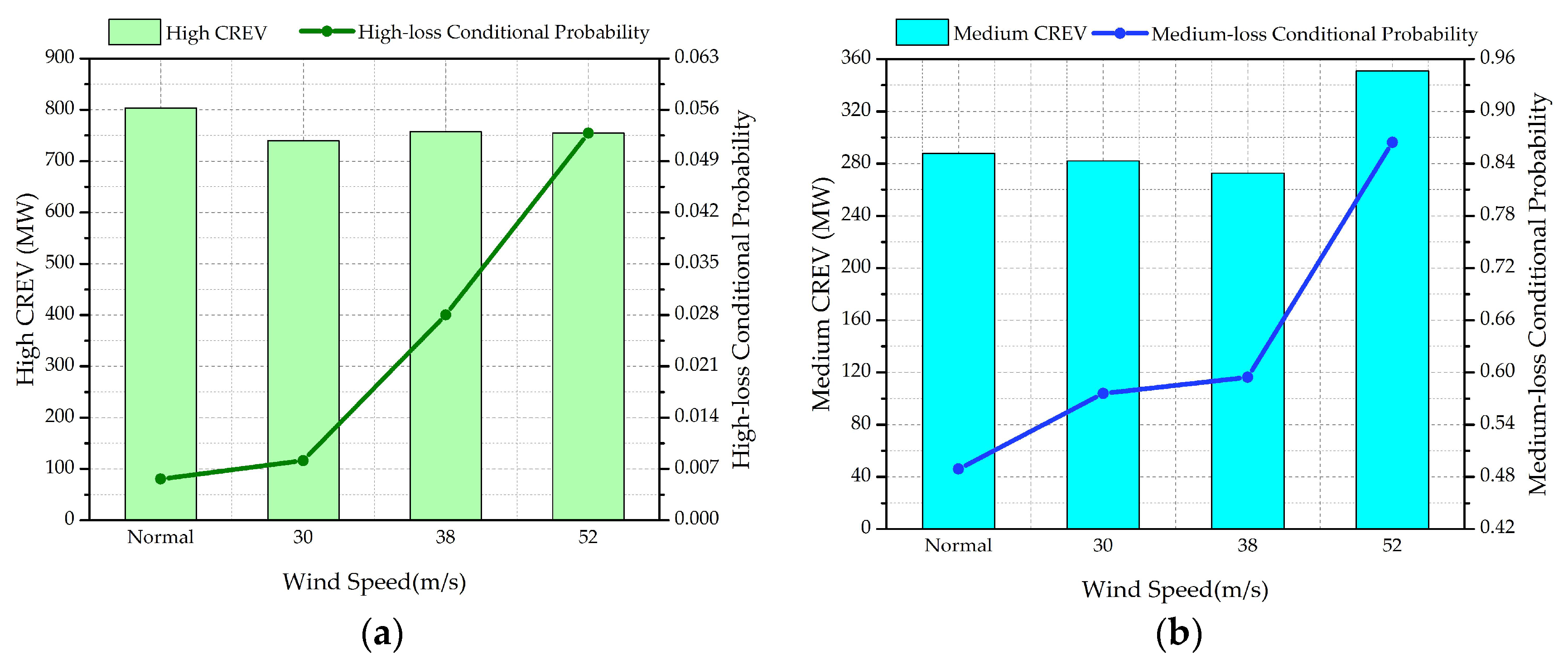
In this part, we evaluate the power system toughness under windstorms with four wind speeds, including normal environment, strong tropical storm (30 m/s), typhoon (38 m/s) and super typhoon (52 m/s), and analyze the expected risks the power system may face through PMRM.
From Table 3 and Figure 5, it can be observed that, on the one hand, with the rise of disaster intensity, the values of EDNS and LOLP increase sharply. The transmission capacity of the section drops gradually, and the risk of system splitting rises simultaneously. On the other hand, it can be seen that the more violent storm will result in higher medium-loss and high-loss conditional probability. When load shedding happens, the cases of medium and high loss are more likely to occur, causing more serious consequences. Besides, if the disaster strikes the power system in a wider range, the differences of CREV under windstorm conditions with different wind speed will be presented more obviously.
3.2. During-Disaster Resilience Assessment
3.2.1. Method Validation
In this part, the effectiveness of SE in Section 2.3.2 is validated. First, based on AC power flow, all the situations, where transmission lines normally work with different-order measurement loss, are estimated. And the errors between the actual and estimated values of power flowing on lines are tabulated in Table 4, showing the satisfying effect of SE.
The “order” means the degree of measurement loss due to the breakdown of the measurement devices. For example, the mode that the sensors of line 12–13 and 11–14 are destroyed is called the two-order measurement loss, and consequently it makes the two affected lines unmeasurable. Limited by the area hit by disasters, the higher orders of measurement loss are neglected for their bad convergence. It is necessary to note that all the remaining measurements are set to have the same confidence since we mainly focus on the feasibility of the method.
From Table 4, it can be observed that the difficulty of SE increases along with the rise of orders. The larger-scale loss of the measurement devices will sharply reduce the accuracy of the results estimated.
To explain this further, another two cases are studied. In both cases, all the lines’ measurements mentioned are lost, which means that their states cannot be collected directly. In the first case, line 12-13 fails to work, but line 11–14 continues to work; while in the second case, only the line 12–23 still operates normally. The calculation results of the two cases in Table 5 clearly show that the active power flow of line 11–14 and line 12–23 can be estimated accurately although the corresponding measurements are lacking, which verifies the effectiveness and accuracy of during-disaster system SE.
What’ more, it should be noted that if the unmeasurable lines are out of work, the estimated values will be 0. When the estimated values are non-zero, it indicates that transmission lines are still working, and then Dispatchers have to judge the running state of these lines. Emergency control measures should be executed once there is overload on lines, which is discussed in Section 3.2.2.
3.2.2. Method Application
It is assumed that there is a four-order measurement loss, including line 11–13, 11–14, 12–13, and 12–23. In this case, line 11–13, 11–14, 12–13 break down, and only the line 12–23 still works normally. The estimation result of the power flowing on line 12–23 is presented in Table 6.
It can be observed that the capacity limit of line 12–23 is exceeded. Due to the failure of line 11–13, 11–14 and 12–13, line 12–23 becomes one of the only two lines linking Area 1 and Area 2. From the assessment result in 3.1.1, the generation margin in Area 1 is insufficient, and its internal load is massively supplied by the power transmitted from Area 2, especially the output of generators on bus 13, which accounts for the reason why the line 12–23 is overloaded.
After adjusting the outputs of generators on bus 1, 2, 7, and 13 (see Table 7), the power flow of the remainder lines among the transmission section returns to the normal range, which is also proved by SE results after adjustment. Apparently, SE provides reliable data and information reference for emergency control, making up for the lack of measurement devices during disasters.
Accordingly, the during-disaster resistance metrics of the system are shown in Table 8. Due to the adjustment under emergency condition, the load shedding is avoided, which explains why CLLP is 0. The little value of ATCS and the large value of RPVRA demonstrate the high load shedding risk in Area 1.
3.3. Post-Disaster Resilience Assessment
It is assumed that after the duration of 16 h, the windstorm ends up. Line 18, 19, 20, 21, and 27 are destroyed. The distribution of load shedding is shown in Table 9. The proportion of different kinds of loads on each bus is assigned as 10%, 20% and 70% according to their importance, and the corresponding weight factors are 1.2, 0.8, and 0.3.
The capacities and the beginning operation moment of DG (on important load) are listed in Table 10, while the ramp speeds of DGs are neglected.
The locations of fault points are listed in Table 11.
The second row refers to the distance between the two adjacent fault points, while the first element in each item is the distance between the nearest fault point on each line and repair dispatching center.
3.3.1. Losses Assessment Result
Disasters destroy the transmission section, and the system splits into two islands, which operate independently, resulting in about the 1/5 loss of the system’s load, as shown in Table 12. The nodes with load loss are totally located in Area 1, whereas there is no load loss in Area 2. From the above toughness assessment, the generation margin is insufficient in Area 1 but sufficient in Area 2, which is also proved by the post-disaster losses assessment.
3.3.2. Restoration Ability Assessment Result
Assuming that within 15 min after the end of the disaster, the post-disaster repair and restoration scheme is formulated, and repair teams immediately set out to the fault points. The speed of repair team is designated to be 60 km/s under normal circumstances. Since the road traffic flow is large after disasters, the value of V/C is set to evenly distribute between 0.8~1.2. The value of m is set to 4.0 [29]. The average repair time of each fault point is 11 h [22].
The economic loss of lost load is considered to be $10,000/MWh [30,31] for really important load, $6979/MWh for commonly important load, and $3816/MWh for ordinary load. There are five members in each repair team, and the average wage of each member is assumed to be $70/h. Other repair costs are $12,996 × 103, including the generation cost, and the resource cost, etc.
As listed in Table 13 and Table 14, decision makers formulate two restoration schemes. The first element of each task is the line number to be repaired, and the second element is the distance between the adjacent stops. Take Task 1 of Team 2 in Table 14, “19 (55, 28)”, for example, the “19” is the number of fault line; the “55” indicates that the distance between the first fault point and dispatching center is 55 km. The “30” in “18 (30, 38, 4)” indicates that the distance between the last fault point of line 19 and the first fault point of line 18 is 30 km.
The system restoration process is simulated by SMCS based on the restoration ability assessment method proposed in Section 2.4.3, and the assessment results are shown as follows. In this paper, the time length from ted to when the load losses decline to 60% of the pre-restoration level is tsp. The response ability metrics are listed in Table 15.
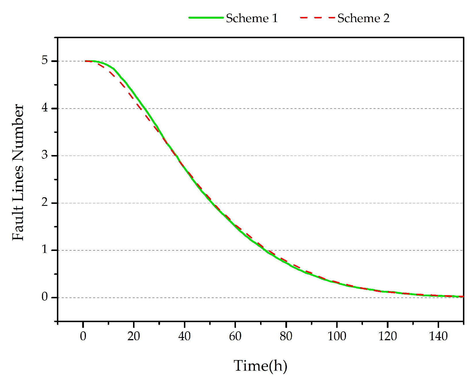
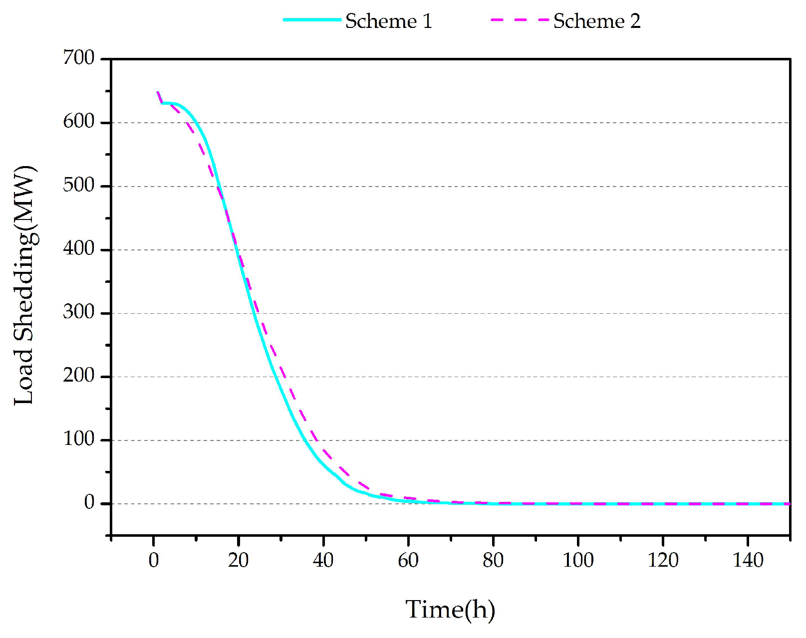
By analyzing the restoration process curves in Figure 6 and Figure 7, it can be found that in the initial stage of restoration, the amount of load shedding drops rapidly; this is because the DGs on nodes with load loss can take the lead in restoring important load, which improves the restoration efficiency. In the early stage of system restoration, the restoration speed of Scheme 2 is higher than that of Scheme 1, and the load shedding amount of Scheme 2 declines more sharply. While in the middle and later stages, the situation is just the opposite, which applies equally to the repair process of fault lines.
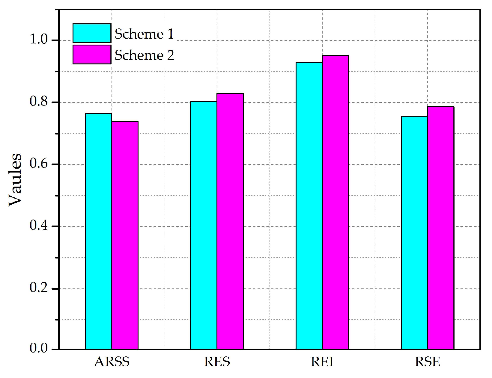
The above analysis also explains the reason why most restoration ability metrics of Scheme 2 are better, as shown in Figure 8. Although the restoration time of Scheme 1 is shorter and its ARSS is higher, the important and the sub-important load, with larger weight factors and economic loss factors, are firstly restored through Scheme 2. Therefore, the metrics of Scheme 2 perform better. For decision makers, if the loss of non-important load could be compensated in other ways under power market, Scheme 2 is undoubtedly the better restoration choice.
4. Conclusions
Resilience of power system has emerged as a novel concept to resist the damage from various disasters. The paper innovatively divided resilience assessment approaches under a tri-stage framework, in accordance with the process of disaster evolution: pre-disaster toughness, during-disaster resistance and post-disaster restoration ability. The proposed approaches were tested by the IEEE RTS 79 system. The main conclusions of the paper are as follows:
- In the pre-disaster stage, the robustness and toughness of power systems against specific disasters is analyzed. To demonstrate the expected risk and damage situation, some metrics are synthetically proposed, which can be obtained through the toughness assessment algorithm based on Monte Carlo Simulation. PMRM is firstly introduced in the field of resilience assessment, which enriches the metric system of toughness and provides more risk information for decision makers.
- In the during-disaster stage, the real-time resistance to disasters is the core to be emphasized, and SE is applied to estimate the states of components and power systems, in the case of measurement losses due to the destruction caused by disasters. According to the estimated results, flexible and effective dispatching and operation measures can be implemented to block the further spread of faults and mitigate the losses.
- In the post-disaster stage, the proposed assessment method can simulate the whole system restoration procedure, once the repair and restoration scheme is formulated. The response ability, the restoration ability and the restoration economic of power systems could be quantified by the related metrics, which provides adequate support for restoration strategies.
This assessment framework outlines the critical issues of each stage, enables the modelling of power system states against disaster, and quantifies the resilience of power systems precisely.
Author Contributions
H.Z., H.Y. and G.L. conceived and designed the study. H.Z. and H.Y. wrote the paper. Y.L. polished the paper.
Acknowledgments
This work was supported by the National Natural Science Foundation of China (51577147) and Science and Technology Project of State Grid, China (5202011600UG).
Conflicts of Interest
The authors declare no conflict of interest.
Abbreviations
| PMRM | Partitioned multi-objective risk method; |
| SE | State estimation; |
| SMCS | Sequential Monte Carlo Simulation; |
| LOLP | The loss of load probability; |
| EDNS | The expectation of demand not supplied; |
| ALRIL | Average load loss ratio in case of load curtailment; |
| PCFD | The probability of components failed during disaster; |
| PSI | The possibility of system islanding; |
| PIN | The possibility of isolated note; |
| GMA | The generation margins of areas; |
| TMTS | The transmission margin of transmission section; |
| CREV | The conditional risk expected values; |
| CLLP | Current load loss percent; |
| ATCS | The available transmission capacity of the section; |
| APDA | The active power deficiency of the area; |
| PLLP | Post-disaster load loss percent; |
| AFS | The average falling speed of the system performance; |
| LEDSR | The time length from the end of disaster (ted) to the start of load restoration (tsl); |
| RLRO | The ratio of load restored in one hour after tsl; |
| tsp | The time length from ted to when the load of system recovers to the specified proportion; |
| ARSS | The average restoration speed of system load; |
| RES | The restoration efficiency of system load; |
| REI | The restoration efficiency of the important load; |
| RSE | The economy of the restoration schemes. |
References
- Schneider, K.P.; Tuffner, F.K.; Elizondo, M.A.; Liu, C.C.; Xu, Y.; Ton, D. Evaluating the feasibility to use microgrids as a resiliency resource. IEEE Trans. Smart Grid 2017, 8, 687–696. [Google Scholar] [CrossRef]
- Li, L.; Zhang, Y. Analysis of major power outage events and implication on Chinese power system safe operation. China Power Enterp. Manag. 2014, 15, 16–18. (In Chinese) [Google Scholar]
- Panteli, M.; Trakas, D.N.; Mancarella, P.; Hatziargyriou, N.D. Power Systems Resilience Assessment: Hardening and Smart Operational Enhancement Strategies. Proc. IEEE 2017, 105, 1202–1213. [Google Scholar] [CrossRef]
- Berkeley, A.R.; Wallace, M. A Framework for Establishing Critical Infrastructure Resilience Goals; National Infrastructure Advisory Council (NIAC): Arlington, VA, USA, 2010. [Google Scholar]
- Cabinet Office. Keeping the Country Running: Natural Hazards and Infrastructure; Cabinet Office: London, UK, 2011. [Google Scholar]
- Panteli, M.; Mancarella, P. The grid: Stronger, bigger, smarter?: Presenting a conceptual framework of power system resilience. IEEE Power Energy Mag. 2015, 13, 58–66. [Google Scholar] [CrossRef]
- Panteli, M.; Mancarella, P. Influence of extreme weather and climate change on the resilience of power systems: Impacts and possible mitigation strategies. Electr. Power Syst. Res. 2015, 127, 259–270. [Google Scholar] [CrossRef]
- Fan, M.; Zeng, Z.; Zio, E.; Kang, R.; Chen, Y. A stochastic hybrid systems model of common-cause failures of degrading components. Reliab. Eng. Syst. Saf. 2018, 172, 159–170. [Google Scholar] [CrossRef]
- Chiacchio, F.; D’Urso, D.; Famoso, F.; Bruscac, S.; Aizpuruad, J.I.; Catterson, V.M. On the use of dynamic reliability for an accurate modelling of renewable power plants. Energy 2018, 151, 605–621. [Google Scholar] [CrossRef]
- Bie, Z.; Lin, Y.; Li, G.; Li, F. Battling the Extreme: A Study on the Power System Resilience. Proc. IEEE 2017, 105, 1253–1266. [Google Scholar] [CrossRef]
- Watson, J.-P.; Guttromson, R.; Monroy, C.S.; Jeffers, R.; Jones, K.; Ellison, J.; Rath, C.; Gearhart, J.; Jones, D.; Corbet, T.; Hanley, C.; Walker, L.T. Conceptual Framework for Developing Resilience Metrics for the Electricity, Oil, and Gas Sectors in the United States; Sandia National Laboratories (SNL): Albuquerque, NM, USA, 2014. [Google Scholar]
- Shinozuka, M.; Chang, S.E.; Cheng, T.C.; Feng, M.; O’Rourke, T.D.; Saadegbvaziri, M.A.; Dong, X.; Wang, Y.; Sbi, P. Resilience of integrated power and water systems. In Research Progress & Accomplishments; Multidisciplinary Center for Earthquake Engineering Research (MCEER): Buffalo, NY, USA, 2004. [Google Scholar]
- Chanda, S.; Srivastava, A.K. Defining and enabling resiliency of electric distribution systems with multiple microgrids. IEEE Trans. Smart Grid 2016, 7, 2859–2868. [Google Scholar] [CrossRef]
- Whitson, J.C.; Ramirez-Marquez, J.E. Resiliency as a component importance measure in network reliability. Reliab. Eng. Syst. Saf. 2009, 94, 1685–1693. [Google Scholar] [CrossRef]
- Maliszewski, P.J.; Perrings, C. Factors in the resilience of electrical power distribution infrastructures. Appl. Geogr. 2012, 32, 668–679. [Google Scholar] [CrossRef]
- Reed, D.A.; Kapur, K.C.; Christie, R.D. Methodology for assessing the resilience of networked infrastructure. IEEE Syst. J. 2009, 3, 174–180. [Google Scholar] [CrossRef]
- Panteli, M.; Pickering, C.; Wilkinson, S.; Dawson, R.; Mancarella, P. Power System Resilience to Extreme Weather: Fragility Modeling, Probabilistic Impact Assessment, and Adaptation Measures. IEEE Trans. Power Syst. 2016, 32, 3747–3757. [Google Scholar] [CrossRef]
- Wang, B.; Zhou, Y.; Mancarella, P.; Panteli, M. Assessing the impacts of extreme temperatures and water availability on the resilience of the GB power system. In Proceedings of the 2016 IEEE International Conference on Power System Technology (POWERCON), Wollongong, NSW, Australia, 28 September–1 October 2016. [Google Scholar]
- Liu, X.; Shahidehpour, M.; Li, Z.; Liu, X.; Cao, Y.; Bie, Z. Microgrids for Enhancing the Power Grid Resilience in Extreme Conditions. IEEE Trans. Smart Grid 2016, 8, 589–597. [Google Scholar] [CrossRef]
- Panteli, M.; Mancarella, P.; Trakas, D.N.; Kyriakides, E.; Hatziargyriou, N.D. Metrics and Quantification of Operational and Infrastructure Resilience in Power Systems. IEEE Trans. Power Syst. 2017, 32, 4732–4742. [Google Scholar] [CrossRef]
- Espinoza, S.; Panteli, M.; Mancarella, P.; Rudnicka, H. Multi-phase assessment and adaptation of power systems resilience to natural hazards. Electr. Power Syst. Res. 2016, 136, 352–361. [Google Scholar] [CrossRef]
- Subcommittee, P.M. IEEE Reliability Test System. IEEE Trans. Power Appar. Syst. 1979, PAS-98, 2047–2054. [Google Scholar] [CrossRef]
- Asbeck, E.; Haimes, Y.Y. The partitioned multiobjective risk method (PMRM). Large Scale Syst. 1984, 6, 13–38. [Google Scholar]
- Alvehag, K.; Soder, L. A Reliability Model for Distribution Systems Incorporating Seasonal Variations in Severe Weather. IEEE Trans. Power Deliv. 2011, 26, 910–919. [Google Scholar] [CrossRef]
- Li, G.; Zhang, P.; Luh, P.B.; Li, W.; Bie, Z.; Serna, C.; Zhao, Z. Risk Analysis for Distribution Systems in the Northeast U.S. Under Wind Storms. IEEE Trans. Power Syst. 2014, 29, 889–898. [Google Scholar] [CrossRef]
- Cadini, F.; Agliardi, G.L.; Zio, E. A modeling and simulation framework for the reliability/availability assessment of a power transmission grid subject to cascading failures under extreme weather conditions. Appl. Energy 2017, 185, 267–279. [Google Scholar] [CrossRef] [Green Version]
- Vishnu, T.P.; Viswan, V.; Vipin, A.M. Power system state estimation and bad data analysis using weighted least square method. In Proceedings of the 2015 IEEE International Conference on Power, Instrumentation, Control and Computing (PICC), Thrissur, India, 9–11 December 2015. [Google Scholar]
- Abur, A.; Exposito, A.G. Power System State Estimation Theory and Implementation, 1st ed.; Marcel Dekker, Inc.: New York, NY, USA, 2004; pp. 20–44. ISBN 20049780203913673. [Google Scholar]
- TRB Highway Capacity Manual. Special Report 209: Highway Capacity Manual, 3rd ed.; Transportation Research Board, National Research Council (NRC): Washington, DC, USA, 1994. [Google Scholar]
- London Economics International LLC. Estimating the Value of Lost Load. In Briefing Paper Prepared for the Electricity Reliability Council of Texas Inc.; London Economics International (LLC): Boston, MA, USA, 2013. [Google Scholar]
- Arab, A.; Khodaei, A.; Khator, S.K.; Han, Z. Electric Power Grid Restoration Considering Disaster Economics. IEEE Access 2016, 4, 639–649. [Google Scholar] [CrossRef]
Figure 1.
The illustrative process of a resilient power system under disasters.

Figure 2.
The simulation procedure for assessing system restoration ability.

Figure 3.
The system topology of the IEEE RTS 79 test system.

Figure 4.
Partial toughness assessment metrics results: (a) The results of EDNS and LOLP under different types of disasters; (b) The results of ALRIL and PCFD under different types of disasters; (c) The results of PIN and PSI under different types of disasters.
Figure 4.
Partial toughness assessment metrics results: (a) The results of EDNS and LOLP under different types of disasters; (b) The results of ALRIL and PCFD under different types of disasters; (c) The results of PIN and PSI under different types of disasters.

Figure 5.
CREV and condition probability for high and medium loss: (a) The PMRM assessment results for high loss; (b) The PMRM assessment results for medium loss.
Figure 5.
CREV and condition probability for high and medium loss: (a) The PMRM assessment results for high loss; (b) The PMRM assessment results for medium loss.

Figure 6.
Fault lines repair process.

Figure 7.
Load restoration process.

Figure 8.
Restoration efficiency and economic assessment results.


Table 1.
Scaling parameters.
| Parameter | Assigned Value |
|---|---|
| α | 113 |
| k | 4.60 |
| β | 3100 |
| μ | 40 |
Table 2.
Generation and transmission margins for toughness assessment.
| Metrics | Normal Condition | Typhoon | Lightning |
|---|---|---|---|
| GMA(Area 1) | −1.025110 | −1.008275 | −1.002412 |
| GMA(Area 2) | 0.852445 | 0.856448 | 0.855681 |
| TMTS | 1.017020 | 0.562210 | 0.524445 |
Table 3.
Toughness metrics under different wind speeds.
| Metrics | Normal | 30 m/s | 38 m/s | 52 m/s |
|---|---|---|---|---|
| EDNS(MW) | 14.799560 | 20.963996 | 27.547287 | 219.594647 |
| LOLP | 0.085200 | 0.111570 | 0.138480 | 0.630640 |
| TMTS | 1.017020 | 0.917633 | 0.562210 | 0.132837 |
| PSI | 0.000320 | 0.000750 | 0.005980 | 0.181280 |
Table 4.
The estimation errors of measurement loss with different orders.
| Order | Average Error | Median Error |
|---|---|---|
| The one-order loss | 5.32% | 3.68% |
| The two-order loss | 6.88% | 5.38% |
| The three-order loss | 8.34% | 9.09% |
Table 5.
The calculation results of two cases to further valid SE.
| Failure Mode | Estimated Power Flow | Actual Power Flow | Error | Estimated Power Flow | Actual Power Flow | Error |
|---|---|---|---|---|---|---|
| 12–13 (11–14) | P11-14 = −163.3 MW | P11-14 = −167.8 MW | 2.71% | P14-11 = 165.4 MW | P14-11 = 169.5 MW | 2.45% |
| 11–13 15–24 (12–23) | P12-23 = −273.8 MW | P12-23 = −278.5 MW | 0.77% | P23-12 = 286.4 MW | P23-12 = 288.6 MW | 1.72% |
Table 6.
The practical case of SE during disasters.
| Failure Mode | Estimated Power Flow | Actual Power Flow | Error | Estimated Power Flow | Actual Power Flow | Error |
|---|---|---|---|---|---|---|
| Before adjustment | P12-23 = −416.4 MW | P12-23 = −433.5 MW | 3.96% | P23-12 = 451.5 MW | P23-12 = 462.4 MW | 2.37% |
| After adjustment | P12-23 = −378.0 MW | P12-23 = −387.5 MW | 2.44% | P23-12 = 405.6 MW | P23-12 = 409.2 MW | 0.88% |
Table 7.
The output adjustment of generators.
| Bus Number | Output Adjustment |
|---|---|
| Bus 1 | +20 MW |
| Bus 2 | +20 MW |
| Bus 7 | +30 MW |
| Bus 13 | −81.2 MW |
Table 8.
The calculation result of during-disaster resistance.
| Metrics | Value |
|---|---|
| CLLP | 0 |
| ATCS (MVA) | 212.77 |
| APDA-Area 1 (MW) | 678 |
Table 9.
The distribution of load shedding.
| Bus Number | 1 | 5 | 6 | 8 | 10 |
|---|---|---|---|---|---|
| Load Curtailed (MW) | 75 | 71 | 136 | 171 | 195 |
Table 10.
The Information of DGs on important load.
| Bus Number | The Capacity of DG (MW) | The Time of Beginning to Operate (h) |
|---|---|---|
| 5 | 5 | 2 |
| 8 | 12 | 2 |
| 10 | 12 | 2 |
Table 11.
The locations of fault points.
| Line | 15–24 | 11–14 | 12–23 | 11–13 | 12–13 |
|---|---|---|---|---|---|
| Distance (km) | 70, 20, 15 | 55, 28 | 108, 3, 6, 48 | 75, 38, 4 | 90, 13, 4, 3 |
Table 12.
Losses assessment result.
| Metrics | PLLP | AFS |
|---|---|---|
| Values | 22.73% | 0.947%/h |
Table 13.
Scheme 1 for system restoration.
| Team | Task 1 | Task 2 |
|---|---|---|
| Team 1 | 18 (30, 38, 4) | 20 (65, 13, 4, 3) |
| Team 2 | 21 (108, 4, 48) | - |
| Team 3 | 27 (70, 20, 15) | 19 (110, 28) |
Table 14.
Scheme 2 for system restoration.
| Team | Task 1 | Task 2 |
|---|---|---|
| Team 1 | 19 (55, 28) | 18 (30, 38, 4) |
| Team 2 | 20 (90, 13, 4, 3) | 21 (58, 4, 48) |
| Team 3 | 27 (70, 20, 15) | - |
Table 15.
The response ability of the system.
| Metrics | Scheme 1 | Scheme 2 |
|---|---|---|
| LEDSR(h) | 2.25 | 2.25 |
| RLRO | 0.17 | 0.17 |
| tsp(h) | 16.25 | 15.25 |
© 2018 by the authors. Licensee MDPI, Basel, Switzerland. This article is an open access article distributed under the terms and conditions of the Creative Commons Attribution (CC BY) license (http://creativecommons.org/licenses/by/4.0/).
Share and Cite
MDPI and ACS Style
Zhang, H.; Yuan, H.; Li, G.; Lin, Y. Quantitative Resilience Assessment under a Tri-Stage Framework for Power Systems. Energies 2018, 11, 1427. https://doi.org/10.3390/en11061427
AMA Style
Zhang H, Yuan H, Li G, Lin Y. Quantitative Resilience Assessment under a Tri-Stage Framework for Power Systems. Energies. 2018; 11(6):1427. https://doi.org/10.3390/en11061427
Chicago/Turabian StyleZhang, Han, Hanjie Yuan, Gengfeng Li, and Yanling Lin. 2018. "Quantitative Resilience Assessment under a Tri-Stage Framework for Power Systems" Energies 11, no. 6: 1427. https://doi.org/10.3390/en11061427
Note that from the first issue of 2016, this journal uses article numbers instead of page numbers. See further details here.