Robust Smart Meter Data Analytics Using Smoothed ALS and Dynamic Time Warping

Abstract

This paper presents a robust data-driven framework for clustering large-scale daily chronological load curves from smart meters, with a focus on the challenges encountered in practice. The first challenge is the low data quality issue due to bad and missing data, which has been a major obstacle for various in-depth analyses of smart meter data. A novel Smoothed Alternating Least Squares (SALS) approach is proposed to recover missing/bad smart meter data by taking advantage of their low-rank property. The second challenge is brought by different data reporting rates of smart meters. A Dynamic Time Warping (DTW)-based approach is proposed that is more efficient and eliminates the need for data interpolation or measurement downsampling. The proposed approach enables flexible data collection strategies and gateway locations to meet various smart grid performance requirements. The proposed framework is tested through experiments using real-world smart meter data.

1. Introduction

The widespread deployment of smart meters (SMs) has made available a huge amount of energy consumption information from individual customers as well as aggregated communities. By enabling two-way communication between utilities and customers, SMs become a critical component of smart grids. SMs allow utilities to monitor every energy delivery point of their networks from once per month to every 5–15 min [1,2], a 3000-fold increase in data volume. For utilities, this opens up new opportunities, allowing them to do things they never could before. Data gathered from smart meters can provide a better understanding of customer segmentation, behavioral patterns, dynamic electricity pricing strategies, etc.

In practice, during the process of collection and transmission, data corruption and missing problems occur quite often, which can be caused by equipment malfunction, communication failure, extreme weather conditions, etc. In addition, smart meters from different regions, vendors, and utilities can be set to report at different rates, which complicates analysis and applications based on large-scale smart meter data. Although these issues have been reported in the existing literature, few works have been conducted to explicitly address the challenges associated with various smart meter data analytic applications.

The problem of missing data is relatively common in practice and can have a significant effect on the conclusions drawn. In general, data imputation can help by replacing missing data with estimated values. Data imputation improves the accuracy of forecasting, enhances data analysis, and facilitates decision-making, etc. Conventional data imputation methods include linear interpolation, mean (median) substitution, hotdeck imputation (using the last observed values as estimates in an ordered dataset), and regression imputation [3,4]. These approaches gain popularity in many data mining and machine learning applications due to their computational efficiency, with time complexity O(n) the most popular. However, a major downside of these approaches is their lower accuracy, and biased estimates are often expected. In [5], nonparametric regression methods are proposed to cleanse corrupted and missing load curve data of smart meters. However, the performance depends on human interference with the smoothness level, which significantly limits the applications of such approaches. The authors of [6] propose using a weighted average combination of historical data to impute missing smart meter data, but unfortunately the performance of this approach is not explicitly discussed. Due to the limits of traditional methods, solving the missing data or matrix completion problems through matrix decomposition has become more popular recently.

On the other hand, depending on data collection strategies and gateway locations, SMs can have vastly different reporting rates across different regions [7]. These scenarios are typically referred to as imbalance class distribution in data science. Data interpolation and downsampling (or subsampling) are usually utilized to address the challenges, but research has shown that they could lead to biased and inaccurate results. For example, machine learning algorithms tend to produce unsatisfactory classifiers when faced with imbalanced datasets.

In distribution networks, the categorization or clustering of load profiles (or load curves, used interchangeably in this paper) is important to utilities and their customers. Utilities can take advantage of the categorized load curves for demand side management, fluctuation smoothing, load leveling, and load forecasting. In addition, customers can participate in the competitive electricity market by using a demand-side bidding mechanism utilizing energy storage systems or by proper tariff selection [8].

To conduct load clustering, the time series load curves of year, season or month can be used. Over the past few years, much research has been put into load curves classification in order to solve the short-term load forecasting of anomalous days and identify different types of customers and their behaviors. Clustering methods that have been discussed so far are the self-organizing map, the k-means, the fuzzy k-means, and the average and Ward hierarchical methods [9,10,11]. These methods generally belong to pattern recognition techniques [12]. Alternatively, the customer classification problem can be solved by using data mining, frequency-domain data [11,12], etc. The most commonly used respective adequacy measures are the mean index adequacy, the clustering dispersion indicator, the similarity matrix indicator, the Davies-Bouldin indicator, the modified Dunn index, the scatter index, and the mean square error [13].

Generally speaking, the aforementioned approaches assume that the smart meter (load) data all have the same sampling rate. However, in practice, SMs from different regions, vendors, and utilities can be set to report at different rates, which complicates analysis and applications based on large-scale smart meter data. These scenarios are typically referred to as imbalance class distribution in data science. Data interpolation and downsampling (or subsampling) can be easily implemented to work around problems, but research has shown that they could lead to biased and inaccurate results. For example, machine learning algorithms tend to produce unsatisfactory classifiers when faced with imbalanced datasets. To address this challenge, a novel dynamic time warping (DTW)-based multivariate time series classification approach is proposed for large-scale smart meter data analysis.

In this paper, the aforementioned challenges are addressed with an innovative robust smart meter data analytic framework. First, a novel data imputation algorithm, smoothed alternating least squares (SALS), is proposed to recover missing and corrupted data for large-scale smart meter dataset. Different from conventional data imputation approaches, SALS recovers missing values by learning the spatial–temporal properties of data and make inference, which improves the estimation accuracy. Second, a novel data-driven approach based on dynamic time warping (DTW) is proposed to cluster large-scale daily chronological load curves with different sampling rates. Using the proposed approach, smart meter data are warped non-linearly in the time dimension to determine a measure of their similarity independent of certain non-linear variations in the time dimension. Experimental results using real-world smart meter data demonstrate the effectiveness and advantages of the proposed framework.

2. Missing and Bad Data Recovery

In practice, missing or bad data recovery can usually be converted into a matrix completion problem. In this section, the matrix completion problem is introduced first and the data missing problem is formulated as a matrix completion problem based on its low-rank property.

2.1. Matrix Completion Problem

Matrix completion refers to the task of filling in the missing entries of a partially observed matrix. Matrix completion aims at filling in the missing entries of a matrix based on observed entries. Without any assumption, matrix completion would be random guessing, which would be meaningless. Consequently, in most cases, a matrix completion task assumes the target matrix to be of low rank and seeks the lowest rank complete matrix [14]. The low-rank assumption guarantees that the complete matrix will be a linear combination of a lower rank matrix, and that the low-rank basis will reflect the common pattern of data.

Let $M=\left\{m_{ij}\right\}\in {ℝ}^{n_1\times n_2}$ be the matrix with missing values, $X=\left\{x_{ij}\right\}\in {ℝ}^{n_1\times n_2}$ be the matrix to be completed, and $\mathsf{\Omega }=\left\{\left(i,j\right)|m_{ij}\mathrm{is}\mathrm{observed}\right\}$ is observed. The objective function for the matrix completion problem can be then summarized as follows:

$$\begin{gathered} \underset{X}{\min }\mathrm{rank}\left(X\right), \\ s.t. {{\displaystyle \sum }}_{\left(i,j\right)\in \mathsf{\Omega }}{\left(x_{ij}-m_{ij}\right)}^2\le \epsilon \end{gathered}$$

(1)

where ε is a parameter that limits the training error. In the objective function, we expect to find the minimum rank complete matrix whose entries in $\mathsf{\Phi }$ are close to the observed entries in the target matrix. In general, the above problem is hard to solve because of the rank constraint [15]. Consequently, a slight modification of the original objective function is used to simplify the computation.

$$\begin{gathered} \underset{X}{\min }\Vert X\Vert , \\ s.t. {{\displaystyle \sum }}_{\left(i,j\right)\in \mathsf{\Omega }}{\left(x_{ij}-m_{ij}\right)}^2\le \epsilon , \end{gathered}$$

(2)

where ‖X‖ denotes the Euclidean norm, or the sum of singular values of X. It has been proven under many conditions that the Euclidean norm is an effective convex relaxation to the rank constraint [16,17,18]. Equation (2) is a semi-definite programming problem and can be solved with optimization software like SeDuMi. However, those algorithms are computationally expensive, as the data size is typically very large for the matrix completion problems. Note that, at this point, minimizing ‖X‖ while constraining ${{\displaystyle \sum }}_{\left(i,j\right)\in \mathsf{\Omega }}{\left(x_{ij}-m_{ij}\right)}^2$ are essentially the same problem as minimizing ${{\displaystyle \sum }}_{\left(i,j\right)\in \mathsf{\Phi }}{\left(x_{ij}-m_{ij}\right)}^2$ while restraining ‖X‖. Therefore, the optimization problem can further be reformulated as follows:

$$\begin{gathered} \underset{X}{\min }{{\displaystyle \sum }}_{\left(i,j\right)\in \mathsf{\Omega }}{\left(x_{ij}-m_{ij}\right)}^2 \\ s.t. \Vert X\Vert \le {\epsilon }^{\prime } \end{gathered}$$

(3)

Equation (3) is a convex optimization problem that satisfies Slater’s condition [19]. Specifically, for any given ${\epsilon }^{\prime }$, there exists a matrix X = 0 in the feasible region, such that strict feasibility holds, $\Vert X\Vert \le {\epsilon }^{\prime }$. Therefore, strong duality holds and its Lagrangian form can be utilized to solve the problem.

$$\underset{X}{\min }{{\displaystyle \sum }}_{\left(i,j\right)\in \mathsf{\Omega }}{\left(x_{ij}-m_{ij}\right)}^2+\lambda \Vert X\Vert$$

(4)

Instead of solving for Equation (2), most matrix completion problems use Equation (4) as the objective function for the convex structure and the provable near-optimal solution. There are multiple methods to optimize Equation (4); one of the most commonly used methods is by matrix factorization. Matrix factorization attempts to find the low-rank approximation of X by computing the matrix decomposition X = A^TB, where $A=\left[a_1,a_2,\dots ,a_{n1}\right]\in {ℝ}^{k\times n1}$ and $B=\left[b_1,b_2,\dots ,b_{n2}\right]\in {ℝ}^{k\times n2}$, and k < min(n₁, n₂). The objective function can be transformed via:

$$\underset{A, B}{\min }{{\displaystyle \sum }}_{\left(i,j\right)\in \mathsf{\Omega }}{\left(a_i^T{b}_j-m_{ij}\right)}^2+\lambda \Vert A^{T}B\Vert$$

(5)

It has been proved in [20] that

$$\Vert X\Vert =\underset{A,B:X=A^{T}B}{\min }\frac{1}{2}\left({\Vert A\Vert }^2+{\Vert B\Vert }^2\right)$$

(6)

Equation (5) can be reformulated as:

$$\underset{A, B}{\min }{{\displaystyle \sum }}_{\left(i,j\right)\in \mathsf{\Omega }}{\left(a_i^T{b}_j-m_{ij}\right)}^2+\lambda \left({\Vert A\Vert }^2+{\Vert B\Vert }^2\right)$$

(7)

Equation (7) is an intimate approximation of Equation (4), and the method known as maximum margin matrix factorization (MMMF) [21] uses Equation (7) as objective function to find the near-optimal complete matrix. Mardani et al. [22] prove that Equation (7) does not suffer any loss of optimality relative to Equation (4). Additionally, [23] proves that the solution of MMMF is capable of recovering matrices with missing entries.

In general, the core idea of matrix completion is that the data matrix is a linear combination of a lower rank matrix. Typically, Alternating Least Squares (ALS) is used to solve the matrix completion problem by implementing low-rank matrix decomposition. In particular, it assumes that there are certain patterns in the data, and that these patterns are described in a low-rank matrix. The low-rank assumption matches the nature of the load curve data from smart meters, i.e., the load curve data usually follow a certain fixed pattern. Under the smart meter data recovery setting, it is assumed that there is a set of typical daily load curves on which the entire matrix can be rebuilt through linear combination.

2.2. Alternating Least Squares (ALS)

ALS is implemented to solve the maximum margin matrix factorization (MMMF) problem. Note that the objective function of Equation (7) is not convex because of the $a_i^T{b}_j$ term. In this case, ALS optimizes the objective function in an alternating fashion, i.e., fix A and optimize B; then fix B and optimize A. Note that if A (or B) is fixed, the objective is a convex function of B (or A). Even more conveniently, when A is fixed and regarded as a constant, Equation (7) is of quadratic form in terms of B. Consequently, the near-optimal solution can be obtained through simple linear algebra derivation. Taking advantage of this property, ALS optimizes A and B in an alternating fashion, and the result is guaranteed to converge to a local optimum. More specifically, the ALS algorithm can be summarized as follows (Algorithm 1) [24]:

Algorithm 1. Alternating Least Squares.

Input: Matrix M, rank of decomposition k

Output: Matrix X, X = ATB

Randomly initialize matrix A and B

whilenot convergedo

for i = 1,2, …, n1 do

$a_i={\left({\displaystyle {\displaystyle \sum }_{j:\left(i,j\right)\in \mathsf{\Omega }}}{b}_j{b}_j^T+\lambda I_k\right)}^{-1}{\displaystyle {\displaystyle \sum }_{\left(i,j\right)\in \mathsf{\Omega }}}{m}_{ij}{b}_j$

end for

for j = 1, 2, …, n2 do

$b_j={\left({\displaystyle {\displaystyle \sum }_{\left(i,j\right)\in \mathsf{\Omega }}}{a}_i{a}_i^T+\lambda I_k\right)}^{-1}{\displaystyle {\displaystyle \sum }_{\left(i,j\right)\in \mathsf{\Omega }}}{m}_{ij}{b}_i$

end for

end while

As discussed above, matrix A and B are updated in an alternating fashion. In each iteration, a_i’s are first updated based on existing values of b_j’s, and then b_j’s are evaluated with the updated values of a_i’s. It is worth mentioning that to update values in a_i, only part of matrix B, corresponding to the observed set on the ith row, is used. The same rule applies when updating matrix B.

The observed entry values m_ij are used in each update. An intuitive interpretation of this algorithm is that matrices A and B are updated according to the observed entries so that A^TB is as close to M on the observed set as possible. Moreover, because of the low-rank assumption, patterns of M are learned on the observed entries and stored in matrices A and B. Therefore, after getting the pattern of the data and approximating observed entries, ALS can efficiently recover missing values on the missing entries.

The convergence condition needs to be able to terminate the algorithm when little or no update is made from the previous iteration. Currently, we use the Mean Absolute Error (MAE) on the observed set as the criterion, i.e., when the difference between the MAE of previous and current iteration is smaller than a certain threshold, we then assume that the algorithm has converged and terminate the algorithm.

2.3. Smoothed Alternating Least Squares (SALS)

In this work, we improve ALS by proposing an algorithm that is more suitable for time-series data, Smoothed Alternating Least Squares (SALS). In the ALS model, matrix B corresponds to the lower rank basis, and matrix A is the coefficient matrix. Rows in matrix B can be considered the typical daily load curves, and it is assumed that columns of B are independent. However, for daily load curves, the columns of data are not independent. More specifically, it is expected that the load curves should be smooth and show continuous patterns. Such an assumption in the ALS model can be interpreted as the need for rows in matrix B to be smooth instead of volatile.

Based on this assumption, we propose a smoothness regularization term in the objective function. Specifically, the new objective function is defined as follows:

$$\underset{A, B}{\min }{{\displaystyle \sum }}_{\left(i,j\right)\in \mathsf{\Omega }}{\left(a_i^T{b}_j-m_{ij}\right)}^2+\lambda \left({\Vert A\Vert }^2+{\Vert B\Vert }^2\right)+\mu {{\displaystyle \sum }}_{k=1}^{n_2-1}\Vert b_k-b_{k+1}\Vert {}^2$$

(8)

The regularization term $\mu {{\displaystyle \sum }}_{k=1}^{n2-1}\Vert b_k-b_{k+1}\Vert {}^2$ penalizes if rows in B are unstable, and µ controls how much to penalize the instability. Notice that with the new regularization term, the objective function is still convex in terms of b_j’s after fixing A. Therefore, the general algorithm in ALS is still valid for the new objective function. What is needed to be modified is just how to update b_j’s.

When B is fixed, gradients of ai in Equation (8) are identical to those in Equation (7), as the new regularization term does not affect A. Consequently, SALS updates a_i’s the same way as ALS. As for when A is fixed, the expression to update b_j imsub:

$$\frac{\partial X}{\partial b_j}={{\displaystyle \sum }}_{i:\left(i,j\right)\in \mathsf{\Omega }}2\left(a_i{a}_i^T{b}_j-m_{ij}{a}_i\right)+2\lambda b_j+\mu \left(4b_j-2b_{j+1}-2b_{j-1}\right)$$

(9)

Equation (9) uses the fact that the 2-norm of a matrix is the root of summation of all the squared entry values, i.e., ${\Vert A\Vert }^2={{\displaystyle \sum }}_{\left(i,j\right)}{a}_{ij}^2={{\displaystyle \sum }}_i\Vert a_i\Vert {}^2$. In Equation (9), represents the new objective function, Equation (8). The optimum is obtained when Equation (9) equals 0, which gives the following:

$$\left({{\displaystyle \sum }}_{i:\left(i,j\right)\in \mathsf{\Omega }}{a}_i{a}_i^T+\lambda I_k+2\mu I_k\right)b_j-{{\displaystyle \sum }}_{i:\left(i,j\right)\in \mathsf{\Omega }}{m}_{ij}{a}_i-\mu b_{j+1}-\mu b_{j-1}=0$$

(10)

and, further,

$$b_j={\left({{\displaystyle \sum }}_{i:\left(i,j\right)\in \mathsf{\Omega }}{a}_i{a}_i^T+\lambda I_k+2\mu I_k\right)}^{-1}\left({{\displaystyle \sum }}_{i:\left(i,j\right)\in \mathsf{\Omega }}{m}_{ij}{a}_i+\mu b_{j+1}+\mu b_{j-1}\right)$$

(11)

for 1 < j < n₂.

Equation (11) gives the expression to update b_j when 1 < j < n₂. Based on the above derivations, SALS can be summarized in the steps shown below (Algorithm 2).

Algorithm 2. Smoothed Alternating Least Squares.

Input: Matrix M, rank of decomposition k

Output: Matrix X, X = ATB

Implement k-means on rows of M that does not contain missing values

Initialize matrix B with k-means cluster centers

whilenot convergedo

for i = 1, 2, …, n1 do

$a_i={\left({\displaystyle {\displaystyle \sum }_{j:\left(i,j\right)\in \mathsf{\Omega }}}{b}_j{b}_j^T+\lambda I_k\right)}^{-1}{\displaystyle {\displaystyle \sum }_{j:\left(i,j\right)\in \mathsf{\Omega }}}{m}_{ij}{b}_j$

end for

$b_1={\left({\displaystyle {\displaystyle \sum }_{i:\left(i,1\right)\in \mathsf{\Omega }}}{a}_i{a}_i^T+\left(\lambda +\mu \right)I_k\right)}^{-1}\left({\displaystyle {\displaystyle \sum }_{i:\left(i,1\right)\in \mathsf{\Omega }}}{m}_{i1}{a}_i+\mu b_2\right)$

for j = 1,2, …, (n2 − 1) do

$b_j={\left({\displaystyle {\displaystyle \sum }_{i:\left(i,j\right)\in \mathsf{\Omega }}}{a}_i{a}_i^T+\left(\lambda +2\mu \right)I_k\right)}^{-1}\left({\displaystyle {\displaystyle \sum }_{i:\left(i,j\right)\in \mathsf{\Omega }}}{m}_{ij}{a}_i+\mu \left(b_{i+1}+b_{i-1}\right)\right)$

end for

$b_{n_2}={\left({\displaystyle {\displaystyle \sum }_{i:\left(i,1\right)\in \mathsf{\Omega }}}{a}_i{a}_i^T+\left(\lambda +\mu \right)I_k\right)}^{-1}\left({\displaystyle {\displaystyle \sum }_{i:\left(i,m\right)\in \mathsf{\Omega }}}{m}_{i{n}_2}{a}_i+\mu b_{n_2-1}\right)$

end while

In SALS, the initialization is modified to improve the accuracy and convergence rate. The alternating update does not guarantee convergence to the global optimum, which makes the initialization even more crucial. Specifically, the k-means clustering step divides the n rows of data into k groups, and each group has a cluster center, which forms a center matrix of size k-by-n₂.

$$C=\left[\begin{array}{ccc}{c}_{1,1}& \cdots & c_{1,n_2}\\ ⋮& \ddots & ⋮\\ c_{k,1}& \cdots & c_{k,n_2}\end{array}\right]\in {ℝ}^{k\times n_2}$$

(12)

Rows of matrix C correspond to cluster centers. Then, matrix B is initialized with C, i.e., B = C.

To specify the initial model, it suffices to give either the initial matrix A or matrix B. For the proposed initialization scheme, matrix B is chosen to be initialized. As mentioned at the beginning of this subsection, rows in matrix B can be considered as typical daily load curves. It has been shown in [25] that k-means can efficiently extract typical load curves from smart meter data. Therefore, initializing matrix B with k-means cluster centers is able to improve the convergence rate.

Specifically, each row of the partially observed matrix M is rebuilt with a linear combination of B, i.e.,

$$M_i\approx a_i^{T}B$$

(13)

where M_i is the ith row of matrix M. Therefore, a good initialization of B should be able to approximate rows of M through linear combination.

If the data are properly clustered, each row of data matrix would be close to its corresponding cluster center, i.e., $\exists ts.t.B_t=C_t\approx M_j,\forall M_j$ without missing values, where C_t is the tth row of matrix C. In this case, each row of M is approximated by one row from B. Thus, k-means initialization can provide a decent start for the algorithm.

Another reason to modify the initialization process is that the proposed algorithm is better suited for the smoothness regularization term. In SALS, the turbulence of the curve is penalized based on the difference of adjacent b_j’s. Therefore, in each iteration, columns of matrix B are updated according to their adjacent columns to make the columns closer to their adjacency. The initial curves from k-means initialization are much smoother because of the nature of the load curve data, i.e., c_i,j is close to c_i,j+1 and c_i,j−1. In this case, updating columns of B according to their nearby columns can be much more helpful. However, the initial curves from random initialization are completely random. Points in these curves are far from adjacent points and, more importantly, they are independent. In this case, making the columns closer to their adjacent columns would not improve the results.

Compared with a random start, k-means initialization utilizes information from data to improve the convergence rate and estimation accuracy. For load curve data, curves defined by rows of matrix B become smooth after several iterations, even with a random start. In addition, in terms of accuracy the simulation results indicate that k-means initialization greatly outperforms random initialization.

In terms of computational cost, the time complexity for updating a_i in each iteration is O(n₂k + k²). Specifically, we have O(n₂k) for matrix multiplication and summation, and O(k²) for matrix inversion. Consequently, updating a_i, i = 1, …, n₁ takes O(n₁n₂k + n₁k²). A similar deduction goes for b_j’s until eventually we have the overall computational cost for SALS as O(n₁n₂k + (n₁ + n₂)k²).

3. DTW-Based Load Profile Classification

In a time series analysis, DTW is one of the algorithms for measuring the similarity between two temporal sequences that may vary in speed. For instance, similarities in walking could be detected using DTW, even if one person was walking much faster than the other, or if there were accelerations and decelerations during the course of an observation. DTW has been applied to temporal sequences of video, audio, and graphic data—indeed, any data that can be turned into a linear sequence can be analyzed with DTW. In general, DTW is a method that calculates an optimal match between two given sequences (e.g., time series) with certain restrictions. The sequences are warped non-linearly in the time dimension to determine a measure of their similarity independent of certain non-linear variations in the time dimension. This sequence alignment method is often used in time series classification.

Consider two load curves from SMs x_p = {x_p1, x_p2, x_p3, …, x_pi} and x_q = {x_q1, x_q2, x_q3, …, x_qk} estimated over the same time period, where i and k are numbers of data points for smart meter p and q, respectively. Number i and k can be equal, when both meters have the same reporting rate, or unequal when they have a different reporting rate.

A local distance measure d(x_pm, x_qn) of data points m and n from load curves x_p and x_q respectively is defined as:

$$d\left(x_{pm},x_{qn}\right)=\Vert x_{pm},x_{qn}\Vert {}^2$$

(14)

where m $\in$ {1, 2, 3, …, i} and n $\in$ {1, 2, 3, …, k}. Similarly, a distance matrix D(x_p, x_q) of size i-by-k is constructed by calculating local distance measures of each pair of data points from trajectories x_p and x_p.

Define w = {w₁, w₂, w₃, …, w_L} as a warping path, where w_l = (m_l, n_l) $\in$ [1:i] × [1:k] represents the cell in the m_lth row, n_lth column of a distance matrix D(x_p, x_q). A valid warping path as shown in Figure 1 satisfies the following conditions:

(1)

Boundary condition: w₁ = (1, 1) and w_L = (i, k). This condition ensures that the warping path starts and ends at diagonally opposite corner cells of the distance matrix D(x_p, x_q).

(2)

Continuity: if w₁ = (a, b) and w_l−1 = (a’, b’), a − a’ ≤ 1 and b − b’ ≤ 1. This condition restricts the feasible warping path to only adjacent cells.

(3)

Monotonicity: if w_l = (a, b) and w_l−1 = (a’, b’), a − a’ ≥ 0 and b − b’ ≥ 0. This condition ensures the path in w is made monotonically.

The total distance d_w(x_p, x_q) of a warping path w is defined as:

$$d_w\left(x_p,x_q\right)={{\displaystyle \sum }}_{l=1}^{L}d\left(x_{p{m}_l,}{x}_{q{n}_l}\right)$$

(15)

The DTW distance between two trajectories x_p and x_q is defined as the minimum total distance among all possible warping paths, which can be found by dynamic programming.

$$d_w\left(x_p,x_q\right)={{\displaystyle \sum }}_{l=1}^{L}d\left(x_{p{m}_l,}{x}_{q{n}_l}\right)=\min \left\{d_w\left(x_p,x_q\right)\right\}$$

(16)

where w is a warping path.

Using DTW with this warping path as a similarity measure, the clusters of load curves with similar shape are constructed regardless of stretching and contracting of the time axes. In this paper, the similarity between smart meter data p and q is represented by DTW(δ_p, δ_q). This allows a non-linear mapping between load curves, even with data loss or communication delays. DTW is highly ranked in pattern recognition and computer vision fields. It has been widely used in time series analysis, (partial) shape matching, speech recognition, and online signature verification. In [26], DTW is tested against Euclidean distance for small data size and is found to provide a smaller out-of-sample error rate as a result of its improved similarity measure [27].

Using DTW as a distance or similarity measure, clustering approaches including k-means, k-shape, and fuzzy k-means can be employed to classify load profiles. Given a set of n smart meter data (x₁, x₂, …, x_n), the objective of the load clustering problem is to classify loads into k (k ≤ n) clusters, denoted by S = {S₁, S₂, …, S_k}, so that the sum of all distances between each load and its corresponding centroid $\mu$’s is minimized, defined as:

$$\arg \min {{\displaystyle \sum }}_{i=1}^k{{\displaystyle \sum }}_{x\in S_i}{d}_w\left(x,{\mu }_i\right)$$

(17)

The DTW-based clustering algorithm can be started with a random initialization of the cluster centers. Or, as has been observed, by carefully selecting the initial seeds and supervising the clustering process, the limitations of existing clustering algorithm can be overcome and better clustering results can be obtained, e.g., by following the k-means++ algorithm [28]. In the assignment step, each load curve is assigned to the closest cluster based on $d_w\left(x_p,x_q\right)$. After finding the cluster membership of all load curves, the centroid ${\mu }_k$ of each cluster S_k can be updated, which is the minimizer of the sum of $d_w\left(x,{\mu }_k\right)$ over all x within cluster k.

The performance of the clustering can be calculated as the sum of squared error (SSE) in a recursive way based on dynamic programming, which determines the optimal comparison path. Assuming a total of N_c clusters are obtained with each cluster represented by S_t (t = 1, 2, …, N_c), the SSE is calculated as:

$$SSE={{\displaystyle \sum }}_{t=1}^{N_c}{{\displaystyle \sum }}_{x_j^{\left(t\right)}\in S_t}\Vert x_j^{\left(t\right)}-{\mu }^{\left(t\right)}\Vert$$

(18)

where $x_j^{\left(t\right)}$ is the location of load j, which belongs to cluster S_t, and ${\mu }^{\left(t\right)}$ is the centroid of cluster S_t.

4. Load Forecasting Based on Load Classification

The proposed load classification results for daily chronological load curves can be used in load forecasting. First of all, they can be used to improve the accuracy of the total system load forecast. Based on the historical clustering results of daily load curves as well as date type (four seasons and day of the week), area central heating season, temperature, and precipitation, we can forecast the load curve shape for a future day. Second, it can be used to improve the accuracy of bus load forecast. Bus load curve is calculated based on the total system load and the ratios among the distribution of system, substation, transformer, and bus. The number of groups from system to bus determines the accuracy of the bus load curve forecast. The clustering results of daily system load can be used to determine the distribution ratio and enhance the accuracy of the bus load forecast.

The proposed shape-based clustering results can also be applied to develop time of use (TOU) strategies. As a demand response method, utilities in some areas have adopted time of use strategies, and assign different prices based on the power system’s operational costs. The shape-based clustering results provide important information to determine the peak and off-peak prices for different seasons and days of the week. For example, if there are three different load curves in the summer, we can develop three different pricing plans for summer weekdays and summer weekends based on the different duration and peak times.

5. Experimental Results

The proposed algorithm is tested on a real-world smart meter dataset containing 1372 smart meters from an industrial county in China. Each observation in the dataset is a daily load profile and the total number of observations is 557,361. The time span of the dataset is four years, from 2011 to 2014, with a time interval of 15 min. However, a significant portion of the data is missing or corrupted, which explains why the number of actual data observations is much less than 365 × 4 × 1372 = 2,003,120.

The average load for the entire dataset is approximately 0.2 megawatt (MW). It is noted that about 4% of the data are missing in the dataset, and the data are usually missing in blocks, i.e., missing values appear consecutively. A total of 10 smart meters’ load curves, selected randomly, are shown in Figure 2.

As shown in the plot, the amplitudes vary significantly for different load curves with noise observed. Nevertheless, it can be observed that there are some patterns in the data; the curves are not completely random. Essentially, the proposed approach explores these patterns, which makes the load curve matrix low rank.

To validate the proposed approach and demonstrate its advantages, SALS is implemented and tested using smart meter load curve data. In addition, two existing model-based algorithms, random forest imputation (RF imputation) and k-NN imputation, are implemented on the same set of data and their performances in term of both accuracy and computation time are compared with the proposed one.

To evaluate the performance of algorithms, implementing the models on the entire dataset in a single simulation is not convincing, and the stability of the algorithm cannot be evaluated. Consequently, for the case studies, random subsamples of dataset are drawn multiple times to study the performance of algorithms from multiple simulations. For experiment and comparison purposes, missing data are also selected randomly.

In order to quantify the accuracy of different algorithms in terms of missing data recovery, the mean average error (MAE) is defined as the metric, as shown in Equation (19). Let $X^{*}=\left\{x_{ij}^{*}\right\}$ be the original smart meter data matrix, $X=\left\{x_{ij}\right\}$ be the recovered complete data matrix, and ${\mathsf{\Omega }}^{*}$ be the set of observed but erased entries.

$$MAE={\displaystyle \sum }_{\left(i,j\right)\in {\mathsf{\Omega }}^{*}}\Vert x_{ij}^{*}-x_{ij}\Vert /\left|{\mathsf{\Omega }}^{*}\right|$$

(19)

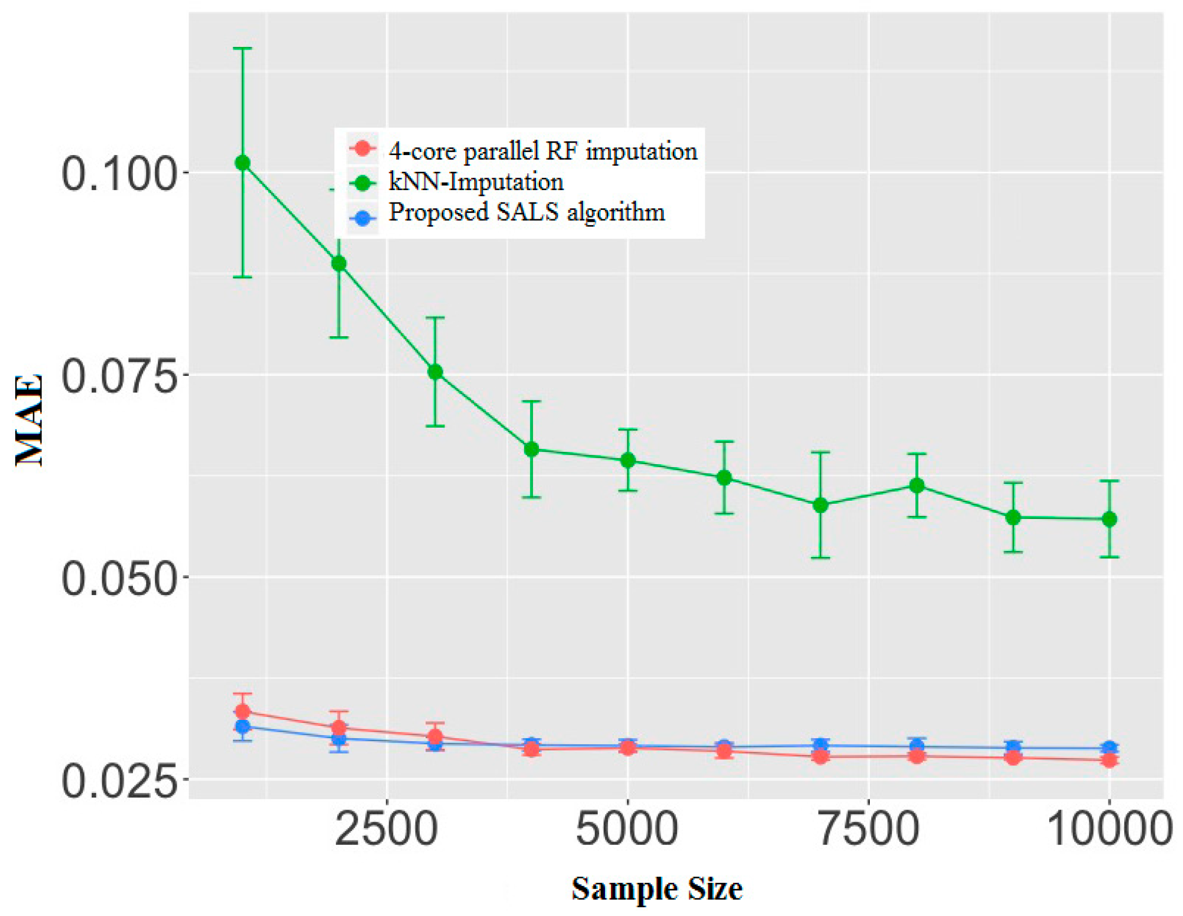
Figure 3 shows the accuracy comparison of the proposed SALS algorithm, k-NN imputation method, and 4-core paralleled RF imputation. Lines and error bars in the plot represent the means and standard deviations, respectively, of estimates from the 10 different experiments, each with a different sample size. We adopt the R library DMwR version of k-NN imputation and the missForest version of RF imputation. As for the k-NN imputation, based on multiple simulation results, the number of the nearest neighbor is chosen as 2 + n/1000. In addition, for the RF imputation model, the number of iterations is five, and the number of trees is 12. As the figure shows, in terms of accuracy, both RF imputation and SALS significantly outperform k-NN imputation. The accuracy of RF imputation and SALS is pretty close, although RF imputation demonstrates a slightly better ability to learn the pattern as the sample size grows. Nevertheless, the learning ability and recovery accuracy of RF imputation come at a great computational cost, as discussed below.

Figure 4 shows the computation time required to fully recover the missing data in the aforementioned dataset. Note that for the RF imputation approach, 4-core parallel computing is implemented to speed up the process. It is noted that RF imputation is highly parallelizable, since it builds a random forest model for each of the columns and these models are completely independent. As a result, implementing 4-core parallel computing can reduce the computational time by nearly 4-fold. However, as indicated in the plot, the computational time needed for random forest is still more than 10 times that required for the proposed SALS algorithm. As a comparison, the computation time required for the k-NN imputation approach also increases significantly as the number of data samples increases. The proposed approach takes the least computation time compared to the other two approaches. In addition, as the sample size increases, the computation time required for the proposed SALS algorithm increases pretty slowly, making it suitable for large-scale smart meter data analytics. In a practical system, the data size of daily load curve data can easily reach the level of millions or tens of millions. Therefore, algorithms with quadratic computational complexity, such as RF imputation or k-NN imputation, are too slow to be utilized for real-world tasks.

6. Conclusions

This paper presents a robust data-driven framework for analyzing large-scale smart meter data, with a focus on addressing the challenges encountered in practice. In particular, to address the missing and bad data problem, a novel Smoothed Alternating Least Squares (SALS) approach is proposed, which can recover the missing data in an accurate and efficient manner. The proposed approach works by learning the spatial-temporal properties of smart meter data and making inferences. The challenge of having different reporting rates from smart meters due to different data collection strategies and gateway locations is also addressed by proposing a novel dynamic time warping based on the data clustering approach. The merits and performance of the proposed framework are demonstrated using real-world smart meter data.

References

- Pithart, J. Integration and Utilization of the Smart Grid. 2009. Available online: http://www.feec.vutbr.cz/EEICT/2009/sbornik/ (accessed on 1 January 2018).
- Deng, P.; Yang, L. A Secure and Privacy-Preserving Communication Scheme for Advanced Metering Infrastructure. In Proceedings of the 2012 Innovative Smart Grid Technologies (ISGT), Washington, DC, USA, 16–18 January 2012. [Google Scholar]
- Molenberghs, G.; Fitzmaurice, G.; Fitzmaurice, G.; Verbeke, G.; Molenberghs, G. Handbook of Missing Data Methodology, 2nd ed.; CRC Press: Hoboken, NJ, USA, 2014. [Google Scholar]
- Perl, Y.; Itai, A.; Avni, H. Interpolation Search-A Log LogN Search. Commun. ACM 1978, 21, 550–553. [Google Scholar] [CrossRef]
- Chen, J.; Li, W.; Lau, A.; Wang, K. Automated Load Curve Data Cleansing in Power Systems. IEEE Trans. Smart Grid 2010, 1, 213–221. [Google Scholar] [CrossRef]
- Peppanen, J.; Reno, M.J.; Thakkar, M.; Grijalva, S.; Harley, R.G. Leveraging AMI Data for Distribution System Model Calibration and Situational Awareness. IEEE Trans. Smart Grid 2015, 6, 2050–2059. [Google Scholar] [CrossRef]
- Saputro, N.; Akkaya, K. Investigation of Smart Meter Data Reporting Strategies for Optimized Performance in Smart Grid AMI Networks. IEEE Internet Things J. 2017, 4, 894–904. [Google Scholar] [CrossRef]
- Reddy, P.P.; Veloso, M.M. Negotiated Learning for Smart Grid Agents: Entity Selection Based on Dynamic Partially Observable Features. In Proceedings of the 27th AAAI Conference Artificial Intelligence, Washington, DC, USA, 14–18 July 2013. [Google Scholar]
- Sels, T.; Dragu, C.; Van Craenenbrock, T.; Belmans, R. New Energy Storage Devices for an Improved Load Managing on Distribution Level. In Proceedings of the IEEE Power Tech Conference, Porto, Portugal, 10–13 September 2001. [Google Scholar]
- Lamedica, R.; Prudenzi, A.; Sforna, M.; Caciotta, M.; Cencellli, V.O. A Neural Network Based Technique for Short-term Forecasting of Anomalous Load Periods. IEEE Trans. Power Syst. 1996, 11, 1749–1756. [Google Scholar] [CrossRef]
- Beccali, M.; Cellura, M.; Brano, V.L.; Marvuglia, A. Forecasting Daily Urban Electric Load Profiles Using Artificial Neural Networks. Energy Convers. Manag. 2004, 45, 2879–2900. [Google Scholar] [CrossRef]
- Chicco, G.; Napoli, R.; Piglione, F. Comparisons Among Clustering Techniques for Electricity Customer Classification. IEEE Trans. Power Syst. 2006, 21, 933–940. [Google Scholar] [CrossRef]
- Chicco, G.; Napoli, R.; Piglione, F. Application of Clustering Algorithms and Self Organizing Maps to Classify Electricity Customers. In Proceedings of the IEEE Power Tech Conference, Bologna, Italy, 23–26 June 2003. [Google Scholar]
- Hastie, T.; Mazumder, R.; Lee, J.D.; Zadeh, R. Matrix Completion and Low-rank SVD via Fast Alternating Least Squares. J. Mach. Learn. Res. 2015, 16, 3367–3402. [Google Scholar]
- Srebro, N.; Jaakkola, T. Weighted Low-rank Approximations. In Proceedings of the 20th International Conference on Machine Learning, Washington, DC, USA, 21–24 August 2003; pp. 720–727. [Google Scholar]
- Fazel, M. Matrix Rank Minimization with Applications. Ph.D. Thesis, Stanford University, Stanford, CA, USA, 2002. [Google Scholar]
- Candes, E.J.; Recht, B. Exact Matrix Completion via Convex Optimization. Found. Comput. Math. 2009, 9, 717. [Google Scholar] [CrossRef]
- Candes, E.J.; Tao, T. The Power of Convex Relaxation: Near-Optimal Matrix Completion. IEEE Trans. Inf. Theory 2010, 56, 2053–2080. [Google Scholar] [CrossRef]
- Borwein, J.M.; Lewis, A.S. Convex Analysis and Nonlinear Optimization-Theory and Examples; Springer: Berlin/Heidelberg, Germany, 2000. [Google Scholar]
- Mazumder, R.; Hastie, T.; Tibshirani, R. Spectral Regularization Algorithms for Learning Large Incomplete Matrices. J. Mach. Learn. Res. 2010, 11, 2287–2322. [Google Scholar] [PubMed]
- Srebro, N.; Rennie, J.D.M.; Jaakkola, T.S. Maximum-Margin Matrix Factorization. In Proceedings of the 17th International Conference on Neural Information Processing Systems, NIPS’04, Cambridge, MA, USA, 15–17 August 2004; pp. 1329–1336. [Google Scholar]
- Mardani, M.; Mateos, G.; Giannakis, G.B. Decentralized Sparsity-Regularized Rank Minimization: Algorithms and Applications. IEEE Trans. Signal Process. 2013, 61, 5374–5388. [Google Scholar] [CrossRef]
- Rennie, J.D.M.; Srebro, N. Fast Maximum Margin Matrix Factorization for Collaborative Prediction. In Proceedings of the 22nd International Conference on Machine Learning, Bonn, Germany, 7–11 August 2005; pp. 713–719. [Google Scholar]
- Cheney, E.; Kincaid, D. Numerical Mathematics and Computing, 4th ed.; International Thomson Publishing: Stamford, CT, USA, 1998. [Google Scholar]
- Tsekouras, G.J.; Kotoulas, P.; Tsirekis, C.; Dialynas, E.N.; Hatziargyriou, N.D. A Pattern Recognition Methodology for Evaluation of Load Profiles and Typical Days of Large Electricity Customers. Electr. Power Syst. Res. 2008, 78, 1494–1510. [Google Scholar] [CrossRef]
- Ding, H.; Trajcevski, G.; Scheuermann, P.; Wang, X.; Keogh, E. Querying and Mining of Time Series Data: Experimental Comparison of Representations and Distance Measures. J. Proceed. Very Large Database Endow. 2008, 1, 1542–1552. [Google Scholar] [CrossRef]
- Ratanamahatana, C.A.; Keogh, E. Everything You Know about Dynamic Time Warping Is Wrong. Available online: http://www.cs.ucr.edu/~eamonn/DTW_myths.pdf (accessed on 19 May 2018).
- Shi, D.; Tylavsky, D.J. A Novel Bus-aggregation-based Structure-Preserving Power System Equivalent. IEEE Trans. Power Syst. 2014, 30, 1977–1986. [Google Scholar] [CrossRef]
Figure 1.
Optimal warping path.
Figure 2.
Randomly selected daily load curves.
Figure 3.
Comparison of accuracy.
Figure 4.
Comparison of computation time.
© 2018 by the authors. Licensee MDPI, Basel, Switzerland. This article is an open access article distributed under the terms and conditions of the Creative Commons Attribution (CC BY) license (http://creativecommons.org/licenses/by/4.0/).
Share and Cite
MDPI and ACS Style
Jiang, Z.; Shi, D.; Guo, X.; Xu, G.; Yu, L.; Jing, C. Robust Smart Meter Data Analytics Using Smoothed ALS and Dynamic Time Warping. Energies 2018, 11, 1401. https://doi.org/10.3390/en11061401
AMA Style
Jiang Z, Shi D, Guo X, Xu G, Yu L, Jing C. Robust Smart Meter Data Analytics Using Smoothed ALS and Dynamic Time Warping. Energies. 2018; 11(6):1401. https://doi.org/10.3390/en11061401
Chicago/Turabian StyleJiang, Zhen, Di Shi, Xiaobin Guo, Guangyue Xu, Li Yu, and Chaoyang Jing. 2018. "Robust Smart Meter Data Analytics Using Smoothed ALS and Dynamic Time Warping" Energies 11, no. 6: 1401. https://doi.org/10.3390/en11061401
Note that from the first issue of 2016, this journal uses article numbers instead of page numbers. See further details here.