Article

Assessment of Explicit Models for Different Photovoltaic Technologies

by
Santiago Pindado
1,2,*,
Javier Cubas
1,2,
Elena Roibás-Millán
1,2,
Francisco Bugallo-Siegel
2 and
Félix Sorribes-Palmer
1
1
Instituto Universitario de Microgravedad “Ignacio Da Riva” (IDR/UPM), Universidad Politécnica de Madrid, ETSI Aeronáutica y del Espacio, Pza. del Cardenal Cisneros 3, 28040 Madrid, Spain
2
Departamento of Sistemas Aeroespaciales, Transporte Aéreo y Aeropuertos (SATAA), Universidad Politécnica de Madrid, ETSI Aeronáutica y del Espacio, Pza. del Cardenal Cisneros 3, 28040 Madrid, Spain
*
Author to whom correspondence should be addressed.
Energies 2018, 11(6), 1353; https://doi.org/10.3390/en11061353
Submission received: 25 April 2018 / Revised: 10 May 2018 / Accepted: 23 May 2018 / Published: 25 May 2018
(This article belongs to the Section L: Energy Sources)

Abstract

:
Accurate and simple mathematical models are usually required to assess the performances of photovoltaic devices. In particular, it is common practice to use explicit models to evaluate the current–voltage (IV) performance curves, mainly based on simple analytical expressions that enable the parameters determination with a little computational effort. Six different explicit photovoltaic models (i.e., explicit IV equations) by different authors (Akbaba & Alattawi; El-Tayyan; Karmalkar & Haneefa; Das/Saetre et al.; Das; and Pindado & Cubas) are analyzed and compared. This comparison is carried out by fitting these models to eight IV curves for different technologies, including Si, Si polycrystalline, Ga–As, and plastic solar cells. The accuracy of each model depends on the photovoltaic technology to which it is applied. The best fit to each IV curve studied is normally obtained with a different model, with an average deviation under 2% in terms of short-circuit current (normalized RMSE). In general, the model proposed by Karmalkar & Haneefa shows the highest level of accuracy, and is a good fit for all IV curves studied.

1. Introduction

The most common mathematical expression for simulating the behavior of photovoltaic devices (solar cells/panels) is derived from the 1-diode/2-resistor equivalent circuit model (see Figure 1):
I = I p v I D 1 V + I R s R s h = I p v I 0 [ exp ( V + I R s n a V T ) 1 ] V + I R s R s h .
This equation relates the output current of the photovoltaic device, I, to the output voltage, V. This relationship is generally called the I
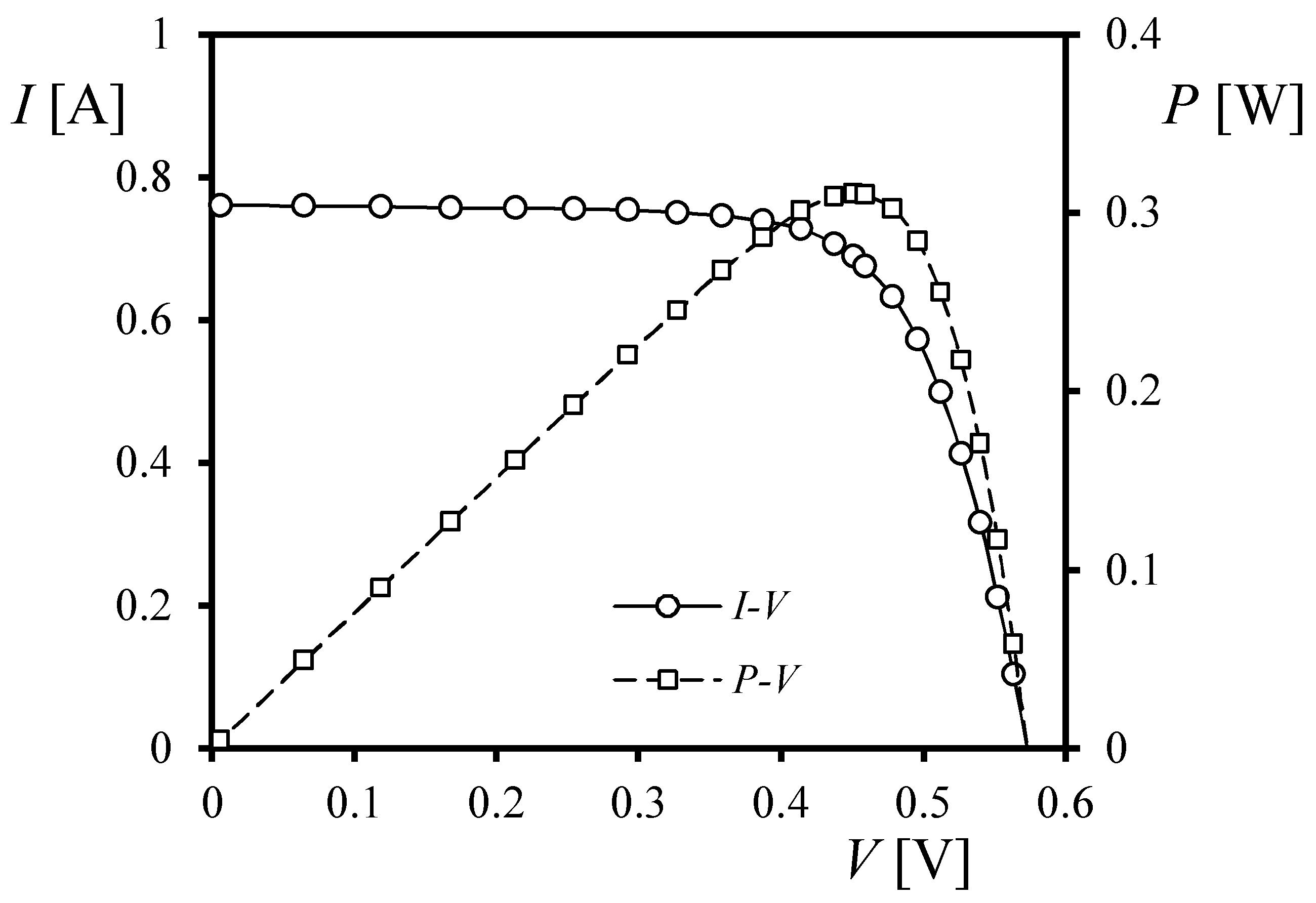
V curve of the solar cell/panel (see Figure 2), and defines the behavior of the photovoltaic device at a constant temperature and specific irradiance level. The equivalent circuit is comprised of a source that supplies the photocurrent, Ipv, a diode allowing ID1 current through it, and the series and shunt resistors Rs and Rsh. As indicated in the above mathematical expression, the diode is characterized by the saturation current, I0, the thermal voltage, VT, (defined as a function of the temperature, the charge of the electron, and the Boltzmann constant; see [1]), the ideality factor of the diode, a, and the number of series-connected cells in the photovoltaic device, n.
The above mathematical expression is, in fact, a simplified form of a more complex one involving two diodes connected in parallel rather than one:
I = I p v I 01 [ exp ( V + I R s n a 1 V T ) 1 ] I 02 [ exp ( V + I R s n a 2 V T ) 1 ] V + I R s R s h .
In the past, this 2-diode/2-resistor equation was suggested for solar cell modeling where all terms contain physical meaning [1]. Obviously, with the simplification to the 1-diode/2-resistor equation applied to solar panels comprised of several connected cells (or based on more evolved technologies such as multi-junction cells), the terms of Equation (1) have lost the direct modeling of the physical effects involved in the solar energy generation process. Nevertheless, that equation still retains physical meaning.
The parameter extraction process required to work with Equation (1) (i.e., to establish the correct values of parameters Ipv, I0, a, Rs, and Rsh) is usually a challenging process, not an immediate task. Many procedures and techniques have been developed to perform this extraction, see for example the works by Cotfas et al. [3], Tossa et al. [4], Ortiz-Conde et al. [5], Jena & Ramana [6], Chin et al. [7], Humada et al. [8], Ibrahim & Anani [9], and Abbassi et al. [10]. In addition, a number of calculations must be performed to work with Equation (1), as it is an implicit mathematical expression. In order to facilitate technical work with photovoltaic devices, explicit mathematical expressions have been proposed to obtain output current I directly, without using any algorithm, as a function of output voltage V. Obviously, these expressions have the following form:
I = f ( V , a 1 , a 2 , a 3 ... ) ,
where a1, a2, a3… are the parameters to be adjusted.
One might wonder why it is necessary to develop such immediate expressions when it is not difficult to accurately solve implicit equations by simply using commercial math software, such as MATLAB®. On the one hand, not all professionals in the solar energy sector can spare the resources (cost, training) to use such software. On the other, even skilled scientists/engineers need to find quick solutions in the predesign stages of projects involving photovoltaic devices. In these cases, the use of an appropriate explicit expression might be the best option. This need was detected while programming the power subsystem module at ESA’s Concurrent Design Facility (CDF) for the predesign of space missions at Instituto Universitario de Microgravedad “Ignacio Da Riva” (IDR/UPM), apart from other needs arising from academic and research work on space power systems at this institution [11,12,13]. Additionally, machine learning has become one of the most promising methodologies for performing performance prediction [14,15] and fault diagnosis [16,17,18,19] for solar energy systems. These methods normally include rather complicated 1-diode/2-resistor or 2-diode/2-resistor equivalent circuit parameter extraction techniques [20,21], such as genetic algorithms and particle swarm optimization [22,23,24]. The use of the explicit models included in this article might be also possible in machine learning.
It would be fair to cite some other lines of research, apart from explicit equations, developed to facilitate work with photovoltaic IV curves, or at least to reduce the difficulties of parameter extraction when working with the 1-diode/2-resistor model. First, the work of Toledo et al. [25,26,27,28] must be highlighted, as these researchers have developed different mathematical and iterative ways of performing such parameter extraction based on a reduced number of points from the IV curve. Second, some approximations to the parameters in Equation (1) have been proposed, based on experimental results. In this sense, a recent work by Gontean et al. [29] is worth mentioning, as these authors refer to a rather large number of quick approximations to the equivalent circuit parameters published in recent years.
The present study should be considered part of the research framework devoted to solar cell/panel behavior carried out since 2013 at the IDR/UPM Institute and the Aerospace Engineering School (Escuela Técnica Superior de Ingeniería Aeronáutica y del Espacio—ETSIAE) at the Polytechnic University of Madrid (Universidad Politécnica de Madrid—UPM). This research framework mainly focuses on the development of analytical models for studying solar cell/panel behavior for integration into more complex spacecraft mission simulators [1,30,31,32,33].
This paper includes a review and comparison of six explicit expressions (see Table 1) developed to describe the current–voltage behavior of solar cells/panels (i.e., the IV curve; see Figure 2). Apart from these six explicit equations for fitting the IV behavior curve of a photovoltaic device, we have found two more examples in the available literature. Xiao et al. proposed a six-order polynomial to fit the IV curve [34], which is, in fact, an interesting solution already used by other authors in their work [35,36]. However, due to the large number of parameters to be adjusted, this approximation was left out of the present study. In addition, Szabo and Gontean have very recently proposed the use of Bézier curves [37], but this approach was not considered here.
Several IV curves corresponding to different technologies were used to test the accuracy of these explicit expressions (see 
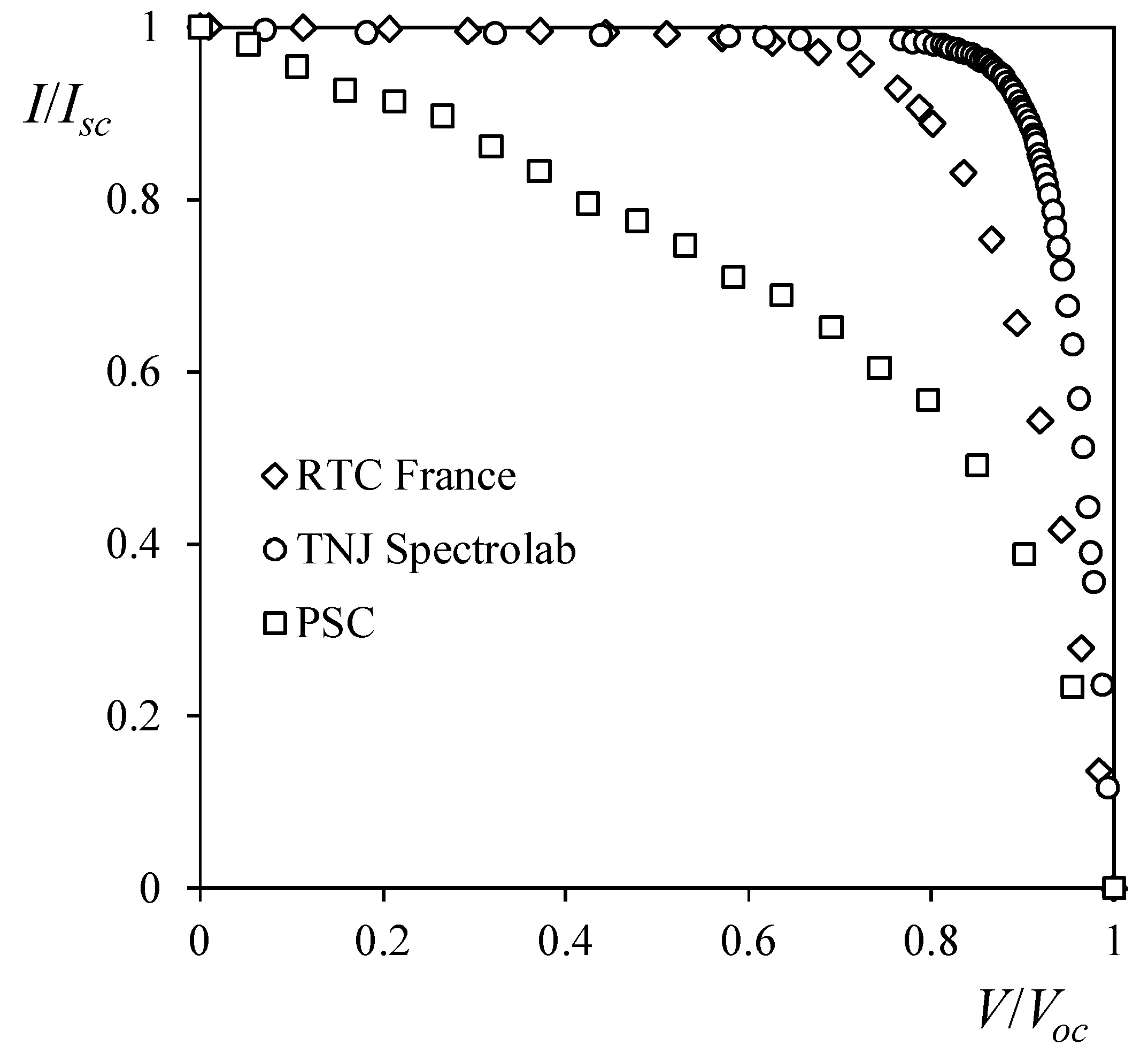
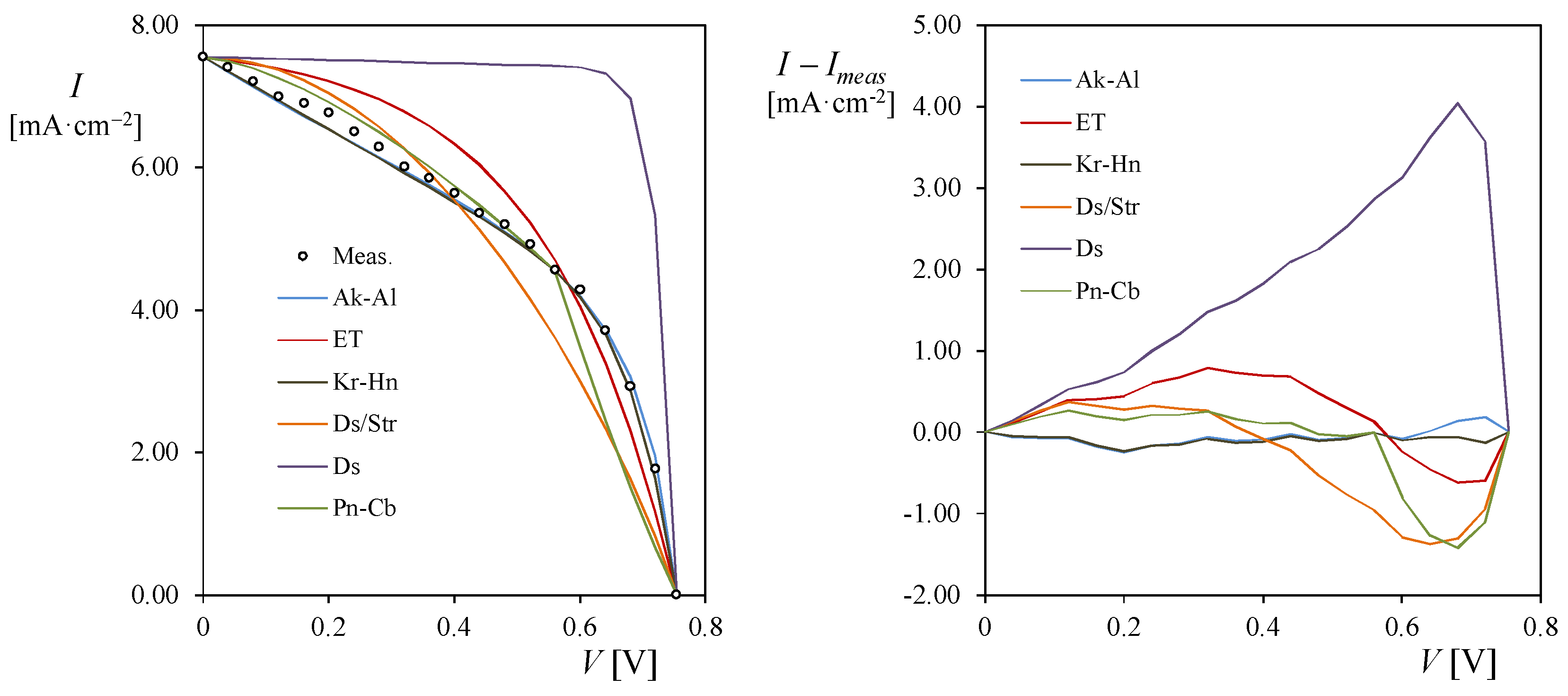
Table 2). It must also be said that plastic solar cells (PSCs) were one of the photovoltaic technologies used. PSCs have an IV curve slightly different from other, more mature, photovoltaic technologies (a much higher slope at the short-circuit point; see Figure 3). To the best of the authors’ knowledge, the first attempt to analyze these cells using explicit models is presented here, as an original contribution.
The explicit expressions were fitted using two methodologies:
  • adjusting the parameters of the expression using only the three characteristic points of the IV curve commonly supplied by the manufacturer (the short-circuit, open-circuit, and maximum power points; see Table 2), and
  • obtaining the best fit using a least squares method. This approach provides the most accurate expression for each model (i.e., equation) in relation to the data, but might not fulfill the characteristic conditions of the data (short-circuit, maximum power point, and open-circuit).
The explicit equations studied are described in Section 2, and Section 3 contains the results of the fittings and further discussion. Finally, the conclusions are summarized in Section 4.

2. Explicit Equations Studied

In this section, the six explicit equations analyzed are described, along with their analytical fitting to photovoltaic IV curves. As mentioned in the previous section, this fitting has been developed based on the three characteristic points of the IV curves: the short-circuit, open-circuit, and maximum power points. It should be also underlined that this information is generally supplied by the photovoltaic device manufacturer at Standard Test Conditions (STC), that is, at a specific level of irradiance and at a specific temperature of the solar cell/panel. In order to obtain the aforementioned characteristic points at different irradiance and temperature conditions, some authors, such as Bellini et al. [46], Siddiqui et al. [47], and Ibrahim & Anani [48], have suggested different procedures. These procedures were successfully used in a previous work related to spacecraft solar panel characterization with natural sun irradiance performed at the IDR/UPM Institute [49].

2.1. Akbaba & Alattawi (1995)

Akbaba & Alattawi suggested the following model for solar cell/panel behavior based on the following equation [38]:
I = V o c V A + B V 2 C V ,
where A, B, and C are the parameters to be adjusted.
In order to adjust parameters A, B, and C using the aforementioned characteristic points of the IV curve, the above equation can be rewritten in terms of non-dimensional variables (i = I/Isc and v = V/Voc):
i = 1 v 1 + a v 2 b v ,
bearing in mind that
A = V o c I s c ;   B = a I s c V o c ;   C = b I s c .
Please note that the number of parameters to be adjusted in Equation (4) has been reduced to two (a and b) in Equation (5), as mentioned in Section 1 (Table 1). If the equations for the maximum power point
( v , i ) | m p = ( α , β ) i v | m p = β α ,
are taken into account, it is possible to derive the following equations:
β = 1 α 1 + a α 2 b α ,
i v = β α = ( 1 + a α 2 b α ) + ( 1 α ) ( 2 a α b ) ( 1 + a α 2 b α ) 2 ,
where, according to Equations (7), α = Vmp/Voc and β = Imp/Isc. The following solutions can then be obtained:
a = β α α 2 β b = 2 β 1 α β .
Therefore, going back to Equations (6):
B = 1 V m p ( V o c I s c V m p 1 I m p ) C = V o c V m p ( 2 1 I s c 1 I m p ) .

2.2. El-Tayyan (2006)

El-Tayyan proposed a rather simple equation, relying on only two coefficients, C1 and C2:
I = I s c C 1 exp ( V o c C 2 ) [ exp ( V C 2 ) 1 ] ,
that can either be estimated or calculated based on the characteristic points of the IV curve [50]. The approximate solution proposed by El-Tayyan is as follows:
C 1 = I s c 1 exp ( V o c C 2 ) C 2 = V m p V s c ln ( 1 I m p I s c ) .
El-Tayyan’s equation is a rather simple mathematical expression. In fact, if we use the non-dimensional variables i = I/Isc and v = V/Voc, it can be reduced to a simpler form:
i = 1 exp ( a v ) 1 exp ( a ) 1 ,
dependent on only one parameter (a = Voc/C2), once the equation has proven to fulfill the short-circuit and open-circuit conditions, (i, v) = (1, 0) and (i, v) = (0, 1), respectively.
This implies that only one of the two conditions at the maximum power point (Equation (7)) can be fulfilled. The solution proposed by El-Tayyan fulfills the first condition; i.e., it fits the point (I, V) = (Imp, Vmp).
We found another solution that fulfills the second condition at the maximum power point (i.e., maximum power when V = Vmp). The following equation can be derived from the maximum power condition:
I V | m p = I m p V m p = C 1 C 2 exp ( V o c C 2 ) exp ( V m p C 2 ) .
Using the expression for C1 derived from the open-circuit condition (the first in Equation (13)), it is then possible to derive the following equation:
I m p V m p C 2 exp ( V m p C 2 ) = I s c 1 exp ( V o c C 2 ) exp ( V o c C 2 ) ,
where, assuming Voc/C2 >> 1:
C 2 = I s c V m p I m p exp ( V m p V o c C 2 ) ,
which can be solved using the negative branch of the Lambert function, W−1(z):
C 2 = V m p V o c W 1 [ ( 1 V o c V m p ) I m p I s c ] .
It is worth mentioning that a model very similar to El-Tayyan’s equation, which also considers changes in cell temperature, was proposed by Massi Pavan et al. [51,52]. Finally, it must also be said that after a thorough review of the available literature, we found evidence indicating that this model had been proposed before El-Tayyan’s work [53].

2.3. Karmalkar & Haneefa (2008)

Karmalkar & Haneefa proposed the following model [40,54]:
i = 1 ( 1 γ ) v γ v m ,
where i and v are the non-dimensional output current and output voltage (see Section 2.1), and γ and m are parameters to be calculated with the current and voltage levels at points v = 0.6 and i = 0.6.
Taking into account the characteristic points of the IV curve and the equations corresponding to the maximum power point (Equation (7)), the following equations can be derived for γ and m:
γ = 2 β 1 α m ( m 1 ) m = W 1 ( α 1 C ln α C ) ln α + 1 C + 1 ,
where α = Vmp/Voc, β = Imp/Isc, and the new parameter C is defined as
C = 1 β α 2 β 1 .
These are the exact solutions for γ and m, obtained from the maximum power conditions. Nevertheless, if we take into account that (1 − γ) << 1, the following approximated (and simpler) solutions are obtained:
γ = 1 + 1 β α m = ln ( 1 β ) ln α .
In addition, considering the approximation proposed by Deihimi et al. [55]:
i v | v = 1 1 i v | v = 0 ,
another simple equation can be obtained for γ, and the following solution can be derived:
γ = 2 m 1 m m = ln ( 1 β ) ln α .
Finally, it is fair to say that in 2015, Dash et al. [56] proposed a very similar equation to the one proposed by Karmalkar and Haneefa, but dependent on three parameters rather than two in the reduced form (non-dimensional variables).

2.4. Das; Saetre et al. (2011)

Das [41] and Saetre et al. [42] independently proposed the following equation:
I I s c = [ 1 ( V V o c ) f ] 1 g ,
where the model parameters f and g are estimated with output current measurements at V/Voc = 0.8 and V/Voc = 0.9.
Apart from this procedure, it is possible to derive a solution for parameters f and g. From the maximum power point conditions (7), the following equations are obtained:
β g = 1 α f ,
g β g = f α f ,
if we assume αf << 1, then
g ln ( β ) = ln ( 1 α f ) α f .
Therefore, the equations for the two parameters are finally defined as
f = 1 ln ( β ) g = α f ln ( β ) .

2.5. Das (2013)

Das proposed a simplified version of the previous model:
I I s c = 1 ( V V o c ) k 1 + h ( V V o c ) ,
where h and k are calculated with the slope of the IV curve at the short-circuit and open-circuit points [43]. Leaving this approach to extract the values of parameters h and k aside, it is possible to obtain an exact solution based on the maximum power point Equation (7). These equations, applied to the above expression, are
β = 1 α k 1 + h α ,
i v = β α = k α k 1 1 + h α + h ( 1 α k ) ( 1 + h α ) 2 .
From those equations, the following exact solution can be derived:
k = W 1 [ β ln ( α ) ] ln ( α ) h = 1 α ( 1 β 1 k 1 ) .
As in the case of the aforementioned equation proposed by Dash et al. [56], which was very similar to Karmalkar and Haneefa’s model, a modification to this implicit equation was suggested by Miceli et al. [57]. However, the reduced equation for this model depends on three parameters, making a solution based on the maximum power point conditions impossible.

2.6. Pindado & Cubas (2017)

Pindado & Cubas proposed a 2-expression equation to define the IV behavior of a photovoltaic device [32]:
I = { I s c [ 1 ( 1 I m p I s c ) ( V V m p ) I m p I s c I m p ] ;   V V m p I m p V m p V [ 1 ( V V m p V o c V m p ) η ] ;   V V m p .
Only one parameter, η, needs to be adjusted in this case. In addition, it must be highlighted that the maximum power point conditions (Equation (7)) are fulfilled by the above mathematical expressions (see [32]). The proposed equation for parameter η is:
η = I s c I m p ( I s c I s c I m p ) ( V o c V m p V o c ) .
However, it must be mentioned that the accuracy can be increased if data from one point between the maximum power point and the open-circuit point, V* and I*, is available. In this case
η = ln ( V m p I m p V * I * ) ln ( V m p I m p ) ln ( V * V m p ) ln ( V o c V m p ) .

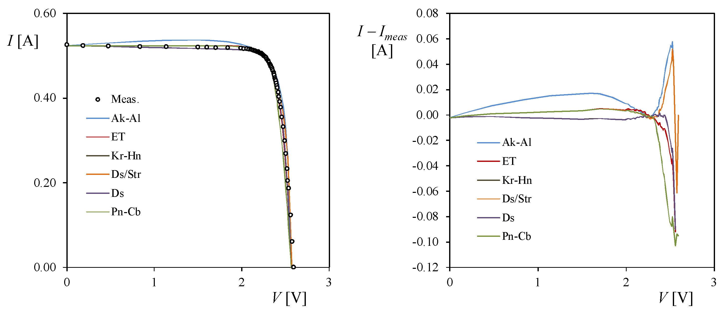
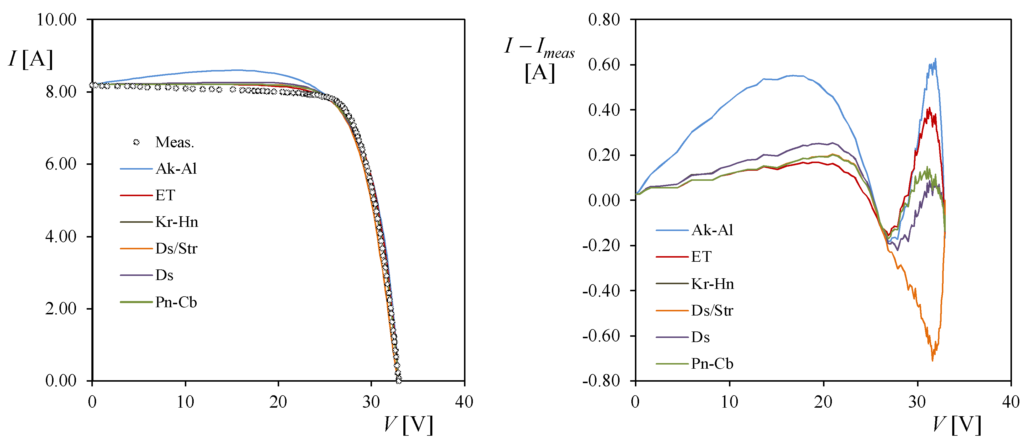
3. Results and Discussion

Figure 4, Figure 5, Figure 6, Figure 7, Figure 8, Figure 9, Figure 10 and 
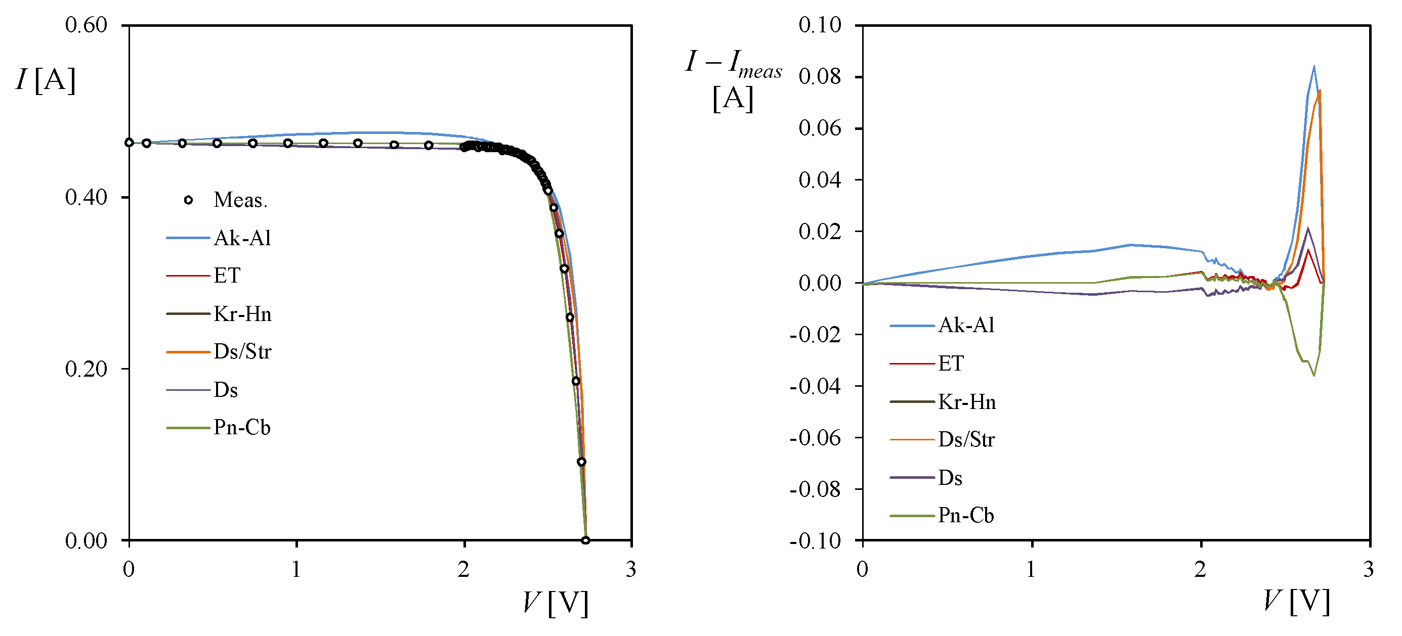
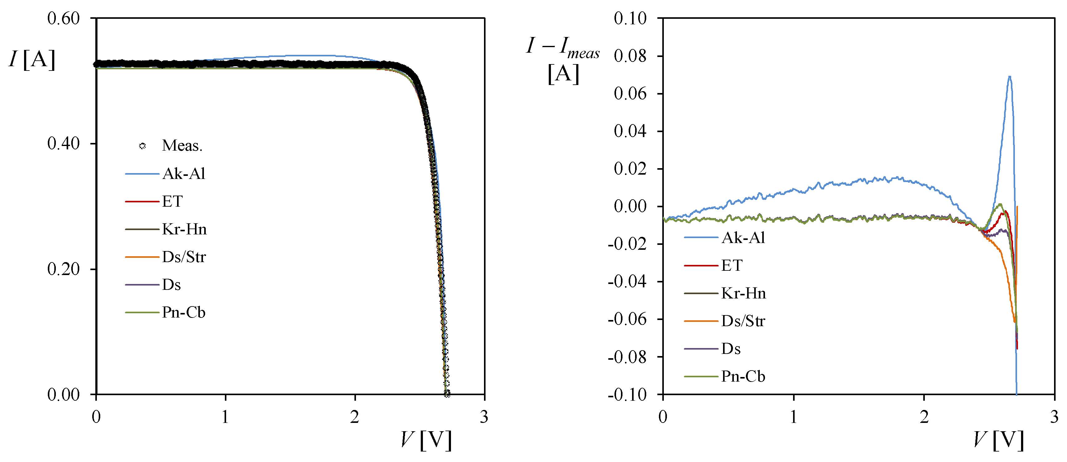
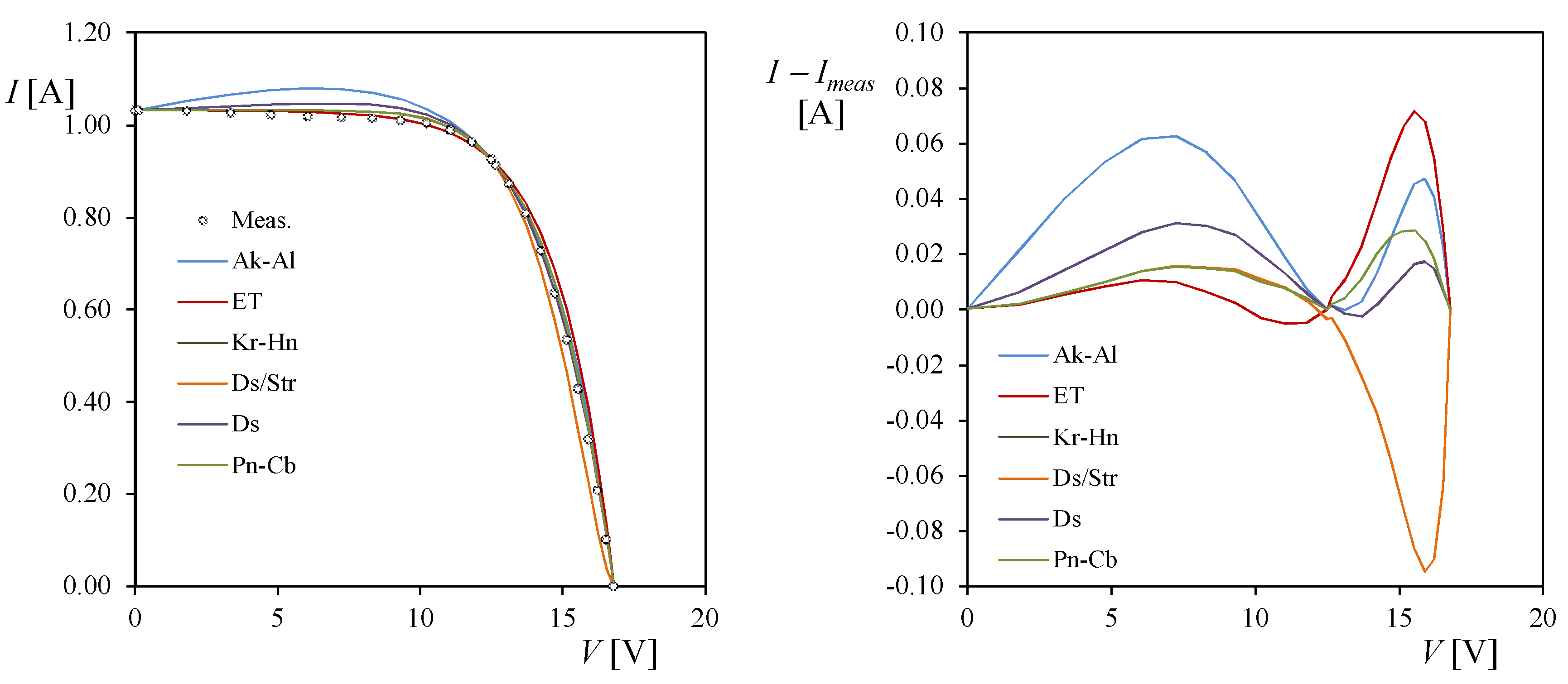
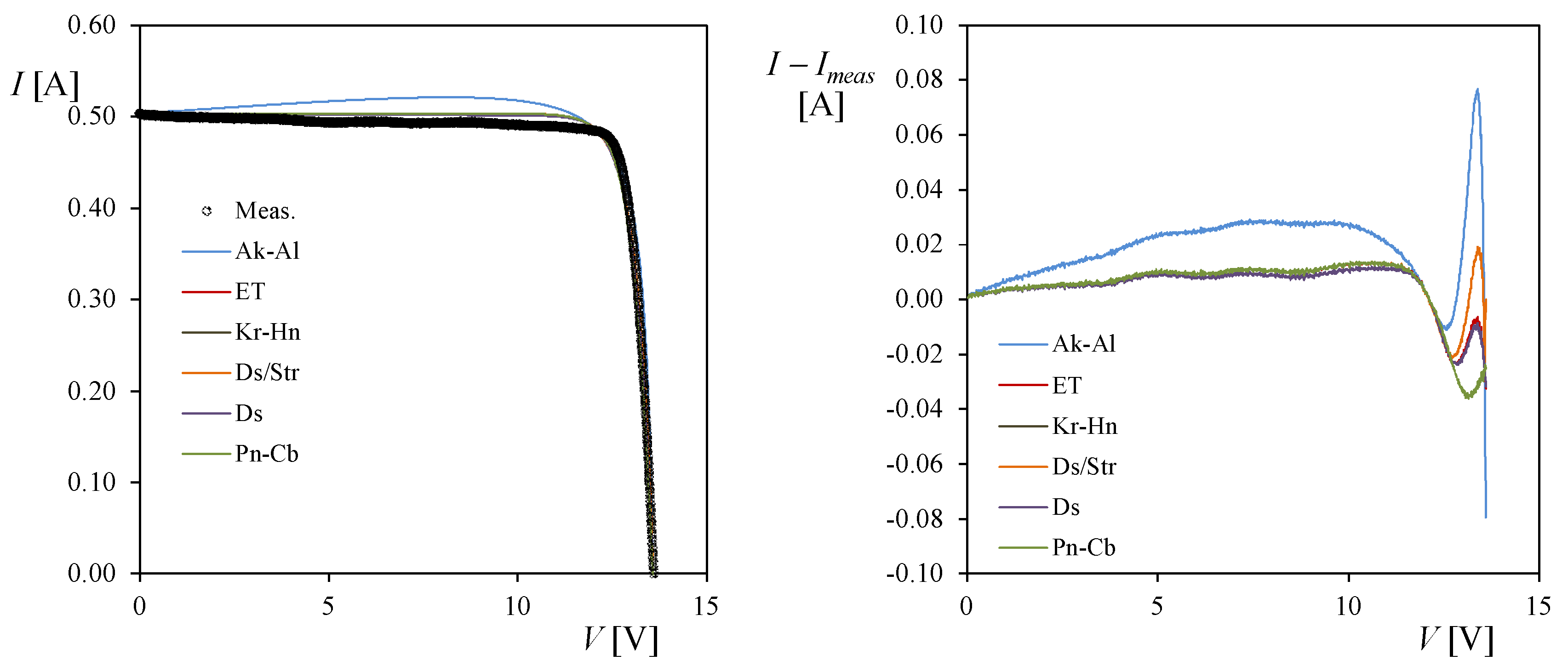
Figure 11 show the results of the explicit models studied (Akbaba & Alattawi: Ak-Al; El-Tayyan: ET; Karmalkar & Haneefa: Kr–Hn; Das/Saetra et al.: Da/Str; Das: Ds; Pindado & Cubas: Pn–Cb), fitted analytically to the measured IV curves using the characteristic point. Two graphs are included in these figures. The one on the left is a comparison of each model fitted to the experimental data. Since it is very difficult to appreciate the differences between the models on these graphs, a second one (on the left) has been included, in each case, to indicate the differences between the models and the original data; i.e., IImeas.
Table 3, Table 4, Table 5, Table 6, Table 7 and Table 8 include the coefficients of each model in relation to the measured data used in this benchmark. The coefficients corresponding to the best fit, obtained computationally, are also included in these tables.
The model represented in Figure 4, Figure 5, Figure 6, Figure 7, Figure 8, Figure 9, Figure 10 and Figure 11 is the one suggested by El-Tayyan (leaving aside suggested Equation (18)). Karmalkar & Haneefa’s equation model was solved with Equation (20). Both were the best options, as explained below.
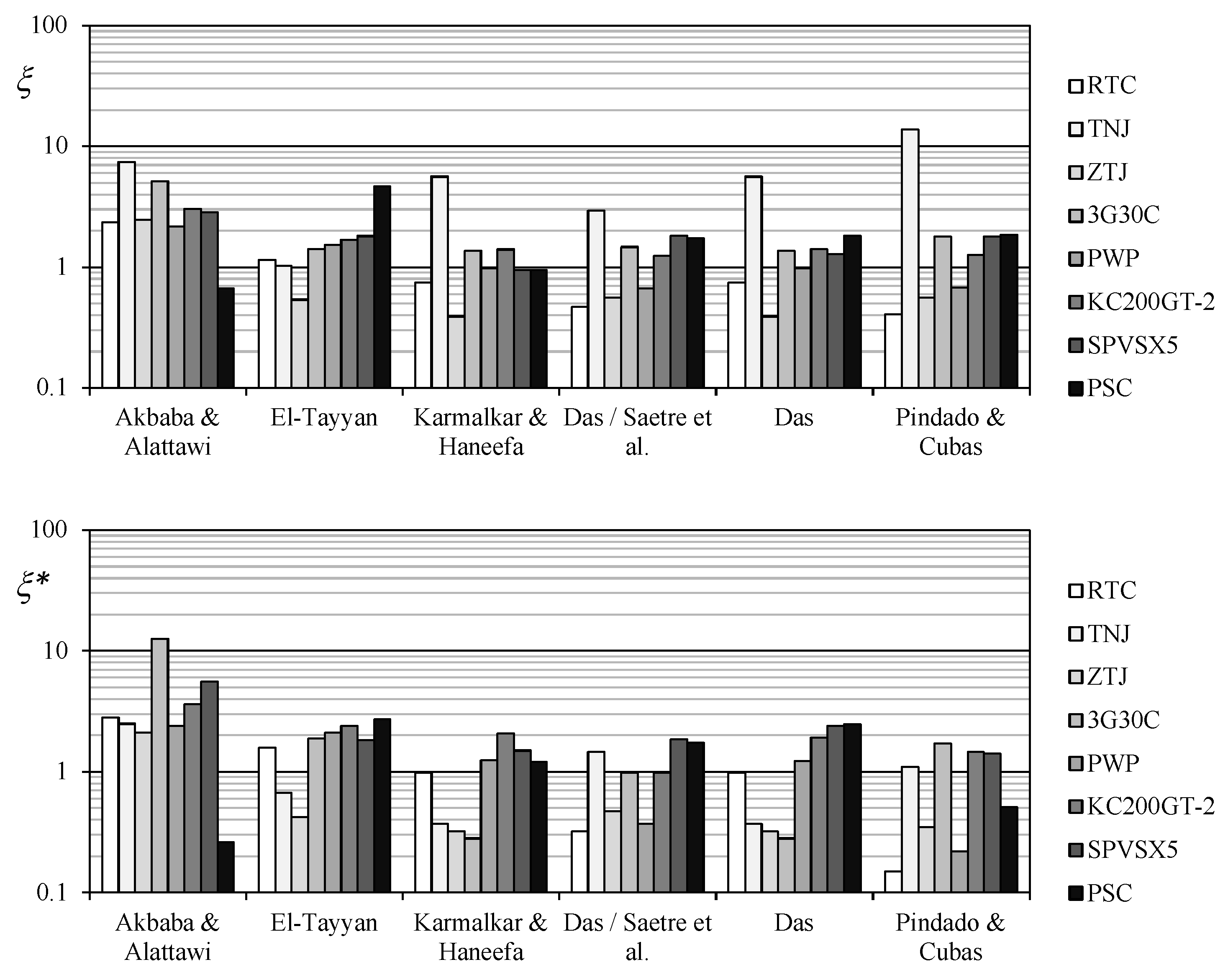
In the aforementioned figures, it is sometimes possible to distinguish the explicit model that provides the worst approximation to the data, but it is not possible to choose the best option with a proper criterion beyond a visual impression. For this reason, the results have been analyzed using the normalized RMSE:
ξ = 1 I s c 1 N j = 1 N ( I c a l c , j I j ) 2 .
Considering that the maximum power point is the optimum working point for a photovoltaic system, a second normalized RMSE value, ξ*, has been defined with the data within a ±5% bracket of the open-circuit voltage, Voc, around the maximum power point voltage, Vmp. These results are included in Table 3, Table 4, Table 5, Table 6, Table 7 and Table 8. Figure 12 includes the normalized RMSE values corresponding to the analytical fitting performed. In this figure, it seems that in the case of El-Tayyan’s model, the proposed methodology (Equation (18)) is less accurate when compared to the one proposed by this author (Equation (13)). Accordingly, if the fittings obtained with Karmalkar & Haneefa’s method are analyzed, it can be said that the first method proposed (Equation (20)) better fits the IV curves than the other two methodologies considered (Equations (22) and (23)). In addition, the normalized RMSE values corresponding to the best fittings of the explicit models are included in Table 3, Table 4, Table 5, Table 6, Table 7 and Table 8 and Figure 13. The results shown in this figure are obviously better than the ones in Figure 12. However, it must be considered that an explicit model is, indeed, a simplification when approaching a photovoltaic IV curve. Therefore, it might not make sense to use such simple equations and extract the parameters with a computational procedure. In any case, in order to establish a general comparison, all results from Figure 12 and Figure 13 have been averaged in Figure 14. Besides, the explicit models studied are ranked in Table 9, according to the data shown in Figure 14. Finally, the results corresponding to the 1-diode/2-resistor equivalent circuit model fitted to all the studied IV curves have been included in Table 10. Bearing in mind all of these results, it can be stated that:
  • Comparing the normalized RMSE values from the explicit models (Table 3, Table 4, Table 5, Table 6, Table 7 and Table 8) with the ones from the 1-diode/2-resistor equivalent circuit model (Table 10), it can be observed that the accuracy of the explicit models is similar to the accuracy of the 1-diode/2-resistor model.
  • The explicit model proposed by Karmalkar & Haneefa is the best one, taking into account all behavior (IV curves) of the different photovoltaic technologies used in this benchmark.
  • The model proposed by Das is also very accurate. However, when applied to plastic solar cell behavior, the results are very poor, in terms of accuracy.
  • The model proposed by Pindado & Cubas represents the best approach to the oldest silicon photovoltaic technology.
  • Surprisingly, Akbaba & Alattawi’s model is the one that best fits the behavior of the plastic solar cells, even though its results are the worst when applied to the other photovoltaic technologies studied.
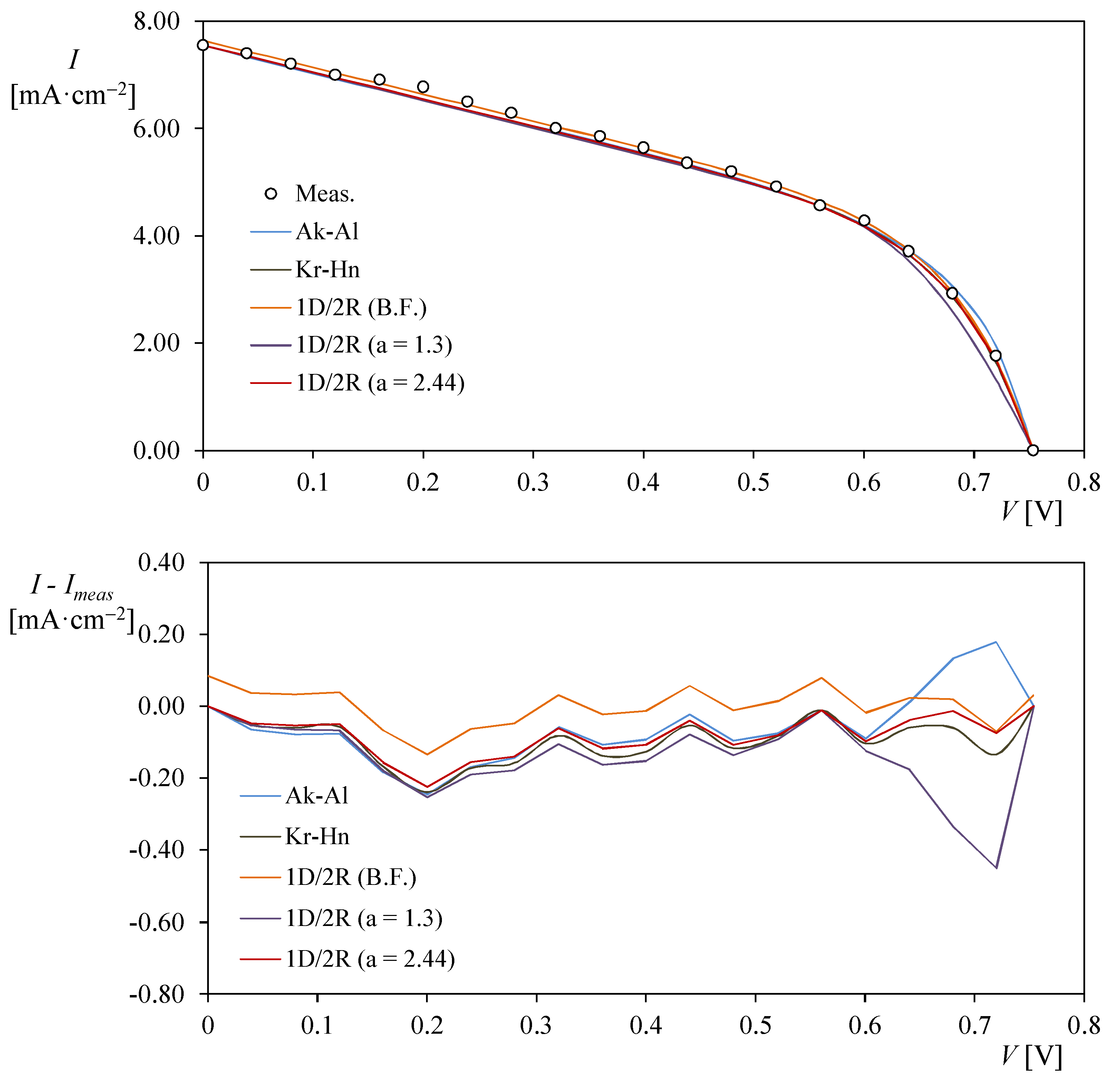
To continue with the results of the explicit models applied to plastic solar cells, Figure 15 shows the curves for the Akkbaba & Alattawi and Karmalkar & Haneefa models, along with three different fittings [1] of the 1-diode/2-resistor equivalent circuit model (Equation (1)): the best fit (performed computationally), analytical fitting with a = 1.3, and analytical fitting with a = 2.44 (close to the best value for this parameter). The figure shows that the explicit models (where ξ = 1.50% and 1.48%; see Table 3 and Table 5) are as accurate as the 1-diode/2-resistor equivalent circuit model (where ξ = 0.72%, 2.35% and 1.30%; see Table 10).

4. Conclusions

This study analyzes six different explicit mathematical expressions (i.e., explicit models) for describing the behavior of a solar cell/panel (by Akbaba & Alattawi; El-Tayyan; Karmalkar & Haneefa; Das/Saetre et al.; Das; and Pindado & Cubas). The models were fitted to the IV curves for eight different photovoltaic technologies.
The fittings were performed using the three characteristic points of the IV curves (short-circuit, maximum power, and open-circuit). A new definition of the parameters for each explicit model has been proposed. In order to compare across models, the best fitting of each model to the IV curves was also performed.
The major conclusions resulting from this study are:
  • The explicit models showed a performance as accurate as the 1-diode/2-resistor equivalent circuit model.
  • The explicit model that best fits in every case is the one proposed by Karmalkar & Haneefa. The second best in terms of accuracy is the one proposed by Das (However, its results were poor in the case of the plastic cell IV curve).
  • The accuracy of the explicit models studied depends on the photovoltaic technology. In the case of Si monocrystalline technology, the model proposed by Pindado & Cubas achieved the best results, whereas the simpler model by Akbaba & Alattawi fit extremely well to the plastic solar cell IV curve (with almost the same accuracy achieved by the 1-diode/2-resistor equivalent circuit model).

Author Contributions

Conceptualization, S.P.; Data curation, S.P.; Formal analysis, S.P., J.C., E.R.-M., F.B. and F.S.-P.; Methodology, S.P.; Validation, S.P. and J.C.; Writing—original draft, S.P.; Writing—review & editing, S.P., J.C., E.R.-M., F.B. and F.S.-P.

Acknowledgments

The authors are indebted to the students of the Master in Air Transport Systems and the Master in Space Systems of Universidad Politécnica de Madrid, for their hard work related to power systems which motivates and drives the authors’ research on the matter. The authors are indebted to the Reviewers for their comments, which helped us to improve this work. The authors are grateful to Tania Tate for her help in improving the style of the text.

Conflicts of Interest

The authors declare no conflict of interest.

References

  1. Cubas, J.; Pindado, S.; Victoria, M. On the analytical approach for modeling photovoltaic systems behavior. J. Power Sources 2014, 247, 467–474. [Google Scholar] [CrossRef]
  2. Easwarakhanthan, T.; Bottin, J.; Bouhouch, I.; Boutrit, C. Nonlinear Minimization Algorithm for Determining the Solar Cell Parameters with Microcomputers. Int. J. Sol. Energy 1986, 4, 1–12. [Google Scholar] [CrossRef]
  3. Cotfas, D.T.; Cotfas, P.A.; Kaplanis, S. Methods to determine the dc parameters of solar cells: A critical review. Renew. Sustain. Energy Rev. 2013, 28, 588–596. [Google Scholar] [CrossRef]
  4. Tossa, A.K.; Soro, Y.M.; Azoumah, Y.; Yamegueu, D. A new approach to estimate the performance and energy productivity of photovoltaic modules in real operating conditions. Sol. Energy 2014, 110, 543–560. [Google Scholar] [CrossRef]
  5. Ortiz-Conde, A.; García-Sánchez, F.J.; Muci, J.; Sucre-González, A. A Review of Diode and Solar Cell Equivalent Circuit Model Lumped Parameter Extraction. FACTA Univ. Ser. Electron. Energ. 2014, 27, 57–102. [Google Scholar] [CrossRef]
  6. Jena, D.; Ramana, V.V. Modeling of photovoltaic system for uniform and non-uniform irradiance: A critical review. Renew. Sustain. Energy Rev. 2015, 52, 400–417. [Google Scholar] [CrossRef]
  7. Chin, V.J.; Salam, Z.; Ishaque, K. Cell modelling and model parameters estimation techniques for photovoltaic simulator application: A review. Appl. Energy 2015, 154, 500–519. [Google Scholar] [CrossRef]
  8. Humada, A.M.; Hojabri, M.; Mekhilef, S.; Hamada, H.M. Solar cell parameters extraction based on single and double-diode models: A review. Renew. Sustain. Energy Rev. 2016, 56, 494–509. [Google Scholar] [CrossRef]
  9. Ibrahim, H.; Anani, N. Evaluation of Analytical Methods for Parameter Extraction of PV modules. Energy Procedia 2017, 134, 69–78. [Google Scholar] [CrossRef]
  10. Abbassi, R.; Abbassi, A.; Jemli, M.; Chebbi, S. Identification of unknown parameters of solar cell models: A comprehensive overview of available approaches. Renew. Sustain. Energy Rev. 2018, 90, 453–474. [Google Scholar] [CrossRef]
  11. Pindado, S.; Cubas, J.; Roibás-Millán, E.; Sorribes-Palmer, F. Project-based learning applied to spacecraft power systems: A long-term engineering and educational program at UPM University. CEAS Space J. 2018. [Google Scholar] [CrossRef]
  12. Pindado, S.; Sanz, A.; Sebastian, F.; Perez-grande, I.; Alonso, G.; Perez-Alvarez, J.; Sorribes-Palmer, F.; Cubas, J.; Garcia, A.; Roibas, E.; et al. Master in Space Systems, an Advanced Master’s Degree in Space Engineering. In Athens: ATINER’S Conference Paper Series, No. ENGEDU2016-1953; Athens Institute for Education and Research: Athens, Greece, 2016; pp. 1–16. [Google Scholar]
  13. Pindado Carrion, S.; Roibás-Millán, E.; Cubas Cano, J.; García, A.; Sanz Andres, A.P.; Franchini, S.; Pérez Grande, M.I.; Alonso, G.; Pérez-Álvarez, J.; Sorribes-Palmer, F.; et al. The UPMSat-2 Satellite: An academic project within aerospace engineering education. In Athens: ATINER’S Conference Paper Series, No. ENGEDU2017-2333; Athens Institute for Education and Research, ATINER: Athens, Greece, 2017; pp. 1–28. [Google Scholar]
  14. Li, H.; Liu, Z.; Liu, K.; Zhang, Z. Predictive Power of Machine Learning for Optimizing Solar Water Heater Performance: The Potential Application of High-Throughput Screening. Int. J. Photoenergy 2017, 2017, 4194251. [Google Scholar] [CrossRef]
  15. Liu, Z.; Li, H.; Liu, K.; Yu, H.; Cheng, K. Design of high-performance water-in-glass evacuated tube solar water heaters by a high-throughput screening based on machine learning: A combined modeling and experimental study. Sol. Energy 2017, 142, 61–67. [Google Scholar] [CrossRef]
  16. Chen, Z.; Wu, L.; Cheng, S.; Lin, P.; Wu, Y.; Lin, W. Intelligent fault diagnosis of photovoltaic arrays based on optimized kernel extreme learning machine and I–V characteristics. Appl. Energy 2017, 204, 912–931. [Google Scholar] [CrossRef]
  17. Madeti, S.R.; Singh, S.N. A comprehensive study on different types of faults and detection techniques for solar photovoltaic system. Sol. Energy 2017, 158, 161–185. [Google Scholar] [CrossRef]
  18. Wu, Y.; Chen, Z.; Wu, L.; Lin, P.; Cheng, S.; Lu, P. An Intelligent Fault Diagnosis Approach for PV Array Based on SA-RBF Kernel Extreme Learning Machine. Energy Procedia 2017, 105, 1070–1076. [Google Scholar] [CrossRef]
  19. Dhoke, A.; Sharma, R.; Saha, T.K. PV module degradation analysis and impact on settings of overcurrent protection devices. Sol. Energy 2018, 160, 360–367. [Google Scholar] [CrossRef]
  20. Abdin, Z.; Webb, C.J.; Gray, E.M.A. Simulation of large photovoltaic arrays. Sol. Energy 2018, 161, 163–179. [Google Scholar] [CrossRef]
  21. Triki-Lahiani, A.; Bennani-Ben Abdelghani, A.; Slama-Belkhodja, I. Fault detection and monitoring systems for photovoltaic installations: A review. Renew. Sustain. Energy Rev. 2018, 82, 2680–2692. [Google Scholar] [CrossRef]
  22. Pezzini, P.; Gomis-Bellmunt, O.; Sudri-Andreu, A. Optimization techniques to improve energy efficiency in power systems. Renew. Sustain. Energy Rev. 2011, 15, 2028–2041. [Google Scholar] [CrossRef]
  23. Precup, R.E.; Angelov, P.; Costa, B.S.J.; Sayed-Mouchaweh, M. An overview on fault diagnosis and nature-inspired optimal control of industrial process applications. Comput. Ind. 2015, 74, 75–94. [Google Scholar] [CrossRef]
  24. Zhao, Y.; Ball, R.; Mosesian, J.; de Palma, J.-F.; Lehman, B. Graph-Based Semi-supervised Learning for Fault Detection and Classification in Solar Photovoltaic Arrays. IEEE Trans. Power Electron. 2015, 30, 2848–2858. [Google Scholar] [CrossRef]
  25. Toledo, F.J.; Blanes, J.M.; Garrigós, A.; Martínez, J.A. Analytical resolution of the electrical four-parameters model of a photovoltaic module using small perturbation around the operating point. Renew. Energy 2012, 43, 83–89. [Google Scholar] [CrossRef]
  26. Toledo, F.J.; Blanes, J.M. Geometric properties of the single-diode photovoltaic model and a new very simple method for parameters extraction. Renew. Energy 2014, 72, 125–133. [Google Scholar] [CrossRef]
  27. Toledo, F.J.; Blanes, J.M. Analytical and quasi-explicit four arbitrary point method for extraction of solar cell single-diode model parameters. Renew. Energy 2016, 92, 346–356. [Google Scholar] [CrossRef]
  28. Toledo, F.J.; Blanes, J.M.M.; Galiano, V. Two-Step Linear Least-Squares Method for Photovoltaic Single-Diode Model Parameters Extraction. IEEE Trans. Ind. Electron. 2018, 65, 6301–6308. [Google Scholar] [CrossRef]
  29. Gontean, A.; Lica, S.; Bularka, S.; Szabo, R.; Lascu, D. A Novel High Accuracy PV Cell Model Including Self Heating and Parameter Variation. Energies 2017, 11, 36. [Google Scholar] [CrossRef]
  30. Cubas, J.; Pindado, S.; de Manuel, C. Explicit Expressions for Solar Panel Equivalent Circuit Parameters Based on Analytical Formulation and the Lambert W-Function. Energies 2014, 7, 4098–4115. [Google Scholar] [CrossRef]
  31. Cubas, J.; Pindado, S.; Manuel, C. De New Method for Analytical Photovoltaic Parameters Identification: Meeting Manufacturer’s Datasheet for Different Ambient Conditions. In International Congress on Energy Efficiency and Energy Related Materials (ENEFM2013); Oral, A.Y., Bahsi, Z.B., Ozer, M., Eds.; Springer International Publishing: Antalya, Turkey, 2014; Volume 155, pp. 161–169. [Google Scholar]
  32. Pindado, S.; Cubas, J. Simple mathematical approach to solar cell/panel behavior based on datasheet information. Renew. Energy 2017, 103, 729–738. [Google Scholar] [CrossRef]
  33. Cubas, J.; Pindado, S.; Sorribes-Palmer, F. Analytical calculation of photovoltaic systems maximum power point (MPP) based on the operation point. Appl. Sci. 2017, 7, 870. [Google Scholar] [CrossRef]
  34. Xiao, W.; Lind, M.G.J.; Dunford, W.G.; Capel, A. Real-Time Identification of Optimal Operating Points in Photovoltaic Power Systems. IEEE Trans. Ind. Electron. 2006, 53, 1017–1026. [Google Scholar] [CrossRef]
  35. Peng, L.; Sun, Y.; Meng, Z.; Wang, Y.; Xu, Y. A new method for determining the characteristics of solar cells. J. Power Sources 2013, 227, 131–136. [Google Scholar] [CrossRef]
  36. Andrei, H.; Ivanovici, T.; Predusca, G.; Diaconu, E.; Andrei, P.C. Curve fitting method for modeling and analysis of photovoltaic cells characteristics. In Proceedings of the 2012 IEEE International Conference on Automation Quality and Testing Robotics (AQTR), Cluj-Napoca, Romania, 24–27 May 2012; pp. 307–312. [Google Scholar]
  37. Szabo, R.; Gontean, A. Photovoltaic Cell and Module I–V Characteristic Approximation Using Bézier Curves. Preprints 2018. [Google Scholar] [CrossRef]
  38. Akbaba, M.; Alattawi, M.A.A. A new model for I-V characteristic of solar cell generators and its applications. Sol. Energy Mater. Sol. Cells 1995, 37, 123–132. [Google Scholar] [CrossRef]
  39. El Tayyan, A. An Empirical model for Generating the IV Characteristics for a Photovoltaic System. J. Al-Aqsa Unvi. 2006, 10, 214–221. [Google Scholar]
  40. Karmalkar, S.; Haneefa, S. A Physically Based Explicit J–V Model of a Solar Cell for Simple Design Calculations. IEEE Electron Device Lett. 2008, 29, 449–451. [Google Scholar] [CrossRef]
  41. Das, A.K. An explicit J–V model of a solar cell for simple fill factor calculation. Sol. Energy 2011, 85, 1906–1909. [Google Scholar] [CrossRef]
  42. Saetre, T.O.; Midtgard, O.M.; Yordanov, G.H. A new analytical solar cell I-V curve model. Renew. Energy 2011, 36, 2171–2176. [Google Scholar] [CrossRef]
  43. Das, A.K. An explicit J-V model of a solar cell using equivalent rational function form for simple estimation of maximum power point voltage. Sol. Energy 2013, 98, 400–403. [Google Scholar] [CrossRef]
  44. Jeranko, T.; Tributsch, H.; Sariciftci, N.S.; Hummelen, J.C. Patterns of efficiency and degradation of composite polymer solar cells. Sol. Energy Mater. Sol. Cells 2004, 83, 247–262. [Google Scholar] [CrossRef]
  45. Ortiz-Conde, A.; García Sánchez, F.J.; Muci, J. New method to extract the model parameters of solar cells from the explicit analytic solutions of their illuminated I–V characteristics. Sol. Energy Mater. Sol. Cells 2006, 90, 352–361. [Google Scholar] [CrossRef]
  46. Bellini, A.; Bifaretti, S.; Iacovone, V.; Cornaro, C. Simplified Model of a Photovoltaic Module. In Proceedings of the Applied Electronics, Pilsen, Czech Republic, 9–10 September 2009; pp. 47–51. [Google Scholar]
  47. Siddiqui, M.U.; Arif, A.F.M.; Bilton, A.M.; Dubowsky, S.; Elshafei, M. An improved electric circuit model for photovoltaic modules based on sensitivity analysis. Sol. Energy 2013, 90, 29–42. [Google Scholar] [CrossRef]
  48. Ibrahim, H.; Anani, N. Variations of PV module parameters with irradiance and temperature. Energy Procedia 2017, 134, 276–285. [Google Scholar] [CrossRef]
  49. Roibás-Millán, E.; Alonso-Moragón, A.; Jiménez-Mateos, A.; Pindado, S. Testing solar panels for small-size satellites: The UPMSAT-2 mission. Meas. Sci. Technol. 2017, 28, 115801. [Google Scholar] [CrossRef]
  50. El Tayyan, A.A. A simple method to extract the parameters of the single-diode model of a PV system. Turk. J. Phys. 2013, 37, 121–131. [Google Scholar]
  51. Massi Pavan, A.; Mellit, A.; Lughi, V. Explicit empirical model for general photovoltaic devices: Experimental validation at maximum power point. Sol. Energy 2014, 101, 105–116. [Google Scholar] [CrossRef]
  52. Massi Pavan, A.; Mellit, A.; De Pieri, D.; Lughi, V. A study on the mismatch effect due to the use of different photovoltaic modules classes in large-scale solar parks. Prog. Photovolt. Res. Appl. 2014, 22, 332–345. [Google Scholar] [CrossRef]
  53. Rauschenbach, H. Solar Cell Array Design Handbook; Jet Propulsion Laboratory, California Institute of Technology: Pasadena, CA, USA, 1976; Volume 1, p. 91103. [Google Scholar]
  54. Haneefa, S.; Karmalkar, S. An Analytical Method to Extract the Physical Parameters of a Solar Cell from Four Points on the Illuminated J–V Curve. IEEE Electron Device Lett. 2009, 30, 349–352. [Google Scholar]
  55. Deihimi, M.H.; Naghizadeh, R.A.; Meyabadi, A.F. Systematic derivation of parameters of one exponential model for photovoltaic modules using numerical information of data sheet. Renew. Energy 2016, 87, 676–685. [Google Scholar] [CrossRef]
  56. Dash, D.P.; Roshan, R.; Mahata, S.; Mallik, S.; Mahato, S.S.; Sarkar, S.K. A compact J-V model for solar cell to simplify parameter calculation. J. Renew. Sustain. Energy 2015, 7, 013127. [Google Scholar] [CrossRef]
  57. Miceli, R.; Orioli, A.; Di Gangi, A. A procedure to calculate the I-V characteristics of thin-film photovoltaic modules using an explicit rational form. Appl. Energy 2015, 155, 613–628. [Google Scholar] [CrossRef] [Green Version]
Figure 1. Solar cell/panel 1-diode/2-resistor equivalent circuit model [1].
Energies 11 01353 g001
Figure 2. Current–voltage (IV) and power–voltage (PV) curves of an RTC France Si solar cell [2].
Energies 11 01353 g002
Figure 3. Non-dimensional current–voltage curves for three solar cells based on different technologies (RTC France: silicon; TNJ Spectrolab: Ga–As triple junction; PSC: plastic solar cell. See Table 2).
Energies 11 01353 g003
Figure 4. Curves for the explicit models analyzed, fitted to the RTC France solar cell data using the analytical methods proposed; see Section 2 (left). The error in relation to the data is also included in the figure (right).
Energies 11 01353 g004
Figure 5. Curves for the explicit models analyzed, fitted to the TNJ Spectrolab solar cell data using the analytical methods proposed; see Section 2 (left). The error in relation to the data is also included in the figure (right).
Energies 11 01353 g005
Figure 6. Curves for the explicit models analyzed, fitted to the ZTJ Emcore solar cell data using the analytical methods proposed; see Section 2 (left). The error in relation to the data is also included in the figure (right).
Energies 11 01353 g006
Figure 7. Curves for the explicit models analyzed, fitted to the Azur Space 3G30C solar cell data using the analytical methods proposed; see Section 2 (left). The error in relation to the data is also included in the figure (right).
Energies 11 01353 g007
Figure 8. Curves for the explicit models analyzed, fitted to the Photowatt PWP 201 solar panel data using the analytical methods proposed; see Section 2 (left). The error in relation to the data is also included in the figure (right).
Energies 11 01353 g008
Figure 9. Curves for the explicit models analyzed, fitted to the Photowatt KC200GT-2 solar panel data using the analytical methods proposed; see Section 2 (left). The error in relation to the data is also included in the figure (right).
Energies 11 01353 g009
Figure 10. Curves for the explicit models analyzed, fitted to the Selex Galileo SPVSX5 solar cell module data using the analytical methods proposed; see Section 2 (left). The error in relation to the data is also included in the figure (right).
Energies 11 01353 g010
Figure 11. Curves for the explicit models analyzed, fitted to the plastic solar cell data using the analytical methods proposed; see Section 2 (left). The error in relation to the data is also included in the figure (right).
Energies 11 01353 g011
Figure 12. Comparison of the different explicit models studied, analytically fitted to the IV curves selected for the benchmark (Table 2). Normalized RMSE, ξ, (Equation (37)), and normalized RMSE within ±5% of Voc around the maximum power point, ξ*. See also Table 3, Table 4, Table 5, Table 6, Table 7 and Table 8. El-Tayyan (1) indicates Equation (13), whereas El-Tayyan (2) refers to Equation (18). Karmalkar & Haneefa (1) indicates Equation (20), Karmalkar & Haneefa (2) refers to Equation (22), and Karmalkar & Haneefa (3) indicates Equation (24).
Energies 11 01353 g012
Figure 13. Comparison of the different explicit models studied, computationally fitted (best fit) to the IV curves selected for the benchmark (Table 2). Normalized RMSE, ξ, (Equation (37)), and normalized RMSE within ±5% of Voc around the maximum power point, ξ*. See also Table 3, Table 4, Table 5, Table 6, Table 7 and Table 8.
Energies 11 01353 g013
Figure 14. General comparison of the explicit models studied for photovoltaic behavior (IV curves). Averaged values of data from Figure 13 and Figure 15.
Energies 11 01353 g014
Figure 15. Curves from the Akbaba & Alattawi and Karmalkar & Haneefa explicit models, fitted to plastic solar cell data using the analytical methods proposed (see Section 2), along with three fittings of the 1-diode/2-resistor equivalent circuit model defined by Equation (1) (above). The error in relation to the data is also included in the figure (below).
Energies 11 01353 g015
Table 1. Explicit equations for solar cell/panel behavior included in this study. The number of parameters in each equation proposed is included in the table. The number of parameters in the reduced equation refers to the number of parameters in the equation once it has been reduced to non-dimensional variables (i.e., non-dimensional output current and output voltage; see Section 2).
YearEquationNumber of Parameters
Original EquationReduced Equation
1995Akbaba & Alattawi [38]32
2006El-Tayyan [39]21
2008Karmalkar & Haneefa [40]22
2011Das [41], Saetre et al. [42]22
2013Das [43]22
2017Pindado & Cubas [32]11
Table 2. Solar cell/panel IV curves used by the authors to compare explicit expressions (see Table 1). The characteristic points (Isc, Imp, Vmp, and Voc) for these curves are included in the table.
Solar Cell/PanelTechnologyIsc [A]Imp [A]Vmp [V]Voc [V]
RTC France 1Si0.76050.68940.45070.5727
TNJ Spectrolab 2GaInP2/GaAs/Ge0.52390.49602.2702.565
ZTJ Emcore 2InGaP/InGaAs/Ge0.46280.43892.4102.726
Azur Space 3G30C 3GaInP/GaAs/Ge0.52020.50442.4112.70
Photowatt PWP 201 1Si1.0320.925512.49316.778
Kyocera KC200GT-2 2Si polycrystalline8.2107.61026.3032.90
Selex Galileo SPVS X5 4GaInP/GaAs/Ge0.503440.4847612.09913.575
Plastic Solar Cell 5MDMO-PPV/PCBM [44]7.5514 64.5379 60.561760.75365
1 From [2]. 2 Graphically extracted from the manufacturer’s datasheet. 3 Supplied by Azur Space. 4 Measured at CIEMAT (Spain). 5 Graphically extracted from [45]. 6 Units: mA·cm−2.
Table 3. Parameters from Akbaba and Alattawi’s explicit model (Equation (4)), fitted to the IV curves for the photovoltaic devices studied (see Table 1). The fittings were performed numerically (Best fit), and using the proposed method (Equations (6), (10), and (11)). The normalized RMSE values of the fittings, ξ, and ξ*, are included in the table.
Proposed Method
Solar Cell/PanelABCξ [%]ξ* [%]
RTC France0.75310.48881.49853.890.35
TNJ Spectrolab4.89600.06202.035518.791.14
ZTJ Emcore5.89020.06872.31104.020.92
Azur Space 3G30C5.19030.07062.08533.431.67
Photowatt PWP 20116.25780.01771.15163.310.36
Kyocera KC200GT-24.00730.00080.14044.381.60
Selex Galileo SPVS X526.96450.01372.14284.961.77
Plastic Solar Cell0.0998−0.07600.05971.500.71
Best Fit
Solar Cell/PanelABCξ[%]ξ*[%]
RTC France0.77690.65311.61272.352.82
TNJ Spectrolab5.38560.25202.68137.412.49
ZTJ Emcore6.11900.14132.57322.462.10
Azur Space 3G30C5.2420.0692.07335.1312.6
Photowatt PWP 20116.79120.01941.20472.172.39
Kyocera KC200GT-24.24600.00110.15783.033.63
Selex Galileo SPVS X527.82390.01442.20762.845.57
Plastic Solar Cell0.09919−0.06120.067560.670.26
Table 4. Parameters from El-Tayyan’s explicit model Equation (12), fitted to the IV curves for the photovoltaic devices studied (see Table 1). The fittings were performed numerically (best fit) with El-Tayyan’s formulae (Equation (13)), and using the proposed method (Equations (16) and (18)). The normalized RMSE values of the fittings, ξ, and ξ*, are included in the table.
El-Tayyan
Solar Cell/PanelC1C2ξ [%]ξ* [%]
RTC France0.7605110.0514792.200.46
TNJ Spectrolab0.52390.1005915.730.87
ZTJ Emcore0.46280.1066340.570.32
Azur Space 3G30C0.52020.0827081.832.10
Photowatt PWP 2011.0321421.8867433.030.61
Kyocera KC200GT-28.2100182.5227642.301.34
Selex Galileo SPVS X50.503440.4480862.092.42
Plastic Solar Cell7.7618230.2088896.513.06
Proposed Method
Solar Cell/PanelC1C2ξ[%]ξ*[%]
RTC France0.7605260.0557621.351.74
TNJ Spectrolab0.52390.0898165.931.51
ZTJ Emcore0.46280.0966591.591.43
Azur Space 3G30C0.52020.0858611.962.62
Photowatt PWP 2011.0332142.4868224.067.23
Kyocera KC200GT-28.2100932.8889532.384.32
Selex Galileo SPVS X50.503440.4404922.022.25
Plastic Solar Cell7.5518220.0767719.9930.82
Best Fit
Solar Cell/PanelC1C2ξ[%]ξ*[%]
RTC France0.7792780.0547291.141.57
TNJ Spectrolab0.4264840.110641.030.67
ZTJ Emcore0.4654120.1074370.540.42
Azur Space 3G30C0.4772180.0837891.421.88
Photowatt PWP 2011.0642692.0422691.542.10
Kyocera KC200GT-28.3773732.6304881.682.38
Selex Galileo SPVS X50.4890230.4221921.811.82
Plastic Solar Cell7.26690.30614.652.71
Table 5. Parameters from Karmalkar and Haneefa’s explicit model Equation (19)), fitted to the IV curves for the photovoltaic devices studied (see Table 1). The fittings were performed numerically (best fit), and using the methodologies proposed (proposed method 1: Equation (20); (proposed method 2: Equation (22); and (proposed method 3: Equation (24)). The normalized RMSE values of the fittings, ξ, and ξ*, are included in the table.
Proposed Method 1
Solar Cell/Panelγmξ [%]ξ* [%]
RTC France0.99557610.032581.160.10
TNJ Spectrolab0.97779827.587555.670.21
ZTJ Emcore0.98023927.241650.970.37
Azur Space 3G30C1.00170530.447691.902.30
Photowatt PWP 2011.0396246.9803681.500.30
Kyocera KC200GT-21.01437411.095931.701.74
Selex Galileo SPVS X50.9944129.820971.952.35
Plastic Solar Cell0.49224510.800941.480.79
Proposed Method 2
Solar Cell/Panelγmξ [%]ξ* [%]
RTC France0.8812029.8926695.208.11
TNJ Spectrolab0.93982524.003167.615.62
ZTJ Emcore0.94158624.052034.094.92
Azur Space 3G30C0.96598630.864753.425.09
Photowatt PWP 2010.8614067.7012855.338.67
Kyocera KC200GT-20.90857911.684394.547.96
Selex Galileo SPVS X50.95836928.616932.554.91
Plastic Solar Cell0.4646143.12612711.9517.67
Proposed Method 3
Solar Cell/Panelγmξ [%]ξ* [%]
RTC France0.8875489.8926694.907.67
TNJ Spectrolab0.95652824.003166.904.30
ZTJ Emcore0.9566224.052033.013.69
Azur Space 3G30C0.96651630.864753.395.05
Photowatt PWP 2010.8507757.7012855.799.34
Kyocera KC200GT-20.90640611.684394.658.11
Selex Galileo SPVS X50.9637928.616932.414.53
Plastic Solar Cell0.5296613.12612710.5415.33
Best Fit
Solar Cell/Panelγmξ [%]ξ* [%]
RTC France0.998649.5275420.750.99
TNJ Spectrolab0.99087826.229125.620.37
ZTJ Emcore0.9926424.947960.390.32
Azur Space 3G30C1.0215632.029441.370.28
Photowatt PWP 2010.9993527.2815320.991.25
Kyocera KC200GT-20.9872511.873271.402.08
Selex Galileo SPVS X50.96668235.305490.941.49
Plastic Solar Cell0.521910.26710.951.21
Table 6. Parameters from Das/Saetre’s explicit model (Equation (25)), fitted to the IV curves for the photovoltaic devices studied (see Table 1). The fittings were performed numerically (best fit), and using the proposed method (Equation (29)). The normalized RMSE values of the fittings, ξ, and ξ*, are included in the table.
Proposed Method
Solar Cell/Panelfgξ [%]ξ* [%]
RTC France10.188020.8874250.670.58
TNJ Spectrolab18.273221.9597942.710.44
ZTJ Emcore18.85961.8466213.220.42
Azur Space 3G30C32.421480.825622.322.56
Photowatt PWP 2019.1810660.612414.040.60
Kyocera KC200GT-213.177010.6894184.332.14
Selex Galileo SPVS X526.44761.2596831.972.34
Plastic Solar Cell1.963571.1027048.7311.55
Best Fit
Solar Cell/Panelfgξ [%]ξ* [%]
RTC France10.146920.9180140.470.32
TNJ Spectrolab15.646592.2247132.961.46
ZTJ Emcore24.214971.005820.560.47
Azur Space 3G30C35.385470.9436881.470.98
Photowatt PWP 2017.8680170.9044680.670.37
Kyocera KC200GT-212.569280.9040711.250.99
Selex Galileo SPVS X532.682950.9989381.821.85
Plastic Solar Cell1.08082.42961.741.74
Table 7. Parameters from Das’s explicit model (Equation (30)), fitted to the IV curves for the photovoltaic devices studied (see Table 1). The fittings were performed numerically (best fit), and using the proposed method (Equation (33)). The normalized RMSE values of the fittings, ξ, and ξ*, are included in the table.
Proposed Method
Solar Cell/Panelkhξ [%]ξ* [%]
RTC France10.036770.0044471.150.10
TNJ Spectrolab27.604770.0226275.670.21
ZTJ Emcore27.257430.0200970.970.37
Azur Space 3G30C30.44602−0.00171.902.30
Photowatt PWP 2016.93745−0.039041.500.30
Kyocera KC200GT-211.08133−0.014261.701.74
Selex Galileo SPVS X529.82610.0056181.952.35
Plastic Solar Cell1.963571.1027048.7311.55
Best Fit
Solar Cell/Panelkhξ [%]ξ* [%]
RTC France9.5296590.0014060.750.99
TNJ Spectrolab26.238450.0092055.620.37
ZTJ Emcore24.954630.0074040.390.32
Azur Space 3G30C32.00393−0.021191.370.28
Photowatt PWP 2017.27740.00010.991.23
Kyocera KC200GT-211.67170.00511.421.91
Selex Galileo SPVS X532.15670.03041.282.41
Plastic Solar Cell8.31390.6041.822.48
Table 8. Parameters from Pindado and Cubas’s explicit model (Equation (34)), fitted to the I-V curves for the photovoltaic devices studied (see Table 1). The fittings were performed numerically (Best fit), and using the proposed method (Equation (35)). The normalized RMSE values of the fittings, ξ, and ξ*, are included in the table.
Proposed Method
Solar Cell/Panelηξ [%]ξ* [%]
RTC France2.51360.410.14
TNJ Spectrolab2.281114.572.48
ZTJ Emcore2.36691.890.90
Azur Space 3G30C3.63451.811.74
Photowatt PWP 2012.75961.400.30
Kyocera KC200GT-22.96141.361.41
Selex Galileo SPVS X53.04332.672.31
Plastic Solar Cell1.06177.190.51
Best Fit
Solar Cell/Panelηξ [%]ξ* [%]
RTC France2.5200.410.15
TNJ Spectrolab3.56013.731.10
ZTJ Emcore2.9000.560.35
Azur Space 3G30C3.7201.791.72
Photowatt PWP 2012.4800.680.22
Kyocera KC200GT-22.8501.261.46
Selex Galileo SPVS X53.8501.801.41
Plastic Solar Cell3.3001.850.51
Table 9. Ranking of the explicit models studied, based on accuracy results (see Figure 15), by photovoltaic technology (see Table 1 and Table 2).
ModelRTC FranceTNJ SpectrolabZTJ EmcoreAz-Sp 3G30CPhotowatt PWP 201Kyocera KC200GT-2Slx-Ga SPVS X5PSC
Karmalkar & Haneefa43213312
Das33212236
Pindado & Cubas16421153
El-Tayyan52135444
Das/Saetre et al.21544525
Akbaba & Alattawi65656661
Table 10. Parameters from the 1-diode/2-resistor equivalent circuit model fitted to all studied curves. The values related to the plastic solar cell (PSC) IV curve are best fit (calculated as the correspondent to the other technologies, see also [32]); analytical fitting where a = 1.30; and analytical fitting where a = 2.44). The normalized RMSE values of the fittings, ξ, and ξ*, are included in the table.
ModelaIpv [A]I0 [A]Rs [Ω]Rsh [Ω]ξ [%]ξ* [%]
RTC France1.487.61 × 1013.20 × 1073.62 × 1025.20 × 1010.090.07
TNJ Spectrolab1.015.24 × 1013.49 × 10155.51 × 1022.08 × 1025.430.32
ZTJ Emcore1.074.63 × 1012.78 × 10157.41 × 1022.73 × 1020.700.32
Azur Space 3G30C0.95.20 × 1019.55 × 10187.95 × 1022.62 × 1032.452.62
Photowatt PWP 2011.251.031.28 × 1061.563.55 × 1031.190.27
Kyocera KC200GT-218.234.03 × 10103.36 × 1011.59 × 1023.842.04
Selex Galileo SPVS X51.155.03 × 1011.48 × 10142.40 × 1029.69 × 1031.972.30
PSC 12.44737.70652.42·1051.84481990.720.75
PSC (a = 1.3) 11.308.23711.14·10916.1331782.350.87
PSC (a = 2.44) 12.447.59673.11·1050.482121991.300.76
1 PSC current units: mA·cm−2.

