Cross Test Comparison in Transformer Windings Frequency Response Analysis

Abstract

Frequency Response Analysis (FRA) is an important tool used for diagnostic measurements of power transformers. Standard test configuration applied in the industry is the end-to-end open test setup; however, an interwinding capacitive configuration is also used. This paper presents a method—Cross Test Comparison (CTC)—for simultaneous analysis of results coming from both the mentioned test setups. Such an approach could offer a more sensitive tool for detecting some faults; moreover, it takes into consideration the influence of both voltage sides of a transformer in a one test result. The authors have used several indices to quantitatively assess the test results and proposed new approach to data interpretation. CTC method was tested using data from measurements performed in three cases: a unit tested in laboratory with introduced controlled deformations; transformers measured under industrial conditions; and a transformer with FRA changes resulting from tap-changer operations. The results showed that CTC method is more effective at detecting faults on the basis of FRA measurements.

1. Introduction

Transformers are very important apparatus in power systems, as they directly determine energy transmission reliability. During operation, the active part of a transformer is exposed to mechanical stresses, which may result in local deformations of windings or in electric faults. Frequency Response Analysis (FRA) is an important tool used in the diagnosis of power transformers. This method compares low voltage sinusoidal signal, of variable frequency, applied at one end of the winding and registered at the other end of the winding or the opposite voltage side. Such comparison in the wide frequency range allows for detecting changes in the electrical parameters of the transformer’s active part. FRA is used to detect mechanical faults in the windings, as well as some problems in the core. In a transformer, such problems could arise due to forces related to short-circuit currents, especially in units with aged solid insulation, which have lost its elasticity. Improper transportation of a unit could also be another source of internal mechanical faults. A transformer with deformed winding could still be operated under nominal conditions, however during subsequent network event, it may lead to transformer internal short circuit with a risk of transformer fire and all costs related to power outage and unit’s repairs or replacement. Thus, early and reliable diagnostics is a key factor in modern management of power systems assets [1,2,3,4,5].

At the current stage of FRA method development, it is possible to perform repetitive measurements. In 2012, an IEC (International Electrotechnical Commission) standard on a measuring technology [6] was published, and most available commercial devices fulfill its requirements. However there still exist problems with interpretation of test results. Various approaches and automated tools are currently in use, but still it is problematic to assess cases indicating changes between compared curves. Due to varying designs of transformers and their power ratings, it is difficult to judge what kind and scale of difference between compared curves (amplitude damping and/or frequency shift) could be classified as obvious deformation.

Typically, in industrial measurements, results are recorded in one test configuration: end-to-end open (E2E). In such case, only the winding of measured voltage side is taken under consideration, with some capacitive influence of other windings. There are also other test setups, e.g., interwinding capacitive (IntCap), which can provide valuable information on windings geometry, but usually are not used in practice and even if tests are taken in two setup configurations their results are analyzed separately [7,8,9,10].

This paper presents a method for simultaneous analysis of results from both the mentioned test setups. Such an approach turns out to be a more effective tool for detecting some faults, and, in addition, it binds the influence of both voltage sides of a transformer in a one test result. It is difficult to review the transformer as three separate columns, because one side is usually delta connected, so there is direct influence of other columns on the tested one, even under such low voltage signal conditions as used in FRA method. Through capacitive and inductive couplings, there is also relation between the high and low voltage sides. Therefore the analysis of results obtained from both end-to-end measurement as well as interwinding capacitive measurement gives results coming directly from two windings (high and low voltage side) geometry.

Changes in the frequency response (FR) for given deformation in the windings are visible in various frequency ranges for both mentioned test setups; in E2E in narrower range, while for IntCap, it is wider frequency spectrum. The simultaneous analysis of such results shows bigger differences than each test setup analyzed separately, which is expected, but allows for assessment of all changes with a single formula.

2. FRA Measurements and Results Interpretation

FRA test result assessment is performed usually by a professional technician, however, currently a number of automatic tools are being developed for this purpose, e.g., algorithms based on various mathematical formulas. However, interpretation of measured data remains an issue, as these algorithms do not have clear assessment criteria. In addition, FRA is a strictly comparative method, but still in some cases reference data is not accessible, so measurement results must be compared with results from sister or twin units, sometimes with results of other units of the same type. Yet another approach, very popular in the industry, is comparison between phases of the tested unit, however, in this case too, there is a big risk of misinterpretation. FRA test results are typically presented in the form of Bode plots, with damping in (dB) and phase angle shift presented separately in a logarithmic frequency scale. Sometimes, a linear frequency scale is used for Bode graphs or other forms of presentation, e.g., polar plots. During assessment, the FR range is usually divided into three main subranges, sometimes including additional sub-bands. These ranges are as follows: low, medium and high frequencies. Their borders depend on the construction of the transformer, mainly on its geometrical size, usually related to its power rating. Therefore, it is not possible to perform analysis in predefined frequency ranges. The bigger transformer, the higher the values of inner capacitances, thus the frequency response is shifted into lower frequencies [6]. In the case there are differences in the FRA results for different phases or transformers compared, it would not be apparent whether they have their origin in the deformation in the active part or they arise from natural differences between compared units. In the best case, when compared curves that show differences come from the same phase of a transformer and were recorded in some time interval, it would be clear that there are some changes in the active part or winding connection setup, yet it is not possible usually to assess the scale and location of the deformation [2,11]. Therefore, for these reasons, there is a need to develop new approaches of data assessment.

FR can be measured in various test configurations, however, according to the standard [6], the main configuration is end-to-end open test setup, where the signal is applied to the beginning of the winding and measured at its end, with remaining windings left open. Another test setup configuration is based on capacitive couplings between windings of the same phase, without galvanic connection between them—it is the interwinding capacitive test setup. The signal is applied to the beginning of one winding (usually HV side) and measured at the beginning of the other winding (LV). The other ends of both windings are left open. These two test setups have different responses, especially at low frequency range, where there is a significant influence of transformer’s bulk capacitances on FR (creating together with core’s inductance the first parallel resonance). However, when results coming from the same test setup are compared e.g., with results from other phases or from other units, they have similar shape. In other words what was the test setup can be easily found on the basis of curve shape. Figure 1 presents schematic connection of both the mentioned test setups (Figure 1a,c) and exemplary responses (Figure 1d,e). Additionally the connection setup for delta connected windings is presented in Figure 1b.

FRA graphs can be divided into three main frequency ranges: low frequency (LF) influenced mostly by bulk capacitances to the ground and the windings’ main magnetizing inductance, which ends in the inflection point after the first parallel resonance; medium frequency (MF) influenced by interactions between local capacitances and inductances, used for detection of deformations—it ends approx. in the half of range from the LF range end to the end of measuring frequency (2 MHz) in the logarithmic scale; and remaining high frequency range (HF)—strongly influenced by a test setup and other factors that are usually omitted in the analysis [2,6,8,10,11]. In the lowest frequency range winding inductances are dominant resulting in decreasing slope. When the first resonance is reached a dominant influence of winding capacitances appears. In the MF range the influence of the magnetic circuit disappears and the shape of FRA curve is determined by interaction of magnetic couplings and local capacitances. The HF range is influenced by many additional parameters, including wave phenomena and therefore is difficult for direct assessment. Of course it is not possible to distinguish direct parameters that create given resonance, as all winding geometry—especially capacitances—has its influence on the FR in the wide spectrum [10].

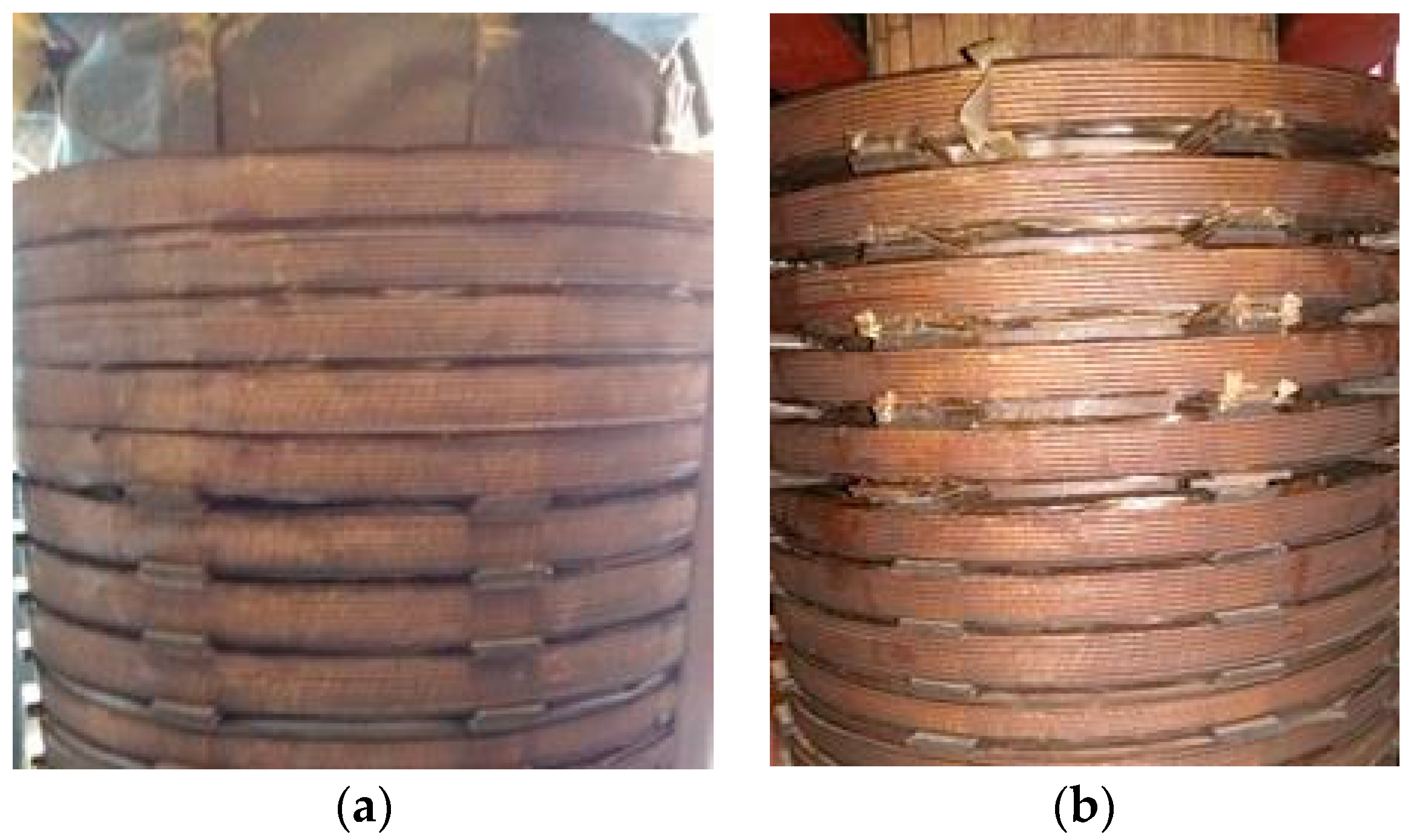
One of the research directions aimed at improving the interpretation of FRA transformer windings test results is conducting experiments with introduced controlled deformations. Their aim is to directly link a deformation or a short circuit in the winding with a change in the shape of the FRA curve. Though this approach seems fairly clear, deformation measurements are carried out very rarely, owing to the fact that this requires the transformer to be damaged. Another problem is the lack of data from the industry which would have been used to verify the results of frequency response measurements. There are very few examples of such experiments [1,7] and they take into account only a small range of deformation and/or are carried out on small transformers. The authors of this paper have performed measurements under conditions of controlled deformations on several transformers and used obtained FRA results for testing proposed data assessment approach. Other results used in this paper for verification of proposed new method come from the industry: comparison of sister units (the same type, with possible differences in constructional details) and influence of a tap changer position on FRA curves. Author’s experiences show that it is possible to introduce the new method of results assessment, based on simultaneous analysis of data coming from E2E and IntCap test setups [3,11,12,13].

To quantitatively assess the test results and propose new approach to data interpretation, the authors used several numerical indices. They are widely described in the literature [9,14,15,16,17,18,19,20,21,22], therefore only basic information of their application have been presented in

Table 1. Numerical indices used for assessment of test data [9,14,15,16,17,19,20,21,22].

Short Name	Full Name	Formula, [Reference]	Perfect Case 1
CC	Correlation Coefficient	$\mathrm{CC}=\frac{{{\displaystyle \sum }}_{i=1}^N{Y}_{0i}{Y}_{1i}}{\sqrt{{{\displaystyle \sum }}_{i=1}^N{\left[Y_{0i}\right]}^2{{\displaystyle \sum }}_{i=1}^N{\left[Y_{1i}\right]}^2}}$    [9,15]	1 ↓
ASLE	Absolute Sum of Logarithmic Error	$\mathrm{ASLE}=\frac{{{\displaystyle \sum }}_{i=1}^N\left|20lo{g}_{10}{Y}_{1i}-20lo{g}_{10}{Y}_{0i}\right|}{N}$  [17,22]	0 ↑
CSD	Comparative Standard Deviation	$\mathrm{CSD}=\sqrt{\frac{{{\displaystyle \sum }}_{i=1}^N{\left[\left(Y_{0i}-\overline{Y_0}\right)-\left(Y_{1i}-\overline{Y_1}\right)\right]}^2}{N-1}}$   [16]	0 ↑
ED	Euclidean Distance	$\mathrm{ED}=\sqrt{{{\displaystyle \sum }}_{i=1}^N{\left(Y_{0i}-Y_{1i}\right)}^2}$    [9,21]	0 ↑
SD	Standard Deviation	$\mathrm{SD}=\sqrt{\frac{{{\displaystyle \sum }}_{i=1}^N{\left(Y_{0i}-Y_{1i}\right)}^2}{N}}$      [14,19]	0 ↑
RMSE	Root Mean Square Error	$\mathrm{RMSE}=\sqrt{\frac{1}{N}{{\displaystyle \sum }}_{i=1}^N{\left[\frac{\left|Y_{0i}\right|-\left|Y_{1i}\right|}{\frac{1}{N}{{\displaystyle \sum }}_{i=1}^N\left|Y_{1i}\right|}\right]}^2}$   [15]	0 ↑
σ	Spectrum deviation	$\sigma =\frac{1}{N}{{\displaystyle \sum }}_{i=1}^N\sqrt{{\left[\frac{Y_{0i}-\left(\frac{Y_{0i}+Y_{1i}}{2}\right)}{\frac{Y_{0i}+Y_{1i}}{2}}\right]}^2+{\left[\frac{Y_{1i}-\left(\frac{Y_{1i}+Y_{0i}}{2}\right)}{\frac{Y_{1i}+Y_{0i}}{2}}\right]}^2}$ [15]	0 ↑
σs	Stochastic spectrum deviation	${\sigma }_s=\frac{100}{N}{{\displaystyle \sum }}_{i=1}^N\left|\frac{Y_{0i}-Y_{1i}}{Y_{1i}}\right|$      [15]	0 ↑
MM	Minimum-Maximum ratio	$\mathrm{MM}=\frac{{{\displaystyle \sum }}_{i=1}^N\min \left(Y_{0i},Y_{1i}\right)}{{{\displaystyle \sum }}_{i=1}^N\max \left(Y_{0i},Y_{1i}\right)}$      [16]	1 ↑
ρ	Normalized correlation coefficient	$\rho =\frac{{{\displaystyle \sum }}_{i=1}^N\left[\left|Y_{1i}\right|-\frac{1}{N}{{\displaystyle \sum }}_{i=1}^N{Y}_{1i}\right]\left[\left|Y_{0i}\right|-\frac{1}{N}{{\displaystyle \sum }}_{i=1}^N{Y}_{0i}\right]}{\sqrt{{{\displaystyle \sum }}_{i=1}^N{\left[\left|Y_{1i}\right|-\frac{1}{N}{{\displaystyle \sum }}_{i=1}^N{Y}_{1i}\right]}^2{{\displaystyle \sum }}_{i=1}^N{\left[\left|Y_{0i}\right|-\frac{1}{N}{{\displaystyle \sum }}_{i=1}^N{Y}_{0i}\right]}^2}}$ [15]	1 ↓
SSE	Sum Squared Error	$\mathrm{SSE}=\frac{{{\displaystyle \sum }}_{i=1}^N{\left(Y_{0i}-Y_{1i}\right)}^2}{N}$      [15,16]	0 ↑
SSRE	Sum Squared Ratio Error	$\mathrm{SSRE}=\frac{{{\displaystyle \sum }}_{i=1}^N{\left(\frac{Y_{1i}}{Y_{0i}}-1\right)}^2}{N}$       [20]	0 ↑
SSMMRE	Sum Squared Max-Min Ratio Error	$\mathrm{SSMMRE}=\frac{{{\displaystyle \sum }}_{i=1}^N{\left(\frac{\max (Y_{0i},Y_{1i})}{\min (Y_{0i},Y_{1i})}-1\right)}^2}{N}$    [15]	0 ↑

¹—value for identical datasets, the arrow indicates the direction of the value change as the deformation increases; where: Y₀—a reference set of data, Y₁—a set of compared data, $\overline{Y_0}$, $\overline{Y_1}$—arithmetic mean values of all summed values of a data set, N—total number of points.

. Formulas that are designed for assessment in one test setup only, e.g., from Chinese standard DL/T911-2004, which is to be used in end-to-end test setup, have been omitted. The main problem with application of indices for assessment of FRA test results is the lack of interpretation criteria: what values obtained from a formula application indicate a deformation. Some of presented indices are known to be inconsistent [22,23], which makes the assessment of FRA results difficult and equivocal if only one formula would be used. Therefore authors used 13 the most popular indices found in the literature. Table 1 presents short name, full name and formula, followed by its reference and the value obtained for the comparison of two identical datasets (perfect case). There is also added an arrow indicating whether the value increases or decreases with the increase of difference between compared values, which helps to understand the meaning of the numerical indices.

3. Cross Test Comparison Method

Two test configurations, presented at Figure 1, provide valuable information on the mechanical condition of windings. They are analyzed separately, as each of them is based on different phenomena present in windings—mainly capacitive and inductive couplings. For each test setup, various types of deformations have different influence on FR. Some faults in the active part will have stronger influence only on one test setup; others on both of them. In addition, when measurements recorded in a given test setup are compared between phases, there are always visible similar differences in LF range, both for end-to-end (E2E) and interwinding capacitive (IntCap) test setups. These changes are the result of various magnetic flux distribution, which for the middle column is symmetrical (via two side columns) and for side columns asymmetrical (via middle one and opposite side columns). The problem of a low frequency resonance position has been analyzed in [8]. Accordingly, comparison and assessment of curves measured for the same column may significantly reduce the influence of column geometry or specific constructional details (middle vs. side).

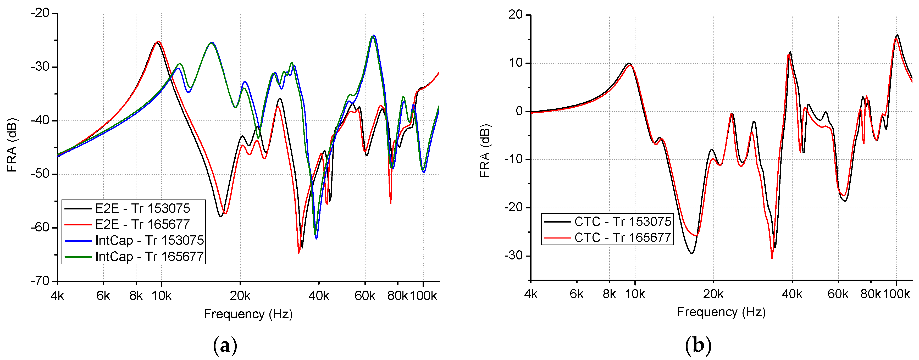
The Cross Test Comparison (CTC) method combines both the E2E and IntCap measurements into a single dataset, by subtracting the amplitudes at the corresponding frequencies. The resulting dataset is more sensitive in identifying deviations from baseline measurements (if compared to the reference data calculated in the same way). On the one hand, differences coming from two component curves are emphasized, which is expected due to subtraction result of two datasets. On the other hand, the new dataset shows changes in wider frequency range than single measurement, because E2E and IntCap show changes in curves in other frequencies for the same deformation.

CTC performed for each column will give three datasets (one for each phase), and these datasets subsequently may be compared together to provide additional information on the mechanical condition of transformer’s active part, not possible to obtain in the standard approach. An additional gain from the application of CTC is in reduction of the LF range difference in the shape observed for the middle column; also the impact of transformer’s specific construction on FR shape might also be reduced. An example of this effect may be difference between measurements performed on two side columns (A vs. C) in middle frequency range. Such results are expected to be similar, but still often show some deviations, observed in industrial results. The authors decided to use subtraction for CTC data, which makes it possible to keep the proper unit of resulting data, and there is no risk of signal intensification or suppression in given frequency points if multiplication or division functions would be used. If datasets are subtracted at frequency point, at which both E2E and IntCap have differences (if compared to the reference data), the resulting CTC value will provide more sensitive difference. If the difference will be present only for one input dataset (E2E or IntCap), the new CTC value will of course contain it. For CTC method test results are to be subtracted on the basis of the typical form of results presentation, which is the amplitude damping in the function of logarithmic frequency:

$$\mathrm{FRA}(\mathrm{dB})=20\log \frac{U_{out}}{U_{in}}$$

(1)

Such a form is the most popular way of presenting FRA results and most test devices use it as a standard method of data acquisition. The CTC can be thus defined as follows:

$$\mathrm{CTC}(f)={\mathrm{FRA}}_{\mathrm{E}2\mathrm{E}}(f)-{\mathrm{FRA}}_{\mathrm{CAP}}(f)$$

(2)

where FRA_E2E and FRA_CAP are the amplitudes of FR recorded in end-to-end open (E2E) and interwinding capacitive (IntCap) test setups, respectively. This approach makes it possible to juxtapose the influence of both voltage sides of a transformer and typical ranges of frequencies of both test setups in one graph. Observations made by the authors show that fault detection potential of two input test setups is additive, as each test setup behaves differently under influence of a given deformation.

An example of a CTC graph drawn using data presented on Figure 1 is given on Figure 2. The full frequency spectrum is presented, so it can be seen that natural difference between the phases is reduced in the LF range—curves have similar shape, but are shifted. This makes their comparison much easier. In the MF range the new curve contains differences observed for both E2E and IntCap curves, so it is easier to use automated assessment tools.

4. CTC Method Application and Results Assessment

Our CTC method was tested using data from measurements performed in three cases: a unit tested in laboratory with introduced controlled deformations; sister transformers measured under industrial conditions and a transformer with FRA changes resulting from tap-changer operations. All results have been presented below, with additional assessment by numerical indices already presented in Table 1. The graphical presentation of subsequent results on graphs, as well as their assessment, were done in MF range only, as this range is responsible for local deformations in windings; LF and HF ranges are usually omitted in industrial analysis.

4.1. Laboratory Tests

Laboratory experiments with deformations introduced into windings were carried out on an 800 kVA unit, 15/0.4 kV. The active part was untanked, and several types of deformations were introduced, resulting in several hundred curves recorded in E2E and IntCap test setups. Two deformations were chosen for analysis in this paper, which are presented on Figure 3, while their FRA results are presented in Figure 4 and Figure 5. They are respectively the effect of axial discs lowering (deformation 1) and axial discs expansion (deformation 2). The first deformation simulates loose winding with fallen off spacers and it was measured for five top discs lowered. The second one is possible when high axial forces in a winding have damaged the clamping system and it was measured also for five discs moved up.

The frequency range chosen for the analysis in both cases was from 20 kHz to 1.128 MHz (from inflextion point of increasing capacitive slope of the first resonance, to the half of remaining frequency range). The high value of the end of the MF range results from the small size of this unit, that was measured up to 20 MHz. The first deformation is analyzed in the

Table 2. Numerical indices results for laboratory tests—deformation 1 (frequency range 20 kHz–1.128 MHz).

Short Name	E2E	IntCap	CTC	Perfect Case
CC	0.999497	0.99956	0.9898	1 ↓
ASLE	0.226	0.253	2.56	0 ↑
CSD	1.954	1.296	2.041	0 ↑
ED	55.993	37.429	65.709	0 ↑
SD	2.133	1.426	2.503	0 ↑
RMSE	0.038	0.032	0.205	0 ↑
σ	0.018	0.02061	0.229	0 ↑
σs	2.565	2.969	31.517	0 ↑
MM	1.027	1.027	1.181	1 ↑
ρ	0.99985	0.99989	0.997	1 ↓
SSE	5.55	2.033	6.267	0 ↑
SSRE	1.26 × 10−3	1.26 × 10−3	1.602	0 ↑
SSMMRE	1.10 × 10−3	1.25 × 10−3	1.307	0 ↑

, which presents results of the indices application for these data.

In all cases, the formulas’ results showed that CTC data is the most sensitive indicator of changes between curves. It can be easily observed, when results are compared to the values from the last column, which contains perfect case comparison. Depending on the selected formula, the value was the smallest (e.g., CC or ρ, where the perfect condition is 1) or the biggest (the rest). The biggest differences are observed for: ASLE, RMSE, σ, σ_s, SSRE or SSMMRE, where CTC values change by an order of magnitude. Likewise, in comparison to standard test results (Figure 4a), the graphical presentation shows that CTC curves gave biggest differences between curves (Figure 4b). It can be seen on graph from 80 kHz to 600 kHz. The second example of the deformation—axial winding expansion is presented on graphs on Figure 5 and in the

Table 3. Numerical indices results for laboratory tests—deformation 2 (frequency range 20 kHz–1.128 MHz).

Short Name	E2E	IntCap	CTC	Perfect Case
CC	0.998761	0.99954	0.9747	1 ↓
ASLE	0.233	0.290	3.436	0 ↑
CSD	2.764	1.308	2.776	0 ↑
ED	72.825	45.17	81.082	0 ↑
SD	2.774	1.721	3.089	0 ↑
RMSE	0.05	0.037	0.315	0 ↑
σ	0.019	0.02359	0.351	0 ↑
σs	2.685	3.255	75.872	0 ↑
MM	1.028	1.031	1.218	1 ↑
ρ	0.99969	0.99988	0.991	1 ↓
SSE	7.697	2.961	9.542	0 ↑
SSRE	2.164 × 10−3	1.892 × 10−3	1.423	0 ↑
SSMMRE	1.765 × 10−3	1.655 × 10−3	3.597	0 ↑

.

Similarly to the previous deformation the CTC results show the biggest sensitivity for: ASLE, RMSE, σ, σ_s, SSRE or SSMMRE. These and the other numerical indices also in the case of CTC method show the biggest change of the value if compared to the E2E or IntCap results. The changes in graphs are in the similar frequency range as for deformation 1. It means that it is not possible to directly determine what type of deformation it is or to find its detailed location in the column. This conclusion is valid for all: E2E, IntCap and CTC datasets. Each transformer has it specific FR curve, so local changes in its geometry will be visible in similar frequency ranges, with similar character of changes (frequency shift and/or damping change). Further research on this problem will be performed by the authors.

4.2. Industrial Application—Sister Transformers

The two transformers compared in this point have same construction and are operated in the same station. These are 31.5 MVA, 110/33 kV units. They show differences in E2E and IntCap measurements, which may be the effect of a fault in an active part of one unit. From this reason they have been chosen as an example in this paper, because they can simulate two sets of measurements from one transformer after the deformation. The analyzed frequency range is as follows: 4 kHz–115 kHz. Data are presented in Figure 6 and

Table 4. Numerical indices results for sister units (frequency range 4 kHz–115 kHz).

Short Name	E2E	IntCap	CTC	Perfect Case
CC	0.998518	0.9995	0.97038	1 ↓
ASLE	0.284	0.202	5.948	0 ↑
CSD	2.317	1.227	2.573	0 ↑
ED	40.692	21.704	45.349	0 ↑
SD	2.319	1.237	2.584	0 ↑
RMSE	0.055	0.033	0.304	0 ↑
σ	0.023	0.016	0.765	0 ↑
σs	3.243	2.321	176.994	0 ↑
MM	1.036	1.024	1.549	1 ↑
ρ	0.99962	0.99987	0.98548	1 ↓
SSE	5.376	1.529	6.677	0 ↑
SSRE	2.45 × 10−3	1.01 × 10−3	64.682	0 ↑
SSMMRE	2.10 × 10−3	9.27 × 10−3	20.157	0 ↑

.

As in the previous case, all the formulas showed the biggest changes in CTC curve. It can be also seen on Figure 6 that application of the CTC reduced the frequency shift: changes are visible only as amplitude damping, and this makes visual detection and analysis much easier. These differences are observed in the frequency range 18 kHz–100 kHz. The good example is here the resonance at 18 kHz, that is shifted to the original frequency, but with many times bigger difference in damping. Application of CTC allows one to emphasize differences between these two units, which is helpful in the detection of a faulty transformer. The comparison of values in the table to the last column (perfect case) indicated that the biggest differences are for formulas: ASLE, RMSE, σ, σ_s, SSRE and SSMMRE: over an order of magnitude.

4.3. Industrial Application—OLTC Influence

The third CTC application example was carried out on data from transformer 10 MVA, 15.75/6.3 kV, for which FRA curves were recorded at various on-line tap changer (OLTC) positions. The frequency range in the 20 kHz–256 kHz. The results are presented in Figure 7 and in

Table 5. Numerical indices results for OLTC influence (frequency range 20 kHz–256 kHz).

Short Name	E2E	IntCap	CTC	Perfect Case
CC	0.98493	0.974	0.922	1 ↓
ASLE	0.994	1.215	4.652	0 ↑
CSD	7.954	5.503	9.633	0 ↑
ED	133.22	84.484	159.618	0 ↑
SD	8.709	5.523	10.435	0 ↑
RMSE	0.189	0.245	0.437	0 ↑
σ	0.08	0.098	0.317	0 ↑
σs	10.163	14.794	45.332	0 ↑
MM	1.12	1.169	1.354	1 ↑
ρ	0.99613	0.993	0.977	1 ↓
SSE	75.845	30.502	108.879	0 ↑
SSRE	0.062	0.033	13.358	0 ↑
SSMMRE	0.025	0.026	0.184	0 ↑

.

Once again, the biggest differences were exhibited for the CTC data by all formulas. Like in the two previous cases ASLE, σ, σ_s, SSRE and SSMMRE were especially sensitive, however the differences were smaller if compared to previous cases (Table 2 and Table 3). This is caused by the much bigger differences between the two curves in the E2E and IntCap test setups for the discussed example of OLTC influence. The differences between curves from 60 kHz to 100 kHz were highlighted, and there is a much bigger difference above 100 kHz.

5. Summary

The paper has outlined a new method for assessment of FRA test data. At present, only the curves measured at E2E test setup are the ones that are usually compared. IntCap data are also sometimes used, but separately and without connection to the E2E data. The paper proposes a method that combines these two test setups together in the one dataset. Both E2E and IntCap carry important information on the mechanical condition of the active part, but it is difficult to distinguish what changes between curves are responsible for the various types, locations and scales of deformations or other faults. Therefore, application of the CTC method makes it possible to use data obtained from both test setups in order to reach common conclusions.

Presented examples of measured transformers showed that CTC allows for amplification of the differences between curves. By introducing several numerical indices, it was possible to assess E2E, IntCap and CTC datasets. All the formulas showed that CTC is the most effective tool for detection of differences originating from possible faults. Most of the formulas have no interpretation criteria, as FRA curves recorded for various transformers are very different, and it is difficult to propose any specific values to unequivocally assess faults in the winding. Nevertheless, with CTC method application, the detection of such differences becomes easier, as all values of CTC presented in abovementioned examples were emphasized. From tested numerical indices the most sensitive to be used with CTC were: ASLE, RMSE, σ, σ_s, SSRE and SSMMRE. Their values significantly changed (by orders of magnitude) if compared to standard E2E or IntCap dataset. A conclusion may be drawn that their application for assessment of CTC data may be especially useful, by a rule of thumb.

Further research will be conducted on the detection ability of the CTC method e.g., location and type of fault. In the E2E and IntCap test setups the presence of similar faults in two different transformers may result in different influences on the FRA curve; there is different interaction of local geometry parameters and their influence on the curve shape. By performing tests of the CTC method for deformations in various transformers it may be found if its results provide a more direct correlation than E2E and IntCap. On the other hand, the presence of two different deformations in the same type of transformer may give similar changes to the original curve (cases of two different deformations from Section 4.1), so it will be difficult to distinguish the type and location of the fault.