An Energy Efficient Train Dispatch and Control Integrated Method in Urban Rail Transit


State Key Laboratory of Rail Traffic Control and Safety, Beijing Jiaotong University, Beijing 100044, China
*
Author to whom correspondence should be addressed.
Energies 2018, 11(5), 1248; https://doi.org/10.3390/en11051248
Submission received: 19 April 2018
/
Revised: 9 May 2018
/
Accepted: 9 May 2018
/
Published: 14 May 2018
Abstract
:With the rapid development of urban rail transit, the energy consumption of trains is increasing dramatically. The shortage of electrical energy is becoming more and more serious. In this paper, a novel method is proposed to better use regenerative braking energy for energy saving. A ‘time slot and energy grid’ model is set up to analyze the utilization of regenerative energy among trains. Based on this model, an energy efficient strategy that integrates train dispatch with train control is designed. The running time of trains in sections, the dwell time of trains at stations and the headway can be adjusted to find the global optimal solution for energy saving. The operational data of Beijing Changping subway line and Beijing Yizhuang subway line are used in simulation to illustrate the effectiveness of the proposed method in different scenarios. Simulation results show that our approach can significantly improve the utilization of regenerative braking energy and minimize the energy consumption in different scenarios when compared with the existing method.
1. Introduction
There are many advantages in urban rail transit such as high speed, punctuality, saving land, etc. It can effectively alleviate the traffic congestion problem of densely populated cities. However, the power consumption of urban rail transportation is very huge. Taking the Beijing subway line No.1 as an example, the gross energy consumption of the whole system is 147.51 million kWh in 2012, including 73.65 million kWh energy used for the traction of trains [1].
China is one of the major emitters of CO2 in the world [2] and the energy consumption of urban rail transit is very huge in China. Since the energy consumption of urban rail transit rises rapidly with the growth of the operating mileage, there is an increasing demand in reducing its energy consumption for sustainable development. The tractive energy of trains is the major component, accounts for more than 50% of the total energy consumption [1,3]. Most of the research focuses on reducing the tractive energy consumption while keeping trains running within the constraints of timetable.
The energy saving issue of urban rail transit has attracted the attention of many researchers in recent years. The existing technologies include methods associated with power feeding network [4,5] and approaches related to train regulation [3,6].
The possible techniques to improve the energy efficiency of the power feeding network are reviewed in [4]. They are classified into four categories, which are increasing supply capacity through deploying more supply positions, improving line receptivity for the absorption of regenerated energy, reducing losses in the feeding circuit and reducing distance the feeding current travels. Kondo [5] categorizes the existing energy saving technologies in the railway vehicle traction field into two domains. One is the reduction of the loss in traction equipment through employing more energy efficient equipment or through improving traction control. The other is increasing the regenerative energy by regenerative brake control or by applying energy storage devices.
Gonzalez-Gil et al. [6] present an overview of the technologies for recovery and management of regenerative energy in urban rail transit, covering timetable optimization, onboard and wayside energy storage system and reversible substations. In another paper [3], they give a comprehensive appraisal of the main technologies currently available to minimize the energy consumption of urban rail transport, includes regenerative braking, energy efficient driving, traction losses reduction, energy metering, smart power management, and so on.
The existing energy saving methods related to train regulation can be subdivided into three categories, the optimal train driving method, the energy efficient timetable method and the train dispatch and control integrated method. The optimal train driving method minimizes the tractive energy consumption of a train within the constraint of timetable through selecting the optimal control strategy, which is determined by the number and positions of switches of the train’s working conditions [7,8,9,10,11,12,13,14,15]. The energy efficient timetable method makes use of regenerative energy to reduce the tractive energy consumption of trains. It synchronizes the acceleration and deceleration of different trains in the same electrical section through an elaborately designed timetable [16,17,18,19,20,21,22]. Usually, the synchronization is realized through adjusting the headway and the dwell time of trains at stations. The departing train can use the regenerative energy of the arriving train for traction. To further improve the utilization of regenerative energy and reduce the tractive energy consumption, a new kind of method has been researched deeply recently, which integrates train dispatch with train control [23,24,25,26,27]. In addition to the headway and the dwell time of trains at stations, the integrated method modifies the running time of trains in sections to synchronize the deceleration and acceleration of trains and maximize the utilization of regenerative energy.
In this paper, we propose an energy efficient train dispatch and control integrated method. A ‘time slot and energy grid’ model is proposed to analyze the utilization of regenerative energy among multiple bidirectional running trains in the same electrical section. Based on the model, a unified energy efficient integrated strategy is designed to improve the utilization of regenerative energy and reduce the tractive energy consumption of trains. At last, the operational data of Beijing Changping subway line and Beijing Yizhuang subway line are used in simulation to illustrate the performance of the proposed method in long section and short section, respectively. According to the simulation results, it can be concluded that the proposed method can obviously reduce the total tractive energy consumption in different scenarios and have little impact on the operation of urban rail transit.
The rest of this paper is organized as follows. In Section 2, we review the literature on the energy saving methods related to train regulation, the defects of each kind of methods are analyzed. A ‘time slot and energy grid’ model is proposed to analyze the utilization of regenerative energy in Section 3. Based on the model, the energy efficient train dispatch and control integrated method is designed. In Section 4, the objective function and the optimization model are formulated. In Section 5, the operational data of Beijing Changping and Beijing Yizhuang subway lines are used in simulation to illustrate the effectiveness of the proposed method in different scenarios. Finally, our work is concluded in Section 6.
2. Related Works
In this section, the research on energy saving methods related to train regulation is reviewed. The defects of each kind of method are analyzed.
2.1. The Optimal Train Driving Method
The optimal train driving method searches for the optimal control strategy to minimize the tractive energy consumption of the train within the constraints of timetable. Su et al. [7] propose a numerical algorithm to avoid unnecessary switches between the acceleration and braking of a train and reduce the tractive energy consumption during switches. Wong et al. [8,9] use a genetic algorithm (GA) in searching for the optimal number and locations of coasting points to minimize the energy consumption. Chang et al. [10] generate a coasting control table for a train to decide the exact time to start coasting and to resume motor control. Bocharnikov et al. [11] investigate the effects of coasting strategy, acceleration and braking performance on the energy consumption and running time of a train. They use GA and fuzzy set to seek the optimal solution to minimize the energy consumption within the constraints of timetable. Ding et al. [12] adjust the number and positions of coasting points, and the running time of a train in sections, within the constraint on the total running time, to minimize energy consumption. Tian et al. [13] analyze the power flows from substations under different speed profiles, optimize the driving strategy through evaluating the total energy consumption from substations. Milroy et al. [14] analyze the experiences of excellent train drivers and search for the most energy saving transition points of working conditions. Within a given journey time, Howlett et al. [15] use the Pontryagin principle to determine the optimal switching points in the continuous control problem, and use the Kuhn–Tucker equations to find the optimal switching times in the discrete control problem.
Although the optimal train driving method can find the control strategy to minimize the energy consumption of a single train, it can not effectively reduce the total tractive energy consumption of all the trains without considering the utilization of regenerative energy. The speed profile generated by the optimal driving strategy may not be beneficial for the utilization of regenerative energy among trains.
2.2. The Energy Efficient Timetable Method
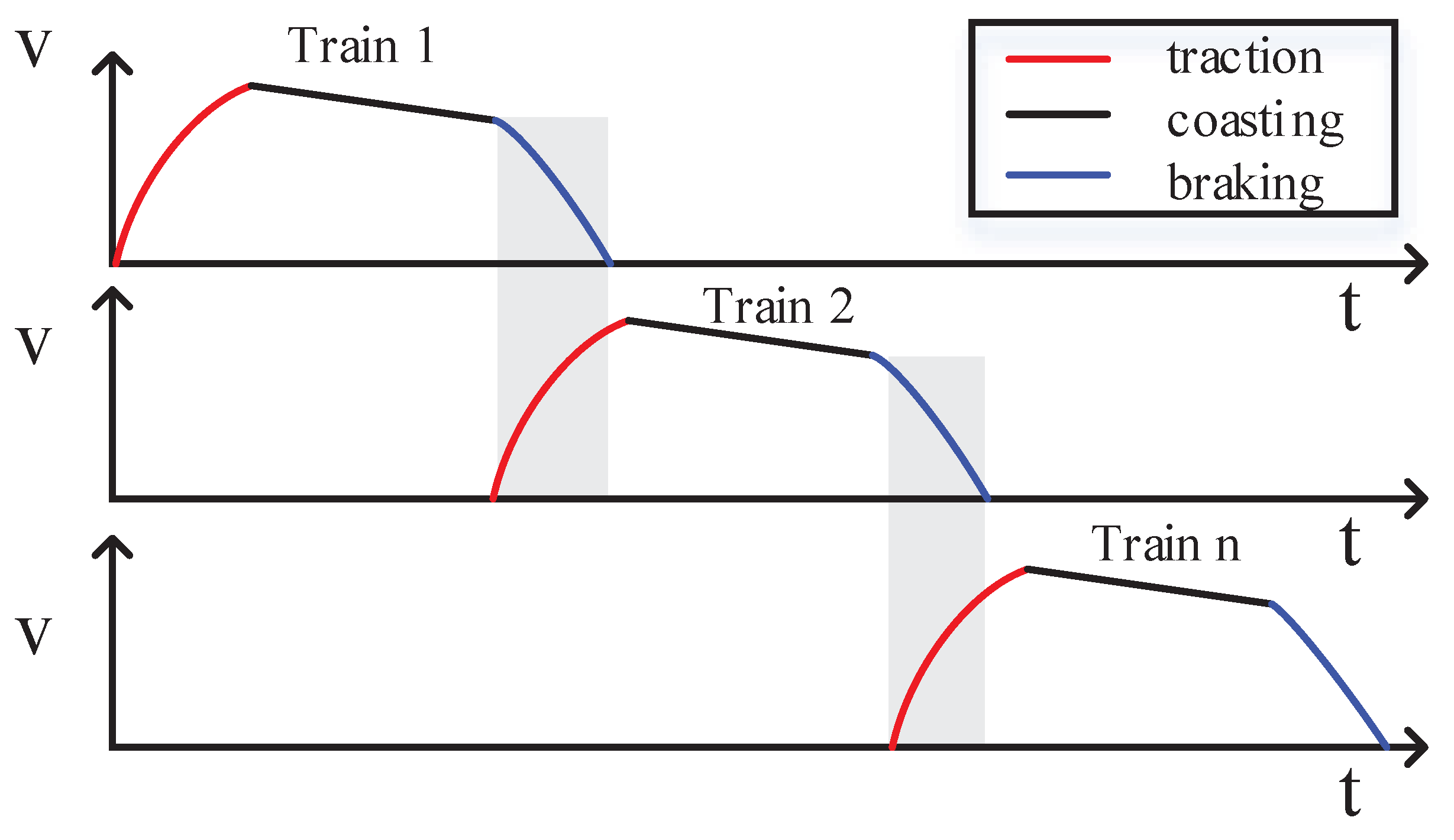
The energy efficient timetable method, illustrated in Figure 1, synchronizes the acceleration and deceleration of different trains through an elaborately designed timetable to utilize regenerative energy and minimize the tractive energy consumption of all the trains.
Gong et al. [16] obtain the optimal energy efficient timetable through modifying the dwell time of trains. Furthermore, they propose adjusting the driving speed and coasting time of a disturbed train to adapt the established timetable under disturbances. Yang et al. [17,18] use GA to maximize the overlapping time between adjacent accelerating and decelerating trains and shorten the waiting time of passengers through adjusting the headway and the dwell time of trains at stations. Pena et al. [19] synchronize the brake and acceleration of trains in the same electrical section through controlling the arriving and departing time of trains at stations, in order to maximize the utilization of regenerative energy. Li et al. [20] apply a fuzzy multi-objective optimization approach to solve a train scheduling model to minimize the energy consumption and carbon emission as well as the total waiting time of passengers. Albrecht et al. [21] propose a method to reduce the power peak and energy consumption for a given headway and synchronization time through controlling the running time of the train. Nasri et al. [22] study the effects of headway and reserve time on energy consumption and propose a method to determine the optimal timetable for maximum usage of regenerative energy at stations. It is proved that the simultaneous presence of braking and accelerating trains within the same electrical section in the case of big headway is quite rare.
The energy efficient timetable method can use the regenerative energy to reduce the tractive energy consumption. Usually, the optimal speed profile that minimizes the tractive energy consumption of a train is adopted, which may not be beneficial to the utilization of regenerative energy. Although the headway has a great impact on the energy consumption, it is not a flexible factor. Its upper limit deals with the quality of transportation and the lower limit depends on technical and economic aspects [22]. Furthermore, the dwell time is adjusted together with the headway, which has a bigger impact on the satisfaction of passengers than the adjustment of running time [21].
Some researchers set up models to analyze the synchronized time between accelerating and braking trains [16,17,18,19,20] and calculate the regenerative energy consumption during the synchronized time. The model to analyze the regenerative energy consumption among multiple bidirectional running trains in different electrical sections is very complicated, which is the ideal case for the utilization of regenerative energy. Many researchers make some simplifications, such as only considering the utilization of regenerative energy among adjacent trains, to make the problem tractable. Some researchers resort to commercial simulation tools to get the optimal timetable [19,21,22]. To solve the problem of dimensionality, some simplifications are also made by researchers, such as dealing only with trains that are relatively close together.
2.3. The Train Dispatch and Control Integrated Method
The train dispatch and control integrated method improves the usage of regenerative energy through adjusting the headway, the dwell time of trains at stations and the speed profiles of trains in sections, simultaneously. Through selecting different speed profiles, the running times of a train in sections are adjusted.
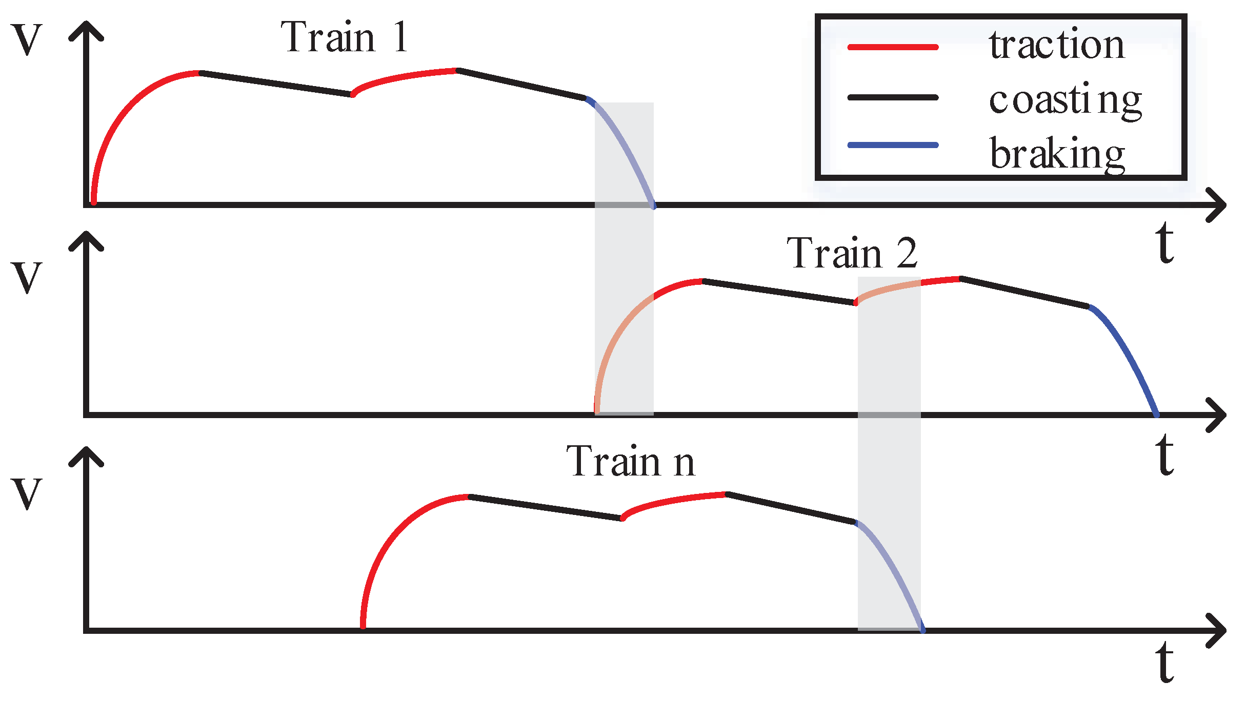
Bu et al. [23] set up a model for the design of energy efficient timetable, which coordinates the adjacent accelerating and decelerating trains through adjusting the headway, the tractive, cruising, coasting, braking and dwell time of trains to improve the usage of regenerative energy and reduce the tractive energy consumption. Su et al. [24] develop an analytical formulation to calculate the optimal speed profile within the constraint of a given running time of each section. A numerical algorithm is designed to distribute the total trip time among different sections and generate the integrated timetable, which includes both timetable and speed profiles, to achieve energy efficient operation. A numerical algorithm is put forward in [25] to calculate the optimal driving strategy within a given trip time. A model to efficiently use the regenerative energy for energy saving is formulated, which coordinates the control of trains through adjusting the departure time of trains at stations.Chen et al. [26] propose an approach to mitigate the delay of trains and decrease the energy consumption of trains simultaneously through adjusting the time table and speed profiles. As shown in Figure 2, Chen et al. [27] propose a ‘two-time traction’ control strategy. A train traveling in long sections can use the regenerated energy of braking trains for the 2nd traction. Since the utilization of regenerative energy is not limited in the station area, the method has a better energy efficiency than other integrated methods in the case of long section. In this paper, it is selected as the existing method for performance comparison with the proposed method.
The integrated method introduces the factor of speed profile to improve the usage of regenerative energy, and it has a better energy saving effect than the energy efficient timetable method. Due to the introduction of speed profiles, the analytical model of the integrated method is even more complicated than that of the energy efficient timetable method. In this paper, a simplified analytical model is set up to reduce the time, resources and expertise required to design the optimal timetable. Both the energy efficient timetable and the integrated method can benefit from the simple and efficient analytical model.
3. The Proposed Energy Efficient Integrated Method
In this section, we first define some concepts. Then, we present the time slot and energy grid model to analyze the usage of regenerative energy. After that, we give the energy efficient train dispatch and control integrated method.
3.1. Definitions
Before introducing the energy saving methods, it is necessary to define the following concepts:
- -
- Short section: a train can travel across a section within a given trip time though one time of traction;
- -
- Long section: a train needs at least two times of traction to run through a section within a given trip time;
- -
- The tractive energy (TE): the energy needed for traction by all the trains on the line;
- -
- The tractive energy consumption (TEC): the energy drawn from the substations for traction by all the trains;
- -
- The regenerative energy (RE): the regenerative energy generated by all the trains;
- -
- The regenerative energy consumption (REC): the regenerative energy consumed by all the trains.
TE can be calculated as
3.2. The Time Slot and Energy Grid Model
A typical scenario of urban rail transit is illustrated in Figure 3, multiple bidirectional running trains travel in different electrical sections of a line. The line is divided into k electrical sections, n trains are running on the line. It has
where and are the number of trains within the ith electrical section in the up and down directions, respectively.
Due to the limitations of the existing integrated method, trains can only use the regenerated energy of the adjacent braking trains in the same direction and within the same electrical section. For example, in Figure 3, the train can only use the regenerative energy of the or the train, when it is in the same electrical section as the or the train, and its traction time overlaps with the braking time of the train or that of the train. The existing methods constrain the utilization of regenerative energy and seriously impact the effect of energy saving.
The ideal situation for the utilization of regenerative energy is that a tractive train can use the regenerated energy of any braking trains in the same electrical section. For example, in Figure 3, the and the train can use the regenerated energy of the train. Due to the complexity of the analyzing model, the existing methods can not analyze the utilization of regenerative energy in the ideal situation and develop an optimal strategy for energy saving. In this paper, we propose a ‘time slot and energy grid’ model, which can analyze the usage of regenerative energy among multiple bidirectional running trains in the same electrical section. Based on the model, an energy efficient train dispatch and control integrated method is developed.
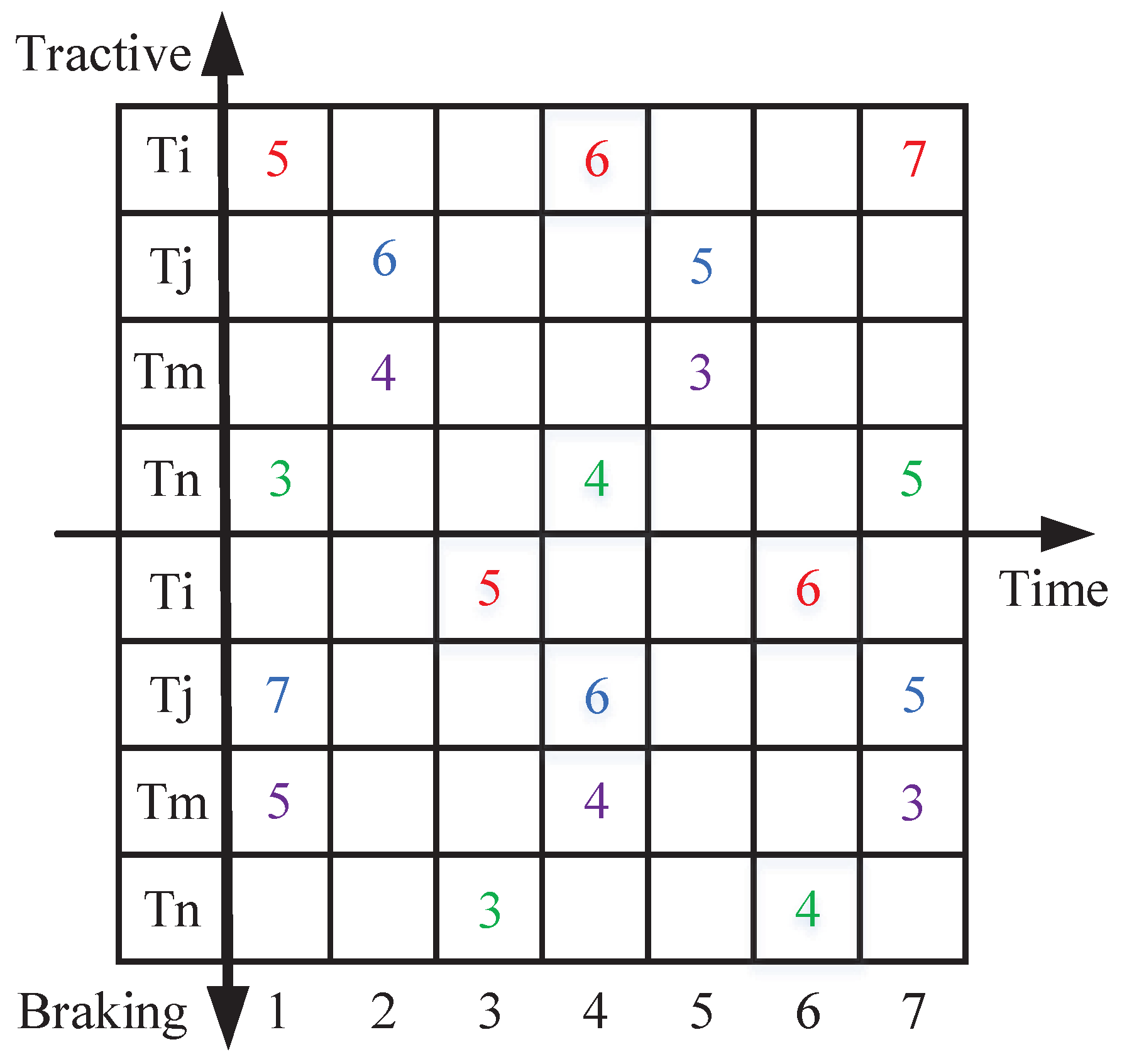
The model is illustrated in Figure 4. It is assumed that the first train starts running at the 0 moment, and the last train stops running at the T moment. The total running time is divided into K time slots. The length of each time slot is dt. It has d. Every slot can be vertically divided into a column of grids. Each train has two rows of grids. One row of grids are above the horizontal axis, which indicate the tractive energy needed by the train in each time slot. Another row of grids are below the horizontal axis, which indicate the regenerative energy created by the train. Since each grid denotes the tractive or regenerative energy of a train in a time slot, it is named as ‘energy grid’ in this paper.
If dt is small enough, it can be assumed that the working condition, the tractive (braking) force, the velocity, the basic and the additional resistance of a train remain unchanged within an energy grid. Accordingly, the resultant force of a train, which is the sum of the tractive (braking) force, the basic resistance and the additional resistance of the train, also keeps unchanged within an energy grid. The assumption significantly simplifies the analysis of energy consumption and makes the analysis of regenerative energy utilization in the ideal situation possible without affecting the credibility of the analysis results. The errors introduced by the assumption can be ignored provided that dt is small enough.
As shown in Figure 4, four arbitrary trains are selected as an example to analyze the usage of regenerative energy among multiple bidirectional running trains. Each train has two energy grids per time slot that are distributed on both sides of the horizontal axis. The contents of the two energy grids indicate the position and working condition of a train in the time slot. If there is a number in the energy grid above the horizontal axis, it means that the train is in tractive condition. If the number is in the energy grid below the horizontal axis, it means that the train is in braking condition. If neither of the grids has content, the train is stopping or in coasting condition, no energy is consumed or generated by the train. The number in either of the grids indicates that the electrical section the train is traveling within at the time slot.
The numbers below the horizontal axis denote the sequence of the time slots. For ease of illustration, we reduce the number of time slots between different working conditions of trains. The time slots are not continuous in time. As shown in Figure 4, from the first to the seventh time slot, the sequence of working conditions of the train is
where T and B indicate the tractive and braking conditions of a train, respectively. The symbol C represents the stopping or coasting conditions of a train.
As we can see in Figure 4, in the 1st time slot, the and train are in tractive condition, the and train are in braking condition. Since both the and the train are in the 5th electrical section, the train can use the regenerative energy of the train. Similarly, the regenerated energy of the train can be used by the train in the 4th time slot. The train can use the regenerative energy of the train in the 7th time slot.
3.3. Energy Efficient Integrated Strategy
Based on the proposed time slot and energy grid model, we develop a unified energy efficient integrated strategy for both ‘short section’ and ‘long section’ scenarios. Unlike the existing integrated methods, the number of times of train traction in a section is not restricted to one or two times. It depends on the timetable specified running time of the section, the parameters of the line and the train.
A group of speed profiles are generated for both up and down directions of each section. The time difference between the running time of the timetable and that of each profile is kept within a predefined range. To be consistent with the actual operation of urban rail transit, different trains use the identical speed profile in the same direction of a section. Each tractive train can use the regenerated energy of any braking train within the same electrical section.
Since it is assumed that the working condition, the resultant force and the velocity of a train remain unchanged in an energy grid, the power of a train in an energy grid, which is the product of the resultant force and the velocity of the train, is also constant. No integration is needed to calculate the tractive (regenerative) energy of an grid.
In each time slot, a tractive train can use the regenerated energy of any braking train within the same electrical section. The tractive energy (TE) and the regenerative energy (RE) of the same electrical section are summed, respectively. The results of summation are compared. The smaller one equals to the regenerative energy consumption (REC) of the electrical section. The TE and the REC of the time slot are the summation of the TE and the REC of each electrical sections, respectively. The TE and the REC are the summation of the TE and the REC of every time slots, respectively. The TEC is the difference between the TE and the REC:
The distinct features of our method are as follows:
- -
- The utilization of regenerative energy among multiple bidirectional running trains within the same electrical section is considered.
- -
- The actual division of electrical sections and the additional resistance of a train are considered, which make the results more realistic.
- -
- No limitation on the times of train traction in a section is needed. The utilization of regenerative energy can take place anywhere in sections.
- -
- A unified strategy is designed for both short section and long section scenarios.
- -
- The mutual constraints among the headway, the running time and the dwell time of trains are loose.
- -
- The proposed method is more energy efficient than the existing method in different scenarios.
An algorithm is designed to find the optimal combination of the headway (optional), the speed profiles of trains in sections and the dwell time of trains at stations, with the minimum TEC.
4. Energy-Saving Optimization Model
In this section, firstly, the parameters used in the energy saving optimization model are introduced. Then, the objective function is defined to minimize the TEC. After that, the energy saving optimization model is formulated.
4.1. Parameters
Different parameters are defined for the up and down directions. The symbols without and with hat represent parameters of the down and up directions, respectively. The parameters with letter ‘i’ in subscript indicate that they belong to the section or the station. The symbols with letter ‘i,j’ in subscript represent parameters pertain to the speed profile of the section. Those with ‘k’ in the bracket mean that they are parameters of the slot. The parameters used in our model are introduced as follows:
| the number of speed profiles of the ith section; | |
| the timetable specified running time of trains in the ith section; | |
| the running time of the ith section when the jth speed profile is adopted; | |
| the number of time slots of the running time in the ith section when the jth speed profile is adopted; | |
| the dwell time of trains at the ith station; | |
| the number of time slots of the dwell time at the ith station; | |
| the time slot that the train departs from the ith section; | |
| the time slot at the end of the down, up directional running; | |
| the headway; | |
| the number of time slots of the headway; | |
| the turn back time; | |
| the number of time slots of the turn back time; | |
| the tractive force of a train (in KN) at the kth time slot of the ith station when the jth speed profile is adopted; | |
| the braking force of a train at the kth time slot (in KN); | |
| the basic resistance of a train at the kth time slot (in KN); | |
| the starting resistance of a train at the kth time slot (in KN); | |
| the additional resistance of a train at the kth time slot (in KN); | |
| the running resistance of a train at the kth time slot (in KN); | |
| the resultant force of a train at the kth time slot (in KN); | |
| , | the mass of a motor car (in tons); |
| , | the mass of a trailer car (in tons); |
| , | the number of cars of a train; |
| g, | the equivalent additional slope of the line; |
| , | the speed of a train at the kth time slot if the jth speed profile of the ith section is adopted; |
| , | the position of a train at the kth time slot if the jth speed profile of the ith section is adopted; |
| , | the acceleration of a train (in ) at the kth time slot; |
| , | the rotary mass coefficient; |
| m, | the mass of a train (in tons); |
| , | the energy needed for traction by all the trains at the kth time slot; |
| , | the conversion efficiency coefficient of the tractive energy; |
| , | the regenerative energy generated by all the trains at the kth time slot; |
| , | the conversion efficiency coefficient of the regenerative braking energy; |
| , | the consumed regenerative energy by all the trains at the kth time slot; |
| , | the tractive energy consumption at the kth time slot; |
| , | the sum of the TEC of each time slot; |
| , , | the starting position, the ending position of the zth electrical section; |
| , , | the minimum running time of trains in the ith section; |
| , | the adjustment rang of running time; |
| , , | the minimum dwell time of trains at the ith station; |
| , , | the maximum dwell time of trains at the ith station; |
| , | the speed limitation of the line at the position ; |
| , | the speed limitation of the train; |
| D, | the length of the line; |
| , | the average traveling speed of a train (in km/h); |
| , | the vector of running time; |
| , , , | the number of extended, unchanged and shortened running time; |
| , | the vector of dwell time; |
| , , , | the number of extended, unchanged and shortened dwell time. |
4.2. Definition of the Objective Function
The TE of a train contains two parts. One part is provided by substations of the electrical sections on the line, which is called TEC of the train. Another part is the consumed regenerative energy provided by other trains, namely REC of the train. The total TE and the total REC are the sum of each train’s TE and the sum of each train’s REC, respectively. The total TEC equals to the difference between the total TE and the total REC. The primary objective of the energy-saving optimization model is to minimize the total TEC through maximizing the total REC.
To find the optimal solution, the running time of trains in sections, the dwell time of trains at stations and the headway (optional) are adjusted to improve the utilization of regenerative energy and reduce the tractive energy consumption. Firstly, based on the parameters of the line and the train, a group of speed profiles are generated for the up and down directions of each section, respectively. Each speed profile represents an option of running time for the section.
Secondly, based on the selected speed profiles, the operation status of the first train in any time slot can be got. Then, combined with the headway, the status of all the other trains in any time slot can be deduced. Furthermore, through using the proposed ‘time slot and energy grid’ model, the total TE, RE , REC and TEC can be calculated.
Lastly, genetic algorithm is adopted to find the optimal solution of the model. The combination of the selected speed profiles of sections, the dwell time of trains at stations and the headway (optional) with the minimum total TEC is adopted to design the energy efficient timetable.
A typical subway line is illustrated in Figure 5. Assuming that there are M stations, L electrical sections and N trains on the line. The total simulation time, T, is divided into K time slots. For a train running in the down direction, if the jth speed profile of the ith section is adopted, the resultant force applied to the train in the kth slot can be expressed as
The tractive and braking force of a train depend on its working conditions. It has
When the speed of a train is lower than 5km/h, the resistance of the train is composed of the starting resistance and the additional resistance. Otherwise, the resistance of the train comprises the running resistance and the additional resistance. The resistance of the train can be expressed as:
The starting resistance of the train can be calculated as
The running resistance of the train can be calculated as
It should be noted that the starting resistance and the running resistance of a train depend on the characteristics and speed of the train. The coefficients in Equations (6) and (7) are obtained from the train manufacturer of the Beijing Yizhuang and Beijing Changping subway lines. For other kind of trains, the coefficients in the above-mentioned equations may be different.
The additional resistance of the train, which includes the grade resistance, the curve resistance and the tunnel resistance, depends on the parameters of the line. It can be calculated as
The speed profiles of a train in sections can be obtained through using the kinetic equations. The position, the speed and the acceleration of the train are calculated as follows:
Similarly, we can get the resultant force, the running resistance, the position, the speed and the acceleration of a up direction running train in the kth time slot when the jth speed profile of the ith section is adopted, which are represented respectively as , , and , where .
The speed of the first train running in down direction at the kth time slot can be represented as
where
To keep the coordinate of the up direction consistent with that of the down direction, the train position in the up direction is calculated as
Similarly, the speed of the first train running in the up direction at the kth time slot can be expressed as
where
The speed of the first train at the time slot is
where
Taking the operational characteristics of urban rail transit into consideration, it can be assumed that different trains adopt the identical speed profile in the same direction of a section. Then, based on the given headway, , we can calculate the speed of the nth train at the kth time slot as follows:
where , .
Similarly, we can get the tractive force, the braking force, the position of the nth train at the kth time slot, which are represented as , and , respectively. Through using the ‘time slot and energy grid’ model, the TE, RE, REC and the total TEC can be calculated.
The TE of the kth time slot can be expressed as
The RE of the kth time slot is
The equation to calculate the REC of the kth time slot goes here:
The value of depends on the position of the nth train in the kth time slot. It has
The model is used to minimize the total TEC. The objective function can be defined as
4.3. Energy Saving Optimization Model
The total TEC depends on the running time of trains in sections, the dwell time of trains at stations and the headway. We take the total TEC as the objective of optimization and formulate the energy saving optimization model as follows:
The constraints in Equation (22) are explained as follows:
- (1)
- The constraint on the running time of trains in the up direction of the ith section.
- (2)
- The constraint on the difference between the adopted running time and the timetable specified running time in the up direction of the ith section.
- (3)
- The constraint on the dwell time of trains in the up direction at the ith station.
- (4)
- The constraint on the running time of trains in the down direction of the ith section.
- (5)
- The constraint on the difference between the adopted running time and the timetable specified running time in the down direction of the ith section.
- (6)
- The constraint on the dwell time of trains in the down direction at the ith station.
- (7)
- The constraint on the speed of a train.
- (8)
- The constraint on the position of a train.
Although some simplifications related to the power network have been made in the proposed model, such as the power network layout, the transmission loss and the voltage limits, the proposed method should be more energy efficient due to improved usage of regenerative energy when compared with the existing method under the same conditions. The effect of energy saving is related to the parameters of the power network, which will be considered in our future work. Further work will also include full validation to determine whether the improved usage of regenerative energy is realistic.
5. Simulation and Discussion
In this section, we use the operational data of Beijing Changping subway line and Beijing Yizhuang subway line in simulation to illustrate the effectiveness of the proposed method for ‘long section’ and ‘short section’ scenarios, respectively.
5.1. The Genetic Algorithm Used in Simulation
Genetic algorithm (GA) is a method to search for the optimal solution by simulating the natural evolutionary process. It has been widely applied to the research of energy saving [28,29,30] and the research of transportation system [31,32,33,34,35]. In this paper, the GA toolbox of Matlab (7.0, The MathWorks Inc., Natick, MA, USA) is used to find the global optimal solution of the optimization model given in Equation (22). The objective function of Equation (22) is taken as the fitness function.
The operational data of Beijing Changping subway line are used in simulation to illustrate the performance of the proposed method in ‘long section’ scenario. The parameters of GA are listed as follows. The crossover rate, the mutation probability and the population size are 0.8, 0.2 and 200, respectively. The fitness function has 25 parameters that depend on the number of stations on the line. The maximum number of iterations is set to 100 times the number of parameters of the fitness function. The algorithm is terminated when it reaches the maximum number of iterations or the average relative changes in the best fitness value over the last 50 generations are less than or equal to 1E-6.
Furthermore, we use the parameters of Beijing Yizhuang subway line to illustrate the performance of the proposed method in a ‘short section’ scenario. The following parameters are adopted in the GA. The crossover probability, the mutation probability and the population size of GA are the same as those used in the ‘long section’ scenario. There are 53 variables in the fitness function. Accordingly, the maximum number of iterations is 5300. The stop criterion of the algorithm is the same as that of the ‘long section’ scenario.
5.2. Simulation of Long Section Scenario
The operational data of Beijing Changping subway line (BJCP) are used in the simulation of long section scenarios. There are seven stations, six electrical sections and 20 trains. The mass of each fully loaded train is 294.6 tons. The length of the six sections are as follows:
Among these sections, there are three short sections and three long sections. The currently adopted headway is 240 s, which is used in simulation to illustrate the performance of the energy saving methods in the case of long section and big headway. Furthermore, we use a 90 s headway in simulation to illustrate the effectiveness of the methods in a long section and small headway scenario. One round trips of 20 trains are simulated. When the last train returns to the 1st station, the simulation is terminated.
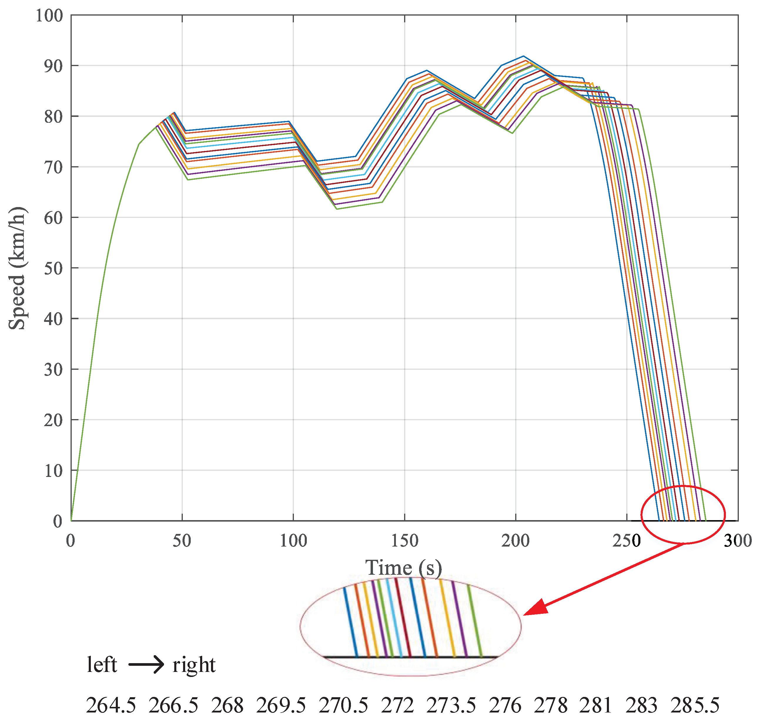
Firstly, a group of speed profiles are generated for each section in both up and down directions. The speed profiles represent variable control strategies and different running time of trains in each section. To reduce the impact of the energy saving method on operation and improve its applicability, the differences between the running time of the profiles and that specified by timetable are kept within s. As an example, Figure 6 illustrates the 12 different speed profiles in the down direction of the first section.
Secondly, the dwell time of trains at stations are adjusted together with the running time to synchronize the acceleration and deceleration of trains in the same electrical section, improve the utilization of regenerative energy and minimize the total TEC. The timetable specified dwell time of Beijing Changping subway line is between 30 s and 50 s. To reduce the impact of energy saving method on the transfer of passengers at stations, the dwell time of trains at stations is limited within the range of .
There are 25 genes in the chromosome. The 1st–6th genes represent the indexes of the selected speed profiles of the 1st–6th sections in the down direction, respectively. The 7th–12th genes stand for the dwell time of trains at the 2nd–7th stations in the down direction, respectively. Since the dwell time of trains at the 1st station is contained in the headway, it is not considered here. The 13th–18th genes denote the indexes of the adopted speed profiles of the 1st–6th sections in the up direction, respectively. The 19th–24th genes represent the dwell time of trains at the 2nd–7th station in the up direction, respectively. The last gene indicates the headway. Since it is not a flexible factor, we keep it unchanged in the simulation.
Lastly, the vectors of lower bounds and upper bounds for the iterations of GA are defined as
where A is the vector of lower bounds, B is the vector of upper bounds, and represents a array of ones.
The curve with the minimum index, ‘1’, has the shortest running time in the section. The curve with a larger index has a longer running time. In the simulation, since we generate 12 curves for each section, the curve with index ‘12’ has the longest running time. The minimum and the maximum dwell time of trains at stations in both directions are 25 s and 55 s, respectively. The lower bound and the upper bound of headway are set to the same value, 240, which means that the headway will not be adjusted for energy saving.
Through using GA, we find the global optimal solution, a combination of the speed profiles in sections, the dwell time of trains at stations and the headway (optional), with the minimum total TEC. For the simulation of long section big headway scenario, the optimal chromosome is
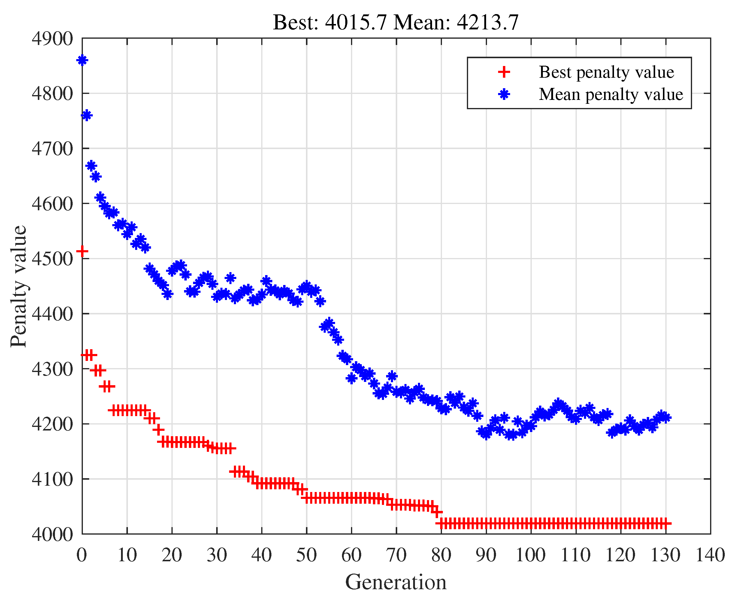
The best and the mean penalty value of each generation is illustrated in Figure 7. The GA terminates at the 130th generation. The best and the mean penalty value of the last iteration are 4015.7 and 4213.7, respectively.
For the simulation of long section small headway scenario, the best chromosome is
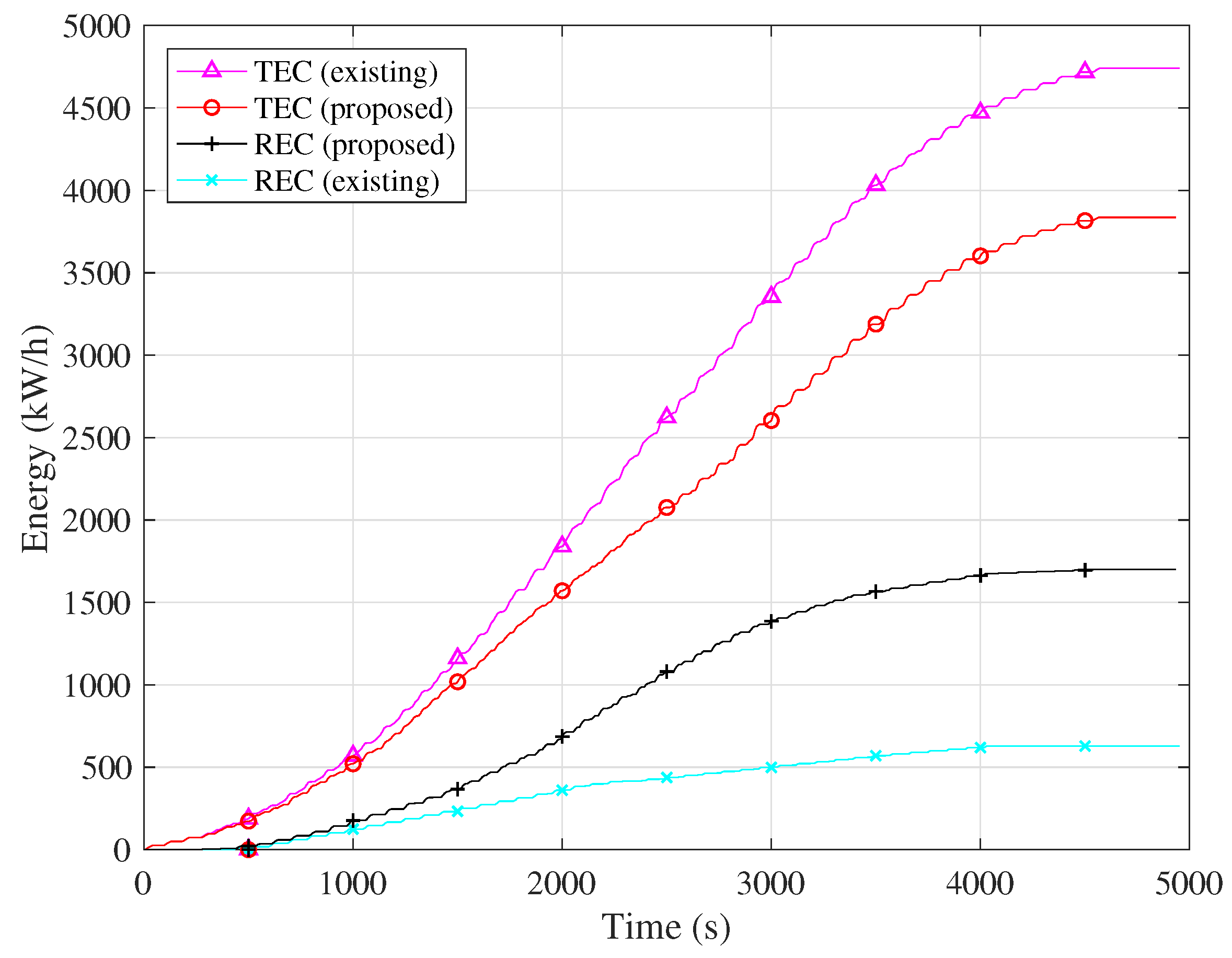
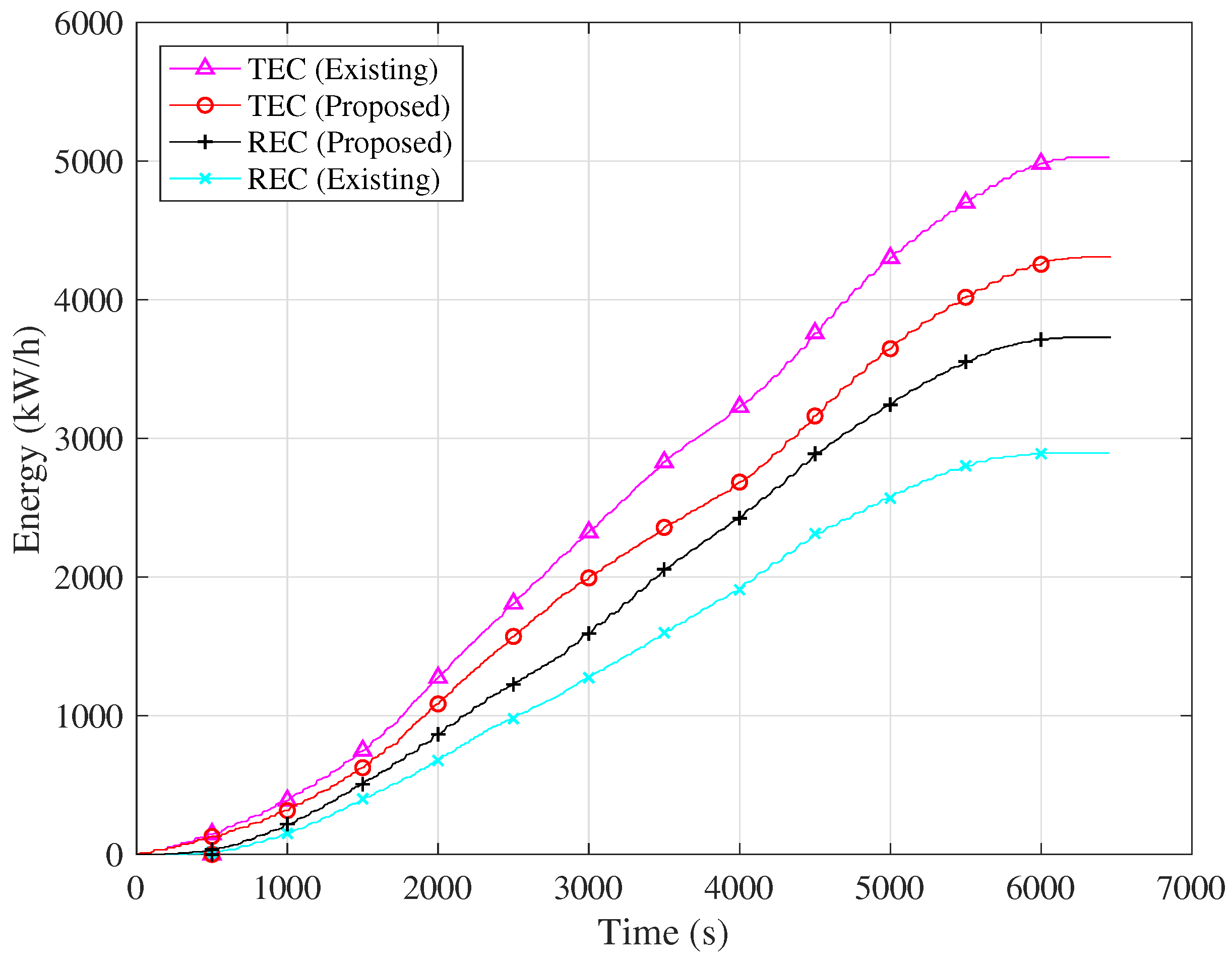
The train dispatch and control integrated approach proposed in [27] is selected as the existing method for performance comparison with the proposed method. The energy consumption of the existing and the proposed methods in long section big headway scenario and long section small headway scenario are illustrated in Figure 8 and Figure 9, respectively.
The running/dwell time of the timetable and those of the energy saving methods with 240 s headway are illustrated in Figure 10 to analyze the impact of the proposed methods on the operation. There are two kinds of markers, the running time markers and the dwell time markers, which are divided by a horizontal line in Figure 10. All the running time markers are above the line, representing the timetable specified running time. Those below the line are dwell time markers, indicating the timetable specified dwell time. Each marker locates within a bar labeled with a section number i, which means that the marker is either the running time of the ith section or the dwell time of the th station. There is a horizontal dash line stemmed from each marker, representing the running/dwell time of the energy saving methods. The distance between the dash line and the marker it stemmed from indicates the difference in running/dwell time between the energy saving methods and the timetable.
The average traveling speed is also used to analyze the impact of the energy saving methods on the operation, which can be calculated as
where and are the running time of the optimal solution in the ith section , and are the dwell time of the optimal solution at the th station.
The TEC/REC, the running/dwell time and the average traveling speed of the energy saving methods in long section scenarios with different headways are presented in Table 1.
5.3. Simulation of Short Section Scenario
The operational data of Beijing Yizhuang subway line (BJYZ) is used in the simulation of short section scenarios. There are 14 stations and eight electrical sections in the line. We use the same train parameters as that of BJCP and simulate one round trip of 20 trains. The length of the sections are as follows:
The trains can take ‘one-time traction’ strategy [27] in most of the sections. The currently adopted headway of Beijing Yizhuang subway line is 300 s, which is used in simulation to illustrate the effectiveness of the proposed method in short section big headway scenario. Furthermore, a 90 s headway is used in simulation to illustrate the performance of our method in a short section small headway scenario. Similar to the simulation of long section scenario, the differences in running time between the speed profiles and the timetable are kept within s. The dwell time is adjusted in the range of .
The chromosome has 53 genes.The first 13 genes represent the indexes of the speed profiles of the 1st–13th sections in the down direction, respectively. The second 13 genes stand for the dwell time of the 2nd–14th stations in the down direction. The third 13 genes denote the indexes of the speed profiles of the 1st–13th section in the up direction. The fourth set of 13 genes represent the dwell time of the 2nd–14th stations in the up direction. The last gene represents the headway.
The vectors of the lower and the upper bounds for the iterations of genetic algorithm are defined as
For the simulation of 240 s and 90 s headway, the best chromosomes are
[12 12 6 12 12 12 12 12 1 6 12 12 12 36 46 35 35 48 38 50 39 29 25 29 25 25 12 10 12 2 3 5 12 12 4 12 10 12 1 47 32 41 34 25 26 27 50 44 28 43 30 45 300] and
[12 7 1 1 12 8 12 11 12 12 1 12 12 41 33 37 29 33 30 42 46 48 42 48 43 48 8 12 1 12 12 10 12 8 12 1 2 4 12 30 44 30 50 35 28 37 38 49 38 50 32 45 90], respectively.
The energy consumption of the energy saving methods with 300 s headway and 90 s headway are described in Figure 11 and Figure 12, respectively.
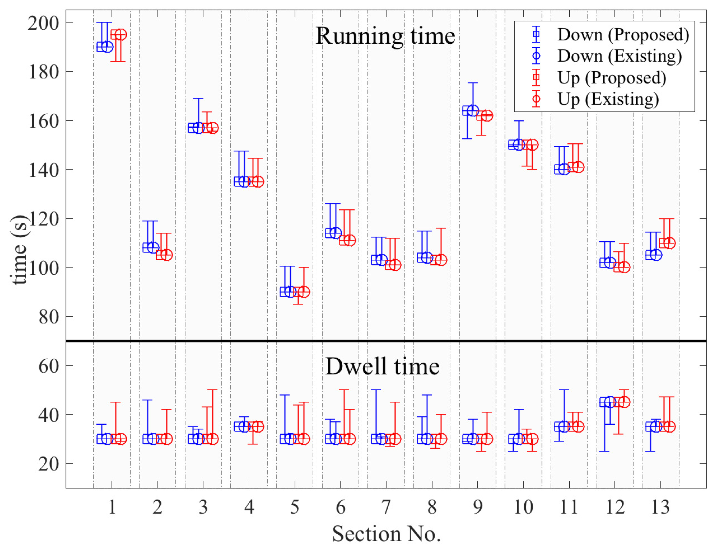
To analyze the impact of energy saving methods on the operation, the running time and the dwell time of the timetable and those of the energy saving methods with 300 s headway are illustrated in Figure 13.
The TEC/REC, the running/dwell time and the average traveling speed of short section scenarios with different headways are given in Table 2.
5.4. Discussion
5.4.1. Long Section Big Headway Scenario
It is shown in Figure 8 that the TEC of the proposed method is less than that of the existing method due to better utilization of regenerative energy. The TEC and REC data of 240 s headway at the end of simulation are presented in Table 1. It is concluded that both methods reduce TEC remarkably through making use of regenerative energy. Compared with the existing method, the proposed method can further reduce the tractive energy consumption by 8.5%.
Vectors are defined to represent the number of extended, unchanged and shortened running/ dwell time:
As shown in Figure 10, the and of the proposed method are and , respectively. Those of the existing method are and . It is observed that the proposed method extends the running time of most sections, shortens the dwell time of most stations to reduce the TEC. The existing method also extends the running time of most sections, and shortens about half of all the dwell time. The data of total running/dwell time and the average speed are presented in Table 1. The existing and the proposed methods have approximately the same average traveling speed as the timetable, which means that both methods have small impacts on operation. It should be noted that the proposed method is more energy efficient than the existing method and can realize an even higher average traveling speed than the timetable at the same time.
5.4.2. Long Section Small Headway Scenario
It is shown in Figure 9 that the proposed method is obviously more energy efficient since much more regenerative energy is used, when compared with the existing method. From the TEC and REC data of 90 s headway in Table 1, it can be found that, unlike the existing method, the proposed method is more energy efficient in a small headway. Based on the running time, dwell time and average traveling speed data, it can be concluded that the proposed method improves the utilization of regenerative energy through increasing the running time and decreasing the dwell time as in the case of big headway. Compared with the existing method, it can reduce the TEC by 19.1% and keep the average traveling speed not below that of the timetable simultaneously.
5.4.3. Short Section Big Headway Scenario
Comparing the TEC/REC curves in Figure 11 between the two energy saving methods, it can be found that the reduction in TEC is not as much as the increase in the REC of the proposed method. Since different speed profiles are selected by the two methods, although the TE of the proposed method is higher, much more regenerative energy is utilized to reduce the TEC by 8.4%, when compared with the existing method. It can be seen from Figure 13 that the and of the proposed methods are and , respectively. Those of the existing methods are and . Both methods increase the running time of most sections and the dwell time of most stations to improve the usage of regenerative energy. The average traveling speed of the two methods are close to that specified by the timetable, which means small impacts on the operation.
5.4.4. Short Section Small Headway Scenario
From the REC curves in Figure 12 and the data of the 90 s headway in Table 2, it is observed that both methods use much more regenerative energy in the short section small headway scenario than in other scenarios. The ratio of REC to TE of the proposed and the existing methods are and , respectively. The proposed method can save TEC by 14.9%. Both the running time and the dwell time are extended to improve the usage of regenerative energy, the difference in the average traveling speed between the proposed method and the timetable is larger than other scenarios. In general, the impacts of the two methods on the operation are small.
It can be concluded that the proposed method outperforms the existing method in every scenario. The improvement is remarkable, especially in a small headway. In long section scenarios, the proposed method can save energy and keep the average traveling speed not lower than that specified by the timetable. Its impact on the operation can be ignored.
6. Conclusions
In this paper, we proposed an improved train dispatch and control integrated energy saving method. We set up a ‘time slot and energy grid’ model, which can effectively reduce the complexity of analyzing the usage of regenerative energy among multiple bidirectional running trains. Based on the model, we designed the energy saving method. The running time of trains in sections, the dwell time of trains at stations and the headway (optional) were adjusted to synchronize the acceleration and deceleration of trains in the same electrical section, improve the utilization of regenerative energy and minimize the tractive energy consumption of all the trains on the line. To illustrate the effectiveness of the proposed method, the operational data of Beijing Changping and Beijing Yizhuang subway lines were used in simulation of long section and short section scenarios, respectively. When compared with an existing method, the proposed method can reduce the total tractive energy consumption by 8.5% and 19.1% in long sections big headway and long sections short headway scenarios, respectively. In the case of short section with big headway and small headway, the proposed method can save the total tractive energy consumption by 8.4% and 14.9%, respectively. It can be concluded that the proposed method has a significant improvement in energy saving in every scenario, especially in the case of a small headway. The remarkable performance is due to the improvement in the usage of regenerative energy. At the same time, the impacts of the proposed method on the operation of the urban rail transit were analyzed through comparison of the average traveling speed between timetable and the proposed method. Due to the constraints put on the adjustment of the running time and the dwell time, the impact of the proposed method on the operation can be ignored.
The method to calculate the energy saving was illustrated by simulation. It has not been validated by real data. We will take the parameters of the power network into consideration, study the on-line algorithm for rail-time traffic management and validate the energy saving effect of the method.
Author Contributions
All the authors contributed to the work of this paper. Bing Bu designed and developed the main parts of the research work, including the design of model and strategy, experimental and analyses of the simulation results. Guoying Qin contributed in simulation, experimental and writing parts. Ling Li and Guojie Li actively involved in verifying the work and finalize the manuscript. All authors have worked together on this paper and all authors have read and approved the final manuscript.
Acknowledgments
This research was funded by the Natural Science Foundation of Beijing Municipality grant number L61006 and 4164094, National Natural Science Foundation of China grant number 61603031, grant number RCS2017ZZ003, Innovation Fund of Beijing TCT grant number 9907006607 and Beijing Laboratory for Urban Mass Transit.
Conflicts of Interest
The authors declare no conflict of interest.
References
- Yang, X.; Li, X.; Ning, B.; Tang, T. A survey on energy-efficient train operation for urban rail transit. IEEE Trans. Intell. Transp. Syst. 2016, 17, 2–13. [Google Scholar] [CrossRef]
- Chen, J.; Cheng, S.; Nikic, V.; Song, M. Quo Vadis? Major Players in Global Coal Consumption and Emissions Reduction. Transf. Bus. Econ. 2018, 17, 112–132. [Google Scholar]
- González-Gil, A.; Palacin, R.; Batty, P.; Powell, J. A systems approach to reduce urban rail energy consumption. Energy Convers. Manag. 2014, 80, 509–524. [Google Scholar] [CrossRef]
- Takagi, R. Energy saving techniques for the power feeding network of electric railways. IEEJ Trans. Electr. Electron. Eng. 2010, 5, 312–316. [Google Scholar] [CrossRef]
- Kondo, K. Recent energy saving technologies on railway traction systems. IEEJ Trans. Electr. Electron. Eng. 2010, 5, 298–303. [Google Scholar] [CrossRef]
- González-Gil, A.; Palacin, R.; Batty, P. Sustainable urban rail systems: Strategies and technologies for optimal management of regenerative braking energy. Energy Convers. Manag. 2013, 75, 374–388. [Google Scholar] [CrossRef]
- Su, S.; Tang, T.; Chen, L.; Liu, B. Energy-efficient train control in urban rail transit systems. Proc. Ins. Mech. Eng. Part F 2015, 229, 446–454. [Google Scholar] [CrossRef]
- Wong, K.; Ho, T. Coast control of train movement with genetic algorithm. In Proceedings of the 2003 Congress on Evolutionary Computation, Canberra, Australia, 8–12 December 2003; Volume 2, pp. 1280–1287. [Google Scholar]
- Wong, K.K.; Ho, T.K. Dynamic coast control of train movement with genetic algorithm. Int. J. Syst. Sci. 2004, 35, 835–846. [Google Scholar] [CrossRef] [Green Version]
- Chang, C.; Sim, S. Optimising train movements through coast control using genetic algorithms. IEE Proc.-Electr. Power Appl. 1997, 144, 65–73. [Google Scholar] [CrossRef]
- Bocharnikov, Y.; Tobias, A.; Roberts, C.; Hillmansen, S.; Goodman, C. Optimal driving strategy for traction energy saving on DC suburban railways. IET Electr. Power Appl. 2007, 1, 675–682. [Google Scholar] [CrossRef]
- Yong, D.; Haidong, L.; Yun, B.; Fangming, Z. A two-level optimization model and algorithm for energy-efficient urban train operation. J. Transp. Syst. Eng. Inf. Technol. 2011, 11, 96–101. [Google Scholar]
- Tian, Z.; Hillmansen, S.; Roberts, C.; Weston, P.; Chen, L.; Zhao, N.; Su, S.; Xin, T. Modeling and simulation of DC rail traction systems for energy saving. In Proceedings of the 2014 IEEE 17th International Conference on Ntelligent Transportation Systems (ITSC), Qingdao, China, 8–11 October 2014; pp. 2354–2359. [Google Scholar]
- Milroy, I.P. Aspects of Automatic Train Control. Ph.D. Thesis, Loughborough University, Loughborough, UK, 1980. [Google Scholar]
- Howlett, P. The Optimal Control of a Train. Ann. Oper. Res. 2000, 98, 65–87. [Google Scholar] [CrossRef]
- Gong, C.; Zhang, S.; Zhang, F.; Jiang, J.; Wang, X. An integrated energy-efficient operation methodology for metro systems based on a real case of Shanghai metro line one. Energies 2014, 7, 7305–7329. [Google Scholar] [CrossRef]
- Yang, X.; Li, X.; Gao, Z.; Wang, H.; Tang, T. A cooperative scheduling model for timetable optimization in subway systems. IEEE Trans. Intell. Transp. Syst. 2013, 14, 438–447. [Google Scholar] [CrossRef]
- Yang, X.; Ning, B.; Li, X.; Tang, T. A two-objective timetable optimization model in subway systems. IEEE Trans. Intell. Transp. Syst. 2014, 15, 1913–1921. [Google Scholar] [CrossRef]
- Peña-Alcaraz, M.; Fernández, A.; Cucala, A.P.; Ramos, A.; Pecharromán, R.R. Optimal underground timetable design based on power flow for maximizing the use of regenerative-braking energy. Proc. Inst. Mech. Eng. Part F 2012, 226, 397–408. [Google Scholar] [CrossRef]
- Li, X.; Wang, D.; Li, K.; Gao, Z. A green train scheduling model and fuzzy multi-objective optimization algorithm. Appl. Math. Modell. 2013, 37, 2063–2073. [Google Scholar] [CrossRef]
- Albrecht, T. Reducing power peaks and energy consumption in rail transit systems by simultaneous train running time control. WIT Trans. State Art Sci. Eng. 2010, 39. [Google Scholar] [CrossRef]
- Nasri, A.; Moghadam, M.F.; Mokhtari, H. Timetable optimization for maximum usage of regenerative energy of braking in electrical railway systems. In Proceedings of the 2010 International Symposium on Power Electronics Electrical Drives Automation and Motion (SPEEDAM), Pisa, Italy, 14–16 June 2010; pp. 1218–1221. [Google Scholar]
- Bu, B.; Ding, Y.; Li, C.; Mao, X. Research on integration of train control and train scheduling. J. China Railw. Soc. 2013, 35, 64–71. [Google Scholar]
- Su, S.; Li, X.; Tang, T.; Gao, Z. A subway train timetable optimization approach based on energy-efficient operation strategy. IEEE Trans. Intell. Transp. Syst. 2013, 14, 883–893. [Google Scholar] [CrossRef]
- Su, S.; Tang, T.; Roberts, C. A Cooperative Train Control Model for Energy Saving. IEEE Trans. Intell. Transp. Syst. 2015, 16, 622–631. [Google Scholar] [CrossRef]
- Chen, E.; Yang, X.; Ding, Y. An energy-efficient adjustment approach in subway systems. In Proceedings of the IEEE International Conference on Intelligent Transportation Systems, Qingdao, China, 8–11 October 2014; pp. 2774–2779. [Google Scholar]
- Chen, E.; Bu, B.; Sun, W. An Energy-Efficient Operation Approach Based on the Utilization of Regenerative Braking Energy Among Trains. In Proceedings of the IEEE International Conference on Intelligent Transportation Systems, Las Palmas, Spain, 15–18 September 2015; pp. 2606–2611. [Google Scholar]
- Liu, W.; Li, Q.; Bing, T. Energy saving train control for urban railway train with multi-population genetic algorithm. In Proceedings of the 2009 International Forum on Information Technology and Applications, Chengdu, China, 15–17 May 2009; Volume 2, pp. 58–62. [Google Scholar]
- Liao, G.C. A novel evolutionary algorithm for dynamic economic dispatch with energy saving and emission reduction in power system integrated wind power. Energy 2011, 36, 1018–1029. [Google Scholar] [CrossRef]
- Alaca, F.; Sediq, A.B.; Yanikomeroglu, H. A genetic algorithm based cell switch-off scheme for energy saving in dense cell deployments. In Proceedings of the 2012 IEEE Globecom Workshops (GC Wkshps), Anaheim, CA, USA, 3–7 December 2012; pp. 63–68. [Google Scholar]
- Abramson, D.; Mills, G.; Perkins, S. Parallelisation of a genetic algorithm for the computation of efficient train schedules. Parallel Comput. Transp. 1994, 37, 139–149. [Google Scholar]
- Han, S.H.; Byen, Y.S.; Baek, J.H.; An, T.K.; Lee, S.G.; Park, H.J. An optimal automatic train operation (ATO) control using genetic algorithms (GA). In Proceedings of the 1999 IEEE Region 10 Conference, Cheju Island, Korea, 15–17 September 1999; Volume 1, pp. 360–362. [Google Scholar]
- Li, Y.; Hou, Z. Study on energy-saving control for train based on genetic algorithm. J. Syst. Simul. 2007, 2, 38. [Google Scholar]
- Chung, J.W.; Oh, S.M.; Choi, I.C. A hybrid genetic algorithm for train sequencing in the Korean railway. Omega 2009, 37, 555–565. [Google Scholar] [CrossRef]
- Zhang, Y.S.; Jin, W.D. Model and algorithm for train operation adjustment on single-track railways based on genetic algorithm. J. Southwest Jiaotong Univ. 2005, 40, 147–152. [Google Scholar]
Figure 1.
Synchronizing the deceleration and acceleration of trains.

Figure 2.
The “two-time traction” control strategy.

Figure 3.
Multiple bidirectional running trains in different electrical sections.
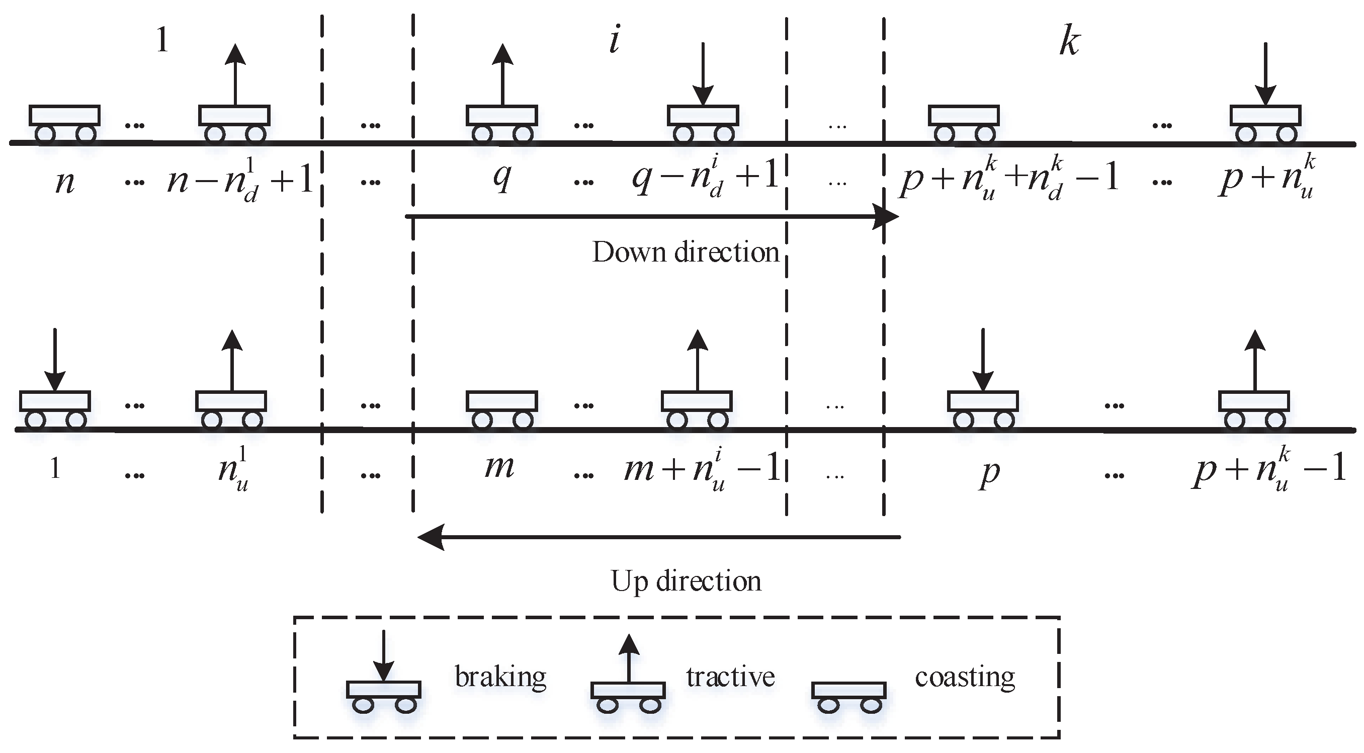
Figure 4.
A schematic diagram of the time slot and energy grid model.

Figure 5.
The schematic diagram of a typical subway line.
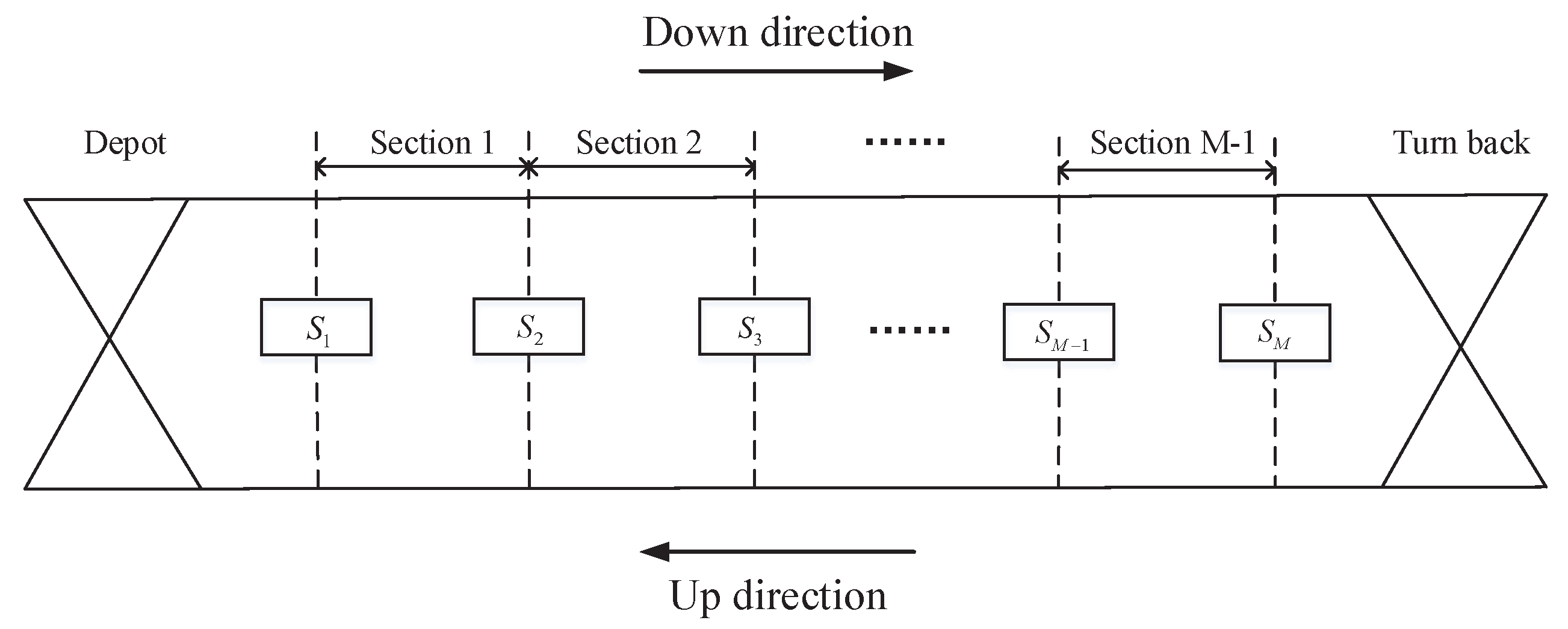
Figure 6.
Speed profiles of the first section of BJCP in the down direction.

Figure 7.
The best and the mean penalty value of GA (Changping, = 240 s).

Figure 8.
Energy consumption of the energy saving methods (BJCP, = 240 s).
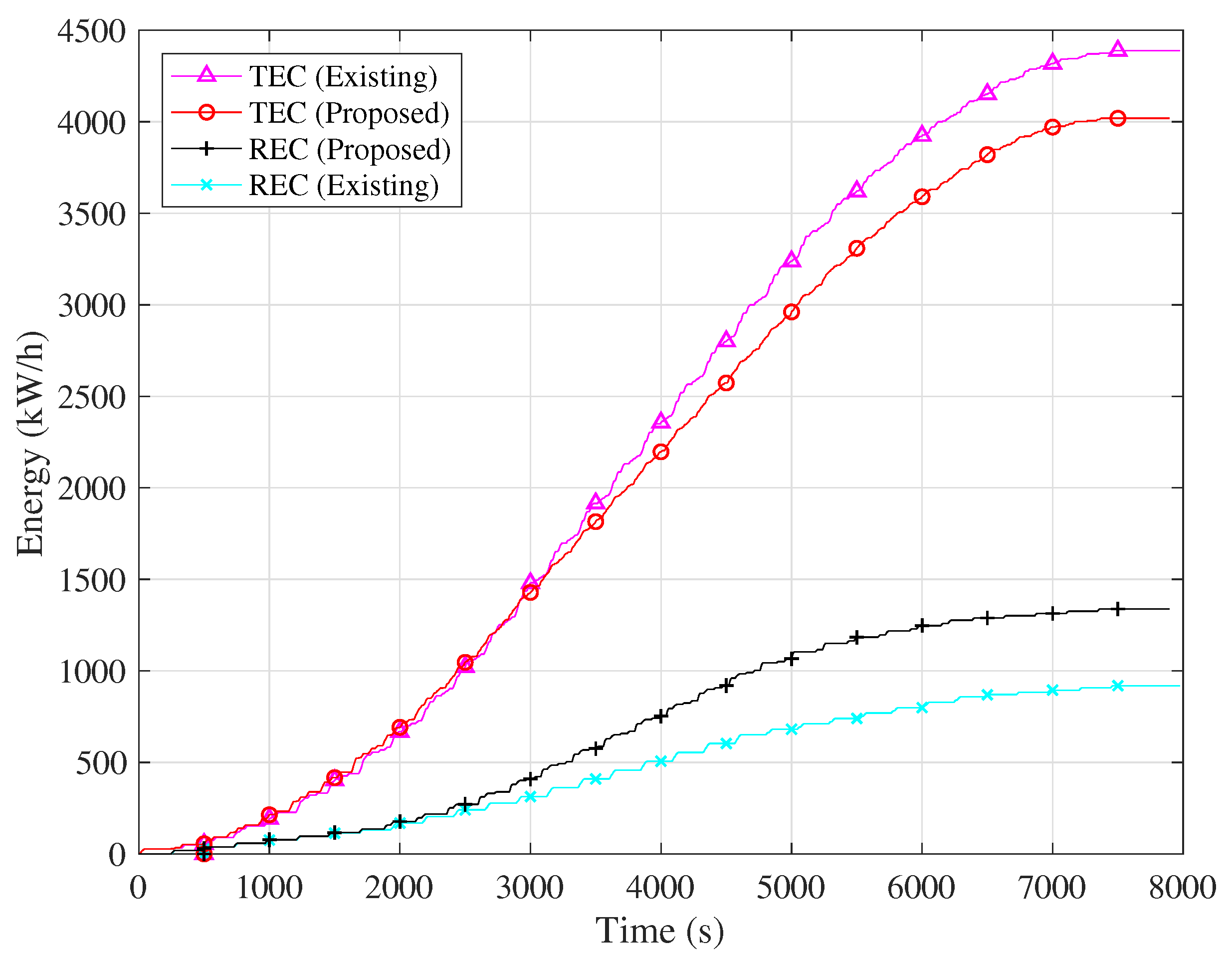
Figure 9.
Energy consumption of the energy saving methods (BJCP, = 90 s).

Figure 10.
Comparison of the running/dwell time between the timetable and the energy saving methods. (BJCP, = 240 s).
Figure 10.
Comparison of the running/dwell time between the timetable and the energy saving methods. (BJCP, = 240 s).
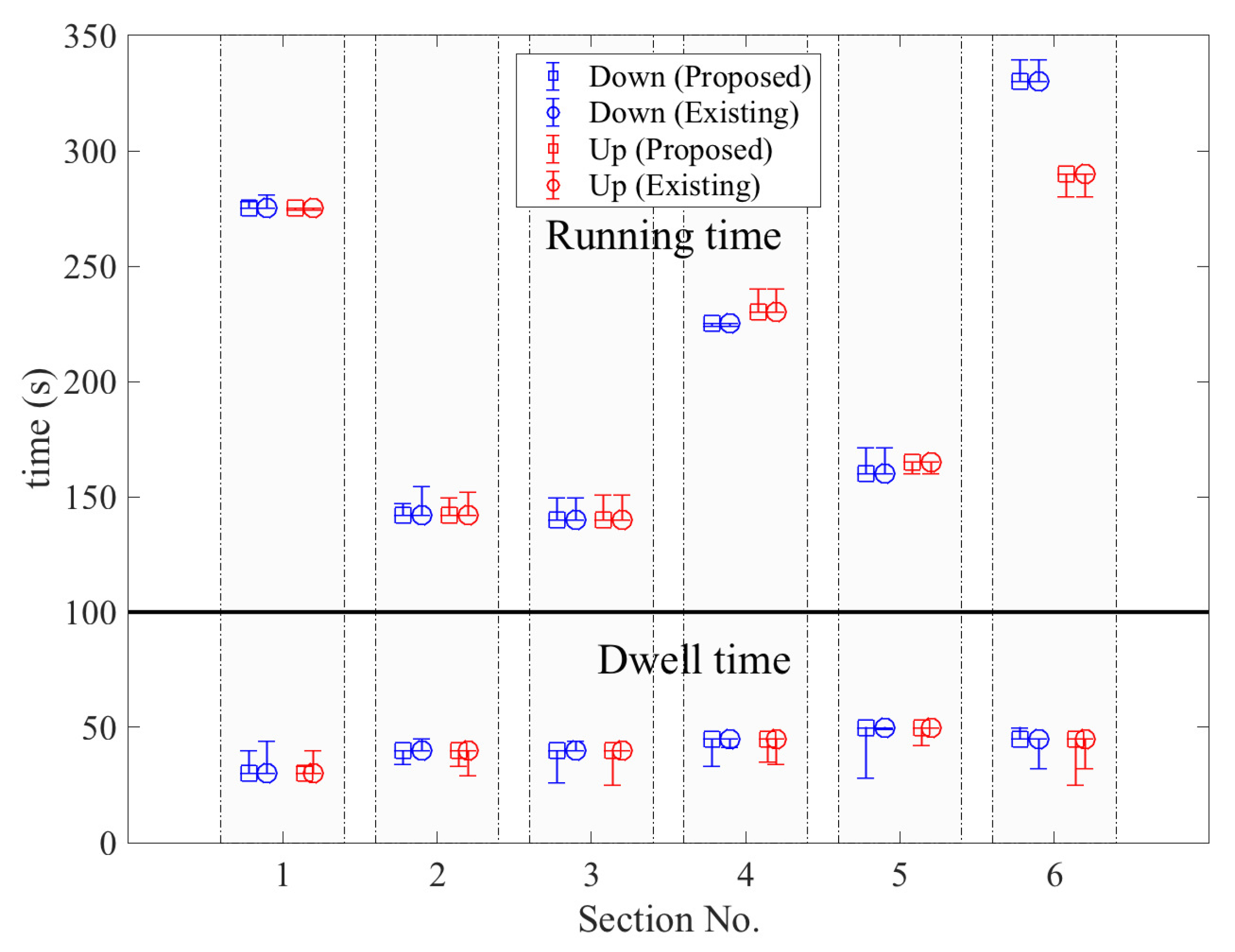
Figure 11.
Energy consumption of the energy saving methods (BJYZ, = 300 s).
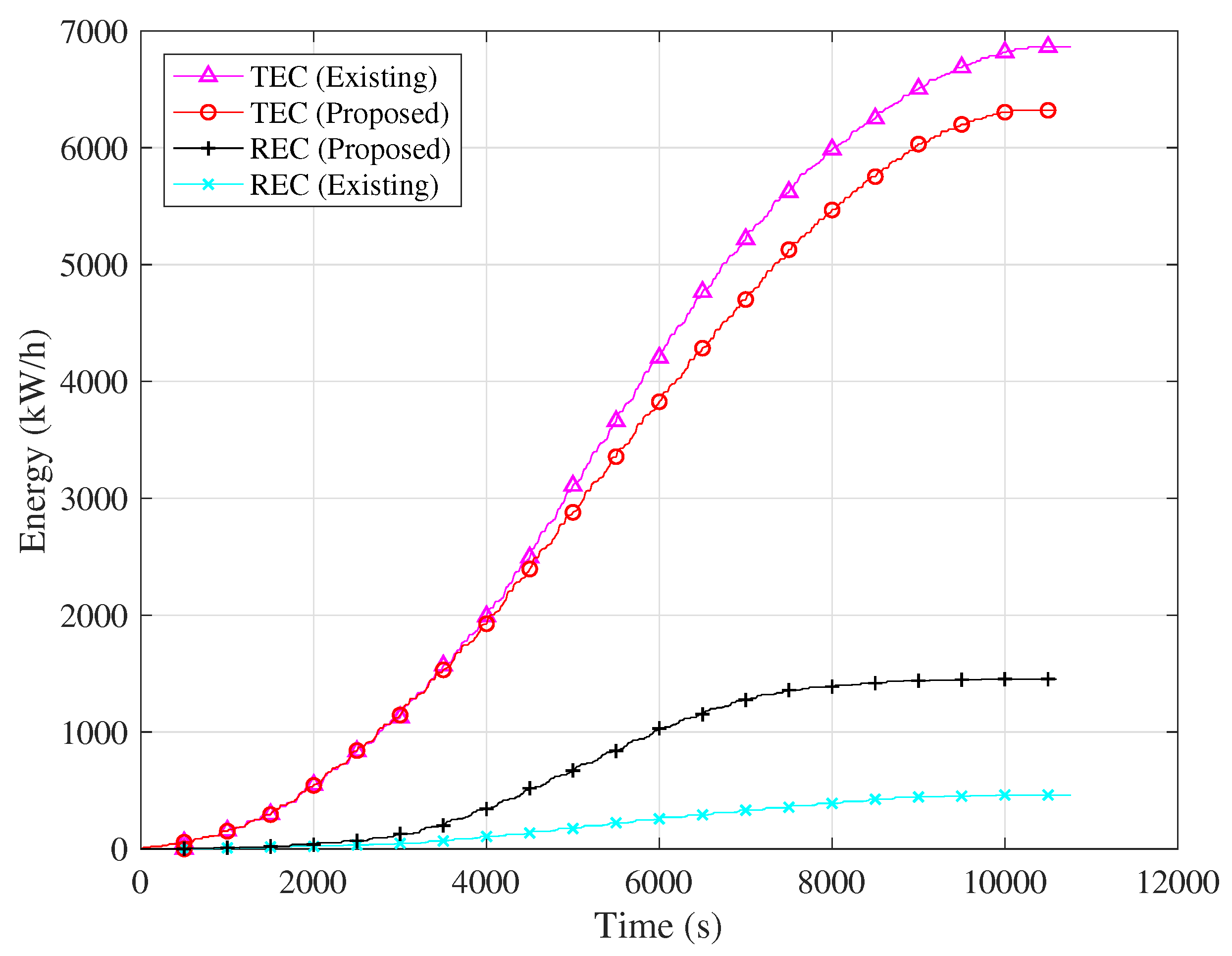
Figure 12.
Energy consumption of the energy saving methods (BJYZ, = 90 s).

Figure 13.
Comparison of the running/dwell time between the timetable and the energy saving methods. (BJYZ, = 300 s).
Figure 13.
Comparison of the running/dwell time between the timetable and the energy saving methods. (BJYZ, = 300 s).


Table 1.
The energy consumption, running/dwell time and average traveling speed of the energy saving methods (BJCP)
Table 1.
The energy consumption, running/dwell time and average traveling speed of the energy saving methods (BJCP)
| Headway | Methods | TEC (kWh) | REC (kWh) | Run time (s) | Dwell time (s) | (km/h) |
|---|---|---|---|---|---|---|
| 240 s | Timetable | 5616.3 | 0 | 2514 | 500 | 44.52 |
| Existing | 4388.8 | 919.1 | 2576.6 | 474 | 44.05 | |
| Proposed | 4015.7 | 1348.4 | 2563.5 | 404 | 45.13 | |
| 90 s | Existing | 4740.9 | 629 | 2571.5 | 453 | 44.38 |
| Proposed | 3835.5 | 1700.3 | 2531.5 | 476 | 44.61 |
Table 2.
The energy consumption, running/dwell time and average traveling speed of the energy saving methods (BJYZ).
Table 2.
The energy consumption, running/dwell time and average traveling speed of the energy saving methods (BJYZ).
| Headway | Methods | TEC (kWh) | REC (kWh) | Run Time (s) | Dwell Time (s) | (km/h) |
|---|---|---|---|---|---|---|
| 300 s | Timetable | 8578.4 | 0 | 3322 | 840 | 35.98 |
| Existing | 6862.3 | 461 | 3532 | 1019 | 33.15 | |
| Proposed | 6284.2 | 1444.9 | 3454.5 | 932 | 34.29 | |
| 90 s | Existing | 5027.8 | 2895.4 | 3430 | 1007 | 33.93 |
| Proposed | 4281.3 | 3789.7 | 3420.5 | 1026 | 33.86 |
© 2018 by the authors. Licensee MDPI, Basel, Switzerland. This article is an open access article distributed under the terms and conditions of the Creative Commons Attribution (CC BY) license (http://creativecommons.org/licenses/by/4.0/).
Share and Cite
MDPI and ACS Style
Bu, B.; Qin, G.; Li, L.; Li, G. An Energy Efficient Train Dispatch and Control Integrated Method in Urban Rail Transit. Energies 2018, 11, 1248. https://doi.org/10.3390/en11051248
AMA Style
Bu B, Qin G, Li L, Li G. An Energy Efficient Train Dispatch and Control Integrated Method in Urban Rail Transit. Energies. 2018; 11(5):1248. https://doi.org/10.3390/en11051248
Chicago/Turabian StyleBu, Bing, Guoying Qin, Ling Li, and Guojie Li. 2018. "An Energy Efficient Train Dispatch and Control Integrated Method in Urban Rail Transit" Energies 11, no. 5: 1248. https://doi.org/10.3390/en11051248
Note that from the first issue of 2016, this journal uses article numbers instead of page numbers. See further details here.