Advances in Pore-Scale Simulation of Oil Reservoirs

Abstract

At the high water cut stage, the residual oil in a reservoir becomes complex and dispersed. Moreover, it is challenging to achieve good predictions of the movement of oil and water in a reservoir according to the macroscopic models based on the statistic parameters of this scenario. However, pore-scale simulation technology based on directly tracking the interaction among different phases can make an accurate prediction of the fluid distribution in the pore space, which is highly important in the improvement of the recovery rate. In this work, pore-scale simulation methods, including the pore network model, lattice Boltzmann method, Navier–Stokes equation-based interface tracking methods, and smoothed particle hydrodynamics, and relevant technologies are summarized. The principles, advantages, and disadvantages, as well as the degree of difficulty in the implementation are analyzed and compared. Problems in the current simulation technologies, micro sub-models, and applications in physicochemical percolation are also discussed. Finally, potential developments and prospects in this field are summarized.

1. Introduction

At the high water cut or super high water cut stages in oilfields, residual oil distribution becomes complex and dispersed. Thus, it becomes more difficult to take in-depth measures in order to improve the recovery rate. At this stage, the movement of oil and water is controlled by rock wettability, pore structure characteristics, physical property of the fluid, and mining scheme. Oil–water movement at the pore-scale directly determines the displacement efficiency in an oil reservoir. Further study of the movement characteristics of oil and water at the pore-scale as well as the effects of control factors (rock wettability, pore structure characteristics, physical property of the fluid, and development plan) is essentially important to further enhance the oil recovery at the high water cut stage. However, most of the studies on the movement of oil and water phases at the pore-scale are limited to physical experiments because of the complicated pore structure in oil reservoirs [1]. As an important research method, numerical simulation technology is extensively used in macroscopic oil reservoirs, but rarely used at the microscopic pore-scale. With the development of oil reservoir simulation technology, pore-scale simulation technology for oil reservoirs has gradually become an important means to study multi-phase fluid interaction, microscopic residual oil formation mechanics, and oil distribution in pore space.

The movement of oil and water at the pore-scale determines the spatial distribution of residual oil. The multi-phase movement in porous media in an oil reservoir is mainly affected by the fluid property, pore structure, and mining scheme. Complicated physical and chemical changes as well as heat and mass transfer in the pore space can change the rheological property or phase interaction strength. Meanwhile, fluid flow process also affects the physical and chemical changes and heat and mass transfer behaviors. Under high pressure, the pore structure also may deform and even rupture. Compared with the macroscopic movement of a multi-phase fluid in porous media, the main control factor of a multi-phase fluid flow at the pore-scale has changed. Interfacial tension plays a more and more important role, and sometimes it dominates the flow process. Interfacial tension is controlled by the size of a pore, chemical composition in the two-phase fluid. Meanwhile, the wetting film that builds up due to pore wall micro-roughness affects the wettability of the oil/water/porous medium system by changing the dynamic contact angles of the o/w menisci [2]. Construction of a basic mathematical model describing multiphase flow in pore space and sub-models describing the effect of micro-physical-chemical process on the multiphase flow dynamics is essentially important for accurate prediction of the pore-scale oil–water behaviors. However, research on the method of pore-scale simulations in oil reservoirs started relatively late. Apart from the pore network model, other methods are limited to the study of the flow process with constant model parameters. Micro sub-models, such as the film model, micro-roughness model, or non-Newton effect of the oil phase, etc. are generally not included. Thus, these models are very far from engineering applications.

In this work, the pore-scale simulation methods and relevant technologies are summarized. The principles, advantages, and disadvantages, as well as the degree of difficulty in the implementation of the pore network model (PNM), lattice Boltzmann method (LBM), Navier–Stokes equation based interface capturing methods (NS), and smoothed particle hydrodynamics (SPH) are analyzed and compared. Problems in the current simulation technologies, micro sub-models, and applications in physicochemical percolation are also discussed. Finally, potential developments and prospects in this field are addressed.

2. Pore-Scale Simulation Method for Oil Reservoirs

In order to give an overview of the methods discussed in this work, we present a comparison in terms of the framework used, parallel treatment difficulty, model accuracy, computational loads, linear system included, implementation difficulty, and pore-scale modeling maturity in

Table 1. Comparisons among different pore-scale simulation methods.

Method	Framework	Parallel	Model Accuracy	Computational Loads	Linear System	Implementation	Pore-Scale Modeling Maturity
PNM	Euler	Difficult	Low	Low	Yes	Easy	Mature
LBM	Euler	Easy	High	High	No	Easy	Immature
NS	Euler	Difficult	High	High	Yes	Difficult	Immature
SPH	Lagrange	Easy	High	Very High	Yes/No	Easy	Immature

. One should choose the appropriate method according to the specific application.

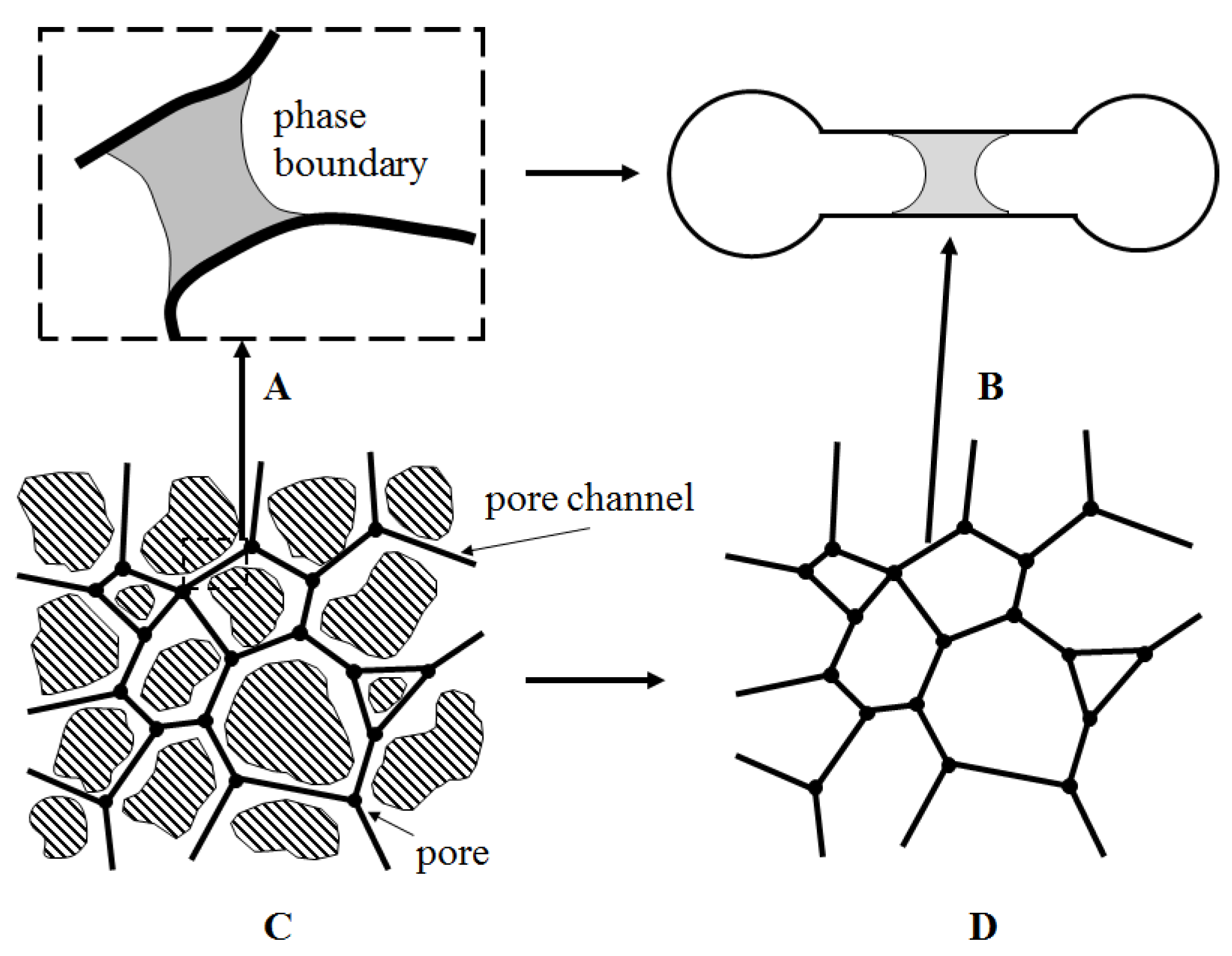
2.1. Pore Network Model

The pore network model is one of the earliest models used for pore-scale simulation. In this model, complicated pore space is simplified as pores and channels (or throats) connecting pores. The throat is usually approximated as regular shapes, such as column, triangular prism, or square column, etc. Such a network consisting of pores and throats is referred to as a pore network. The pore network can be created by the random structuring method or the digital core method [3]. A pore network created by the random structuring method contains pores conforming to specific statistical laws [4,5,6]. The model parameters for the pore network reconstructed from a digital core are directly from real pore space approximation [7,8,9]. A sketch of the reconstructed pore network from real pore space (given in Figure 1C) is given in Figure 1D. The points in this figure denote pores. For a specific channel, the possible fluid distribution is shown in Figure 1A. However, the physical model adopts the simplified figure shown in Figure 1B in modeling process.

The pore network model creates a pore node equation by the pore throat connectivity in order to obtain the state of each node. For example, the two-phase pore network model with piston-like displacement assumption creates the relationship between the adjacent nodes by the following equation:

$$Q_{ij}=G_{ij}\left(p_i-p_j-\Delta p_{ij}^c\right)$$

(1)

where Q_ij is the channel flow rate between two adjacent nodes; p_i and p_j denote the pressure at node i and node j, respectively; G_ij is a variable related to throat geometry and fluid viscosity. $\Delta p_{ij}^c$ is the capillary pressure jump across the fluid-fluid interface in the channel connecting node i and node j. In general, the capillary pressure jumps across a fluid–fluid interface is given by Yong–Laplace Equation

$$p_c=\sigma \left(\frac{1}{R_1}+\frac{1}{R_2}\right)$$

(2)

where, σ is surface tension, R₁ and R₂ are the principal radii of curvature. In simulating flow in the network, modified equation for the local capillary pressure is also used, for instance, Aker et al. using the following equation [10]

$$p_c=\frac{2\sigma }{r}\left(1-\cos \left(2\pi x\right)\right)$$

(3)

where x represents the position of the interface within the throat, i.e., 0 ≤ x ≤ 1. If there are several interfaces in a single throat, the capillary pressure between the node i and node j is given by (4)

$$\Delta p_{ij}^c={\displaystyle {\sum }_k^n{p}_{ck}}$$

(4)

n is the total number of the interfaces in the throat.

It should be stressed that Equation (3) is a phenomenological model with the assumption that capillary force is zero at two ends and largest at the center of the capillary tube. This is relatively more accurate than the model with the assumption the capillary tube being uniform. However, if the radius along the capillary tube is known, the capillary force can be calculated accurately using the Yong–Laplace Equation. However, the pore-network extraction from a real pore space can be complex.

In addition to the general equations requiring the simulating dynamics of two-phase flow in a pore network models, some local rules should be defined as well. For instance, entry capillary pressure rule [11], snap off rule [12]. Flow regimes models are also possible to join, for instance, film dynamics [13] and ganglion dynamics [14].

Depending on the flowing conditions within a channel, the impact of capillary force and viscous force on the flow behaviors and distribution of the disconnected oil elements can be different. Macroscopic flow can be decomposed into two prototype flows: The connected oil pathway flow (CPF) and the disconnected oil flow (DOF). The latter can be further decomposed into ganglion dynamics (GD) flow and drop traffic flow (DTF) [15]. If the interstitial velocity is large enough, the viscous force dominates the fluid flow. The connected oil pathway can be fragmented, following which a disconnected oil flow pattern forms. Depending on the local interstitial velocity, the ganglia can move through several pores simultaneously or separate further to form drops. The drops or ganglia can also become stranded in local pores if the interstitial velocity is relatively small and the interfacial tension dominates the fluid behavior. The ganglia or drops can also coalescence to form large ganglia or drops.

The capillary number Ca, representing the relative importance of viscous force and capillary force, is defined as:

$$Ca=\frac{\rho vU}{\sigma }$$

(5)

where ρ, v, and U are the density, kinematic viscosity, and velocity of the fluid. σ is the interfacial tension coefficient. With the increase of Ca, the break-up probability of ganglia or drops also increases. For instance, during the flow process of drops in porous media, Zinchenko, A.Z. et al. found that drop breakups are still not observed for Ca = 0.009 and that only rare, isolated breakups are encountered for Ca = 0.012–0.015. In contrast, for Ca = 0.02, the emulsion drops are prone to frequent fragmentation [16]. Incorporating the different flow regimes into pore network models to achieve an accurate prediction of flow behaviors is a difficult task that should be further investigated in depth, although considerable efforts have been devoted to this issue [14,17,18,19,20].

According to the conservation of flow, the flow rate at any node i meets the following equation:

$$Q_i={\displaystyle \sum {}_j}{Q}_{ij}$$

(6)

where j is the node index of the node connected to node i. If the boundary pressure is specified, the boundary nodes meet the following equation:

$$p_i=p_{bi}$$

(7)

where p_bi is the pressure at the ith boundary node. The flow rates of the channels connected to this node are evaluated by Equation (1) and the total flow rate at this node is evaluated by Equation (6), accordingly. If the boundary flow rate is specified, the following equation is met:

$${\displaystyle {\sum }_i{Q}_{ij}=-F_{bi}}$$

(8)

where F_bi is the total flow rate across the ith boundary node.

An equation set consisting of all of the node pressures in the system can be obtained by a combination of Equations (1), (6)–(8). After solving, the pressure at each node can be obtained, and the flow rate of each connecting channel can be obtained from Equation (1). Finally, the two-phase interface location and the volume of each phase in each pore can be calculated from the flow rate.

The piston-like displacement assumption only applies to a certain flow pattern. However, there are usually many flow patterns in the actual displacement scenario in an oil reservoir. Thus, it is necessary to develop more complicated models to improve the prediction accuracy. More complicated physical and chemical processes, such as the mass transfer process [21,22,23,24,25,26,27], biological process [28], and foam displacement [29,30], etc., have been taken into account in the pore network model [4,31,32,33,34,35]. For details about the pore network model, see References [36,37].

The pore network model was developed earlier, and is very mature for single-phase flow and two-phase flow and has been expanded to a three-dimensional (3D) three-phase model by considering the complicated physical and chemical processes involved [38,39,40,41]. With the development of computer graphics, the pore network can be structured by real core images, bridging the gap of the pore network structure and the real core structure. This model requires a smaller computational expense and works more easily than other pore-scale simulation technologies. However, the presence of the pore geometry assumption and physical process assumption leads to difficulty in evaluating the exact fluid dynamic topology structure in actual pore channels, and makes it impossible to study the flow behaviors caused by a velocity difference in the pore channel cross-section (for instance, phase distribution in the cross-section). Therefore, this model has a lower prediction accuracy of residual oil distribution than other models. However, this model is so mature and simple that it continues to play an important role in the pore-scale simulation of oil reservoirs. A systematic and extensive review of pore network models can be found in the work of V. Joekar Niasar and S.M. Hassanizadeh [42].

2.2. Lattice Boltzmann Method

The lattice Boltzmann method is a fluid flow simulation method that has been developed very quickly over recent years and is not based on the continuity assumption [43,44]. This method does not directly track macroscopic quantity but the number density function of velocity. The macroscopic flow state can also be obtained accordingly based on the number density function. This method first discretizes the velocity space in the continuous Boltzmann equation to obtain the discrete Boltzmann equation, and then discretizes the time and location in the discrete Boltzmann equation to obtain the lattice Boltzmann equation. Finally, it achieves the solution of the lattice Boltzmann equation by simple operations of “migration” and “collision”. Equation (9) gives the continuous Boltzmann–Bhatnagar–Gross–Krook (Boltzmann BGK) equation [45]:

$$\frac{\partial f}{\partial t}+\mathsf{\xi }\cdot \nabla f=\frac{1}{{\tau }_c}\left[f-f^{eq}\right]$$

(9)

where f is the number density distribution function of velocity, τ_c is the relaxation time, and f^eq is the Maxwell equilibrium distribution. Taylor expansion is conducted for the equilibrium distribution function in velocity space, and the moment of the equilibrium distribution function is calculated from the Gaussian integral formula in order to ensure that the number density function, f, has a discrete moment equal to continuous moment. Finally, the resultant discrete Boltzmann equation is discretized along characteristic line, and the following equation is obtained:

$$f_i(\mathbf{x}+{\mathbf{c}}_i{\delta }_t,t+{\delta }_t)-f_i(\mathbf{x},t)=\frac{1}{\tau }[f_i(\mathbf{x},t)-f_i^{eq}(\mathbf{x},t)]$$

(10)

where c_i is the characteristic velocity and δ_t is the lattice time step. τ is the dimensionless relaxation time, expressed by τ_c/δ_t. The solution of the above equation can be obtained by dealing with “collision” after “migration” operations. Finally, macroscopic quantities, such as density, pressure, and velocity, can be easily obtained. Multi-phases/multi-components usually coexist in the pores in oil reservoirs. Therefore, the lattice Boltzmann method creates a model similar to Equation (10) for each phase. The interfacial tension between two phases can be expressed by the Shan/Chen model [46,47]:

$$F_i(\mathbf{x},t)=-\psi (\mathbf{x},t){\displaystyle {\sum }_{k=1}^N{\displaystyle {\sum }_i{G}_{jk}(\left|{\mathbf{c}}_i\right|)}}{\psi }_k\left(x+{\mathbf{c}}_{i}t\right){\mathbf{c}}_i$$

(11)

where ψ(x, t) is the density function and G_jk is the interaction strength. This equation can also be used for the interactions between the fluid and solid walls.

The study on multi-phase flow simulation by the lattice Boltzmann equation mainly focuses on three aspects: (a) The implementation of interfacial tension and the treatment of wall wettability; (b) the elimination of velocity spurious currents near the phase interface; and (c) the implementation of a high viscosity ratio or a high-density ratio model. For example, He et al. did not distinguish between dynamic pressure and static pressure in the double distribution function two-phase flow simulation method developed by them. This method can reduce spurious currents on the interface, but cannot eliminate the phase interface spurious currents [48]. Shiladitya et al. introduced an external force model to this method in order to deal with the wall wettability [49]. Lee et al. developed a two-phase flow model to process the high viscosity ratio or density ratio up to 1000, as well as to suppress the spurious currents on the interface [50].

The lattice Boltzmann method has been used in pore-scale simulations [51,52,53,54,55,56], but mostly for methodology research and rarely for flow simulations in real pore geometry in an oil reservoir. The lattice Boltzmann method develops very quickly in pore-scale simulation of porous media for its easy treatment of complex boundary. As shown in Figure 2, the lattice Boltzmann method is used to describe the porous media zone shown in Figure 1C (it must be pointed out that this figure is only a schematic, so the lattice used in the actual simulation is denser than that shown in Figure 2). The quadrate mesh in this figure depicts the lattice used in the lattice Boltzmann method (this method must use square Cartesian mesh with the same dimensions because of its own features). In a pore-scale porous media simulation, the lattice Boltzmann method involved the classification of lattice sites according to their locations. For example, A is in the solid zone in Figure 2, and is marked as 1, while B is in the fluid zone, and is marked as 0. The classification of lattice sites usually can be set according to the gray-scale value in CT (computed tomography) scanning images of the porous media. The “bound-back” boundary condition is easily used for the processing of the particle migration between a fluid node (such as Node B) and a solid node (such as Node C). However, a standard “bound-back” boundary condition is only of the first order in accuracy, so a special curve boundary processing method is usually used for complicated structures [57] or local refinement is performed to ensure that the mesh is able to meet engineering requirements. If the curve boundary processing method is used, the intersection points between the lattices and pore surface need to be calculated. At this time, reconstruction of the pore structure is needed, resulting in many difficulties and the loss of advantages of “bound-back” scheme. Local refinement automatically according to local pore structure is also a tough task. Generally, the mesh arrangement based on the size of the smallest throat leads to a denser mesh arrangement in big pores, resulting in a sharp increase in computational expense, especially for a porous structure with a large pore-throat ratio. In this case, it is very difficult to achieve the flow simulation at a larger scale.

The lattice Boltzmann method has the following advantages: (a) It is easy to implement, unnecessary to solve linear system, easy in parallelization processing; (b) it is able to directly process the complicated geometry by “bound-back” scheme, which is essentially advantageous to process the flow in porous media; (c) with LBM, pore-scale simulation can be carried out with micro-computed-tomography images of the porous media [58,59], and mesh is unnecessary. For instance, Ramstad T, et al. used the lattice Boltzmann method to simulate the two-phase flow directly on the digital images of porous rocks and compute the relative permeability [60]. On the other side, this method has some disadvantages: (a) It requires a large computational expense and parallel processing is needed for large-scale simulation; (b) it exhibits low stability of the available multi-phase flow model when processing a high-density ratio, high viscosity ratio, or low Schmidt number multi-component flow; (c) it is necessary to refine the mesh or use the curve boundary processing method in order to enhance the accuracy of the method because the “bound-back” scheme is of first-order accuracy; (d) it actually requires a low Mach number of the flow, but does not apply to a high macroscopic percolation rate of the flow at the pore-scale (such as the flow near the well bore) [43]; and (e) for a non-isothermal flow, the lattice Boltzmann method becomes relatively complicated.

2.3. Navier–Stokes Equation-Based Interface Capturing Method

The Navier–Stokes equation is widely used in macroscopic flow. The pore-scale adaptability of this equation can be calculated from the pore Knudsen number, Kn, which is defined as:

$$Kn=\frac{\lambda }{L}$$

(12)

where λ is the mean free path of the fluid and L is the characteristic length of the geometry specifically, the throat radius is used in the pore-scale flow. At Kn ≤ 0.001, the fluid is in the continuous zone, so Navier–Stokes is extensively used. At 0.001 < Kn ≤ 0.1, the fluid is in the slip zone, so the continuity assumption will not be satisfied, but Navier–Stokes and slip boundary conditions can still be used to describe the physical problems in this zone. At Kn > 0.1, Naiver–Stokes will never apply [43]. This is the general description of the microscale flow adaptability of the Navier–Stokes equation.

Weng, H.C. et al. proved through experiments and simulation research that maximum Kn for Navier–Stokes and second-order Maxwell-Burnett slip boundary is 1.6 [61]. At atmospheric temperature and pressure, the mean free path of air is about 8 × 10⁻⁸ m. From Equation (12), we can get that the Navier–Stokes equation can be used for pores with a throat radius of more than 50 nm. However, the throat radius in low permeability oil reservoirs is more than this value [62]. Under the actual conditions of oil reservoirs, the combination of recovery pressure and formation pressure leads to the pressure in the real pores in oil reservoirs being much higher than the atmospheric pressure, resulting in a theoretical mean free path of gas in the pores that is much lower than the mean free path at atmospheric temperature and atmospheric pressure, and further increase the adaptability of the Navier–Stokes Equation in pore-scale simulation of oil recovery. Liquids have a much lower mean free path than gases, so any situations suitable for gases are suitable for liquids. Thus, the macroscopic Navier–Stokes equation completely adapts to the pore-scale simulation of oil recovery.

To apply the macroscopic Navier–Stokes equation based interface capturing method to the actual pore-scale simulation of an oil reservoir, it is necessary to mesh the pore geometry firstly. However, due to complex characteristics of pore geometry, the pore meshing process should be carried out by CutCell [63] or Delaunay triangulation [64] technology automatically. The free surface can be captured by the Level Set [65] or VOF (volume of fluid) method [66]. The Level Set method can obtain a two-phase interface with high accuracy but cannot guarantee the conservation of the tracked fluid. The equations in VOF based two-phase immiscible flow modeling technology are [67]:

Continuity equation

$$\nabla \cdot \mathbf{u}=0$$

(13)

Momentum equation

$$\frac{\partial \rho \mathbf{u}}{\partial t}+\nabla \cdot \left(\rho \mathbf{uu}\right)-\nabla \cdot \left(\mu \mathbf{S}\right)=-\nabla p+\rho \mathbf{g}+\sigma K\mathbf{n}$$

(14)

Volume fraction equation

$$\frac{\partial \rho \alpha }{\partial t}+\nabla \cdot \left(\rho \mathbf{u}\alpha \right)=0$$

(15)

where u is the volume average velocity of the multi-phase fluid, S is the strain rate tensor expressed as (∇u + ∇u^T), σ is the interfacial tension coefficient between two phases, α is the phase volume fraction, K is the interface curvature expressed as ∇∙(∇α/|∇α|), and n is the normal direction of the interface expressed as ∇α/|∇α|. Equations (13)–(15) still adapt to the fluid flow in pores in oil reservoirs, and can be discretized and solved by standard discrete methods such as the finite volume method, finite element method, etc.

Different from the traditional macroscopic free interface flow, the interfacial tension between two phases can dominate pore-scale two-phase behaviors. Generally, the capillary number Ca can be used to characterize the viscosity force and interfacial tension. In the actual pore-scale flow in an oil reservoir, Ca is typically between 10⁻¹⁰ and 10⁻⁵. Thus, treating interfacial tension with high accuracy is essentially important for pore-scale two-phase flow behaviors prediction.

Under the Euler framework, the interfacial tension implementation methods include the continuous interface stress method [68], continuous interface force method (CSF) [69], sharp surface force method [70], and ghost fluid method [71]. However, these methods unavoidably have a spurious currents problem on the interface between two phases at a high interfacial tension caused by the imbalance between surface tension and pressure gradient at the surface. This spurious velocity can be expressed by the following equation [68]:

$$u_{s,\max }=K\frac{\sigma }{\mu }$$

(16)

where K is a constant at the order of magnitude of 10⁻², denoting the strength of the spurious currents. This equation describes the dependence of the spurious currents on the fluid property. It is just employed to estimate the spurious currents. The concrete value depends on accuracy for evaluating the interfacial tension. If the spurious velocity is larger than the physical flow velocity in pores of the oil reservoir, the prediction accuracy of traditional VOF methods is limited. Raeini, A.Q. used a simple filtration method to eliminate spurious velocity [70]. In the meanwhile, they conduct a simulation of the digital core using VOF method, and bridge the gap between the numerical predicted behaviors and macroscopic parameters [72], and reproduces some exclusive phenomena at the pore-scale in the oil reservoir [73]. How to eliminate spurious currents at high interfacial tension is still a subject of major concern in VOF simulation.

The VOF method has the following advantages: (a) It employs the Navier–Stokes equation to directly calculate the pore-scale flow process without any geometric approximation, really reflects the actual flow in the pores, and possesses high calculation accuracy; (b) only three equations are needed and local mesh refinement can be easily carried out with this method. Thus, the computational load is much less than lattice Boltzmann method; (c) VOF model can be used to describe multi-phase flow and is very mature, not restricted by multi-phase fluid properties (such as density, etc.), and suitable for any two-phase or three-phase flow simulation; (d) as a traditional method, this method is more easily used in physicochemical percolation. However, the VOF method also presents some disadvantages: it is necessary to reconstruct the pore geometry from actual porous media (such as digital core) and mesh the pore space, resulting in an increased workload at the early stage of the simulation.

2.4. Smoothed Particle Hydrodynamics

In addition to the above three methods, smoothed particle hydrodynamics [74,75,76] is another widely used numerical method for multi-phase flow in porous media [77]. As a mesh-less method, the smoothed particle hydrodynamics method uses the discrete technique in the particle method to solve the Navier–Stokes equation and guarantee multi-phase interface sharpness without the tracking of the two-phase or multi-phase interface. For a given fluid particle, the equation of motion is given by [75,78]:

$$\begin{array}{ll}\frac{d{\mathbf{u}}_i}{dt}=& -{\displaystyle \sum {}_j}{m}_j\left(\frac{p_i}{{\rho }_i^2}+\frac{p_j}{{\rho }_j^2}\right){\nabla }_{i}W\left({\mathbf{r}}_i-{\mathbf{r}}_j,h\right)+\\ & {\displaystyle \sum {}_j}{m}_j\frac{\left({\mu }_i+{\mu }_j\right)\left({\mathbf{u}}_i-{\mathbf{u}}_j\right)}{{\rho }_i{\rho }_j{\left|{\mathbf{r}}_i-{\mathbf{r}}_j\right|}^2}({\mathbf{r}}_i-{\mathbf{r}}_j)\cdot {\nabla }_{i}W\left({\mathbf{r}}_i-{\mathbf{r}}_j,h\right)+\mathbf{g}+\frac{{\mathbf{F}}_{\mathbf{s}}}{m_i}\end{array}$$

(17)

where, i is the index of the particle tracked and j is the index of a particle inside the search domain of particle i. u, p, ρ, and m represent the velocity, pressure, density, and mass of the particle. h is the width of the supporting domain. g is the gravity acceleration. F_s is the interface tension.

The first part on the right-hand side of Equation (17) describes the pressure gradient effect, and the second part describes the viscous effect. Equation (17) is an ordinary differential equation (ODE), and can be solved using an Euler or Verlet integration scheme.

For the simulation of the flow in porous media, stationary particles are generally used to represent the confining solid phase. Meanwhile, a combination of short-range repulsive interactions and long-range attractive interactions between the particles of each phase and the solid particles is adopted to represent the interaction between the fluid and the wall. To prevent the particles from moving into the solid zone, a “bound back” boundary condition is generally employed. For an open system, new particles should be added to the system from the inlet, and particles that have flowed out of the domain should be deleted.

For the interface tension force and contact line treatment, two different models are commonly adopted. The first is the pairwise force (PF) model [76], and the second is the continuum surface force (CSF) model [69].

The PF model is based on the idea that the interface tension is the physical consequence of interactions between molecules of different fluid and solid phases. In the PF model, the interface tension is approximated by a molecular-like pair-wise interaction force that can be expressed as follows [76]:

$$F_{ij}^s=\{\begin{array}{cc}{s}_{\alpha \beta }\cos (\frac{3\pi }{2h}{r}_{ij})\frac{{\mathbf{r}}_{ij}}{r_{ij}}& r_{ij}\le h\\ 0& r_{ij}>h\end{array}$$

(18)

where s_αβ is the strength of the interaction acting between particle i of phase α and particle j of phase β. cos(x) is cosine function, which can be regarded as smooth function here. It is to approximate the variation of interaction force with particle distance. The exact form of the particle–particle interactions is not critical to the success of the simulations, but the interactions should be repulsive at short distances and attractive at large distances [76]. The immiscible behavior of the α and β phases is achieved by setting s_αα > s_αβ and s_ββ > s_αβ. For solid wetting behaviors, if phase α is a wetting phase and phase β is a non-wetting phase, the condition s_sα/s_αα > 1 and s_sβ/s_αβ > 1 should be satisfied. The primary advantage of the PF model is that there is no need to make any approximation or use any phenomenological models for the dynamic contact angle. Bandara et al. [79] demonstrated that the parameters s_αα, s_ββ, s_αβ, s_sα, and s_sβ can be related to interface tension coefficient σ and static contact θ via closed-form analytical expressions based on the theory of interface tension proposed by Young [80], Maxwell [81], and Rayleigh [82].

According to the CSF model, the surface force F_s can be expressed in terms of the surface tension as:

$${\mathbf{F}}_{\mathrm{s}}=\sigma k\nabla \psi$$

(19)

with

$$k=\nabla \cdot \mathbf{n}$$

(20)

and

$$\mathbf{n}=\frac{\nabla \psi }{\left|\nabla \psi \right|}$$

(21)

where ψ is the color function, given by

$$\psi (\mathbf{x})=\{\begin{array}{c}1,x\in {\mathsf{\Omega }}_{\beta }\\ 0,x\in {\mathsf{\Omega }}_{\alpha }\end{array}$$

(22)

where Ω_β and Ω_α are the domains occupied by β and α fluid phases, respectively. k is the interface curvature, and n is the interface normal. With Equation (19), the surface force can be easily obtained. However, in order to produce noise-free estimations of the normal n and curvature k, a relatively high resolution is needed, resulting in a significant increase in computational loads.

SPH was designed for compressible flow. However, for incompressible flow, in order to enforce the divergence-free limitation, the so-called “weakly compressible” SPH (WCSPH) formulation or the incompressible SPH (ISPH) method based on pressure projection should be employed. When WCSPH is used, an appropriate state equation should be adopted; otherwise, several problems including spurious pressure fluctuations or instability will appear [83]. If ISPH is used, a linear solver should be employed for the pressure Poisson equation. However, in comparison to grid-based methods, the linear system in ISPH is significantly less sparse and therefore more challenging to solve using iterative methods.

Smoothed particle hydrodynamics has the following advantages: (a) It is a Lagrangian method, non-linear convection term is absent in the momentum conservation equation. As a result, there is no numerical dispersion due to the discretization of the advective term; (b) no explicit tracking and capturing of the phase interface is needed; (c) no phenomenological model for dynamic contact line is needed; (d) the SPH discretization scheme reduces the Navier–Stokes equations to a system of ordinary differential equations (ODEs), making parallel treatment easy. The SPH method also has some disadvantages: (a) SPH was designed for compressible flows. Therefore, for incompressible flows, more tricks are needed to enhance the algorithm stability. (b) In general, the SPH method is computationally more expensive than grid-based methods, as more neighboring particles are involved in the discretization of spatial derivatives in SPH compared to the number of grid points employed in grid-based methods.

3. Associated Techniques of Microscopic Pore-Scale Simulations

The associated techniques of microscopic pore-scale numerical simulations mainly include two aspects: porous media reconstruction at the early stage and information acquisition at the late stage.

The existing porous media reconstruction methods are mainly divided into three categories: CT-based modeling [3], the process-based method [84], and random modeling [85]. The CT-based modeling method can reproduce the real core pore structure, and thus render the simulation at the late stage closer to the real scenario. However, the accuracy of this method relies on microscopic CT scanning accuracy and image segmentation accuracy, and it is generally too expensive. The numerical results obtained from the porous structure constructed by this method can reflect the actual flow in the core. In general, the real pore structure is anisotropic, so it is very difficult to directly deduce the flow characteristics in a larger zone by the flow process in such a small porous structure. It is always necessary to construct a virtual core according to large-scale macroscopic statistical information. Meanwhile, the CT scanning method exhibits a contradiction between the scanning accuracy and physical scale, so artificial reconstruction methods need to be used for pore-scale simulation at a large scale. With the process-based method, the pore surface is obtained from the particle accumulation structure formed through several sequential physical processes including packing, compacting, and diagenesis. This method has a clear physical basis, and porous media with good connectivity can be easily reconstructed based on the desired properties. To simulate the real packing and compacting processes, a particle method such as the discrete element method needs to be employed. The random reconstruction method randomly constructs a core based on the statistical information (for instance, morphological information contained in porosity, two-point probability function and linear-path function, etc.) measured on images of the pore space and gives the results very quickly and easily, but the resulting pore structure exhibits poor connectivity, and the statistical law obtained from reconstructed pore media requires further verification.

The information acquisition method is rarely studied. For example, it is necessary to further study how to obtain residual oil distribution, oil morphological characteristics and their evolution, and the dynamics of oil drops or ganglia from the numerical results obtained by the lattice Boltzmann or VOF methods.

4. The Future of Numerical Simulation Technology of a Pore-Scale Oil Reservoir

4.1. Numerical Prediction Model for Multi-Phase Fluid Flow and Its Associated Techniques

In the pore-scale numerical simulation methods for oil reservoirs, the pore network model was developed earliest and has been extensively used in microscale simulations of oil reservoirs. This method will continue to be the main means of achieving pore-scale flow simulations for oil reservoirs for a long time to come. However, this method has unavoidable problems, such as the excessive assumption of pore geometry, multi-phase flow pattern assumption, etc., so it is very difficult to enhance the prediction accuracy of the flow at the pore-scale and impossible to obtain the sub-pore spatial distribution of a multi-phase fluid, the dynamic interaction between phases, and the residual oil morphology evolution. With further research, this method will certainly be superseded by the lattice Boltzmann method or the Navier–Stokes equation-based interface capturing method.

As a continuity assumption-independent mesoscale method, the lattice Boltzmann method is naturally advantageous for microscale percolation because of its convenient processing of pore geometry, its ease of processing isothermal flow, and its extensive use in pore-scale flow simulations. However, because of its own features, this method applies only to regular mesh, and an increase in mesh division load leads to a bigger calculation load when this method is used for a large throat to pore ratio structure in a real oil reservoir. For non-isothermal flow, this method becomes very complicated. For the simulation of heat transfer, mass transfer, or complicated multi-phase flow in pores in an oil reservoir, there is a long way to go. Although this method is based on the Boltzmann equation, this method is obtained from expansion near the equilibrium. For a high Knudsen number flow, this method still relies on slip boundary conditions [43].

The macroscopic Navier–Stokes equation based interface capturing method has only recently been used for pore-scale simulations of oil reservoirs. Based on a macroscopic physical model, which is mature, this method easily describes the multi-phase flow and heat and mass transfer in pores. However, this method requires a mesh construction of the pore space, resulting in an increased modeling workload at the early stage. New automatic meshing techniques makes the engineering applications of this method possible and enable broader development prospects. For the low capillary number flow in any complicated mesh structure, it is necessary to devote in-depth effort to method development for eliminating the spurious currents.

The key point of development of the particle method is to reduce the calculation load and model the heat and mass transfer.

The particle packing-based microscopic geological modeling method is a promising method that may play an important role in modeling pore-scale simulations at the early stage. It is necessary to further enhance the information acquisition of the simulation results by means of statistical methods.

One note that the scale of an oil reservoir is far much larger than the scale of the physical space a pore-scale method can achieve. However, in the oil mining process, the macroscopic two-phase behaviors are the cumulative results of the two-phase behaviors at pore-scale. Pore-scale simulation can reveal the physical mechanics of the macroscopic behaviors. Two commonly accepted methods are generally used to bridge the gap between the pore-scale behaviors and core scale or even larger scale behaviors. The first one is doing statistical calculation of numerical results from pore-scale simulation, and analyze the effect of microscopic flow characteristic (for instance, space distribution of oil elements) on macroscopic flow behaviors (for instance, flooding resistance variation); the second one is calculating the macroscopic flow parameters (relative permeability, for instance) based on microscopic flow process, and use these parameters in macroscopic simulation. However, the simulating results can also reveal the real flow behaviors in macroscopic scale in local space only if the physical space can be regarded as a representative elementary volume (REV). REV is the smallest volume over which a measurement can be made that will yield a value representative of the whole. For porous media, if the simulated physical space is too small, the measurement of the properties (for instance, void fraction) tend to oscillate. As the physical space increase, the oscillations begin to dampen out. Eventually the size of the physical space used will become large enough that we can get a consistent value. In this case, the volume used can be regarded as a REV. Increasing the physical further, the value also remains stable. However, the value will change if the size of the physical space used is large enough, when anisotropy effect dominates the results.

4.2. Micro Sub-Model

The above pore network model, the lattice Boltzmann method, the Navier–Stokes equation based interface capturing method, and smoothed particle hydrodynamic method aim at two-phase and multi-phase flow at a microscopic pore-scale, and belong to the dynamical framework for microscale models. Actual oil reservoirs have very complicated physical process and chemical changes as well as multi-scale mechanical behaviors. The physical processes or chemical changes usually have a significant impact on the two-phase flow dynamical behavior. Modeling of the physical process and chemical changes, and describing the influence these process on the two-phase fluid dynamics, is critical to improve the numerical prediction of the pore-scale numerical method. These models can be regarded as sub-model for the dynamical framework describing the two-phase fluid movement. For example, the walls of the actual channels are so rough that some water films reside on the walls during oil/gas accumulation and will certainly affect the wall wettability during oil recovery from oil reservoirs, as well as play a crucial role in the accurate prediction of the spatial distribution and modality distribution of residual oil. It is necessary to further study how to model and embody the effect of the water films on wettability and the wettability evolution process caused by the water film evolution in the dynamical framework. Clay particles often exist in actual porous media, and migrate under the action of water. During migration, they may settle down because of adsorption by the walls and block small throats. At a high pressure, they can break through the throat before secondary migration. It is necessary to further study how to describe the effects of particle migration on oil and water dynamics in the pores.

4.3. Chemical Flooding

EOR (enhanced oil recovery) techniques, such as surfactant flooding, polymer flooding, foam flooding, and polymer microsphere flooding, etc. are now often used for oil recovery. The surfactants, polymers, foams, and polymer microspheres used for oil production greatly change the two-phase interface behaviors or rheological property of the flooding liquids in oil reservoirs. For example, the surfactant distribution on the interface changes the two-phase interfacial tension and wall wettability, in addition to other two-phase dynamic behaviors. Polymer viscoelasticity changes the rheological property of the flooding fluid, and the polymer property is affected by fluids with specific ion concentrations and wall adsorptions. Pore-scale modeling is a very important technology for studying the effects of the chemical agent on the two-phase fluid dynamics in pore space. It can be used to evaluate the chemical agent and give guidance for designing oil displacement system. The pore network model has been used for chemical flooding. However, other methods, such as the lattice Boltzmann method and VOF method, etc., is used for water flooding only for now. Thus, it is necessary to further study how to model and embody the effects of chemicals in the model.

5. Conclusions

This paper summarizes the principles, implementation, advantages, and disadvantages of the pore network model, lattice Boltzmann method, Navier–Stokes equation based interface capturing method, and smoothed particle hydrodynamics method. The pore network model was developed earlier and is very mature, and still will be the main method for pore-scale simulations of oil reservoirs. However, this method has some shortcomings, such as excessive geometry and model assumptions, the inability to determine spatial distribution, and residual oil modality evolution laws of fluid in the sub-pores. Direct numerical simulation method, such as, Navier–Stokes equation based interface capturing technique, the lattice Boltzmann method or smoothed particle hydrodynamics method, will become popular. The Navier–Stokes-based simulation method is able to simulate a fluid flow with significant differences in physical properties and is very mature, so this method, along with automatic pore space mesh discretization, will have broad application prospects in physicochemical percolation with heat and mass transfer.

For the physical modeling of the microscopic numerical simulation at the early stage, the particle packing-based physical construction will develop very quickly, and play a role in the geological modeling of microscale percolation simulations at the early stage. It is still necessary to further study statistical methods to reflect the specific law of the development process by extracting the spatial distribution of fluid in the sub-pores. It is also necessary to further study the micro sub-model to reflect specific phenomena and sub-pore-scale oil reservoir simulation technology in the chemical percolation field.

References

1. Wang, J. Reservoir Physical Model; Petroleum Industry Press: Beijing, China, 2010. (In Chinese) [Google Scholar]
2. Constantinides, G.N.; Payatakes, A.C. Effects of Precursor Wetting Films in Immiscible Displacement through Porous Media. Transp. Porous Media 2000, 38, 291–317. [Google Scholar] [CrossRef]
3. Yao, J. The Theory of Pore-Scale Percolation Modelling and Numerical Rock; Petroleum Industry Press: Beijing, China, 2010. (In Chinese) [Google Scholar]
4. Fenwick, D.H.; Blunt, M.J. Three-dimensional modeling of three phase imbibition and drainage. Adv. Water Resour. 1998, 21, 121–143. [Google Scholar] [CrossRef]
5. Blunt, M.; King, P. Macroscopic parameters from simulations of pore scale flow. Phys. Rev. A 1990, 42, 4780. [Google Scholar] [CrossRef] [PubMed]
6. Lowry, M.I.; CMiller, T. Pore-Scale Modeling of Nonwetting-Phase Residual in Porous Media. Water Resour. Res. 1995, 31, 455–473. [Google Scholar] [CrossRef]
7. Øren, P.-E.; Bakke, S.; Arntzen, O.J. Extending predictive capabilities to network models. SPE J. 1998, 3, 324–336. [Google Scholar] [CrossRef]
8. Patzek, T.W. Verification of a complete pore network simulator of drainage and imbibition. SPE J. 2001, 6, 144–156. [Google Scholar] [CrossRef]
9. Tsakiroglou, C.D.; Payatakes, A.C. Characterization of the pore structure of reservoir rocks with the aid of serial sectioning analysis, mercury porosimetry and network simulation. Adv. Water Resour. 2000, 23, 773–789. [Google Scholar] [CrossRef]
10. Aker, E.; Måløy, K.J.; Hansen, A.; Batroun, G.G. A Two-Dimensional Network Simulator for Two-Phase Flow in Porous Media. Transp. Porous Media 1998, 32, 163–186. [Google Scholar] [CrossRef]
11. Ma, S.; Mason, G.; Morrow, N.R. Effect of contact angle on drainage and imbibition in regular polygonal tubes. Colloids Surf. A Physicochem. Eng. Aspects 1996, 117, 273–291. [Google Scholar] [CrossRef]
12. Koplik, J.; Lasseter, T.J. Two-Phase Flow in Random Network Models of Porous Media. Soc. Petroleum Eng. J. 1985, 25, 89–100. [Google Scholar] [CrossRef]
13. Tørå, G.; Øren, P.E.; Hansen, A. A Dynamic Network Model for Two-Phase Flow in Porous Media. Transp. Porous Media 2012, 92, 145–164. [Google Scholar] [CrossRef]
14. Valavanides, M.S.; Constantinides, G.N.; Payatakes, A.C. Mechanistic Model of Steady-State Two-Phase Flow in Porous Media Based on Ganglion Dynamics. Transp. Porous Media 1998, 30, 267–299. [Google Scholar] [CrossRef]
15. Valavanides, M.; Daras, T. Definition and Counting of Configurational Microstates in Steady-State Two-Phase Flows in Pore Networks. Entropy 2016, 18, 54. [Google Scholar] [CrossRef]
16. Zinchenko, A.Z.; Davis, R.H. Emulsion flow through a packed bed with multiple drop breakup. J. Fluid Mech. 2013, 725, 611–663. [Google Scholar] [CrossRef]
17. Avraam, D.G.; Payatakes, A.C. Flow regimes and relative permeabilities during steady-state two-phase flow in porous media. J. Fluid Mech. 2006, 293, 207–236. [Google Scholar] [CrossRef]
18. Valavanides, M.S.; Payatakes, A.C. True-to-mechanism model of steady-state two-phase flow in porous media, using decomposition into prototype flows. Adv. Water Resour. 2001, 24, 385–407. [Google Scholar] [CrossRef]
19. Algharbi, M.S.; Blunt, M.J. Dynamic network modeling of two-phase drainage in porous media. Phys. Rev. E Stat. Nonlinear Soft Matter Phys. 2005, 71, 016308. [Google Scholar] [CrossRef] [PubMed]
20. Bravo, M.C.; Araujo, M.; Lago, M.E. Pore network modeling of two-phase flow in a liquid-(disconnected) gas system. Phys. A Stat. Mech. Its Appl. 2007, 375, 1–17. [Google Scholar] [CrossRef]
21. Jia, C.; Shing, K.; Yortsos, Y. Visualization and simulation of non-aqueous phase liquids solubilization in pore networks. J. Contam. Hydrol. 1999, 35, 363–387. [Google Scholar] [CrossRef]
22. Jia, C.; Shing, K.; Yortsos, Y. Advective mass transfer from stationary sources in porous media. Water Resour. Res. 1999, 35, 3239–3251. [Google Scholar] [CrossRef]
23. Dillard, L.A.; Blunt, M.J. Development of a pore network simulation model to study nonaqueous phase liquid dissolution. Water Resour. Res. 2000, 36, 439–454. [Google Scholar] [CrossRef]
24. Zhou, D.; Dillard, L.A.; Blunt, M.J. A physically based model of dissolution of nonaqueous phase liquids in the saturated zone. Transp. Porous Media 2000, 39, 227–255. [Google Scholar] [CrossRef]
25. Ahmadi, A.; Aigueperse, A.; Quintard, M. Calculation of the effective properties describing active dispersion in porous media: From simple to complex unit cells. Adv. Water Resour. 2001, 24, 423–438. [Google Scholar] [CrossRef]
26. Held, R.J.; Celia, M.A. Pore-scale modeling and upscaling of nonaqueous phase liquid mass transfer. Water Resour. Res. 2001, 37, 539–549. [Google Scholar] [CrossRef]
27. Held, R.J.; Celia, M.A. Modeling support of functional relationships between capillary pressure, saturation, interfacial area and common lines. Adv. Water Resour. 2001, 24, 325–343. [Google Scholar] [CrossRef]
28. Suchomel, B.J.; Chen, B.M.; Allen, M.B. Macroscale properties of porous media from a network model of biofilm processes. Transp. Porous Media 1998, 31, 39–66. [Google Scholar] [CrossRef]
29. Chen, M.; Yortsos, Y.; Rossen, W. Insights on foam generation in porous media from pore-network studies. Colloids Surf. A Physicochem. Eng. Aspects 2005, 256, 181–189. [Google Scholar] [CrossRef]
30. Kharabaf, H.; Yortsos, Y.C. A pore-network model for foam formation and propagation in porous media. SPE J. 1998, 3, 42–53. [Google Scholar] [CrossRef]
31. Van Dijke, M.; Sorbie, K.; McDougall, S. Saturation-dependencies of three-phase relative permeabilities in mixed-wet and fractionally wet systems. Adv. Water Resour. 2001, 24, 365–384. [Google Scholar] [CrossRef]
32. Mani, V.; Mohanty, K.K. Pore-Level Network Modeling of Three-Phase Capillary Pressure and Relative Permeability Curves. SPE J. 1997, 3, 405–418. [Google Scholar]
33. Fenwick, D.H.; MBlunt, J. Network modeling of three-phase flow in porous media. SPE J. 1998, 3, 86–96. [Google Scholar] [CrossRef]
34. Laroche, C.; Vizika, O.; Kalaydjian, F. Network modeling as a tool to predict three-phase gas injection in heterogeneous wettability porous media. J. Pet. Sci. Eng. 1999, 24, 155–168. [Google Scholar] [CrossRef]
35. Hui, M.-H.; Blunt, M.J. Effects of wettability on three-phase flow in porous media. J. Phys. Chem. B 2000, 104, 3833–3845. [Google Scholar] [CrossRef]
36. Piri, M. Pore Scale Modelling of Three-Phase Flow. Ph.D. Thesis, Imperial College London, London, UK, 2004. [Google Scholar]
37. Blunt, M.J. Flow in porous media—Pore-network models and multiphase flow. Curr. Opin. Colloid Interface Sci. 2001, 6, 197–207. [Google Scholar] [CrossRef]
38. Jia, L.; Ross, C.; Kovscek, A. A Pore-Network-Modeling Approach to Predict Petrophysical Properties of Diatomaceous Reservoir Rock. SPE Reserv. Eval. Eng. 2007, 10, 597–608. [Google Scholar] [CrossRef]
39. Yang, H.; Balhoff, M.T. Pore-network modeling of particle retention in porous media. AIChE J. 2016, 63, 3118–3131. [Google Scholar] [CrossRef]
40. Raoof, A.; Nick, H.M.; Hassanizadeh, S.M.; Spiers, C.J. PoreFlow: A complex pore-network model for simulation of reactive transport in variably saturated porous media. Comput. Geosci. 2013, 61, 160–174. [Google Scholar] [CrossRef]
41. Xiong, Q.; Baychev, T.G.; Jivkov, A.P. Review of pore network modelling of porous media: Experimental characterisations, network constructions and applications to reactive transport. J. Contam. Hydrol. 2016, 192, 101–117. [Google Scholar] [CrossRef] [PubMed]
42. Joekar-Niasar, V.; Hassanizadeh, S.M. Analysis of Fundamentals of Two-Phase Flow in Porous Media Using Dynamic Pore-Network Models: A Review. Crit. Rev. Environ. Sci. Technol. 2012, 42, 1895–1976. [Google Scholar] [CrossRef]
43. Guo, Z.; Zheng, C. The Principle and Application of the Lattice Boltzmann Method; Science Press: Beijing, China, 2009. (In Chinese) [Google Scholar]
44. Chen, S.; GDoolen, D. Lattice Boltzmann method for fluid flows. Annu. Rev. Fluid mech. 1998, 30, 329–364. [Google Scholar] [CrossRef]
45. Bhatnagar, P.L. A model for collision processes in gases. I. Small amplitude processes in charged and neutral one-component systems. Phys. Rev. 1954, 94, 511–525. [Google Scholar] [CrossRef]
46. Shan, X.; Chen, H. Lattice Boltzmann model for simulating flows with multiple phases and components. Phys. Rev. E 1993, 47, 1815–1819. [Google Scholar] [CrossRef]
47. Shan, X.; Chen, H. Simulation of nonideal gases and liquid-gas phase transitions by the lattice Boltzmann equation. Phys. Rev. E 1994, 49, 2941–2948. [Google Scholar] [CrossRef]
48. He, X.; Chen, S.; Zhang, R. A Lattice Boltzmann Scheme for Incompressible Multiphase Flow and Its Application in Simulation of Rayleigh–Taylor Instability. J. Comput. Phys. 1999, 152, 642–663. [Google Scholar] [CrossRef]
49. Mukherjee, S.; Abraham, J. Investigations of drop impact on dry walls with a lattice-Boltzmann model. J. Colloid Interface Sci. 2007, 312, 341–354. [Google Scholar] [CrossRef] [PubMed]
50. Lee, T. Effects of incompressibility on the elimination of parasitic currents in the lattice Boltzmann equation method for binary fluids. Comput. Math. Appl. 2009, 58, 987–994. [Google Scholar] [CrossRef]
51. Chen, L.; Kang, Q.; Carey, B.; Tao, W.-Q. Pore-scale study of diffusion–reaction processes involving dissolution and precipitation using the lattice Boltzmann method. Int. J. Heat Mass Transf. 2014, 75, 483–496. [Google Scholar] [CrossRef]
52. Hao, L.; Cheng, P. Pore-scale simulations on relative permeabilities of porous media by lattice Boltzmann method. Int. J. Heat Mass Transf. 2010, 53, 1908–1913. [Google Scholar] [CrossRef]
53. Liu, H.; Valocchi, A.J.; Werth, C.; Kang, Q.; Oostrom, M. Pore-scale simulation of liquid CO2 displacement of water using a two-phase lattice Boltzmann model. Adv. Water Resour. 2014, 73, 144–158. [Google Scholar] [CrossRef]
54. Chen, L.; Kang, Q.; He, Y.-L.; Tao, W.-Q. Pore-scale simulation of coupled multiple physicochemical thermal processes in micro reactor for hydrogen production using lattice Boltzmann method. Int. J. Hydrogen Energy 2012, 37, 13943–13957. [Google Scholar] [CrossRef]
55. Maier, R.S.; Bernard, R.S. Lattice-Boltzmann accuracy in pore-scale flow simulation. J. Comput. Phys. 2010, 229, 233–255. [Google Scholar] [CrossRef]
56. Stewart, M.L.; Ward, A.L.; Rector, D.R. A study of pore geometry effects on anisotropy in hydraulic permeability using the lattice-Boltzmann method. Adv. Water Resour. 2006, 29, 1328–1340. [Google Scholar] [CrossRef]
57. Lee, T.; Leaf, G.K. Eulerian description of high-order bounce-back scheme for lattice Boltzmann equation with curved boundary. Eur. Phys. J. Spec. Top. 2009, 171, 3–8. [Google Scholar] [CrossRef]
58. Georgiadis, A.; Berg, S.; Makurat, A.; Maitland, G.; Ott, H. Pore-scale micro-computed-tomography imaging: Nonwetting-phase cluster-size distribution during drainage and imbibition. Phys. Rev. E Stat. Nonlinear Soft Matter Phys. 2013, 88, 033002. [Google Scholar] [CrossRef] [PubMed]
59. Fusseis, F.; Xiao, X.; Schrank, C.; De Carlo, F. A brief guide to synchrotron radiation-based microtomography in (structural) geology and rock mechanics. J. Struct. Geol. 2014, 65, 1–16. [Google Scholar] [CrossRef]
60. Ramstad, T.; Idowu, N.; Nardi, C.; Øren, P.E. Relative Permeability Calculations from Two-Phase Flow Simulations Directly on Digital Images of Porous Rocks. Transp. Porous Media 2012, 94, 487–504. [Google Scholar] [CrossRef]
61. Weng, H.C. A challenge in Navier–Stokes-based continuum modeling: Maxwell–Burnett slip law. Phys. Fluids 2008, 20, 106101. [Google Scholar] [CrossRef]
62. Hu, Z.; Ba, Z.; Xiong, W.; Gao, S.; Luo, R. Analysis of micro pore structure in low permeability reservoirs. J. Daqing Pet. Inst. 2006, 30, 51–53. (In Chinese) [Google Scholar]
63. Ingram, D.M.; Causon, D.M.; Mingham, C.G. Developments in Cartesian cut cell methods. Math. Comput. Simul. 2003, 61, 561–572. [Google Scholar] [CrossRef]
64. Shewchuk, J.R. Tetrahedral mesh generation by Delaunay refinement. In Proceedings of the ACM Fourteenth Annual Symposium on Computational Geometry, Minneapolis, MN, USA, 7–10 June 1998. [Google Scholar]
65. Yue, W.; Lin, C.L.; Patel, V.C. Numerical simulation of unsteady multidimensional free surface motions by level set method. Int. J. Numer. Methods Fluids 2003, 42, 853–884. [Google Scholar] [CrossRef]
66. Hirt, C.W.; Nichols, B.D. Volume of fluid (VOF) method for the dynamics of free boundaries. J. Comput. Phys. 1981, 39, 201–225. [Google Scholar] [CrossRef]
67. Ubbink, O. Numerical Prediction of Two Fluid Systems with Sharp Interfaces; University of London: London, UK, 1997. [Google Scholar]
68. Gueyffier, D.; Li, J.; Nadim, A.; Scardovelli, R.; Zaleski, S. Volume-of-Fluid Interface Tracking with Smoothed Surface Stress Methods for Three-Dimensional Flows. J. Comput. Phys. 1999, 152, 423–456. [Google Scholar] [CrossRef]
69. Brackbill, J.; Kothe, D.B.; Zemach, C. A continuum method for modeling surface tension. J. Comput. Phys. 1992, 100, 335–354. [Google Scholar] [CrossRef]
70. Raeini, A.Q.; Blunt, M.J.; Bijeljic, B. Modelling two-phase flow in porous media at the pore scale using the volume-of-fluid method. J. Comput. Phys. 2012, 231, 5653–5668. [Google Scholar] [CrossRef]
71. Francois, M.M.; Cummins, S.J.; Dendy, E.D.; Kothe, D.B.; Sicilian, J.M.; Williams, M.W. A balanced-force algorithm for continuous and sharp interfacial surface tension models within a volume tracking framework. J. Comput. Phys. 2006, 213, 141–173. [Google Scholar] [CrossRef]
72. Raeini, A.Q.; Blunt, M.J.; Bijeljic, B. Direct simulations of two-phase flow on micro-CT images of porous media and upscaling of pore-scale forces. Adv. Water Resour. 2014, 74, 116–126. [Google Scholar] [CrossRef]
73. Raeini, A.Q.; Bijeljic, B.; Blunt, M.J. Numerical Modelling of Sub-pore Scale Events in Two-Phase Flow through Porous Media. Transp. Porous Media 2014, 101, 191–213. [Google Scholar] [CrossRef]
74. Zhu, Y.; Fox, P.J. Simulation of pore-scale dispersion in periodic porous media using smoothed particle hydrodynamics. J. Comput. Phys. 2002, 182, 622–645. [Google Scholar] [CrossRef]
75. Zhu, Y.; Fox, P.J.; Morris, J.P. A pore-scale numerical model for flow through porous media. Int. J. Numer. Anal. Methods Geomech. 1999, 23, 881–904. [Google Scholar] [CrossRef]
76. Tartakovsky, A.M.; Meakin, P. Pore scale modeling of immiscible and miscible fluid flows using smoothed particle hydrodynamics. Adv. Water Resour. 2006, 29, 1464–1478. [Google Scholar] [CrossRef]
77. Tartakovsky, A.M.; Trask, N.; Pan, K.; Jones, B.; Pan, W.; Williams, J.R. Smoothed particle hydrodynamics and its applications for multiphase flow and reactive transport in porous media. Comput. Geosci. 2016, 20, 807–834. [Google Scholar] [CrossRef]
78. Morris, J.P.; Fox, P.J.; Zhu, Y. Modeling Low Reynolds Number Incompressible Flows Using SPH. J. Comput. Phys. 1997, 136, 214–226. [Google Scholar] [CrossRef]
79. Bandara, U.; Tartakovsky, A.; Oostrom, M.; Palmer, B.; Grate, J.; Zhang, C. Smoothed particle hydrodynamics pore-scale simulations of unstable immiscible flow in porous media. Adv. Water Resour. Part C 2013, 62, 356–369. [Google Scholar] [CrossRef]
80. Young, T. An essay on the cohesion of fluids. Philos. Trans. R. Soc. Lond. 1805, 95, 65–87. [Google Scholar] [CrossRef]
81. Maxwell, J. The Scientific Papers of J.M. Maxwell, Capillary Actions; Cambridge University Press: Cambridge, UK, 1890; Volume 2, p. 541. [Google Scholar]
82. Rayleigh, L. On the theory of surface forces. In Collected Papers; Taylor & Francis: Dover, NY, USA, 1964; Volume 3, pp. 397–425. [Google Scholar]
83. Holmes, D.W.; Williams, J.R.; Tilke, P. Smooth particle hydrodynamics simulations of low Reynolds number flows through porous media. Int. J. Numer. Anal. Methods Geomech. 2011, 35, 419–437. [Google Scholar] [CrossRef]
84. Øren, P.E.; Bakke, S. Process Based Reconstruction of Sandstones and Prediction of Transport Properties. Transp. Porous Media 2002, 46, 311–343. [Google Scholar] [CrossRef]
85. Hazlett, R.D. Statistical characterization and stochastic modeling of pore networks in relation to fluid flow. Math. Geol. 1997, 29, 801–822. [Google Scholar] [CrossRef]
Figure 1. Basic principle of the pore network model. (A) Fluid distribution; (B) physical simplified model; (C) pore space; (D) pore network.
Energies 11 01132 g001
Figure 2. Mesh arrangement by the lattice Boltzmann method. Node A: lattice site in the solid domain; Node B: solid-fluid boundary lattice site; Node C: lattice site in the fluid domain. The grey areas delineate a cross-section of the solid matrix.
Energies 11 01132 g002