A Novel Dual-Scale Deep Belief Network Method for Daily Urban Water Demand Forecasting

Abstract

Water demand forecasting applies data supports for the scheduling and decision-making of urban water supply systems. In this study, a new dual-scale deep belief network (DSDBN) approach for daily urban water demand forecasting was proposed. Original daily water demand time series was decomposed into several intrinsic mode functions (IMFs) and one residue component with ensemble empirical mode decomposition (EEMD) technique. Stochastic and deterministic terms were reconstructed through analyzing the frequency characteristics of IMFs and residue using generalized Fourier transform. The deep belief network (DBN) model was used for prediction using the two feature terms. The outputs of the double DBNs are summed as the final forecasting results. Historical daily water demand datasets from an urban waterworks in Zhuzhou, China, were investigated by the proposed DSDBN model. The mean absolute percentage error (MAPE), normalized root-mean-square error (NRMSE), correlation coefficient (CC) and determination coefficient (DC) were used as evaluation criteria. The results were compared with the autoregressive integrated moving average (ARIMA) model, feed forward neural network (FFNN) model, support vector regression (SVR) model, EEMD and their combinations, and single DBN model. The results obtained in the test period indicate that the proposed model has the smallest MAPE and NRMSE values of 1.291099 and 0.016625, respectively, and the largest CC and DC values of 0.976528 and 0.953512, respectively. Therefore, the proposed DSDBN method is a useful tool for daily urban water demand forecasting and outperforms other models in common use.

1. Introduction

Short-term water demand prediction is the basis for optimal operation scheduling and decision-making of urban water supply systems, potentially providing a guide for the optimal operation scheduling of pumping stations, reduced energy consumption of water production and decreased economical costs of water supply. Domestic water cannot be stored for extended periods, balanced water production and supply can be achieved by accurate short-term water demand prediction, and the quality of water supply can be guaranteed.

In the past few decades, urban water demand forecasting has attracted considerable researcher attention. House-Peters and Chang [1] and Donkor et al. [2] reviewed the various available methods and models of water demand forecasting. In general, the two main approaches to water demand forecasting are knowledge-driven modeling and data-driven modeling. The former can contain detailed description of factors that affect urban water demand, such as population, price, income, temperature, rain and other factors. Jain and Ormsbee [3] used such methods for forecasting daily water demand. Gato et al. [4] proposed a novel daily urban water demand model that merges temperature and rainfall thresholds. Di et al. [5] integrated weather forecasting information into the water demand model to improve short-term urban water demand prediction. The latter approach only uses historical time series data and is widely employed in forecasting of water demand, including support vector regression (SVR) [6], artificial neural network (ANN) [7], autoregressive integrated moving average (ARIMA) [8], and a random forest regression models [9]. In addition, Tiwari and Adamowski [10] applied mixed wavelet-bootstrap neural network method for short-term urban water demand prediction. Bai et al. [11] proposed a multi-scale relevance vector regression (RVR) method using the combination of stationary wavelet transform and RVR to predict daily urban water demand. According to the literature [2], ANNs and integrated models are more suitable than other approaches for short-term water demand prediction.

Deep belief network (DBN), developed by Hinton et al. [12], is a probabilistic generative model and uses greedy layer-wise unsupervised learning algorithm. DBN possess numerous hidden layers to extract the latent features by layer-wise learning, thereby realizing powerful nonlinear expressive capacity. DBN can better solve problems of overfitting, local minimum, and poor global search capability than ANN [13]. Successful applications has been achieved in the fields of acoustic modeling [14], natural language understanding [15], image classification [16,17], fault diagnosis [18,19], exchange rate forecasting [20,21], reservoir inflow forecasting [22], electricity load forecasting [23], building energy consumption prediction [24], and time series forecasting [13,25]. However, the literature on daily urban water demand forecasting is limited.

As a new data preprocessing method, the empirical mode decomposition (EMD) technique developed by Huang et al. [26] is a self-adaptive decomposition approach that does not require a priori knowledge. EMD is based on the assumption that data may consist of different coexisting modes of oscillations and can be expressed as intrinsic mode function (IMF) components [26,27]. However, the mode mixing problem of EMD occurred during application, thus seriously affecting the accuracy of short-term forecasting [28]. Wu and Huang [29] proposed ensemble EMD (EEMD) to eliminate the disadvantages of EMD technique by adding finite white noise to the original signal. In recent years, EEMD has demonstrated more advantageous than EMD in signal decomposition and been successfully applied in various fields. Liu et al. [28] used sub-section particle swarm optimization model based on EEMD for short-term load prediction, and the proposed method can improve prediction accuracy. Wang et al. [30] implemented the ANN model based on EEMD to forecast medium and long-term runoff, the results indicate that EEMD can markedly improve forecasting accuracy. Wang et al. [31] applied the hybrid EEMD and generic algorithm-back propagation (GA-BP) neural network algorithm to wind speed prediction. Compared with the traditional GA-BP model, GA-BP model based on EMD technique, and wavelet neural network model, the proposed hybrid model exhibited higher prediction accuracy.

This paper proposes a novel dual-scale deep belief network (DSDBN) method for daily urban water demand forecasting. The original time series data of daily urban water demand are decomposed into a set of IMFs and residue component using EEMD technique. Subsequently, generalized Fourier transform (GFT) is applied to analyze the frequency characteristics of each component. Subcomponents are reconstructed into stochastic and deterministic terms according to the frequency characteristics. Then, the terms are considered as input data to build DBN forecasting model. The final result of urban water demand forecast is obtained by superposing the forecasting result of double DBNs. The remainder of the paper is arranged as follows. Section 2 presents the methodologies including EEMD, GFT method, DBN, and DSDBN models. Section 3 describes the study area and the dataset. The forecasting results, comparison and discussions are illustrated Section 4. Finally, Section 5 gives the conclusions.

2. Methodology

In general, a time series data can be decomposed into a combination of several feature terms, including the stochastic, periodic, and trend terms [32], the latter two can be combined into a deterministic term. An original time series of daily water demand $x(t)$ can be represented as:

$$x(t)=x_{\mathrm{sto}}(t)+x_{\mathrm{per}}(t)+x_{\mathrm{tre}}(t)=x_{\mathrm{sto}}(t)+x_{\det }(t)$$

(1)

where $x_{\mathrm{sto}}(t)$, $x_{\mathrm{per}}(t)$, $x_{\mathrm{tre}}(t)$, and $x_{\det }(t)$ are the stochastic, periodic, trend and deterministic terms, respectively. The stochastic term $x_{\mathrm{sto}}(t)$ shows the random interferences and noise information of the time series, and the deterministic term $x_{\det }(t)$ including the periodic term $x_{\mathrm{per}}(t)$ and the trend term $x_{\mathrm{tre}}(t)$, which indicate the seasonal and long-term change rules in the time series.

2.1. EEMD and GFT

EEMD, proposed by Wu and Huang [29], is an adaptive method developed from EMD [26] with a noise-assisted analysis technique. EMD is a self-adaptive approach to extract a set of IMFs from the original data. IMFs stand for the natural oscillatory mode existed in the original signal, each with corresponding frequency, physical meaning and the following properties [26]: (1) the amount of zero crossings and extrema in the entire dataset must either equal or differ at most by one; and (2) at any point, the average value of the envelope defined by local minima and maxima is zero.

According to traditional definition, the original daily water demand data $x\left(t\right)$ can be decomposed through an EMD shifting process, which can be simply described as below [26]:

Step 1:

All local minima and maxima values of the given data $x\left(t\right)$ are identified.

Step 2:

The lower envelope $e_{\mathrm{L}}(t)$ and upper envelope $e_{\mathrm{H}}(t)$ for the minima and maxima values, respectively, are obtained by cubic spline interpolation.

Step 3:

The average value $a(t)$ of the lower and upper envelopes are calculated:

$$a(t)=\frac{e_{\mathrm{L}}(t)+e_{\mathrm{H}}(t)}{2}$$

(2)

Step 4:

The first component $d(t)$ is derived by calculating the difference between the given data $x(t)$ and the average value $a(t)$:

$$d(t)=x(t)-a(t)$$

(3)

Step 5:

If $d(t)$ meets the properties of IMF, $d(t)$ is the first IMF, written as $c_1(t)=d(t)$; otherwise, new $x(t)$ is replaced by $d(t)$, and Steps 1–4 are repeated until $d(t)$ meets the properties of IMF.

Step 6:

The residual signal $r(t)=x(t)-c_1(t)$ is treated as new $x(t)$, and Step 1 is conducted again and the same shifting process is accepted to obtain the next IMF. If $r(t)$ becomes a monotonic function or only presents an extreme value from which no more IMF can be extracted, the shifting process of EMD can be stopped.

At the end of EMD shifting process, the original time series $x(t)$ can be expressed as a linear combination of $m$ IMFs and one residue from high to low frequency:

$$x(t)={\displaystyle \sum _{i=1}^m{c}_i(t)}+r_m(t)$$

(4)

where $m$ represents the number of IMFs, $c_i(t)$ denotes the ith IMF at the time $t$, and $r_m(t)$ is the final residue of the time series $x(t)$. All $c_i(t)$ have zero means and are nearly orthogonal to each other.

However, mode mixing problem exists during the use of EMD approach, which cannot correctly decompose the original time series; some different-scale signals are present in an IMF, or the similar-scale signals are present in different IMFs; and the IMFs lose physical meaning by themselves. To eliminate the mode mixing phenomenon, Wu and Huang [29] introduced an effective EEMD method. The shifting process of EEMD method is briefly described as follows:

Step 1:

A random white noise signal with a zero mean and a given standard deviation $e$ is added to the original time series $x(t)$.

Step 2:

The original time series $x(t)$ with added white noise signal is decomposed into IMFs and residue component.

Step 3:

Steps 1 and 2 are repeated $M$ times using a different white noise signal each time.

Step 4:

The average of corresponding IMFs resulting from decompositions is calculated as the final result.

The effect of the added white noise signal can be reduced based on the following rule [29]:

$$e^{\prime }=\frac{e}{\sqrt{M}}$$

(5)

where $M$ denotes the ensemble numbers, $e$ represents the amplitude of the added noise signal, and $e^{\prime }$ denotes the final standard deviation of error and is defined as the difference between the original data $x(t)$ and the corresponding IMFs.

The GFT of the ith IMF component $c_i(t)$ can be expressed as [33]:

$$C_i(f)={\displaystyle {\int }_{-\infty }^{\infty }{c}_i(t)}{e}^{-i2\pi \left[tf+s_0(t)\right]}dt$$

(6)

where $s_0(t)$ is a phase transform real-valued function that details the behavior of the $c_i(t)$. The component $c_i(t)$ may be calculated by the inverse GFT:

$$c_i(t)=e^{i2\pi s_0(t)}{\displaystyle {\int }_{-\infty }^{\infty }{C}_i(f)}{e}^{i2\pi tf}df$$

(7)

If $C_i(f)\equiv \delta (f-f_0)$, then $c_i(t)=e^{i2\pi \left[t{f}_0+s_0(t)\right]}$, where $f_0=f(t)-s_0^{\prime }(t)$ is the expectation of GFT frequency traces.

The IMFs and residue component are summed up by following the frequency characteristic and reconstructing the stochastic term $x_{\mathrm{sto}}(t)={\displaystyle \sum _{i=1}^j{c}_i}(t)$ and deterministic term $x_{\det }(t)={\displaystyle \sum _{i=j+1}^m{c}_i(t)+}{r}_m(t)$. This approach thereby reduces the prediction steps and computational complexity of the algorithm without increasing the prediction error.

2.2. Deep Belief Network

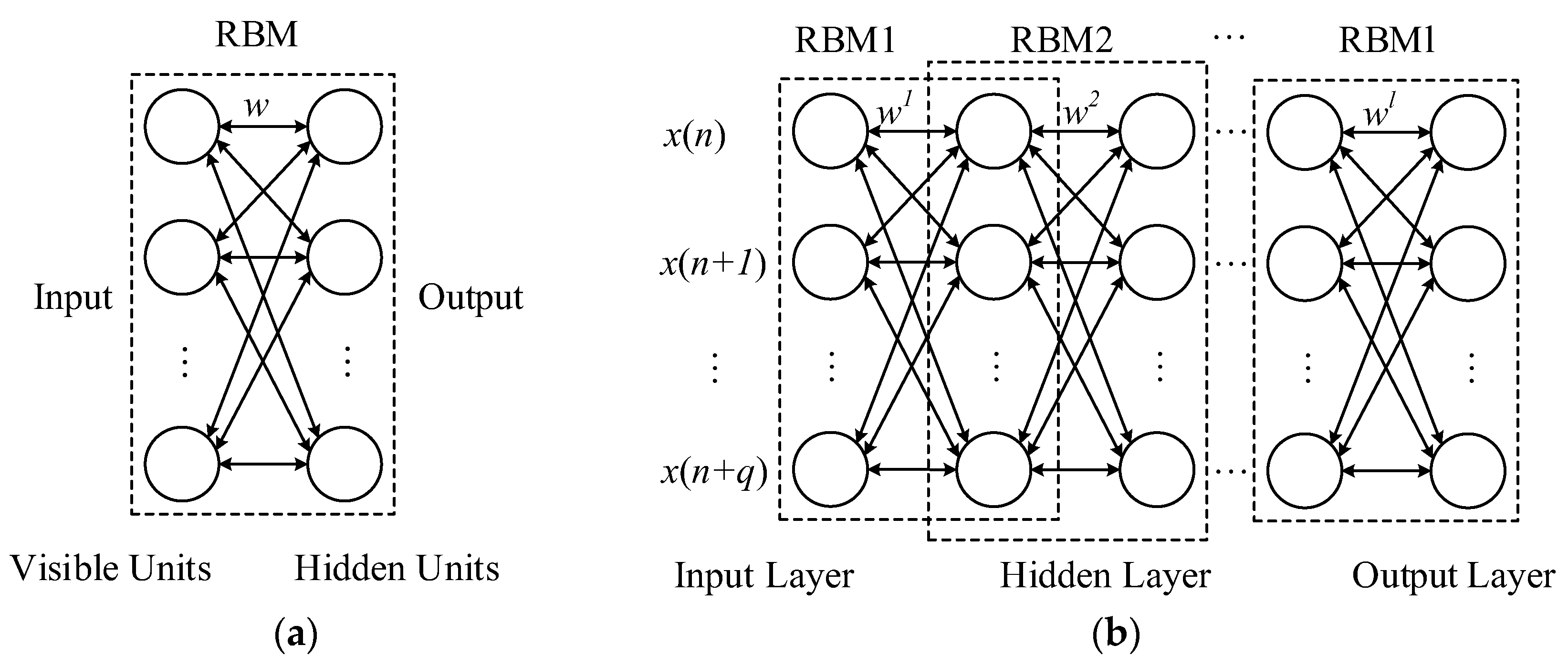
A DBN is stacked by multiple restricted Boltzmann machine (RBM) layers, and their structure are shown in Figure 1. As seen in Figure 1a, a RBM is composed of one visible layer and one hidden layer. Symmetrically weighted connections are present among the units of interlayers, and no connections occur between the neurons in the same layer [34]. As shown in Figure 1b, a DBN is stacked by l RBMs, which presents one input layer, also named visible layer, multiple hidden layers and one output layer. The visible layer of the first RBM acts as the DBN input layer; the hidden layer of the first RBM is the visible layer of the second RBM and is the first hidden layer of the DBN. Then, the hidden layer of the second RBM is the visible layer of the third RBM and the second hidden layer of DBN. This process continues, and layer-by-layer stacking occurs. Thus, a DBN with multiple hidden layers is established.

Hinton et al. [12] proposed a fast, unsupervised and greedy learning method for DBN. This learning process is based on the training one layer at a time. The main concept of this algorithm is that the input samples are randomly selected for training the first RBM, and the hidden units can acquire the unique important features of the input samples. We used the hidden layer as the first hidden layer of DBN, the training feature is used as input samples to train the next RBM. We repeated the process of the learning feature until all layers of DBN have been trained over.

The classic RBM model can only address binary-valued data. A continuous restricted Boltzmann machine (CRBM) was proposed by Chen and Murray [35], and the neurons indicate continuous state values. Therefore, the model can address real-valued data. Given that daily urban water demand data are continuous, we used multiple CRBMs to construct the DBN, which can process real-valued data and can be applied to urban daily water demand forecasting. The model training process is described as follows:

Step 1:

The state of units and the weight matrix are randomly initialized. Let $s_v$ and $s_h$ denote the states of the visible units $v$ and hidden units $h$, and $w_{vh}$ is the interconnected weight.

Step 2:

A set of training sample are randomly selected as input; the states $s_h$ of the first hidden units are updated based on the following formula:

$$s_h={\phi }_h\left[{\displaystyle \sum _v{w}_{vh}{s}_v+\sigma \cdot N_h(0,1)}\right]$$

(8)

with

$${\phi }_h(x_h)={\theta }_{\min }+({\theta }_{\max }-{\theta }_{\min })\cdot \frac{1}{1+e^{-a_h{x}_h}}$$

(9)

where $\sigma$ represents a constant between 0 and 1, $N_h(0,1)$ denotes a Gaussian random unit with a unit variance and zero mean, ${\phi }_h(x)$ is a sigmoid function with asymptotes at ${\theta }_{\min }$ and ${\theta }_{\max }$, and $a_h$ controls the gradient of the sigmoid function and the nature of the unit’s random behavior [36].

Step 3:

$s_h$ is used in computing the states $s_v^{\prime }$ of visible units:

$$s_v^{\prime }={\phi }_v\left[{\displaystyle \sum _h{w}_{vh}{s}_h+\sigma \cdot N_v(0,1)}\right]$$

(10)

Step 4:

$s_v^{\prime }$ is used in computing the states $s_h^{\prime }$ of hidden units:

$$s_h^{\prime }={\phi }_h\left[{\displaystyle \sum _v{w}_{vh}{s}_v^{\prime }+\sigma \cdot N_h(0,1)}\right]$$

(11)

Step 5:

The next set of training sample is randomly selected and Step 2 commences. If all training samples are used, the following formulas are used in updating the weight and noise control parameters:

$$\Delta w_{vh}={\eta }_w\left(<s_v{s}_h>-<s_v^{\prime }{s}_h^{\prime }>\right)$$

(12)

$$\Delta a_h=\frac{{\eta }_a}{a_h^2}\left(<s_h^2>-<s_h^{\prime 2}>\right)$$

(13)

$$w_{vh}(k+1)=w_{vh}(k)+\Delta w_{vh}$$

(14)

$$a_h(k+1)=a_h(k)+\Delta a_h$$

(15)

where ${\eta }_w$ and ${\eta }_a$ are the learning rates; $s_v^{\prime }$ and $s_h^{\prime }$ are the single-step sampled state of unit $v$ and $h$, respectively; and $<\cdot >$ related to the mean over the training samples.

Step 6:

Step 2 is repeated, and the next round of training is conducted until the number of preset training is reached or the weight change matrix is sufficiently small, that is, $|\Delta w(k)|<\epsilon$, and the first CRBM is trained over.

Step 7:

The output of the first CRBM is considered as the input of the second CRBM. Steps 1–6 are repeated for training the second CRBM until all CRBMs of DBN are trained and the training is completed.

2.3. The DSDBN Forecasting Model

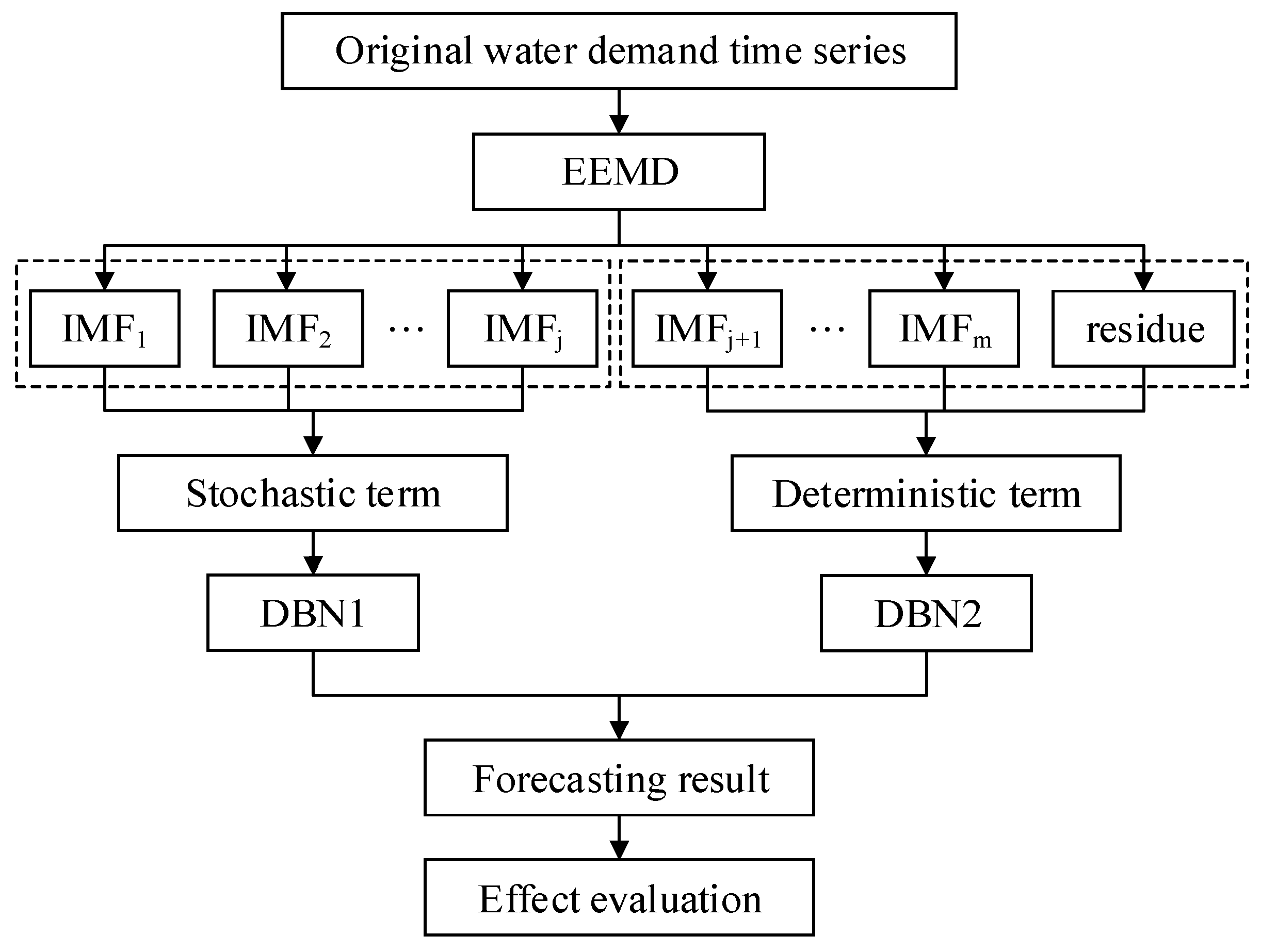
Daily urban water demand time series is a typical nonlinear and non-stationary signal. We used EEMD to extract the IMFs and residue component in the original time series of daily water demand. We reconstructed the stochastic term and deterministic term in accordance with the frequency characteristic, thereby decreasing the non-stationary of the original data. Then, we used DBN to predict the two feature terms. Finally, the prediction results of the two feature term were superimposed. The modeling structure flow chart of the DSDBN prediction model is illustrated in Figure 2.

As seen in Figure 2, the six main steps of the DSDBN forecasting method are listed as follows:

Step 1:

Daily water demand time series is collected, and data outliers are eliminated.

Step 2:

EEMD is utilized to decompose the daily water demand time series into the combination of m IMFs and one residue component.

Step 3:

GFT is performed to analyze the spectral characteristics of each IMF and residue. The stochastic term $x_{\mathrm{sto}}(t)$ and deterministic term $x_{\det }(t)$ are reconstructed in accordance with the frequency characteristic.

Step 4:

The structure of the DBN model is designed to correspondingly predict the stochastic term $x_{\mathrm{sto}}(t)$ and deterministic term $x_{\det }(t)$, including selecting the number of input units, hidden units and layer and setting other parameters.

Step 5:

The prediction results of the stochastic term and the deterministic term are combined. The results can be used as the final prediction result for the original daily water demand time series.

Step 6:

The final result is compared with the peer model, and the performance of the proposed DSDBN model is evaluated.

3. Case Study

3.1. Study Area and Data

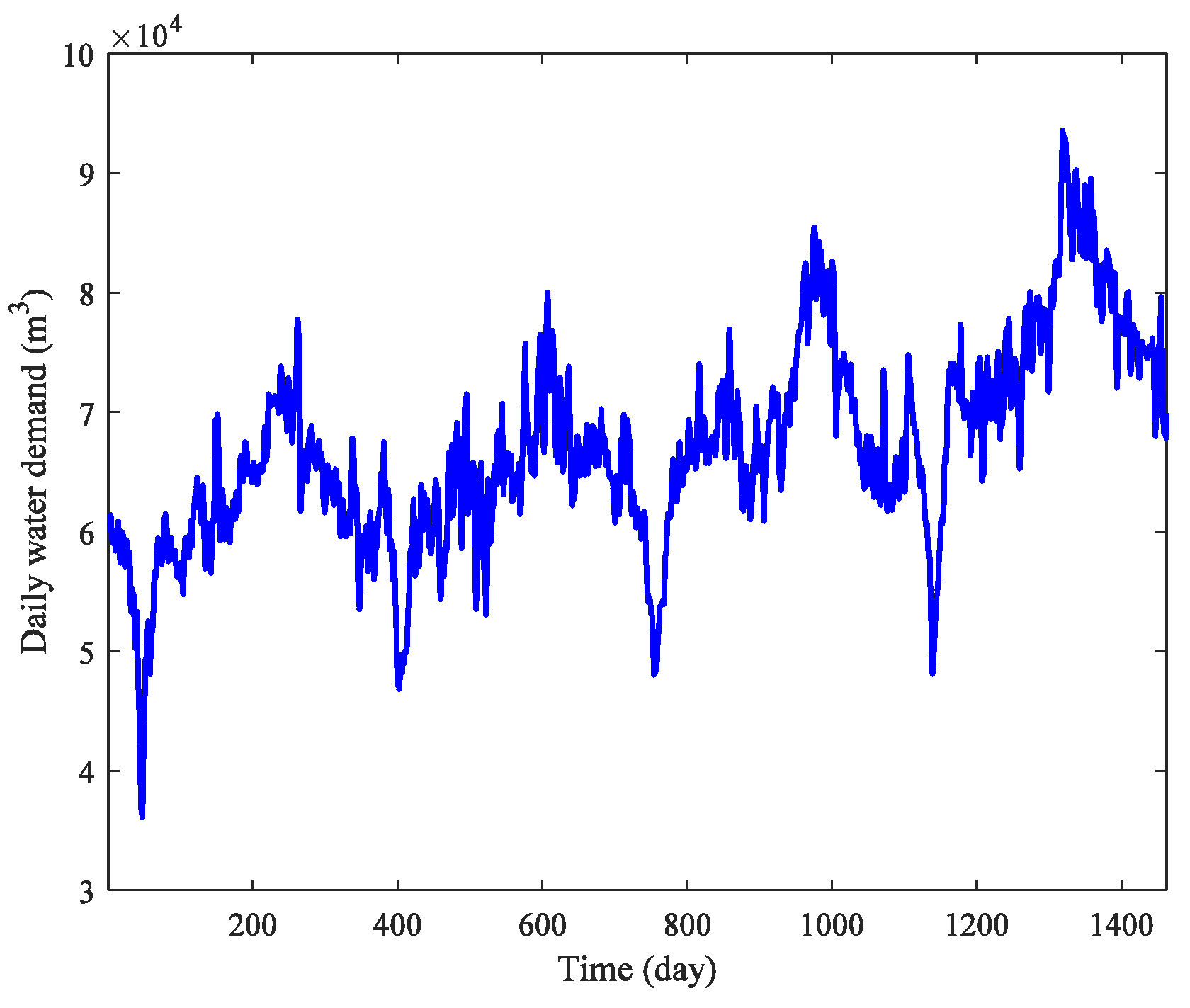
We collected 1462 daily water demand records from 1 January 2012 to 1 January 2016 from an urban waterworks (latitude and longitude north 113.158037, east 27.824564) in Zhuzhou, China. This urban waterworks has a capacity of 100,000 m³ of filter water per day and supplies water for approximately 0.4 million people and enterprises in Lusong District, an area of approximately 200 km². Among 1462 daily records, the first 1224 daily series from 1 January 2012 to 8 May 2015 were used as the training dataset, and the other 238 records were retained for testing. The original daily urban water demand data are plotted in Figure 3.

As shown in Figure 3, the daily water demand time series indicates a certain regularity as time continues. The water demand begins to decrease until the annual minimum in the winter, then increase. The highest value is reached in the summer because most enterprises indicate that their main water consumers are on holiday and decrease their water demand during China’s Spring Festival.

3.2. Performance Evaluation

For validating and evaluating the forecasting performance of the proposed models, we used four widely used criteria in this study.

3.2.1. Mean Absolute Percentage Error (MAPE)

MAPE is an unbiased estimator for evaluating the forecasting capability of a model and it is often applied to practice because of its intuitive explanation in terms of relative error [37]. MAPE is used in evaluating the effect of the model from the perspective of the prediction error.

$$\mathrm{MAPE}=\frac{100}{N}{\displaystyle \sum _{t=1}^N\left|\frac{Y(t)-\widehat{Y}(t)}{Y(t)}\right|}$$

(16)

where $Y(t)$ and $\widehat{Y}(t)$ denote the observed and predicted value at time $t$, respectively, and $N$ is the number of observed value. A low value indicates good prediction effect of the model.

3.2.2. Normalized Root-Mean-Square Error (NRMSE)

NRMSE represents the total accuracy of the prediction [11].

$$\mathrm{NRMSE}=\frac{\sqrt{\frac{1}{N}{\displaystyle \sum _{t=1}^N{\left[Y(t)-\widehat{Y}(t)\right]}^2}}}{\frac{1}{N}{\displaystyle \sum _{t=1}^{N}Y(t)}}$$

(17)

A lower value indicates less residual variance and stronger agreement between the observed and predicted values.

3.2.3. Correlation Coefficient (CC)

CC shows the linear between the observed and predicted value [38].

$$\mathrm{CC}=\frac{{\displaystyle \sum _{t=1}^N\left[Y(t)-\overline{Y}(t)\right]\left[\widehat{Y}(t)-\overline{\widehat{Y}}(t)\right]}}{\sqrt{{\displaystyle \sum _{t=1}^N{\left[Y(t)-\overline{Y}(t)\right]}^2}}\sqrt{{\displaystyle \sum _{t=1}^N{\left[\widehat{Y}(t)-\overline{\widehat{Y}}(t)\right]}^2}}}$$

(18)

where $\overline{Y}(t)$ and $\overline{\widehat{Y}}(t)$ are the means of the observed and the predicted value, respectively.

A CC value approaching 1 indicates a good fit between the observed and predicted value and superior predictive capability of the model.

3.2.4. Determination Coefficient (DC)

DC shows the unconformity between the observed and predicted values and the number of points close to the bisector in the scatter plot of two variables [39].

$$\mathrm{DC}=1-\frac{{\displaystyle \sum _{t=1}^N{\left[Y(t)-\widehat{Y}(t)\right]}^2}}{{\displaystyle \sum _{t=1}^N{\left[Y(t)-\overline{Y}(t)\right]}^2}}$$

(19)

According to Equation (19), ${\displaystyle \sum _{t=1}^N{\left[Y(t)-\widehat{Y}(t)\right]}^2}=0$ and DC = 1 indicate ideal performance of the model.

4. Results and Discussion

4.1. Decomposing and Reconstructing Water Demand Time Series

Using EEMD to decompose the original water demand time series, two key parameters need to be set, namely, the numbers of the ensemble $M$ and the amplitude of white noise $e$. As presented in Equation (5), Wu and Huang [29] set the amplitude of added white noise signal to 0.2 times the standard deviation and experimented with empirical methods for numerous times. The group encountered difficulty in eliminating the mode mixing phenomenon at extremely small values of $e$, whereas, at an excessively large $e$, they observed that several extra IMF components are produced, leading to misjudgment of the results. The EEMD parameter settings for different application areas [40,41,42] refer to the method proposed by Wu and Huang [29]. In this study, the ensemble member $M$ and the standard deviation of added white noise signal $e^{\prime }$ of the EEMD were set to 100 and 0.2, respectively.

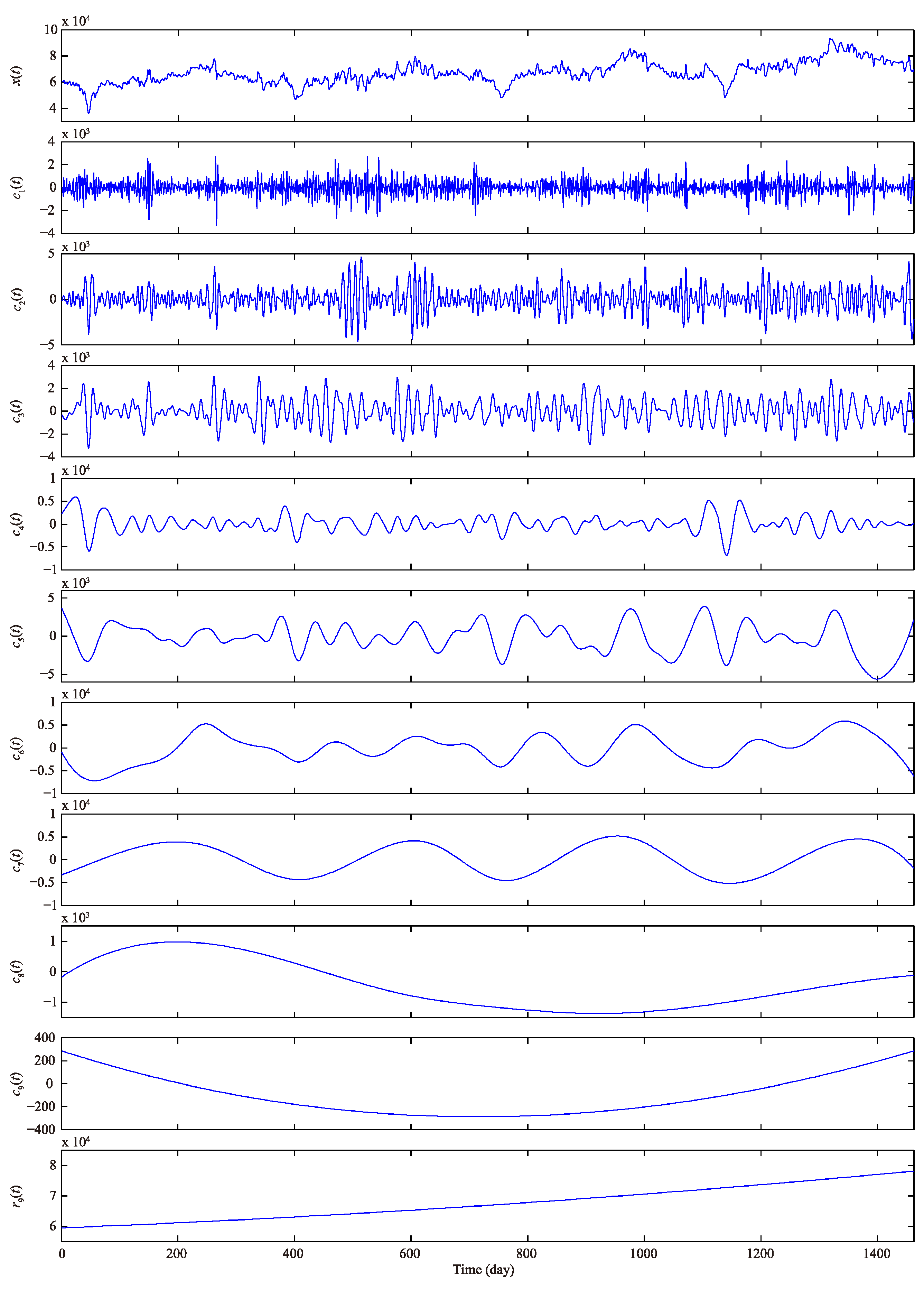
As described above, the original daily urban water demand time series is decomposed into nine independent IMF $c_1\left(t\right)$–$c_9\left(t\right)$ and one residue $r_9\left(t\right)$ by using the EEMD method, the decomposition results are shown in Figure 4, where the components $c_1\left(t\right)$–$c_9\left(t\right)$ and $r_9\left(t\right)$ are in accordance with the order from high to low frequency, and $r_9\left(t\right)$ reflects the overall trend of the original daily water demand time series. The EEMD decomposition presents significant physical meaning, transforms nonlinear and non-stationary series into stationary series and facilitates improved forecasting performance.

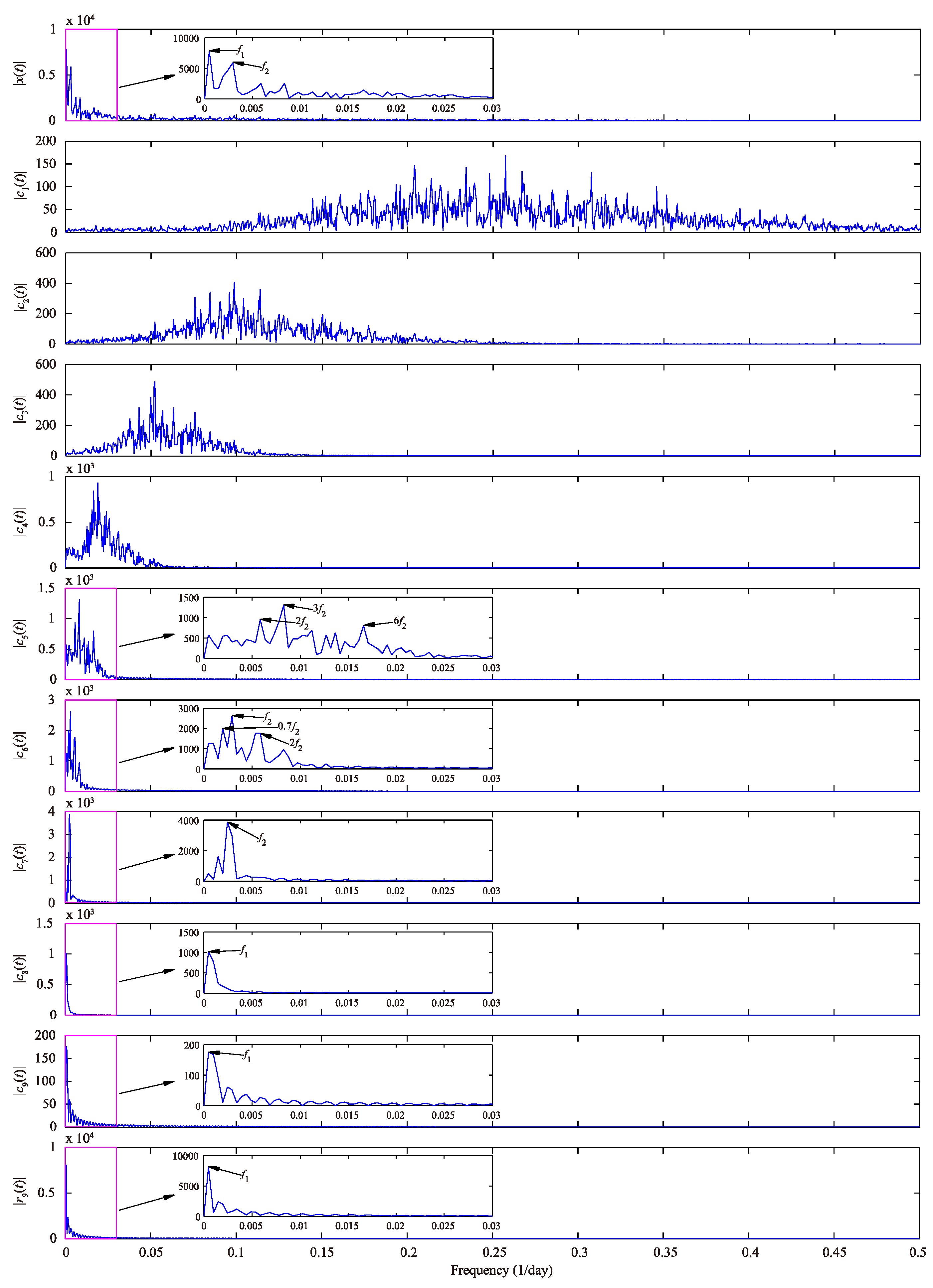
The frequency spectrum of each IMF and residue component using GFT are shown in Figure 5, wherein two main frequency components, namely, $f_1=0.000488$ (1/day) and $f_2=0.002930$ (1/day), are in the original daily water demand time series; different frequency components are present in $c_1\left(t\right)$–$c_4\left(t\right)$; similar frequency components $f_2$ in $c_5\left(t\right)$–$c_7\left(t\right)$ ($2f_2$, $3f_2$ and $6f_2$ in $c_5\left(t\right)$; $0.7f_2$, $f_2$ and $2f_2$ in $c_6\left(t\right)$; and $f_2$ in $c_7\left(t\right)$); and same frequency components $f_1$ in $c_8\left(t\right)$, $c_9\left(t\right)$ and $r_9\left(t\right)$. According to EEMD and GFT analysis results, the nine IMFs and one residue component can be reconstructed into three categories, namely, ${\displaystyle \sum _{i=1}^4{c}_i\left(t\right)}$, ${\displaystyle \sum _{i=5}^7{c}_i\left(t\right)}$ and $c_8\left(t\right)+c_9\left(t\right)+r_9\left(t\right)$. The first category can be regarded as the stochastic term, whereas the latter two categories are treated as deterministic terms, that is, stochastic term $x_{\mathrm{sto}}(t)={\displaystyle \sum _{i=1}^4{c}_i\left(t\right)}$ and deterministic term $x_{\det }(t)={\displaystyle \sum _{i=5}^9{c}_i\left(t\right)}+r_9(t)$.

4.2. Modeling Method of DBN

The number of input nodes, hidden layers and nodes is the key issue in the design of DBN structure. The number of input nodes that corresponds to the number of previous observed values is correlated with future values and determines the autocorrelation structure of the daily water demand time series. The hidden layers and nodes expose nonlinear patterns and complex intrinsic relationship in the daily water demand time series. At present, no mature theory can solve these problems. In this study, the number of input nodes, hidden layers and nodes of DBN was determined by the experiment.

Assuming that the training dataset is $x(n)$, we used one-step-ahead forecasting and set the DBN with $q$ input nodes and an output node, with the number of $q$ ranging from 1 to 10. The training sample involves $X(n)=\left[x(n),x(n+1),\dots ,x(n+q)\right]$ as the inputs and $Y(n)=x(n+q+1)$ as the output. The hidden layers were set from 1 to 3, and the number of the hidden nodes were set to 4, 8, 12, 16 and 20. We used the four evaluation criteria described in Section 3.2 to evaluate the learning capability of DBN with different parameters and select the number of hidden layers and nodes with optimal learning performance. Researchers found that the forecasting performance of multiple hidden layers are superior to that with only one layer [43], and that the forecasting performance of the neural network exerts a significant effect as the number of hidden nodes changes [44].

Other parameters need to be set during the DBN training process. First, we set the initial values and update the method of $w_{vh}$ in Equation (8); then, we used a group of random initial values in the first CRBM and constantly adjusted the weight matrix until stability was achieved. Then, the weight matrix of the next CRBM was initialized using the weight matrix of the previous CRBM, and layer-by-layer training was conducted until the CRBM trainings were finished. The parameters ${\theta }_{\max }$ and ${\theta }_{\min }$ in Equation (9) were set to be the maximum and minimum values of the entire training samples, respectively. The parameters $\sigma$ in Equations (10) and (11), ${\eta }_w$ in Equation (12), and ${\eta }_a$ and $a_h$ in Equation (13) were determined by 5-fold cross-validation method. To obtain the global optimal solution, we trained every DBN 20 times using 20 groups of random initial values, and the mean values of those 20 times were used as the training result of a DBN.

The stochastic term $x_{\mathrm{sto}}(t)$ and deterministic term $x_{\det }(t)$ were modeled using the method described above. According to the four performance evaluation criteria, namely, MAPE, NRMSE, CC and DC, the best structure of DBN with the best learning performance was selected. The structure of DBN and the forecasting performance of training dataset are listed in

Table 1. DBN structure and the forecasting result of training dataset.

Feature Term	DBN Structure	MAPE	NRMSE	CC	DC
$x_{\mathrm{sto}}(t)$	10-8-12-1	7.591709	0.089303	0.904627	0.818234
$x_{\det }(t)$	4-16-1	0.387461	0.003663	0.999941	0.999882

, where the optimal architecture of DBN for the stochastic term $x_{\mathrm{sto}}(t)$ is 10-8-12-1, that is, DBN with 2 hidden layers, 10 input nodes, 8 and 12 nodes in the first hidden layer and second hidden layer, respectively, and 1 output node. For the deterministic term $x_{\det }(t)$, the optimal structure of DBN is 4-16-1 (input layer: 4 nodes, hidden layer: 16 nodes and output: 1 node).

4.3. Forecasting Result

The forecasting result of the stochastic term $x_{\mathrm{sto}}(t)$ and deterministic term $x_{\det }(t)$ is plotted in Figure 6. Figure 6a shows the forecasting result of the stochastic term $x_{\mathrm{sto}}(t)$ using DBN with 10-8-12-1, and Figure 6b plots the forecasting results of the deterministic term $x_{\det }(t)$ using DBN with 4-16-1. The final forecasting results of the original daily water demand can be obtained by superimposing the forecasting results of stochastic term $x_{\mathrm{sto}}(t)$ and deterministic term $x_{\det }(t)$. Figure 7 displays the final forecasting results. Figure 7a shows the comparison between the predicted and observed value, and Figure 7b exhibits the scatter of predicted and observed values. In Figure 7a, the forecasting values can follow the changes of the observed daily water demand. The correlation between the predicted and the observed values in Figure 7b indicates that both values are highly consistent. The results of four performance evaluation criteria are MAPE = 1.291099, NRMSE = 0.016625, CC = 0.976528 and DC = 0.953512, which indicate that the proposed approach exhibits good learning performance and forecasting capability.

4.4. Comparison Experiment

To assess the performance of the proposed DSDBN model, ARIMA model, feed forward neural network (FFNN) model, and SVR model were employed for comparison using the same training and testing samples. The three comparison models also use EEMD method to decompose the daily water demand time series, and the stochastic and deterministic terms are reconstructed using the same method as described in Section 4.1. In addition, for assessing the effect of EEMD on predictive performance, a single DBN model was developed to use the original daily water demand time series. In ARIMA modeling, KPSS is used to test the stability of the two feature terms and Akaike information criterion [45] is employed to identify the best fitted model. FFNN modeling uses the same nodes and layers with the DSDBN model, the sigmoid and linear activation functions in the hidden and output layer, respectively, and the back propagation algorithm to train the model. In SVR modeling, the kernel function selects the linear kernel and uses the grid search method to determine values of optimal parameters $C$ and ${\gamma }^2$, and the value of insensitive loss function ${\epsilon }^{\prime }$ is set to 0.1. The single DBN modeling uses the same method as DSDBN modeling to select the number of nodes and hidden layers, and the structure of single DBN is finally set to 6-4-12-1.

The prediction results of the four different comparison models are shown in

Table 2. Comparison of the predictive performances by using different forecasting models.

Model	MAPE	NRMSE	CC	DC
DSDBN	1.291099	0.016625	0.976528	0.953512
EEMD-ARIMA	5.489027	0.058402	0.964553	0.426299
EEMD-FFNN	1.972864	0.027913	0.954584	0.868948
EEMD-SVR	4.274470	0.049398	0.965657	0.589553
DBN	1.621183	0.020369	0.968261	0.930088

. In Table 2, the DSDBN model presents smallest MAPE and NRMSE values, and the largest CC and DC values among the models and improved the EEMD-ARIMA, EEMD-FFNN, EEMD-SVR and DBN models, with reduction of MAPE of approximately 76.48%, 34.56%, 69.8% and 20.36%, respectively; reduction of NRMSE of 71.53%, 40.44%, 66.34% and 18.38%, respectively; increase in CC of 1.24%, 2.3%, 1.13% and 0.85%, respectively; and increase in DC of 123.67%, 9.73%, 61.73% and 2.52%, respectively. The results of this analysis illustrate that the proposed DSDBN model is superior to the other four models in forecasting daily urban water demand. Moreover, the findings indicate that the DSDBN model, which is based on the method of “decomposing and reconstructing”, improves the prediction accuracy compared with the single DBN model; thus, the model is superior to ARIMA, FFNN and SVR models in predicting nonlinear and non-stationary daily urban water demand.

5. Conclusions

In this paper, a novel dual-scale deep belief network method is proposed to predict the daily urban water demand. The proposed approach is exploited using the historical daily water demand datasets from an urban waterworks in Zhuzhou, China. By using EEMD method, the original daily urban water demand data are decomposed into nine IMFs and one residue component, and reconstructed into stochastic and deterministic terms according to the frequency characteristics of each component by GFT analysis. DBN models are used to forecast these two feature terms. Then, the two sub-results are superposed to produce the final forecasting results. To validate and assess the forecasting performance of the proposed model, EEMD-ARIMA, EEMD-FFNN, EEMD-SVR and single DBN models were employed as benchmark comparisons. Four standard performance evaluation criteria (MAPE, NRMSE, CC and DC) were utilized to evaluate the forecasting capacity of all the selected models. Results of the empirical study show that the DSDBN approach exhibits the highest prediction accuracy among all comparison models on daily water demand forecasting of the urban waterworks in Zhuzhou, China.

References

- House-Peters, L.A.; Chang, H. Urban water demand modeling: Review of concepts, methods, and organizing principles. Water Resour. Res. 2011, 47, W05401. [Google Scholar] [CrossRef]
- Donkor, E.A.; Mazzuchi, T.A.; Soyer, R.; Roberson, J.A. Urban water demand forecasting: Review of methods and models. J. Water Resour. Plan. Manag. 2014, 140, 146–159. [Google Scholar] [CrossRef]
- Jain, A.; Ormsbee, L.E. Short-term water demand forecast modeling techniques-conventional methods versus ai. J. AWWA 2002, 94, 64–72. [Google Scholar] [CrossRef]
- Gato, S.; Jayasuriya, N.; Roberts, P. Temperature and rainfall thresholds for base use urban water demand modelling. J. Hydrol. 2007, 337, 364–376. [Google Scholar] [CrossRef]
- Di, T.; Martinez, C.J.; Asefa, T. Improving short-term urban water demand forecasts with reforecast analog ensembles. J. Water Resour. Plan. Manag. 2016, 142, 1–11. [Google Scholar]
- Msiza, I.S.; Nelwamondo, F.V.; Marwala, T. Artificial neural networks and support vector machines for water demand time series forecasting. In Proceedings of the IEEE International Conference on Systems, Man and Cybernetics, Montreal, QC, Canada, 7–10 October 2007; pp. 638–643. [Google Scholar]
- Herrera, M.; Torgo, L.; Izquierdo, J.; Pérez-García, R. Predictive models for forecasting hourly urban water demand. J. Hydrol. 2010, 387, 141–150. [Google Scholar] [CrossRef]
- Adamowski, J.; Fung Chan, H.; Prasher, S.O.; Ozga-Zielinski, B.; Sliusarieva, A. Comparison of multiple linear and nonlinear regression, autoregressive integrated moving average, artificial neural network, and wavelet artificial neural network methods for urban water demand forecasting in montreal, canada. Water Resour. Res. 2012, 48, W01528. [Google Scholar] [CrossRef]
- Chen, G.; Long, T.; Xiong, J.; Bai, Y. Multiple random forests modelling for urban water consumption forecasting. Water Resour. Manag. 2017, 31, 4715–4729. [Google Scholar] [CrossRef]
- Tiwari, M.K.; Adamowski, J. Urban water demand forecasting and uncertainty assessment using ensemble wavelet-bootstrap-neural network models. Water Resour. Res. 2013, 49, 6486–6507. [Google Scholar] [CrossRef]
- Bai, Y.; Wang, P.; Li, C.; Xie, J.; Wang, Y. A multi-scale relevance vector regression approach for daily urban water demand forecasting. J. Hydrol. 2014, 517, 236–245. [Google Scholar] [CrossRef]
- Hinton, G.E.; Osindero, S.; Teh, Y.W. A fast learning algorithm for deep belief nets. Neural Comput. 2006, 18, 1527–1554. [Google Scholar] [CrossRef] [PubMed]
- Kuremoto, T.; Kimura, S.; Kobayashi, K.; Obayashi, M. Time series forecasting using a deep belief network with restricted boltzmann machines. Neurocomputing 2014, 137, 47–56. [Google Scholar] [CrossRef]
- Mohamed, A.R.; Dahl, G.E.; Hinton, G. Acoustic modeling using deep belief networks. IEEE Trans. Audio Speech Lang. Proc. 2012, 20, 14–22. [Google Scholar] [CrossRef]
- Sarikaya, R.; Hinton, G.E.; Deoras, A. Application of deep belief networks for natural language understanding. IEEE/ACM Trans. Audio Speech Lang. Proc. 2014, 22, 778–784. [Google Scholar] [CrossRef]
- Chen, Y.; Zhao, X.; Jia, X. Spectral–spatial classification of hyperspectral data based on deep belief network. IEEE J. Sel. Top. Appl. Earth Obs. Remote Sens. 2015, 8, 2381–2392. [Google Scholar] [CrossRef]
- Tang, B.; Liu, X.; Lei, J.; Song, M.; Tao, D.; Sun, S.; Dong, F. Deepchart: Combining deep convolutional networks and deep belief networks in chart classification. Signal Proc. 2016, 124, 156–161. [Google Scholar] [CrossRef]
- Shao, H.; Jiang, H.; Zhang, H.; Liang, T. Electric locomotive bearing fault diagnosis using novel convolutional deep belief network. IEEE Trans. Ind. Electron. 2017, 65, 2727–2736. [Google Scholar] [CrossRef]
- Zhang, Z.; Zhao, J. A deep belief network based fault diagnosis model for complex chemical processes. Comput. Chem. Eng. 2017, 107, 395–407. [Google Scholar] [CrossRef]
- Shen, F.; Chao, J.; Zhao, J. Forecasting exchange rate using deep belief networks and conjugate gradient method. Neurocomputing 2015, 167, 243–253. [Google Scholar] [CrossRef]
- Zheng, J.; Fu, X.; Zhang, G. Research on exchange rate forecasting based on deep belief network. Neural Comput. Appl. 2017. [Google Scholar] [CrossRef]
- Bai, Y.; Chen, Z.; Xie, J.; Li, C. Daily reservoir inflow forecasting using multiscale deep feature learning with hybrid models. J. Hydrol. 2016, 532, 193–206. [Google Scholar] [CrossRef]
- Dedinec, A.; Filiposka, S.; Dedinec, A.; Kocarev, L. Deep belief network based electricity load forecasting: An analysis of macedonian case. Energy 2016, 115, 1688–1700. [Google Scholar] [CrossRef]
- Li, C.; Ding, Z.; Yi, J.; Lv, Y.; Zhang, G. Deep belief network based hybrid model for building energy consumption prediction. Energies 2018, 11, 242. [Google Scholar] [CrossRef]
- Wang, H.Z.; Wang, G.B.; Li, G.Q.; Peng, J.C.; Liu, Y.T. Deep belief network based deterministic and probabilistic wind speed forecasting approach. Appl. Energy 2016, 182, 80–93. [Google Scholar] [CrossRef]
- Huang, N.E.; Shen, Z.; Long, S.R.; Wu, M.C.; Shih, H.H.; Zheng, Q.; Yen, N.-C.; Tung, C.C.; Liu, H.H. The empirical mode decomposition and the hilbert spectrum for nonlinear and non-stationary time series analysis. Proc. Math. Phys. Eng. Sci. 1998, 454, 903–995. [Google Scholar] [CrossRef]
- Huang, N.E.; Shen, Z.; Long, S.R. A new view of nonlinear water waves: The hilbert spectrum. Ann. Rev. Fluid Mech. 1999, 31, 417–457. [Google Scholar] [CrossRef]
- Liu, Z.; Sun, W.; Zeng, J. A new short-term load forecasting method of power system based on eemd and ss-pso. Neural Comput. Appl. 2014, 24, 973–983. [Google Scholar] [CrossRef]
- Wu, Z.; Huang, N.E. Ensemble empirical mode decomposition: A noise-assisted data analysis method. Adv. Adapt. Data Anal. 2009, 1, 1–41. [Google Scholar] [CrossRef]
- Wang, W.C.; Chau, K.W.; Qiu, L.; Chen, Y.B. Improving forecasting accuracy of medium and long-term runoff using artificial neural network based on eemd decomposition. Environ. Res. 2015, 139, 46–54. [Google Scholar] [CrossRef] [PubMed]
- Wang, S.; Zhang, N.; Wu, L.; Wang, Y. Wind speed forecasting based on the hybrid ensemble empirical mode decomposition and ga-bp neural network method. Renew. Energy Int. J. 2016, 94, 629–636. [Google Scholar] [CrossRef]
- Box, G.E.P.; Jenkins, G.M.; Reinsel, G.C.; Ljung, G.M. Time Series Analysis: Forecasting and Control, 5th ed.; Wiley: Hoboken, NJ, USA, 2015. [Google Scholar]
- Cheng, J.; Yang, Y.; Yu, D. The envelope order spectrum based on generalized demodulation time–frequency analysis and its application to gear fault diagnosis. Mech. Syst. Signal Process. 2010, 24, 508–521. [Google Scholar] [CrossRef]
- Teh, Y.W.; Hinton, G.E. Rate-coded restricted boltzmann machines for face recognition. In Proceedings of the 13th International Conference on Neural Information Processing Systems; MIT Press: Denver, CO, USA, 2000; pp. 872–878. [Google Scholar]
- Chen, H.; Murray, A.F. Continuous restricted boltzmann machine with an implementable training algorithm. IEE Proc. Vis. Image Signal Process. 2003, 150, 153–158. [Google Scholar] [CrossRef]
- Chen, H.; Murray, A. A continuous restricted boltzmann machine with a hardware- amenable learning algorithm. In Proceedings of 12th International Conference on Artificial Neural Networks; Springer: Madrid, Spain, 2002; pp. 358–363. [Google Scholar]
- De Myttenaere, A.; Golden, B.; Le Grand, B.; Rossi, F. Mean absolute percentage error for regression models. Neurocomputing 2016, 192, 38–48. [Google Scholar] [CrossRef]
- Rathinasamy, M.; Khosa, R. Multiscale nonlinear model for monthly streamflow forecasting: A wavelet-based approach. J. Hydroinform. 2012, 14, 424–442. [Google Scholar] [CrossRef]
- Nash, J.E.; Sutcliffe, J.V. River flow forecasting through conceptual models part i—A discussion of principles. J. Hydrol. 1970, 10, 282–290. [Google Scholar] [CrossRef]
- Lei, Y.; He, Z.; Zi, Y. Eemd method and wnn for fault diagnosis of locomotive roller bearings. Expert Syst. Appl. 2011, 38, 7334–7341. [Google Scholar] [CrossRef]
- Tang, L.; Yu, L.; Wang, S.; Li, J.; Wang, S. A novel hybrid ensemble learning paradigm for nuclear energy consumption forecasting. Appl. Energy 2012, 93, 432–443. [Google Scholar] [CrossRef]
- Xu, X.; Niu, D.; Zhang, L.; Wang, Y.; Wang, K. Ice cover prediction of a power grid transmission line based on two-stage data processing and adaptive support vector machine optimized by genetic tabu search. Energies 2017, 10, 1862. [Google Scholar] [CrossRef]
- Le Roux, N.; Bengio, Y. Representational power of restricted boltzmann machines and deep belief networks. Neural Comput. 2008, 20, 1631–1649. [Google Scholar] [CrossRef] [PubMed]
- Zhang, G.; Hu, M.Y. Neural network forecasting of the british pound/us dollar exchange rate. Omega 1998, 26, 495–506. [Google Scholar] [CrossRef]
- Akaike, H. A new look at the statistical model identification. IEEE Trans. Autom. Control 1974, 19, 716–723. [Google Scholar] [CrossRef]
Figure 1.
Structural illustration: (a) RBM structure; and (b) DBN structure.
Figure 2.
Modeling structure flow chart of the DSDBN model.
Figure 3.
Original daily urban water demand time series for 1 January 2012–1 January 2016.
Figure 4.
Decomposition results using EEMD method.
Figure 5.
Frequency spectrum of each IMF and residue component using GFT.
Figure 6.
Forecasting results of the two feature terms: (a) stochastic term ; and (b) deterministic term .
Figure 7.
Final forecasting results of the daily water demand: (a) comparison between the predicted value and the observed value; and (b) the scatter of the predicted value and the observed value.