Electricity Purchase Optimization Decision Based on Data Mining and Bayesian Game

1
State Key Laboratory of Alternate Electrical Power System with Renewable Energy Sources, North China Electric Power University, Baoding 071003, China
2
Department of automation, North China Electric Power University, Baoding 071003, China
3
State Grid Jiangsu Electric Power Co., Ltd., Suzhou Power Supply Branch, Suzhou 215004, China
*
Authors to whom correspondence should be addressed.
Energies 2018, 11(5), 1063; https://doi.org/10.3390/en11051063
Submission received: 29 March 2018
/
Revised: 16 April 2018
/
Accepted: 20 April 2018
/
Published: 26 April 2018
Abstract
:The openness of the electricity retail market results in the power retailers facing fierce competition in the market. This article aims to analyze the electricity purchase optimization decision-making of each power retailer with the background of the big data era. First, in order to guide the power retailer to make a purchase of electricity, this paper considers the users’ historical electricity consumption data and a comprehensive consideration of multiple factors, then uses the wavelet neural network (WNN) model based on “meteorological similarity day (MSD)” to forecast the user load demand. Second, in order to guide the quotation of the power retailer, this paper considers the multiple factors affecting the electricity price to cluster the sample set, and establishes a Genetic algorithm- back propagation (GA-BP) neural network model based on fuzzy clustering (FC) to predict the short-term market clearing price (MCP). Thirdly, based on Sealed-bid Auction (SA) in game theory, a Bayesian Game Model (BGM) of the power retailer’s bidding strategy is constructed, and the optimal bidding strategy is obtained by obtaining the Bayesian Nash Equilibrium (BNE) under different probability distributions. Finally, a practical example is proposed to prove that the model and method can provide an effective reference for the decision-making optimization of the sales company.
1. Introduction
Making a comprehensive survey of the market-oriented electricity reforms of various countries—although the national conditions and the paths of reform are all different—opening up the electricity-side market, and giving users the right of free choice have always been core factors in electricity market reform. The gradual opening up of the retail-side market is mainly by introducing the competition through releasing users’ options, allowing users to freely choose to trade with power-retailing or power-generating enterprises, or participating in the wholesale market directly [1,2]. EU countries in 2007 completed the reform of the full liberalization of user options. The USA has achieved retail competition in some states, including its residents. Japan has postponed the retail competition reform that allowing residents to choose their own options. After the earthquake, they formulated a plan for a new power reform and implemented a full-scale retail competition after 2016. Viewing the process of power-retailed side releasing, most countries are in accordance with the voltage level and capacity, phased from large users to gradually release the user option [3].
There are seven major power exchanges in the world currently, of which the European Energy Exchange (EEX) is the largest power exchange with an average daily transaction volume of 170,000 MW. In 2014 alone, the power trade with EEX reached an astonishing 1952 tWh. The Pennsylvania New Jersey Maryland (PJM) exchange in the USA is currently responsible for the operation and management of power systems in 13 U.S. states and the District of Columbia. As a regional Independent system operation (ISO), PJM is responsible for centrally dispatching the largest and most complex power control area in the USA and ranks third in the world in scale. The PJM controlled area accounts for 8.7% of the total population (about 23 million), load 7.5%, installed capacity of 8% (about 58,698 MW), and transmission lines up to more than 12,800 kilometers [4]. The effective application of power big data for the profitability and control of power companies has a high value. Some experts have said that whenever the data utilization increases by 10%, it can cause the power grid to increase profits by 20% to 49%. In the face of a huge power system, data needs to be processed quickly, hence data mining technology came into being, and will play a key role in supporting the sales company to participate in market competition.
Power-selling is the pillar business of the retailer. As an intermediate link between production and use, the power retailer needs to analyze the users’ needs and predict the user’s load demand based on the users’ historical electricity consumption data, considering industry, meteorology, regional economy, related industries, and other factors, so that this can guide the retailer to develop electricity purchase. In recent years, numerous scholars have put forward many effective load forecasting methods. Vilar, J. et al. provided two procedures to obtain prediction intervals for electricity demand and price based on functional data. The first method used a nonparametric autoregressive model and the second one used a partial linear semi-parametric model, in which exogenous scalar covariates are incorporated in a linear way. Also, the residual-based bootstrap algorithms were used in both cases [5]. Zhang, P. et al. combined the gray model and the neural network, chose the gray model according to the historical data, and used the neural network to fit the different model combinations. The combination algorithm improved the prediction accuracy [6]. Ak, R. et al. considered the uncertainty of wind power output and established a model for evaluating the adequacy assessment of the wind integrated system [7]. Based on the massive data of the Intelligent Industrial Park, Wang, B.Y. et al. combined the local weighted linear regression prediction algorithm and the cloud computing Map Reduce model to study the short-term power load forecasting and improve the accuracy of prediction [8]. Bessec, M. et al. analyzed the advantages of wavelet transform methods and studied the benefits of combining predictions with a single model. Each sub-module was then individually predicted and summarized to get the final result [9]. At present, the application of prediction software in the USA is very wide. PJM has a set of independent power market management and operation systems. People in the PJM control center by inputting various factors that affect load, using specialized prediction algorithms and supporting subsystems can accurately predict the power load.
Short-term forecasting of electricity price plays a central role in the electricity market. If market participants can predict electricity prices accurately in advance, they will be in a good position in market competition. For the power retailers, they can use the predicted price to make bidding strategies and optimize quotations, with a view to obtaining greater profits. At present, the research on short-term electricity price is very productive. On the electricity price forecasting (EPF) method, Rafał Weron analyzed the advantages and disadvantages of the previous methods of EPF, and proposed improved suggestions for the shortages. Then he further predicted the development direction of EPF over the next ten years [10]. Silvano Cincotti, et al. analyzed the price of Italian Power Exchange and adopted a discrete-time univariate econometric model, ARMA-GARCH neural network and support vector machine to simulate price time series respectively. By comparing the three methods, they found that the prediction accuracy of the support vector machine method is the highest [11]. Nima Amjady and Farshid Keynia combined wavelet transform and hybrid forecasting to predict the electricity price. They used PJM power market data to compare and verify other EPF methods [12]. Deng, J.J. et al. used ARMA to predict the electricity price. Since the electricity price has heteroscedasticity, the electricity price forecasting model based on ARMA-GARCH was proposed and the accuracy improved [13]. Bento, P.M.R. et al. presented a hybrid method that combines similar and recent day-based selection, correlation, and wavelet analysis in a pre-processing stage. Afterwards a feedforward neural network was used alongside Bat and Scaled Conjugate Gradient Algorithms to improve the traditional neural network learning capability [14]. Neural network is the most used method for short-term EPF. When dealing with EPF, Shi B. et al. and Xing Y. et al. all used cascade neural network (CNN) [15,16]. Wang, D. et al. proposed a hybrid BP model based on fast ensemble empirical mode decomposition (FEEMD), variation mode decomposition (VMD), and firefly algorithm optimization, and used a two-layer decomposition technique to decompose the intrinsic function model into multiple modes to improve prediction accuracy [17]. Hong, Y.Y. et al. proposed a new EPF method that uses empirical model decomposition including correlation coefficients and combines the BP neural network algorithm for short-term EPF [18].
With the increasingly fierce market competition on the power-retail side, sound and optimized power purchase decisions can help retailers win the upper hand and gain higher profits. Gabriel S.A.S. et al. studied the accurate determination of load forecasting, and analyzed the influence of both in connection with the situation of the sales company. Finally, a variety of scenarios under different load predictions were fitted and simulated to obtain different benefits under different scenarios [19]. Bartelj, L.A. et al. and Anderson, E.J.A.B. et al. took into account the influence of factors such as market price and power load when formulating bidding strategies, and designed various scenarios to simulate retailers’ possible revenue and risk in the electricity market transactions [20,21]. Fleten S.E.E. et al. described the different bidding behaviors in the electricity market and analyzed different bidding strategies in the electricity market [22]. Nassiri-Mofakham, F. et al. proposed a new bidding method called multi-attribute portfolio bidding strategy. The model took into account the various factors and market influences of the competing players. This method used the form of an agent to obtain a combination of strategies and quotes that meet the needs of bidders [23]. Hematabadi, A.A. et al. presented a new analytical solution method for Supply Function Equilibrium-based (SFE) bidding strategy in electricity markets. In the inner level, ISO cleared the market to maximize social welfare. In the outer level, each generation company tried to maximize its individual welfare [24]. Dai, Y.M. et al. studied the retailer’s electricity price decision-making problem in power purchase, but did not consider the competition in the retail market environment [25].
With the rapid accumulation of related data, the establishment of a complete power retailer bidding strategy based on data mining technology has become an urgent issue. This paper begins by analyzing the impact of consumer behavior characteristics and preferences on the retailer’s power purchase strategy. First, it uses the WNN method which is based on MSD to predict the user load to develop electricity purchase. Second, it clusters the massive power market data, and establishes a GA-BP neural network prediction model which is based on FC to predict the short-term MCP to guide the quotation. Third, based on this, it constructs a bidding BGM based on the principle of SA to solve the BNE under different probability distributions to get the optimal bidding strategy. Finally, the paper gives a numerical example to validate the practicability of the proposed models and methods.
2. Short-Term Load Forecasting Used WNN Method Based on MSD
In order to guide the power retailer to have a reasonable purchase power and obtain the maximum benefit, short-term load forecasting needs to be performed for all kinds of users with different load characteristics. Short-term load forecasting has typical periodicity and is easily influenced by meteorological factors (MF) [26]. This paper introduces the concept of MSD. On the basis of identification and correction of bad historical data, we get “historical day” data similar to “forecasting day” by combining the Gray Relational Analysis (GRA) and the Weighted Similarity Formula (WSF). According to the approach of “1-dimensional similar daily load average value + the first 6-dimensional training (forecasting) next 1-dimensional” it uses the WNN model to forecast short-term load.
2.1. WNN
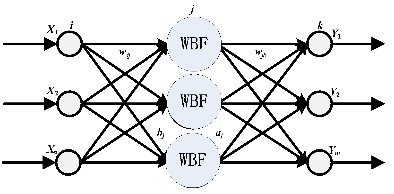
WNN is a kind of neural network based on BP neural network topology, using the Wavelet Basis Function (WBF) as the transfer function of the hidden layer nodes and the forward propagation of the signal while the error is propagated backwards [27]. Compared with the BP neural network, WNN has more sensitive approximation ability and stronger fault tolerance ability, better learning ability, and higher accuracy. The basic structure is shown in Figure 1.
2.2. Short Term Load Forecasting Using the WNN Model Based on MSD
This paper uses first-order difference and second-order difference for bad data identification. If the jth data point X(i, j) in the ith data is a dead pixel, the correction value X’(i, j) is as shown in Equation (1).
In order to make the forecasting model more adaptable, each MF data is normalized according to Equation (2).
where X is the original value. Y is the normalized value. Xmin and Xmax are the original minimum and maximum values respectively.
Then it calculates the correlation coefficient ζi(k) and the degree of correlation γi according to Equations (3) and (4).
As shown in Equation (5), it takes into account the degree of influence of each relevant influencing factor, calculates the weight αi of each relevant influencing factor through the degree of correlation, and uses the WSF to calculate the similitude of historical data on the ith day and the predicting date sim(k).
where θi is the weight of relevant influencing factors. zi(0) is the ith influencing factor of the forecasting day.
The short-term load forecasting process using the WNN model based on MSD is shown in Figure 2.
3. Short-Term Price Forecast Based on FC and GA-BP Neural Network
For short-term price forecasting, the BP neural network can realize complex highly nonlinear mapping, but it has slow convergence speed and low prediction accuracy [28,29,30]. In these papers, the FC analysis is used to select the learning samples to find out the prediction categories similar to the forecasting date as the input samples of the neural network. Also, the GA is used to optimize the BP neural network. So it not only conducts a broad mapping of neural networks and global search capabilities of genetic algorithm, but also speeds up the learning rate of the network.
3.1. FC Analysis Based on Transitive Closure
In order to effectively classify the samples, we must first distinguish the characteristic indicators of the sample itself. Assuming there are n samples and m characteristic indexes, we can construct a primitive matrix X of n × m, and xij represents the jth characteristic index of the ith sample. The historical price data and load data are normalized by Equation (2).
After the data normalization processing, in order to obtain a similar relationship between each sample or the degree of familiarity, the Fuzzy Similarity Matrix (FSM) needs to be calculated. The Euclidean distance method in the paper of M.A. Hakeem et al. [31]. was used to find the similarity between samples rij.
The FSM needs to be further processed by the transfer closure method to get the Fuzzy Equivalent Matrix (FEM). Suppose that X is a set of n samples to be classified, R is a FSM on X. Then there must be a minimum natural number k (k ≤ n), so that the transitive closure Rs* = Rsk, where the transitive closure is the FEM with the smallest distance from Rs and contains Rs, recorded as Re* [32]. In this paper, Re* is calculated by the square self-synthesis method, and Rs2 = Rs·Rs, Rs4 = Rs2·Rs2, …, Rs2k = Rsk·Rsk are calculated in turn until the value of k that satisfies the condition Re* = Rsk is the FEM.
According to the principle of clustering, it chooses the appropriate threshold γ to cut, then it can obtain the classification of the sample set. The best γ value can be obtained by adjusting Equation (7).
If Ci = max (Cj) exists, then the confidence level γi of the ith cluster can be considered as the optimal threshold.
3.2. Construction of GA-BP Neural Network Prediction Model
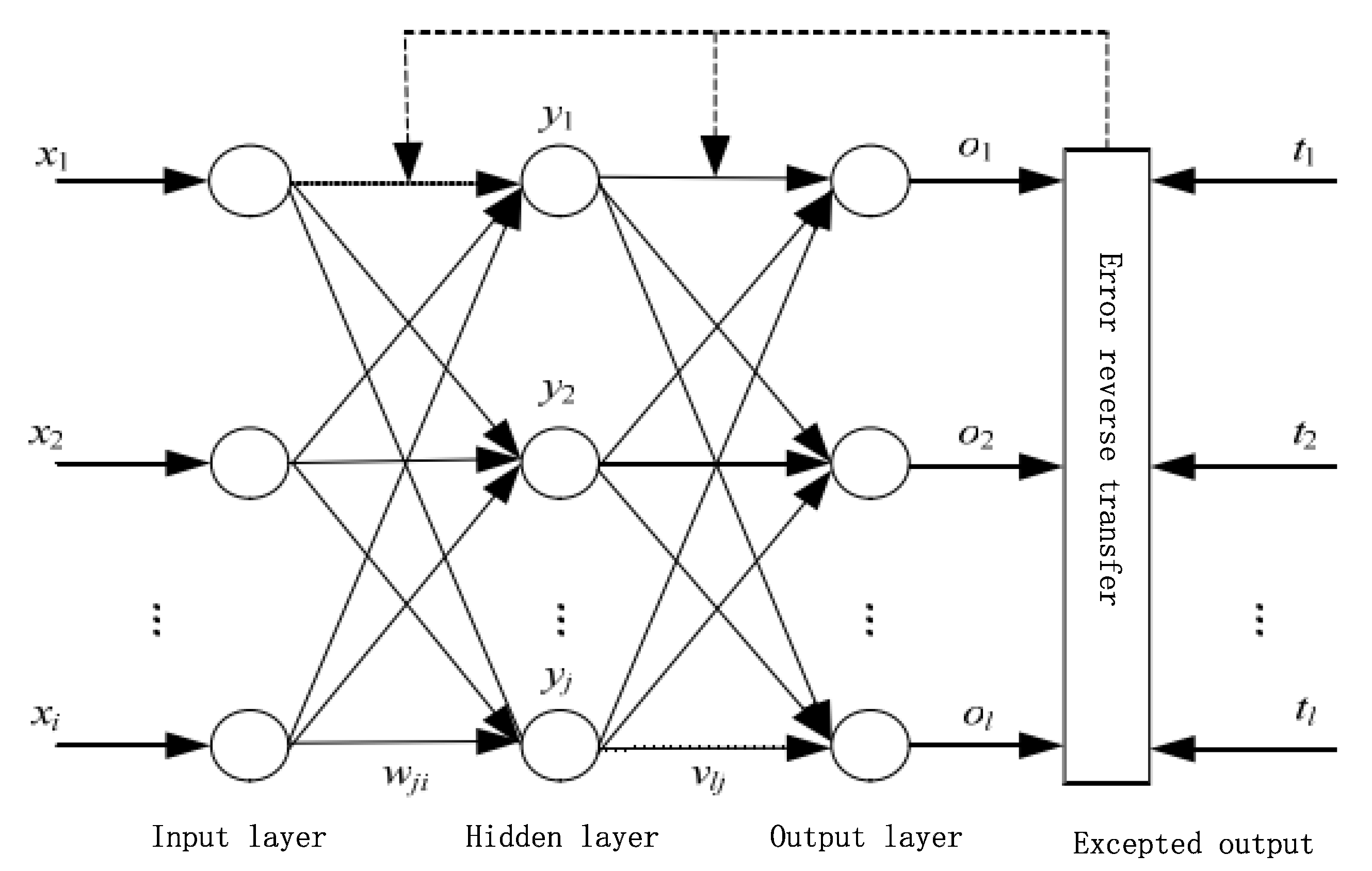
The BP neural network is a kind of multi-layer feed forward neural network which is trained according to the error back propagation algorithm and consists of input layer, hidden layer, and output layer. The BP neural network is the most used neural network by far, but it still has some drawbacks of slow convergence speed, long training time, and it is easy to make the objective function fall into local minima. A typical BP neural network structure model is shown in Figure 3.
The specific steps of GA for BP neural network optimization are as follows:
- (1)
- Determine the relevant parameters of GA and BP network, including population capacity of GA, crossover rate, mutation rate, structural parameters, and accuracy of BP network.
- (2)
- Generate a set of initialization weights and threshold distributions (chromosomes) randomly in the network, and encode each chromosome with a binary encoding to form an initial population.
- (3)
- Determine the fitness function through the network actual value and expected value of error function. Calculate fitness values for each individual and measure each chromosome. If the individual fitness meets the requirements, go to step (5), otherwise go to step (4).
- (4)
- GA optimizes network weight values and thresholds. Perform crossover and mutation operations at given probabilities to generate a new generation of individuals. Go to step (2) and enter the loop until the best populations and individuals are obtained.
- (5)
- Fine-tune with the BP neural network until the stop condition is satisfied.
- (6)
- The process of using the GA-BP neural network based on FC to predict short-term price is shown in Figure 4.
4. Bayesian Bidding Game Based on the SA
4.1. Day-Ahead Market Trade Considering Demand-Side Bidding
4.1.1. Power Trading Market Overview
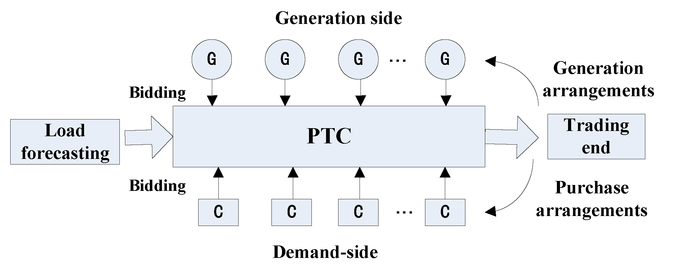
Electricity market trade can be divided into spot trade, contract trade, and futures trade according to the time and form of the transaction, while the spot trade includes day-ahead trade and real-time trade [33]. The day-ahead market is divided into 48 trading sessions, each trading session for 30 min. The day-ahead market is an important core of the electricity market, its market structure is shown in Figure 5.
4.1.2. Quotation Methods and Settlement Rules
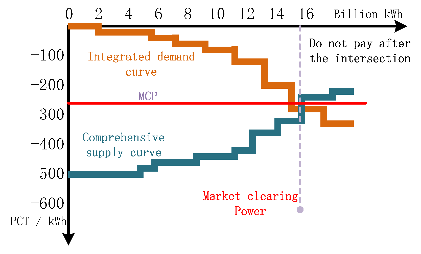
At present, the commonly used methods of quotation can be divided into time ladder quotation method and continuous quotation method. This article uses the sub-quotation method. Market participants can report up to K capacity segments for each trading session of the next day. The capacity value of each segment is called the segment capacity, and a price is declared for each capacity segment, which is called the segment price [34]. According to the requirements of the market rules, the quotations of Generation Companies (GenCos) should increase monotonically; that is, the prices of GenCos vary from low to high as the capacity segments increase. And the demand side submits several capacity segments according to the segment price ranges from high to low. The capacity segment submitted by each party in each period cannot exceed the maximum market requirement, that is, less than or equal to K. The Power Trading Center (PTC) will synthesize the corresponding supply curve and demand curve according to the quotations of each GenCo and demand side for each period respectively. After that, the PTC will determine the market clearing price and the bidding power of all parties according to the balance between supply and demand. The formation process of the MCP and clearing power are shown in Figure 6.
Currently, there are mainly two market settlement methods in the market: System Marginal Price (SMP) and Pay as Bid (PAB) [35]. The SMP is the most widely used method, its principle is to wait for quotation criteria; that is, the system clearing price is determined by the quotation of the last successful bidder in the system and as a uniform settlement price for the entire network. The market transaction type studied in this paper is day-ahead trade. Demand-side and GenCos make sub-quotations respectively. The PTC obtains the day-ahead MCP in accordance with the SMP method.
4.1.3. Day-Ahead Trading Patterns Considering the Demand-Side Bidding
With the continuous opening up of the demand side, the demand side response needs to be introduced in the market, and the co-competition between the demand side and the GenCos must be realized through the demand side bidding in the day-ahead market. The plan of a day-ahead trade scheme has generally been aimed at maximizing social welfare. Market participants declare their electricity and prices through a technical support system and take the form of bidirectional bidding; that is, the retailers declare the price difference with the price in the current list price, and GenCos declares the spread of the internet tariff. Power trading institutions consider safety constraints and make market clearing. After the checking of power dispatching agency safety, the final object of the transaction market, transaction volume and transaction price are determined. The demand side of the bidding electricity market trading day pattern is shown in Figure 7.
4.2. Bayesian Bidding Game Model Based on the SA
4.2.1. Sealed-Bid and Bayesian Nash Equilibrium
According to the game player’s access to information on the situation, the game can be divided into the complete information game and the incomplete information static game; that is, the Static Bayesian Game (SBG). Sealed-bid Auction in the paper of Bao, H. et al. refers to the bidders bidding each other with mutual understanding, submitting sealed bids and opening bids at the same time, and the highest bidder winning the auction [36]. Bayesian Nash Equilibrium in the paper of Zhang, F. et al. means that the expected utility of each game player is maximized when the probability distribution of own type and opponent type is known, which is the best of all the game parties strategy portfolios [37].
In the process of pursuing profit maximization, the retailer only knows its cost function and revenue function, and does not know the competitor’s relevant information, so it can be regarded as an incomplete game of static information. In this paper, the principle of SA is introduced, and SBG is used to study the optimal bidding strategy for the retailer.
4.2.2. Establishment of the Model
In order to simplify the study, this article considers only one period of the retailer’s bidding. This SBG problem can be described in a standard way as follows:
- (1)
- Behavioral space Ai: the retailer’s quotation Pi. Pi value is between the highest and the lowest price that is limited by the PTC, so the behavior space Ai = [f1, f2], (f1, f2 > 0).
- (2)
- Type space Ti: the cost of electricity sale of retailer Ci. It consists of operating costs and purchase costs, two parts. Assuming Cs ≤ Ci ≤ Ct, so the type space Ti = [Cs, Ct]. Competitors do not know the specific value of Ci, only through historical information do they estimate the probability to obtain it. Under the rule of market-clearing of electricity, this paper assumes that the operating cost ci* of the ith retailer is Equation (8), and Ci is Equation (9).
The sales function of the retailer is Equation (10).
where λi is the sales price of the retailer. ki is the response coefficient of the user to the sales price.
So the general profit function of the power retailer is Equation (11).
Assuming that the ith retailer’s quotation is a linear function of the cost of sales, the quotation function of the retailer i is Equation (12).
where Pi is the quotation of retailer i. αi, βi are quotation parameters.
4.3. Optimal Bidding Strategies under Different Probability Distributions
In the above, a mathematical method of probability is used to estimate the cost of the electricity sold of the opponent (other power company). Therefore, the retailer in the game analysis must make an accurate prediction of the probability distribution [36]. Different probability distributions will get different quotation results, thus affecting the bidding and profitability results.
According to the electricity market trading rules, the specific expression of the income function of the power retailer i is Equation (13).
where εQi denotes the amount of electricity that i succeeded in trading at last (0 < ε < 1). , represents the probability that the ratio of winning bid and bidding electricity of the retailer i is εm. means the probability that the quotation of retailer i is equal to the MCP.
The above three kinds of income are as follows:
- (1)
- The profit that the retailer’s quotation is higher than that of other competitors, and gain of all the bidding Qi.
- (2)
- The profit that the retailer’s quotes are the same as other competitors, and each retailer’s chance of winning the bid is 1/n.
- (3)
- The profit that the retailer’s quotes are lower than other competitors, it purchases part of the bidding power.
When the retailer’s quote is lower than the R value, it must have a power of 0 and a return of 0.
Assuming that the cost of sales electricity Ci obeys the uniform distribution (UD) on [cs, ct], it can be seen that the quotation Pi (Ci) obeys the UD on [−βi cs + αi, −βi ct + αi]. Therefore, in the case of continuous distribution, the probability that different retailers have same quote is zero, that is, P (Pi = Pj) = 0. Suppose the BNE is [Pi, Pj] (I ≠ j) when the profit of retailer is maximized, that is, for each Ci∈Ti, Pi (Ci) satisfies Equation (14).
Since both Ci and Cj obey the UD on [cs, ct], so we can get Equation (15).
At this point equation, Equation (14) can be rewritten as Equation (16).
According to the Lagrange theorem, for obtaining the optimal solution, the objective function needs to be derived and the partial derivative and the derivative value should be zero.
Combined with Equation (9) one can further obtain Equation (18) of the quotation Pi.
From the expression of the optimal bidding of power retailer, it can be seen that the optimal bidding of the retailer is related to the selling cost (parameter), selling price, MCP, purchasing power, and cost distribution interval.
When Ci obeys the normal distribution with distribution density (ND) [μ, σ2], that is Ci~N (μ, σ2), so Pi (Ci)~N (−βiμ + αi, (αiσ)2). Therefore, in the case of continuous distribution, the probability that different retailers have the same quote is zero, so the objective function is still Equation (14). However, the distribution density function becomes complicated at this time. In the process of solving Equation (14) to get the optimal quote Pi*, using the manual derivation method is very cumbersome and even may not be solved. The methods commonly used to solve unconstrained optimization problems are Newton’s method, the conjugate gradient method, and the variable metric method (also called DFP method) [38]. The DFP algorithm not only retains the advantages of Newton’s fast convergence speed, but also reduces the complexity of the second-order derivative operation, and has less memory requirements. Therefore, this paper uses the DFP algorithm, programming with MATLAB to solve the most optimal quote Pi* which makes the objective function maximized.
The basic idea of the DFP method is to generate a positive definite symmetric matrix Hk+1 at every iteration point Xk+1 according to a certain rule, and then use Pk+1 = −Hk+1 gk+1 as the searching direction at Xk+1 (gk+1 is the gradient of the objective function at the iteration point Xk+1) [36].
If the gk+1 ≠ 0, the Pk+1 is the descending direction.
Since Pi and Pj obey the ND in interval [Ps, Pt], so P (Pi <Pj) = 1 − P (Pi >Pj), and then one can get the objective function by solving Equation (20).
5. Case Study
This article selects historical electricity price data from the PJM market in the United States from 28 August 2016 to 15 October 2016 (one sampling point every 30 min, daily 48 points, dimension $), historical electricity load data from 1 January 2010 to 15 October 2016 (one sampling point every 15 min, daily 96 points, dimension MW) and meteorological data from 1 January 2013 to 22 October 2016 (daily maximum temperature, daily minimum temperature, daily average temperature, daily relative humidity, and daily rainfall) as samples; using MATLAB (2014a, MathWorks, Natick, MA, USA) data software to implement the load forecasting and clearing price forecasting and then obtaining the BNE under different probability distributions.
5.1. Short-Term Load Forecasting
Load forecasting of users in retailers’ respective regions is very important for them to make electricity purchase. Accurate load forecasting can avoid surplus or shortage of electricity and directly affect the final revenue of the retailer. According to the prediction method mentioned above, the given data are processed and predicted, and the load values with or without the impact of MF are obtained from 16 to 22 October 2016. To analyze the prediction accuracy, one compares the load forecasting curve with the forecast input average, and the corresponding curve is shown in Figure 8.
As can be seen from Figure 8, the prediction curves that considered and did not consider MF are basically consistent. However, some details of the curve (for example, from period 1 to period 100 and period from 300 to 400 in Figure 8) show that when the MF is taken into consideration, the prediction curve will be closer to the average value of the predicted input. To a certain extent, this shows that the forecasting curve counting MF is more accurate.
In order to more rigorously demonstrate the accuracy of the forecasting curve taking MF into consideration, the mean absolute percentage error (MAPE) for each case can be calculated. As can be seen from Table 1, the MAPE values counting MF are smaller than those not counted. Therefore, it has been proved that considering the MF can improve the short-term load forecasting accuracy to a certain extent.
5.2. Short-Term Price Forecasting
First, select the input samples for FC. The sample set is constructed based on the raw electricity price, and each sample contains 14 characteristic indexes, which are the same forecast point price, the same forecast point load, the number of market participants, the generation fuel cost, and the weather type value on 14–16 October, respectively. Then use fuzzy clustering to analyze the cluster. Based on the similarities of the comprehensive indexes, 12 categories similar to the 16th (the shortest European distance) are selected as the input samples of the neural network.
Secondly, determine the GA-BP neural network parameters. Take the number of nodes in the input layer of neural network as 14, and the number of neurons in the hidden layer as 12, which is equal to the number of input samples and the number of output as 1. So the structure of the neural network can be obtained as 14-12-1. In order to prevent the cycle of death, the maximum number of iterations selected here is 3000, the crossover probability Pc is 0.9, the mutation probability Pm is 0.001 [39,40,41].
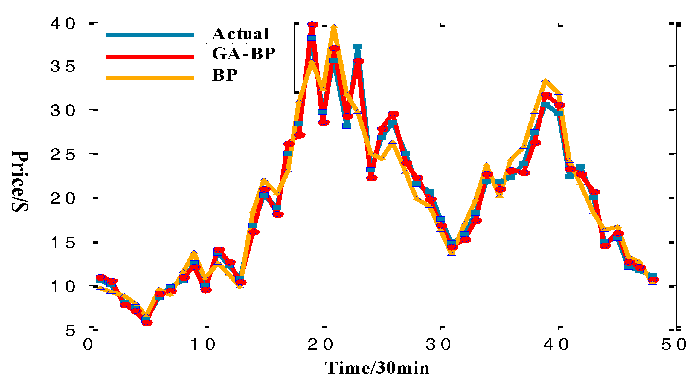
Finally, implement the real-time electricity price forecast on 48 periods of 16 October according to the method described above. The comparison of the GA-BP neural network prediction value, BP neural network prediction value, and real value is shown in Figure 9.
It can be seen from the calculation results and the comparison chart that the peak period of electricity price is between 18 and 25 h and from 38 to 42 h, because the electricity load is larger and the demand is higher at this time. In the early morning, the electricity load is small, so the electricity price is in the trough area. The MAPE between the predicted value and the true value of GA-BP neural network is 3.42%–4.45%, and the MAPE between the predicted value of BP neural network and the real value is 7.76%–10.12%. It shows that the method proposed in this paper can predict price more accurately and provide more accurate guidance for power retailers.
In order to facilitate the analysis of the problem and make the result more clear, this article makes the following assumptions:
- (1)
- This article only studies the auction situation in one period (other periods can be analogized).
- (2)
- There is no blocking phenomenon in the network, that is, the network structure does not affect the clearing result.
- (3)
- In the example described, there are five retailers in the electricity market to compete, the relevant parameters of retailers are shown in Table 2, where the operating cost parameter ci = 0 (i = 1, 2, 3, 4, 5). Qi is the integer value after rounding the retailers’ load forecast value. Ri is the MCP forecast value of retailers at this time. The real MCP is 20.38$.
- (4)
- The market can supply electricity to 100 MW.
5.2.1. The Impact of Different Probability Distributions on Quotation
Suppose that the cost of electricity sales Ci (i = 1, 2, 3, 4, 5) is uniformly distributed over the interval [18,22]. Equation (18) will calculate d by a simple calculation program written in MATLAB. In this process, when the BNE value of the retailer i is less than the predicted MCP value, the predicted MCP value is the final quotation of i. Table 3 shows the retailers’ final bidding strategies which include purchased power, quotes and revenue.
As can be seen from Table 3, when there is no network constraint, if all retailers are bidding according to the optimal strategy of Table 3, the PTC hires these quotes from high to low, so retailer 1, retailer 4, and retailer 5 obtained all the required power, retailer 3 bought the remaining power in the market, and retailer 2 was not selected because of the lowest quote. However, due to the inaccurate estimation of the distribution of the electricity price, the quote of retailer 4 is higher than the price of its sales, which has a risk of loss.
Assuming that the sales cost Ci (i = 1, 2, 3, 4, 5) of a retailer is subject to ND with distribution density of [0.3, 2]. The DFP algorithm programming written by MATLAB is used to solve Equation (20). When each retailer reaches the BNE, combined with their predicted MCP, the final purchase quantity, quotation and its own revenue results are obtained and listed in Table 4.
As can be seen, when there is no network constraint, if all retailers are bidding according to the optimal strategy of Table 4, the PTC hires these quotes from high to low, so retailer 1, retailer 2, and retailer 4 obtained all the required power. As the BNE value was lower than the predicted MCP value, retailer 3 and retailer 5 all took the predicted value as the final quotation result and divided the remaining power by average. Retailer 4 was in a profitable state. This shows the importance of accurate estimation of the distribution of electricity prices during the game analysis. The MAPE values for the final quotes and the MCP of two distributions are all shown in Table 5.
From the above analysis, we can see that the accurate estimate of electricity price probability distribution not only helps to predict the trend of short-term market behavior, but also helps the power retailer form an effective and dominant bidding strategy. Comparison of the uniform distribution price (UDP), normal distribution price (NDP) and real MCP of each retailer in the same period of time can be seen in the histogram in Figure 10.
5.2.2. Impact of Short-Term Price Forecasting on the Bidding Strategy of the Power Retailer
Table 4 above shows the optimal bidding strategy combination obtained after implementing load forecasting and MCP forecasting in a period of time when five retailers considered that their opponents’ quotes obeyed ND. However, if the retailer does not forecast the MCP, the BGM will be directly solved for the final quote only after the expected electricity purchase volume is determined by the load forecast, and the result of the quotation and the actual purchased volume will change. The comparison of the final purchase power in both cases and the expected purchase power are shown in Figure 11.
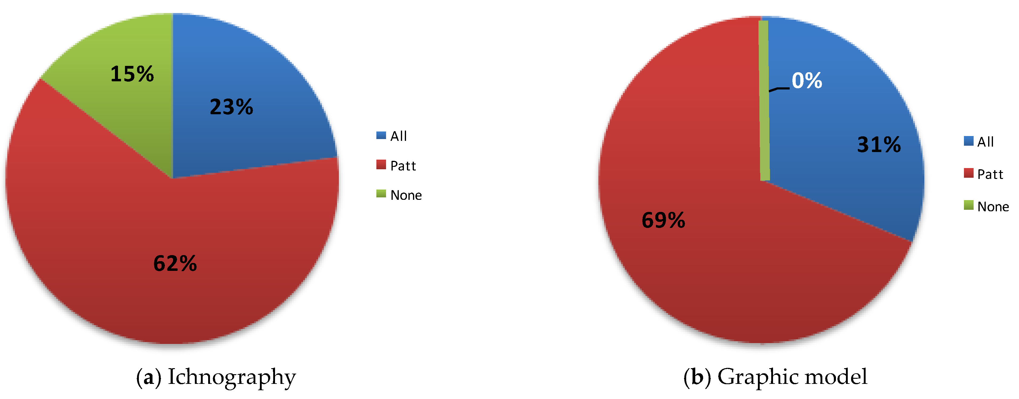
Since retailer 5 is more representative, conducting further research on both cases of retailer 5 implements price forecasting but does not implement price forecasting in the 48 h of the day. Also, one needs to divide the 48 periods of power purchase situation into “buy all electricity” (named “All” in Figure 12), “buy part of the electricity” (named “Part” in Figure 12) and “non-purchased electricity” (named “None” in Figure 12) third gear statistics. The pie chart is shown in Figure 12.
It can be seen from the comparison that in the 48 h of the whole day, the probability that retailer 5 fails to purchase power after performing the MCP prediction at each time period is 0, and the proportions of the time when all or part of the expected power is purchased are all larger than that when the MCP is not predicted. Therefore, it is very important to forecast the short-term electricity price when formulating the optimal bidding strategy for the power retailer.
6. Conclusions
Aiming at the optimal bidding strategy of the power retailer which was researched in this paper, we obtain the following conclusions through modelling, solution, and analysis:
In order to guide the retailer to make purchase of electricity better, this paper introduced the concept of MSD, selecting the load value of similar days as part of the training and forecasting of the WNN. From the result analysis, it can be seen that the WNN prediction model based on the meteorological similarity day proposed in this paper can improve the prediction accuracy to a certain extent.
In order to provide a reference for the retailer, this paper established a GA-BP neural network prediction model based on FC to predict the short-term MCP. The results show that the clustering of samples based on a variety of factors affecting the price of electricity, and the use of GA to optimize the weight of the BP network improve the prediction accuracy to a certain extent.
The bidding of the power retailer can be regarded as a game problem with incomplete information. Based on the SA model in game theory, this paper proposed a bidding BGM based on the SA, and obtained a better BNE solution meeting the requirements. The example showed that different probability density distributions of adversary quotes affect their own quotations. Combined with the forecast of the short-term MCP, this could guide the retailers to improve their bidding to gain the maximum benefits.
Acknowledgments
This work was supported in part by the Nature Science Foundation of China (51607068), and the Fundamental Research Funds for the Central Universities (2018MS082).
Author Contributions
The author Xiaojie Zhou carried out the main research tasks and wrote the full manuscript, and Yajing Gao proposed the original idea, analyzed and double-checked the results and the whole manuscript. Jiafeng Ren contributed to data processing and to writing and summarizing the proposed ideas, while Zheng Zhao provided technical and financial support throughout. Fushen Xue provided guidance and assistance in model modification during the revision of the paper.
Conflicts of Interest
The authors declare no conflict of interest.
Abbreviations
The following abbreviations are used in this manuscript:
| WNN | Wavelet neural network |
| MSD | Meteorological similarity day |
| GA | Genetic algorithm |
| BP | Back propagation |
| FC | Fuzzy clustering |
| SA | Sealed-bid auction |
| BGM | Bayesian game model |
| BNE | Bayesian Nash equilibrium |
| EEX | European energy exchange |
| PJM | Pennsylvania New Jersey Maryland |
| ISO | Independent system operation |
| EPF | Electricity price forecasting |
| CNN | cascade neural network |
| FEEMD | Fast ensemble empirical mode Decomposition |
| VMD | Variation mode decomposition |
| SFE | Supply Function Equilibrium-based |
| MF | Meteorological factors |
| GRA | Gray relational analysis |
| WSF | Weighted similarity formula |
| WBF | Wavelet basis function |
| FSM | Fuzzy similarity matrix |
| FEM | Fuzzy equivalent matrix |
| GenCos | Generation companies |
| PTC | Power trading center |
| SMP | System marginal price |
| PAB | Pay as bid |
| SBG | Static Bayesian game |
| UD | Uniform distribution |
| ND | Normal distribution |
| MAPE | Mean absolute percentage error |
| UDP | Uniform distribution price |
| NDP | Normal distribution price |
References
- Meyabadi, A.F.; Deihimi, M.H. A review of demand-side management: Reconsidering theoretical framework. Renew. Sustain. Energy Rev. 2017, 80, 367–379. [Google Scholar] [CrossRef]
- Li, W.; Xu, P.; Lu, X.; Wang, H.; Pang, Z. Electricity demand response in China: Status, feasible market schemes and pilots. Energy 2016, 114, 981–994. [Google Scholar] [CrossRef]
- Wen, B.; Zhou, F.; Cheng, H.Z.; Yu, J.; Gao, G.M. A Review of Auxiliary Services and Pricing in Electricity Market. East China Power 2001, 11, 30–34. [Google Scholar]
- The Country Has Publicized 1371 Sales Companies. 2017. Available online: http://shoudian.bjx.com.cn/news/20170413/819998.shtml (accessed on 13 April 2017).
- Vilar, J.; Aneiros, G.; Raña, P. Prediction intervals for electricity demand and price using functional data. Int. J. Electr. Power Energy Syst. 2018, 96, 457–472. [Google Scholar] [CrossRef]
- Zhang, P.; Pan, X.P.; Xue, W.C. Prediction of short-term load based on wavelet decomposition fuzzy gray clustering and BP neural network. Electr. Power Autom. Equip. 2012, 32, 121–125. [Google Scholar]
- Ak, R.; Li, Y.F.; Vitelli, V.; Zio, E. Adequacy assessment of a wind-integrated system using neural network-based interval predictions of wind power generation and load. Int. J. Electr. Power Energy Syst. 2018, 95, 213–226. [Google Scholar] [CrossRef]
- Wang, B.Y.; Zhao, S.; Zhang, S.M. Distributed Electric Load Forecasting Algorithm Based on Cloud Computing and Extreme Learning Machine. Power Syst. Technol. 2014, 38, 526–531. [Google Scholar]
- Bessec, M.; Fouquau, J. Short-run electricity load forecasting with combinations of stationary wavelet transforms. Eur. J. Oper. Res. 2018, 264, 149–164. [Google Scholar] [CrossRef]
- Weron, R. Electricity price forecasting: A review of the state-of-the-art with a look into the future. Int. J. Forecast. 2014, 30, 1030–1081. [Google Scholar] [CrossRef]
- Silvano, C.; Giulia, G.; Linda, P.; Marco, R. Modeling and forecasting of electricity spot-prices: Computational intelligence vs classical econometrics. AI Commun. 2014, 27, 301–314. [Google Scholar]
- Nima, A.; Keynia, F. Day ahead price forecasting of electricity markets by a mixed data model and hybrid forecast method. Int. J. Electr. Power Energy Syst. 2008, 30, 533–546. [Google Scholar]
- Deng, J.J.; Huang, Y.S.; Song, G.F. Application of non-parametric GARCH-based time series model to forecasting electricity prices in the near future. Power Syst. Technol. 2012, 36, 190–196. [Google Scholar]
- Bento, P.M.R.; Pombo, J.A.N.; Calado, M.R.A.; Mariano, S.J.P.S. A bat optimized neural network and wavelet transform approach for short-term price forecasting. Appl. Energy 2018, 210, 88–97. [Google Scholar] [CrossRef]
- Shi, B.; LI, Y.; Yu, X.; Yan, W.; Li, N.; Meng, X. Short-Term Electricity Price Forecast Model Based on Adaptive Variable Coefficients Particle Swarm Optimizer and Radial Basis Function Neural Network Hybrid Algorithm. Power Syst. Technol. 2010, 34, 98–106. [Google Scholar]
- Yan, X.; Chowdhury, N.A. Mid-term electricity market clearing price forecasting: A multiple SVM approach. Int. J. Electr. Power Energy Syst. 2014, 58, 206–214. [Google Scholar] [CrossRef]
- Wang, D.; Luo, H.; Grunder, O.; Lin, Y.; Guo, H. Multi-step ahead electricity price forecasting using a hybrid model based on two-layer decomposition technique and BP neural network optimized by firefly algorithm. Appl. Energy 2017, 190, 390–407. [Google Scholar] [CrossRef]
- Hong, Y.Y.; Liu, C.Y.; Chen, S.J.; Huang, W.C.; Yu, T.H. Short-term LMP forecasting using an artificial neural network incorporating empirical mode decomposition. Int. Trans. Electr. Energy Syst. 2015, 25, 1952–1964. [Google Scholar] [CrossRef]
- Gabriel, S.A.; Kiet, S.; Balakrishnan, S. A mixed integer stochastic optimization model for settlement risk in retail electric ower markets. Netw. Spat. Econ. 2004, 4, 323–345. [Google Scholar] [CrossRef]
- Bartelj, L.; Gubina, A.; Paravan, D.; Golob, R. Risk management in the retail electricity market: The retailer’s perspective. In Proceedings of the IEEE Power and Energy Society General Meeting, Providence, RI, USA, 25–29 July 2010; pp. 1–6. [Google Scholar]
- Anderson, E.J.; Philpott, A.B. Optimal Offer Construction in Electricity Markets. Math. Oper. Res. 2002, 27, 82–100. [Google Scholar] [CrossRef]
- Fleten, S.E.; Pettersen, E. Constructing bidding curves for a price-taking retailer in the Norwegian electricity market. IEEE Trans. Power Syst. 2005, 20, 701–708. [Google Scholar] [CrossRef]
- Nassiri-Mofakham, F.; Nematbakhsh, M.A.; Baraani-Dastjerdi, A.; Ghasem-Aghaee, N.; Kowalczyk, R. Bidding strategy for agents in multi-attribute combinatorial double auction. Expert Syst. Appl. 2015, 42, 3268–3295. [Google Scholar] [CrossRef]
- Hematabadi, A.A.; Foroud, A.A. A new solution approach to supply function equilibrium-based bidding strategy in electricity markets. Sci. Iran. Trans. D Comput. Sci. Eng. Electr. 2017, 24, 3231–3246. [Google Scholar] [CrossRef]
- Dai, Y.M.; Gao, Y. Multi-retailer Real-time Pricing Strategy Based on Demand Side Management of Smart Grid. Proc. CSEE 2014, 34, 4244–4249. [Google Scholar]
- Gao, Y.J.; Sun, Y.J.; Yang, W.H.; Chuo, B.; Liang, H.F.; Li, P. Short-term prediction of meteorological sensitive load based on new type of human comfort. Chin. J. Electr. Eng. 2017, 37, 1946–1955. [Google Scholar]
- Androvitsaneas, V.P.; Alexandridis, A.K.; Gonos, I.F.; Dounias, G.D.; Stathopulos, I.A. Wavelet neural network methodology for ground resistance forecasting. Electr. Power Syst. Res. 2016, 140, 288–295. [Google Scholar] [CrossRef]
- Hakeem, M.A.; Kamil, M. Analysis of artificial neural network in prediction of circulation rate for a natural circulation vertical thermosiphon reboiler. Appl. Therm. Eng. 2017, 112, 1057–1069. [Google Scholar] [CrossRef]
- Xiao, B.; Liu, Q.Y.; Niu, Q.; Xu, X.S.; Wang, H. Spatial Load Forecasting Based on RBF Neural Network Based on Cell Load Characterization. Power Syst. Technol. 2018, 42, 301–307. [Google Scholar]
- Fei, W.; Zhong, D.W.; Qiang, L. Short-term Wind Energy Prediction Algorithm Based on SAGA-DBNs. DEStech Trans. Comput. Sci. Eng. 2016. [Google Scholar] [CrossRef]
- Zu, X.R.; Tian, M.; Bai, Y. A short-term load forecasting method based on fuzzy clustering and wavelet kernel regression. Electr. Power Autom. Equip. 2016, 36, 134–140. [Google Scholar]
- Yao, L.X.; Song, L.F.; Li, Q.Y.; Wan, S.X. Prediction of short-term load in power system based on fuzzy clustering analysis and BP neural network. Power Syst. Technol. 2005, 1, 20–23. [Google Scholar]
- Bao, H.; Ai, D.P.; Yang, Y.H.; Wu, W. Global power generation trading model combined with long-term and recent market. Power Syst. Technol. 2012, 36, 264–270. [Google Scholar]
- Zhang, F.; Bao, H.; Yang, Y.H.; Yang, X.Y. Trading market bidding model considering network loss correction. Power Syst. Technol. 2011, 35, 164–169. [Google Scholar]
- Zeng, L.; Qi, H.; Chen, Y.C. Power bidding strategy for multi-objective bidding of generation companies in real-time and real-time markets. Power Syst. Technol. 2009, 33, 65–70. [Google Scholar]
- Zhou, X.J.; Gao, Y.; Yang, W.; Guo, W. Bidding strategy of electricity market considering network constraint in new electricity improvement environment. J. Eng. 2017, 13, 1640–1645. [Google Scholar] [CrossRef]
- Yu, S.; Wang, K.; Wei, Y.M. A hybrid self-adaptive Particle Swarm Optimization–Genetic Algorithm–Radial Basis Function model for annual electricity demand prediction. Energy Convers. Manag. 2015, 91, 176–185. [Google Scholar] [CrossRef]
- Liu, Y.X.; Guo, L.; Wang, C.S. A bidding game approach for power distribution market with multi-microgrid. Power Syst. Technol. 2017, 41, 2469–2476. [Google Scholar]
- Gong, E.L.; Duan, L.N.; Gao, M.M.; Wang, Z.Z.; Zhu, M.Y.; Sun, Q.Y.; Du, X.Y. A two-stage non-monotone sparse diagonal scaling scaling gradient projection algorithm based on modified quasi-Newton equation. Math. Pract. Underst. 2017, 47, 233–242. [Google Scholar]
- Liu, L.L.; Wang, Q.F.; Lin, H.B. Parameters Setting and Application of BP Neural Network. Optim. Cap. Constr. 2007, 28, 101–106. [Google Scholar]
- Li, A.X.; Chen, J. A Review of BP Neural Network Parameter Improvement Methods. Electron. Sci. Technol. 2007, 2, 79–82. [Google Scholar]
Figure 1.
Wavelet neural network (WNN) structure diagram.

Figure 2.
Short-term load forecasting flow chart using WNN based on the meteorological similarity day (MSD).
Figure 2.
Short-term load forecasting flow chart using WNN based on the meteorological similarity day (MSD).

Figure 3.
BP neural network structure diagram.

Figure 4.
GA-BP neural network prediction flow chart based on fuzzy clustering (FC)

Figure 5.
Day-ahead trade structure chart.

Figure 6.
The formations of MCP and clearing power.

Figure 7.
Day-ahead trade pattern considering the demand-side bidding.

Figure 8.
Contrast diagram of the predicted value and the predictive input mean value with or without the impact of meteorological factors.
Figure 8.
Contrast diagram of the predicted value and the predictive input mean value with or without the impact of meteorological factors.

Figure 9.
The 48-period GA-BP, BP prediction and real-value comparison chart.

Figure 10.
Contrast diagram of the power retailers’ UDP, NDP, and MCP.

Figure 11.
Contrast diagram of final purchase power in both cases and expected purchase power.

Figure 12.
Diagram of the graded purchased power situation of retailer 5.


Table 1.
Prediction accuracy comparison of counting or not counting meteorological factors (MF).
| Date | 16th | 17th | 18th | 19th | 20th | 21th | 22th | |
|---|---|---|---|---|---|---|---|---|
| MAPE (%) | Not Counting MF | 5.28 | 1.17 | 0.49 | 1.74 | 3.55 | 2.59 | 1.27 |
| Counting MF | 5.18 | 1.14 | 0.45 | 1.60 | 3.53 | 2.57 | 1.17 |
Table 2.
Power retailer parameters.
| Power Retailer | ai | bi | ki | λi/$ | Qi/MW | Ri/$ | |
|---|---|---|---|---|---|---|---|
| 1 | 0.0235 | 0.065 | 0.041 | 22.78 | 30 | 21.26 | |
| 2 | 0.0235 | 0.050 | 0.032 | 22.13 | 25 | 20.38 | |
| 3 | 0.0357 | 0.075 | 0.036 | 22.81 | 30 | 20.38 | |
| 4 | 0.0345 | 0.065 | 0.045 | 23.07 | 15 | 20.38 | |
| 5 | 0.0375 | 0.085 | 0.036 | 22.94 | 30 | 20.38 | |
Table 3.
Power retailers’ bidding strategies.
| Power Retailer | Purchased Power/MW | Pi/$ | Revenue/$ |
|---|---|---|---|
| 1 | 30 | 22.481 | 27.62394 |
| 2 | 0 | 22.006 | 0 |
| 3 | 25 | 22.216 | 17.83184 |
| 4 | 15 | 23.506 | 7.662379 |
| 5 | 30 | 22.697 | 21.55523 |
Table 4.
Power retailers’ bidding strategies.
| Power Retailer | Purchased Power/MW | BNE Value | Pi/$ | Revenue/$ |
|---|---|---|---|---|
| 1 | 30 | 22.206 | 22.206 | 27.62394 |
| 2 | 25 | 21.532 | 21.532 | 12.14092 |
| 3 | 15 | 21.158 | 21.26 | 8.56184 |
| 4 | 15 | 22.447 | 22.447 | 7.662379 |
| 5 | 15 | 21.047 | 21.26 | 9.74273 |
Table 5.
The MAPE of power retailers’ final quotations and MCP.
| Power Retailer | 1 | 2 | 3 | 4 | 5 | |
|---|---|---|---|---|---|---|
| MAPE (%) | UD | 10.31 | 7.98 | 9.01 | 15.34 | 11.37 |
| ND | 8.99 | 5.65 | 3.82 | 10.14 | 3.27 | |
© 2018 by the authors. Licensee MDPI, Basel, Switzerland. This article is an open access article distributed under the terms and conditions of the Creative Commons Attribution (CC BY) license (http://creativecommons.org/licenses/by/4.0/).
Share and Cite
MDPI and ACS Style
Gao, Y.; Zhou, X.; Ren, J.; Zhao, Z.; Xue, F. Electricity Purchase Optimization Decision Based on Data Mining and Bayesian Game. Energies 2018, 11, 1063. https://doi.org/10.3390/en11051063
AMA Style
Gao Y, Zhou X, Ren J, Zhao Z, Xue F. Electricity Purchase Optimization Decision Based on Data Mining and Bayesian Game. Energies. 2018; 11(5):1063. https://doi.org/10.3390/en11051063
Chicago/Turabian StyleGao, Yajing, Xiaojie Zhou, Jiafeng Ren, Zheng Zhao, and Fushen Xue. 2018. "Electricity Purchase Optimization Decision Based on Data Mining and Bayesian Game" Energies 11, no. 5: 1063. https://doi.org/10.3390/en11051063
Note that from the first issue of 2016, this journal uses article numbers instead of page numbers. See further details here.