Predicting Charging Time of Battery Electric Vehicles Based on Regression and Time-Series Methods: A Case Study of Beijing

Abstract

Battery electric vehicles (BEVs) reduce energy consumption and air pollution as compared with conventional vehicles. However, the limited driving range and potential long charging time of BEVs create new problems. Accurate charging time prediction of BEVs helps drivers determine travel plans and alleviate their range anxiety during trips. This study proposed a combined model for charging time prediction based on regression and time-series methods according to the actual data from BEVs operating in Beijing, China. After data analysis, a regression model was established by considering the charged amount for charging time prediction. Furthermore, a time-series method was adopted to calibrate the regression model, which significantly improved the fitting accuracy of the model. The parameters of the model were determined by using the actual data. Verification results confirmed the accuracy of the model and showed that the model errors were small. The proposed model can accurately depict the charging time characteristics of BEVs in Beijing.

1. Introduction

With the rapid development of the global automobile industry, the increasing vehicle ownership has resulted in worsening problems of environmental pollution and energy shortage. Battery electric vehicles (BEVs) have become a mainstream technology direction that promotes energy conservation, emission reduction and environmental protection due to their good environmental protection and energy adjustment effects. They have an unparalleled advantage over conventionally fueled vehicles to realise the automobile industry’s technological transformation, upgrading and development [1]. However, BEVs have the disadvantage of short driving range compared to conventional fuel vehicles. Therefore, BEV drivers need to charge their vehicles during trips [2]. Charging processes take a long time, so the charging behaviour during trips prolongs the driver travel times [3]. These problems pose a serious obstacle for drivers in choosing BEVs to travel. The accurate prediction of charging time can effectively alleviate the inconvenience to drivers caused by the inevitable charging behaviour during trips. Drivers can predict the charging time in advance according to the state of the vehicle to plan for efficient travel. Therefore, attention should be given to the charging time prediction in the charging behaviour of BEV drivers.

Charging time accounts for a relatively large proportion in the total travel time, which is an important factor for charging behaviour [4]. Recently, few studies on the problem of charging time prediction for BEVs have been conducted. In practice, accurately predicting charging time is difficult because environmental and other unobservable factors can affect the charging time of BEVs. With the recent development of data collection techniques, large volumes of data for BEV charging events can be obtained. Besides the observable factors, many environmental and unobservable factors are hidden in the data. Establishing a model through the data is an effective method to realize the accurate charging time prediction.

In this study, a prediction model of BEV charging time was built based on charge and discharge data that were collected from 70 BEVs in Beijing, China. The data were representative because the BEVs used to collect data operate like other vehicles in the road network and the charging behaviour in real-world condition can be reflected in the data. Notably, compared with the data used in previous literature, the data used in this study to fit the prediction model of charging time were collected from BEVs in Beijing. The data used in the previous studies were mainly collected from BEVs in the USA. The traffic and charging environment in other countries and areas, such as China, differ from those in the USA. For example, most BEV drivers in the USA charge their vehicles by using private chargers at home. However, in China, private chargers are not widely installed at residences due to the constrained residential and traffic conditions. Public charging stations are the main mode used to charge BEVs in China. This finding indicates that the characteristic of charging behaviour in the USA and China is different. Therefore, most of the previous research results on charging behaviour are not suitable for the condition in Beijing. The proposed model is suitable to be applied in predicting charging time of BEVs in Beijing and other similar areas. Moreover, in real-world scenarios, the charging time of BEVs is affected by several factors, such as battery capacity, residual energy, battery health state, battery charging efficiency and charged amount. Some factors cannot be directly observed, such as battery health state and battery charging efficiency, and thus cannot be used to build a prediction model of charging time. However, the unobservable factors have significant impacts on the charging time of BEVs. Therefore, the charging time prediction model without the unobservable factors leads to a significant prediction error. To address the problem, a time-series method was used to fit the prediction error that results from the unobservable factors, thereby reducing the prediction error and improving the prediction accuracy. A combined model for charging time prediction, which simultaneously adopts the regression and time-series methods for modelling, was established based on the actual data. The proposed model may be used by BEV drivers to determine their travel plan or by city planners to design public charging infrastructure considering the charging behaviour of BEV drivers.

The rest of the paper is organised as follows: in Section 2, the literature review is presented. In Section 3, the data sources are described and the data processing is introduced. In Section 4, a combined model for predicting charging time of BEVs is built based on the regression and time-series methods by using the actual data. In Section 5, the conclusions and directions for future research are presented.

2. Literature Review

Charging time is one of the most important factors for charging behaviour. It has a significant impact on the travel time of BEVs. However, few studies have explored the charging time and its prediction. In recent years, several studies have explored the charging behaviour and its impacts from the perspective of a power grid system operation, because the charging behavior of BEV drivers has significant impacts on power grid systems. He et al. [5] established the dynamic models for the BEV battery and power systems, and the impacts of the charging behaviour of BEV drivers on the power systems were explored based on the dynamic models. Clement-Nyns et al. [6] discussed the impacts of charging behavior on a residential distribution grid. A coordinated charging strategy was proposed to minimize the power losses and to maximize the main grid load factor. An et al. [7] proposed a computational framework for decision-making process of charging behaviour. The vehicle-to-grid services were considered in the framework, which aimed to improve the operational efficiency and security of power grid systems. Habib et al. [8] analysed the impacts of various conditions of charging behaviour on power grid systems. The coordinated/un-coordinated charging, delayed charging and off-peak charging were analysed to explore their impacts on power grid systems. Zhang et al. [9] proposed a decentralized BEV charging strategy to ensure high-efficiency charging and reduce load variations for power grid systems during charging periods. An extensive set of simulations and case studies with real-world data were used to demonstrate the benefits of the proposed strategies and the impacts of proposed charging strategy on power grid systems were discussed. Cui et al. [10] established a multi agent-based simulation framework to model the spatial distribution of BEV ownership at local residential level. Based on the framework, the impacts of the charging behavior resulting from the increasing BEV ownership on the local power grid system were explored by considering different charging strategies.

Moreover, related to the charging behaviour of BEVs, there are several studies that have discussed the methods to mitigate the concentrated charging. Kumar and Tseng [11] examined the impacts of demand response management on the chargeability of BEVs and proposed a scheduling driven algorithm to mitigate the concentrated charging. Aziz et al. [12] developed a battery-assisted charging system to improve the charging performance of a quick charger for BEVs. In addition, the effects of proposed system on mitigating the concentrated charging in different seasons were demonstrated by charging experiments. Mukherjee et al. [13] explored the problems of BEV concentrated charging and established a bounded maximum energy usage maximum BEV charging problem. A pseudo-polynomial algorithm was proposed to obtain an upper bound for the energy usage. The strategy for mitigating the concentrated charging was proposed based on the simulation results. Besides mitigating the concentrated charging, the charger distribution is correlated strongly with the charging behaviour. Several studies have discussed the charger distribution problem based on charging behaviour of BEV drivers. Sun et al. [14] adopted the mixed logit models to explore the fast-charging station choice behaviour. The results provided a basis for early planning of a public fast charging infrastructure. Oda et al. [15] proposed a model for quick charging service and analysed the charging behaviour for quick charging to estimate future waiting times. Based on the results, the charger distribution problem was discussed to reduce waiting times for charging. Awasthi et al. [16] proposed a method to deal with the optimal planning of charger distribution by considering charging behaviour of BEV drivers. A hybrid algorithm based on genetic algorithm and improved version of conventional particle swarm optimization was utilized for finding optimal locations of charging station.

However, in the studies as mentioned above, the impacts of charging behaviour are not analysed from the perspective of drivers. The charging behavior of BEVs has significant impacts on drivers’ trips. Recently, there exist several studies that have explored the charging behaviour from the perspective of BEV drivers. Jabeen et al. [17] conducted a survey on driver charging start time, charging time and charging cost by considering the charging behaviour of BEVs. The results show that most drivers charge their BEVs at home. When charging at a public charging station, the drivers are concerned with the charging time. Azadfar et al. [18] studied the main factors affecting the charging behaviour of BEV drivers based on the data of resident travels and charging behaviour. The results show that the penetration rate of BEVs, charging station facilities, battery performance and charging costs have become the main factors affecting charging behaviour. Among them, charging station facilities and battery performance are the two most important factors affecting charging behaviour. Axsen and Kurani [19] applied a network survey to collect data on the BEV purchase rate, parking habits, location of charging piles and selection of charging piles to further understand charging demands in the USA. Bunce et al. [20] conducted a survey on charging behaviour of residents and found that most drivers tend to plan travel and charging times in advance rather than finding a possible charging opportunity at any time. Franke and Krems [21] established a user-battery interaction style variable based on the information about charging and driving of 79 BEV drivers during six months to explore the effect of driver psychological state on their charging behaviour. The results show that familiarity with BEV, acceptable price range and use efficiency of BEV affect the charging behaviour of BEV drivers. Adornato et al. [22] conducted a follow-up survey on several BEV drivers in Southeastern Michigan, USA, to obtain possible charging time and location of BEVs and establish models of energy consumption and charging demand prediction. The results show that drivers often charge their BEVs at shopping malls, home or work, with an average charging time of 30 min, 3.8 h (excluding night time) and 9.4 h, respectively. However, the affecting factors and prediction methods for charging time have not been explored in these studies. The existing studies have mainly analysed the charging behaviour of BEVs based on statistical methods. The statistical regularity of charging behaviour was described in these studies. Moreover, a few studies have explored the charging behavior based on collected data from the running BEVs. However, the data used in the existing studies were mainly collected from BEVs operating in the USA and other similar developed countries. The results are unsuitable for BEVs operating in Beijing or other similar areas due to the different traffic and charging environment. Furthermore, several studies have previously analysed the characteristic quantity of charging time, such as average charging time in specified areas. However, charging time prediction was not involved in the previous studies. Charging a BEV is time consuming, which significantly prolongs the total travel time. Thus, the accurate prediction of the charging time will provide decision support of BEV drivers to determine travel plan.

Notably, compared to the existing methods in previous literature, the proposed method is developed based on the actual data collected from BEVs operating in Beijing. The impacts of the traffic and environment in Beijing on the charging processes of BEVs are involved in the charging time prediction. Moreover, in the proposed model for charging time prediction, a time-series method is adopted to reduce the prediction error that results from the unobservable impacting factors of charging processes. To the best of our knowledge, this is the first time that the time-series method is applied to establish the model for charging time prediction.

3. Data Collection and Processing

The data used in this study were collected from 70 BEVs that are produced by BAIC Motor Corporation, Ltd. (Beijing, China). These BEVs are widely used in Beijing. The vehicle type is BJ5020XXYV3R-BEV. They are mainly used for short-distance travel in the city. The maximum driving range of the BEVs is 128 km at normal atmospheric temperature. The maximum speed that the BEVs can operate is 93 km/h. The nominally capacity of their batteries is 24 kWh, which is a common capacity level for BEV batteries in recent years. During the data collection process, the BEVs operate in the road network as regular vehicles. During their operating, the charge and discharge data of them were collected from the operation monitoring and scheduling platform. The charge and discharge data, collected by information collection and transmission terminal installed in BEVs, were regularly sent to the platform with GPRS wireless transmission technology in a certain period (e.g., 5 s), and the platform was regularly logged into the database. Thus far, the amount of all the charge and discharge data from March 2015 to April 2017 were approximately 30 G. Data included timestamp, car number, total current, speed, total voltage, mileage and state of charge, among others. The state of charge (SOC) is one of the important parameters used to describe the state of a battery [23]. It indicates the ratio of the current power of the battery to the battery capacity, which is a relative quantity between 0 and 1:

$$\mathrm{SOC}=\frac{Q_c}{Q_m}$$

(1)

where $Q_m$ is the rated capacity of the battery (kWh), and $Q_c$ is the current capacity of the battery (kWh). The rated capacity of the battery was 24 kWh.

The total charging and discharging data in 2016 were selected as the research object because of their completeness and stability. The research object contained a large amount of data that are not related to charging behaviour; hence, the raw data need to be filtered to obtain a complete charging process. Firstly, five variables, namely, time, vehicle number, total current, total voltage and SOC, were selected from the charge and discharge data in 2016. Secondly, SOC was extracted from the extracted data, taking a continuous growth interval of a vehicle battery SOC as an initial charging process. Finally, 41,400 sets of initial charging process were obtained.

In the data acquisition process, duplicate and abnormal data usually have unstable receiving and sending capabilities. The two data anomalies presented above were directly deleted. Moreover, if the wireless signal intensity is small when the car terminal uses GPRS to send data, then the data cannot be sent to the platform and will then be lost. Data deletion operation can also result in data loss. Lagrange interpolation method was used to ensure the integrity of the data and improve the accuracy and credibility of the model [24]. In addition, the original charging data cannot truly reflect the actual charging process for some data loss during charging. Thus, identifying the charge state of the initial charging process and selecting out the effective charging process after data were deleted and interpolated are necessary. The steps of selecting an effective charging process from the original charging data are as follows:

Step 1:

Selection of Time_start and SOC_start: When I_total < 0, Speed = 0, Time_start = Time_min and SOC_start = SOC_min.

Step 2:

Selection of Time_end and SOC_end: 30 min < Time_operate-Time_max < 2 h; hence, these data can be deleted for taking up only 2.4% of the total data. The following cases should be considered:

(1)

When Time_operate-Time_max $\le$ 30 min, the vehicle begins to operate after it is fully charged; in this case, Time_end = Time_max and SOC_end = SOC_max;

(2)

When Time_operate-Time_max $\ge$ 2 h, the vehicle cannot collect the data because the in-vehicle data collection device is turned off. Therefore, it cannot be considered that the vehicle stops charging at Time_max directly. The SOC at the start of the next operation is taken as the current SOC at the completion of charging; SOC_end = SOC_operate. Average operation on historical charge shows that the charge time is approximately 2 min when SOC increases to 0.4%. The formula of the end of charging is as follows:

$$Time\_end=Time\_\max +2(\mathrm{SOC}\_operate-\mathrm{SOC}\_end)/0.4$$

(2)

where the variables are defined as follows:

Time_start (start charging time), Time_end (stop charging time), SOC_start (start charging SOC), SOC_end (stop charging SOC) and SOCc (SOCc = SOC_end-SOC_start). SOC_min (SOC minimum) and SOC_max (SOC maximum) correspond to Time_min and Time_max respectively; SOC_operate (SOC at the start of the vehicle next operation) corresponds to Time_operate.

40350 sets of effective charging process data were obtained by laying a foundation for the next modelling.

4. Combined Model for Predicting Charging Time of BEVs

4.1. Data Analysis

The data of the effective charging process were analysed to determine the main factors that influence the charging time during the charging process. In the charging process, the charging time increases with the increase of the charged amount SOCc, which has a positive linear relationship. To verify the linear relationship between the charged amount SOCc and charging time, the partial correlation analysis method [25] was applied. The data, which include 10 sets of BEV charging processes at different periods in August 2016, were adopted to obtain the partial correlation coefficient and significance values, as shown in

Table 1. Partial correlation analysis of SOCc and charging time.

Time (yyyy-mm-dd)	Pearson Correlation Coefficient	Significance
2016-08-10	0.996	0.000
2016-08-14	0.998	0.000
2016-08-16	0.986	0.000
2016-08-18	0.980	0.000
2016-08-20	0.981	0.000
2016-08-21	0.995	0.000
2016-08-24	0.987	0.000
2016-08-25	0.991	0.000
2016-08-26	0.985	0.000
2016-08-27	0.992	0.000

.

As shown in Table 1, 10 different sets of BEV charging processes at different periods are analysed to show the partial correlation coefficients between SOCc and charging time. The values of all the partial correlation coefficients were greater than 0.980, which indicate a strong positive lineal relationship between them. Moreover, for the significance, if its values are less than 0.05, the results of the partial correlation are significant. In the table, the significance values are significantly less than 0.05, which indicate that the results of the partial correlation are significant.

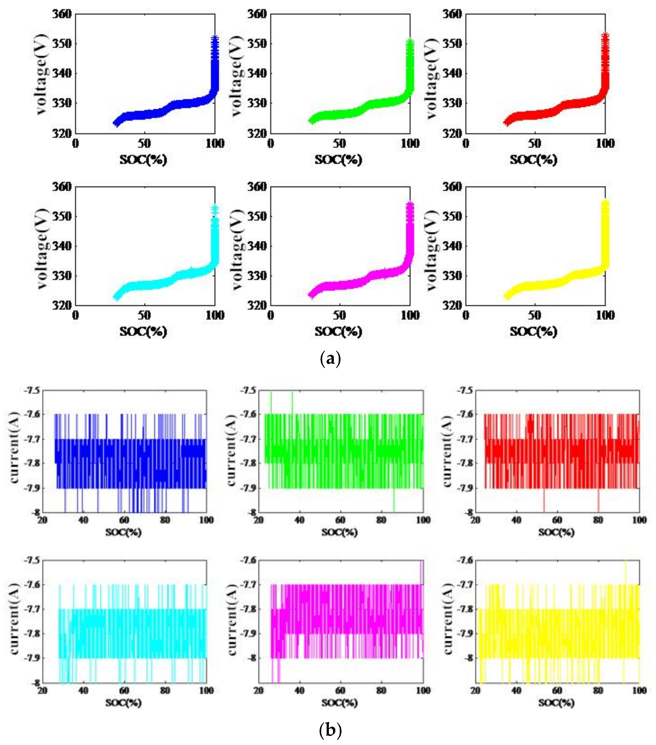
Moreover, to explore the impacts of charge voltage and current on charging processes, six sets of charging data were extracted to obtain the variation of voltage and current that increased with SOC, as shown in Figure 1.

As shown in Figure 1a, the total voltage slowly rises in most time during the charging process, and it sharply rises when the battery is about to be filled. Figure 1b presents that the total battery current is always negative and fluctuates up and down in the range of 0.4 during the charging process. Therefore, the voltage has less effect on the charging time, and charging current is relatively stable during the charging process.

4.2. Basic Regression Model

According to the data analysis results, the charged amount SOCc has a significant linear relationship with charging time. The basic regression prediction model between the charging time and charged amount SOCc is shown in Equation (3):

$$y=kx+b+\epsilon$$

(3)

where y represents the charging time of the BEV, the unit is h; x indicates the battery charged amount SOC (%) during the charging process; k and b represents the waiting parameter; and ε represents the white noise.

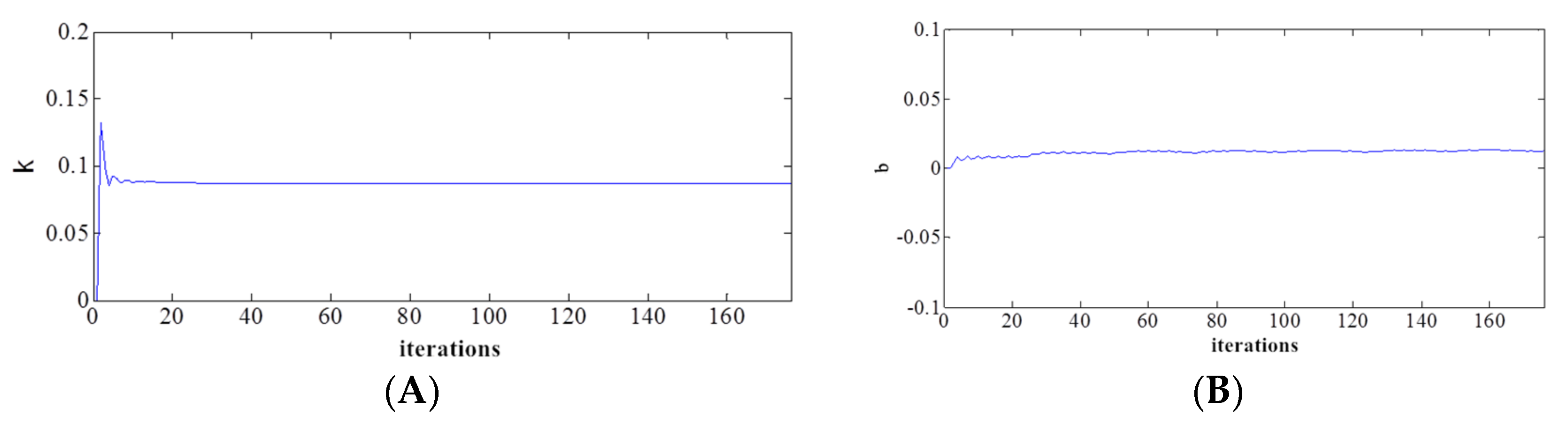
A set of representative BEV charging process data from 10:12:15 to 17:06:20 on 2 September 2016 were selected to obtain the undetermined parameters in the charging time model, as shown in Equation (3). The forgetting factor recursive least-squares algorithm [26] was adopted to realise the identification of model parameters by considering the characteristics of BEV charging data. The parameter identification results are shown in Figure 2.

The parameter identification results show that parameter k changed significantly in the initial iteration, but it soon converged and tended to be stable, and parameter b varied a little throughout the iteration. As shown in

Table 2. Parameters of charging time model.

Parameter	k	b
Value	0.0871	0.0127

, the convergence value of parameter k is 0.0871, and the convergence value of parameter b is 0.0127.

To obtain accurate parameter values, 15 arbitrary sets of BEV charging data from 1 September 2016 to 25 October 2016 were chosen to use the parameter identification method presented above for many tests and to obtain the estimated parameters, as shown in

Table 3. Parameters of charging time model.

Time (yyyy-mm-dd)	k	b
2016-09-01	0.0867	0.0118
2016-09-02	0.0871	0.0127
2016-10-03	0.0864	0.0102
2016-10-04	0.0868	0.0101
2016-09-06	0.0867	0.1324
2016-10-06	0.0783	−0.0037
2016-10-07	0.0762	0.0194
2016-10-08	0.0763	−0.0192
2016-10-09	0.0886	−0.0327
2016-10-10	0.0885	−0.0069
2016-10-15	0.0885	−0.0029
2016-10-25	0.0883	0.0001
2016-09-13	0.0877	−0.0251
2016-09-14	0.0880	0.0165
2016-09-11	0.0866	0.0133
Mean	0.0854	0.0091

.

After the parameter identification tests, the mean value of parameter k was equal to 0.0854, and the mean value of parameter b was equal to 0.0091. Therefore, the relationship model between the charging time y and the charged amount SOCc x can be expressed as:

$$y=0.0854x+0.0091+\epsilon$$

(4)

To verify the fitting effect of the model, the goodness-of-fit test and the significance test were carried out [27]. The statistical test results are shown in

Table 4. Statistical test results of regression equation.

Goodness-of-Fit Test		Linear Relationship Significance Test		Regression Coefficient Significance Test
$R^2$	$s_e$	F	$F_{0.05}$	T	$T_{0.05}$
0.951	0.043	79.88	3.925	14.40	1.98

.

As shown in Table 4, the fitting coefficient R² is 0.951 and the standard deviation $s_e$ is 0.043, indicating that the fitting effect of the model is good; F = 79.88 > $F_{0.05}$, indicating a significant linear relationship between the charged amount SOCc and the charging time; and T = 14.40 > $T_{0.05}$, indicating that the regression coefficient k = 0.0854 between the charged amount SOCc and charging time is significant.

To further verify the error of the model, the mean error (EMean), root mean square error (RMSE) and root mean square relative error (RMSRE) were used as the indexes to test the model [28] on the basis of three sets of charging data not used for modelling. The results are shown in

Table 5. Error analysis.

	EMean	RMSE	RMSRE
Data 1	0.0683	0.0815	0.0159
Data 2	0.0325	0.0420	0.0124
Data 3	0.0360	0.0432	0.0108

, where the mean error is less than 0.07, the root mean square error is less than 0.09 and the root mean square relative error is less than 0.016. In other words, the prediction error of the charging time was within 6 min. Therefore, the charging time model based on the charged amount SOCc can exactly reflect the actual charging process, which has quite accuracy and practicality.

In addition, the errors of the three groups of data were standardised to observe the distribution of the errors. The equation used to standardise the errors is:

$$z_{e_i}=\frac{y_i-{\stackrel{⌢}{y}}_i}{s_e}$$

(5)

where $z_{e_i}$ represents the standard error of the ith observed value; $y_i$ and ${\stackrel{⌢}{y}}_i$ are the predicting and actual values, respectively; and $s_e$ represents the standard deviation of the error sequence.

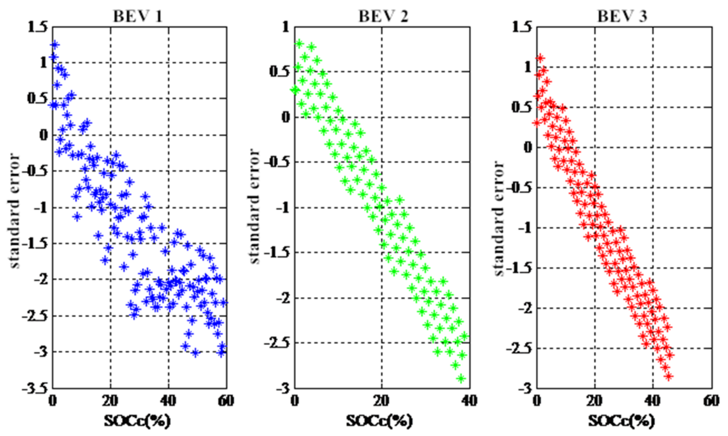
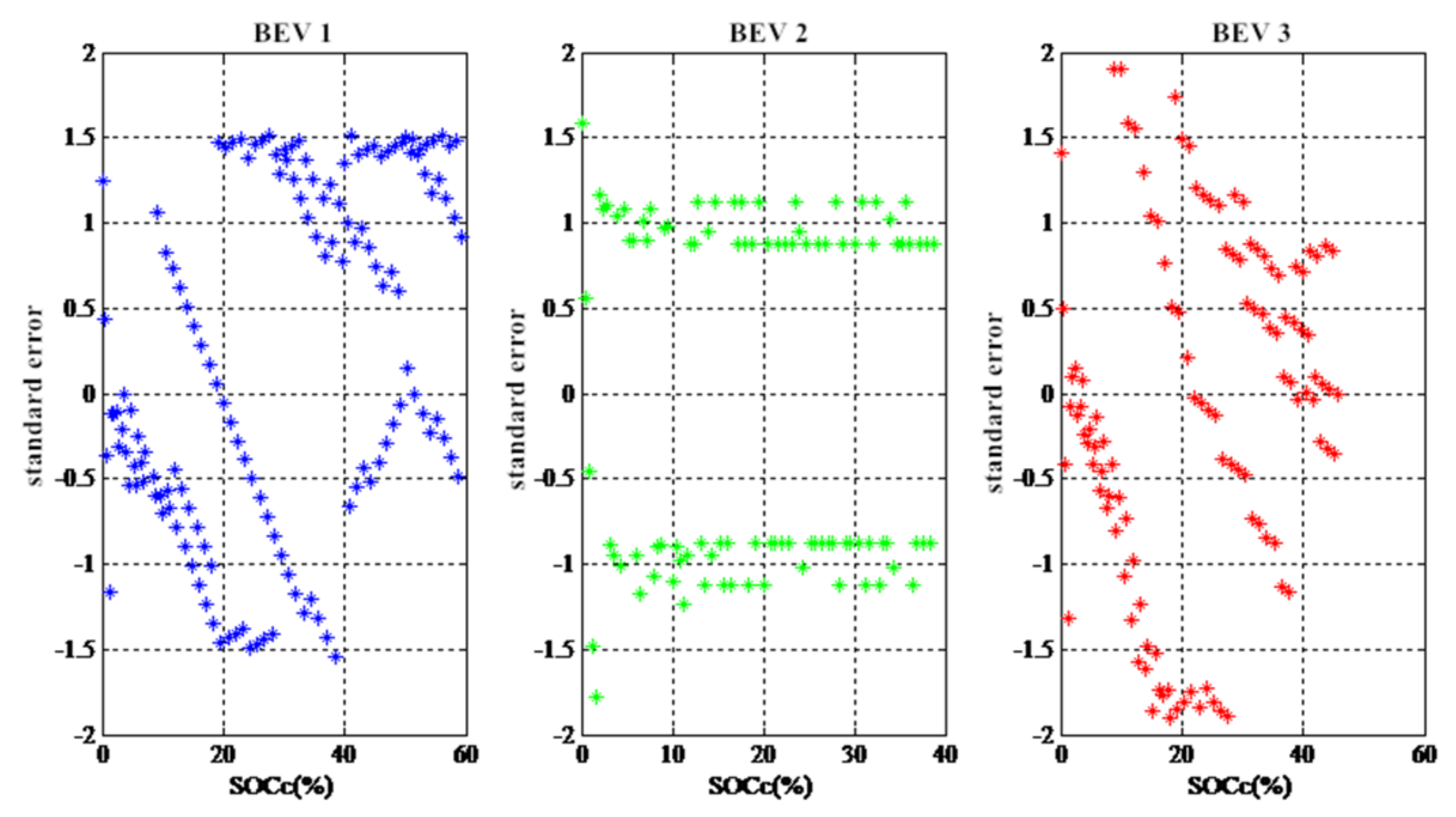
Figure 3 presents the standard error of charging time prediction. As shown in the figure, for the three BEVs, 65.5%, 79.6% and 82.6% of the standard error were found to be between −2 and 2, respectively. If the error follows the normal distribution, then approximately 95% of the normalised error between −2 and 2 should be found in the normalised error graph. The error of the charging time and the charged amount SOCc did not satisfy this condition. In other words, the error did not follow the normal distribution. Therefore, the model needs to be calibrated to obtain accurate predictions. The charged amount SOCc was regarded as a different observed point, and the corresponding error was the observed value of that point. The time-series method was applied to further modify the model.

4.3. Combined Model Based on Regression and Time-Series Methods

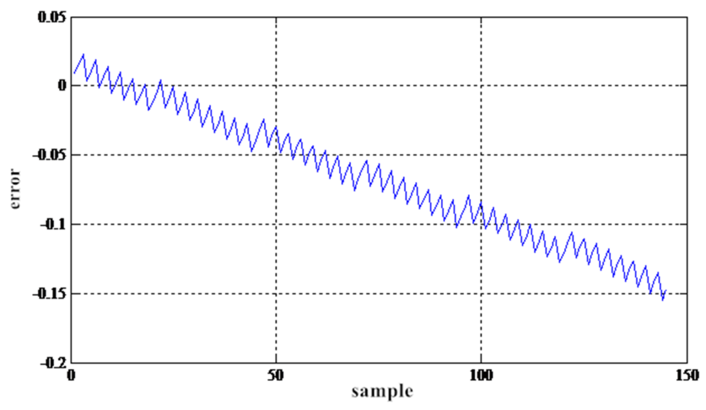
In statistics, a set of variables permutated with time sequences is called time series of random events. The modelling process of time-series method includes stability test, differential operation, white noise test and auto regression moving average (ARMA) model fitting [29]. The stability test of prediction error of data 1 in Table 5 was first operated based on the time-series modelling process. The main methods of stability test are drawing test and ADF test [30]. Figure 4 shows the sequence diagram of the estimated error of charging time. As shown in the figure, the estimated error of the charging time shows a cyclical growth trend.

Moreover, the results of autocorrelation and partial correlation indicate that the autocorrelation coefficient of the sequence decreased slowly and the autocorrelation coefficient was greater than zero in a long period of delay, which is consistent with the growth trend presented in Figure 4. Furthermore, ADF unit root test results are shown in

Table 6. ADF test results.

		t-Statistic	Prob.*
Augmented Dickey–Fuller test statistic		5.652382	1.0000
Test critical values:	1% level	−2.581349
	5% level	−1.943090
	10% level	−1.615220

; p = 1 (>0.05) as represented by Prob.* in the table. The sequence is a non-stationary sequence integrated with the chart and ADF test results.

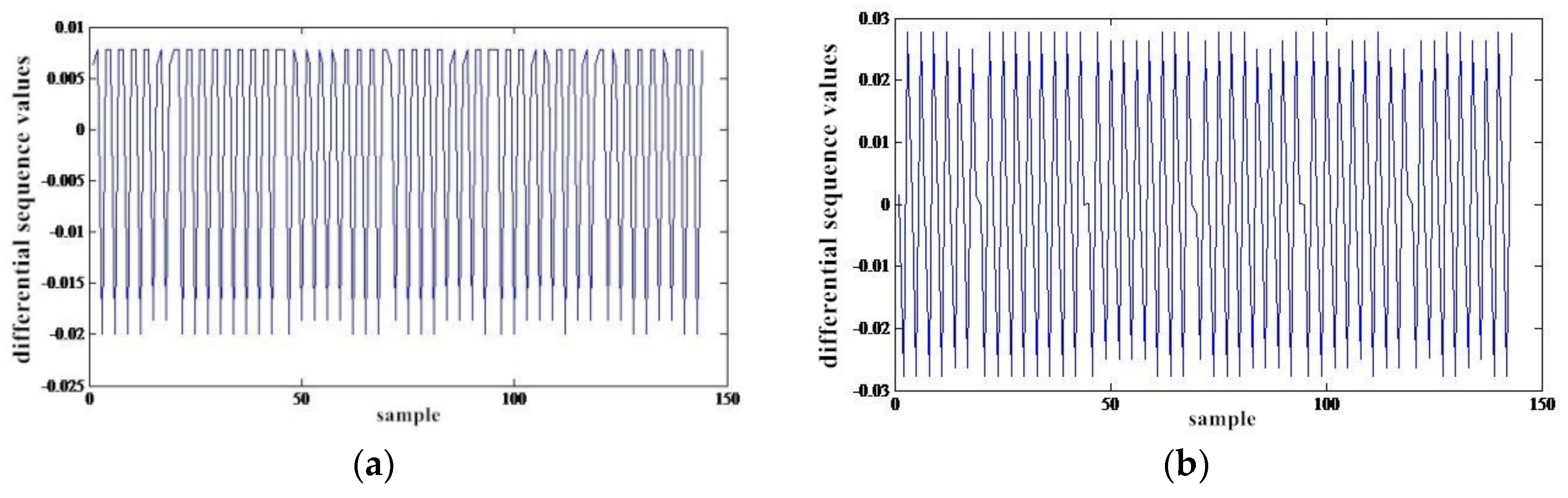
The original sequence is a non-stationary sequence, and thus the p-order difference was used to eliminate the tendency of the original sequence. First- and second-order difference results of the original sequence are presented in Figure 5.

The variances of the sequence values after first- and second-order difference were calculated. The results are shown in

Table 7. Variance after difference.

Difference	Variance
First order	0.000159
Second order	0.000469

.

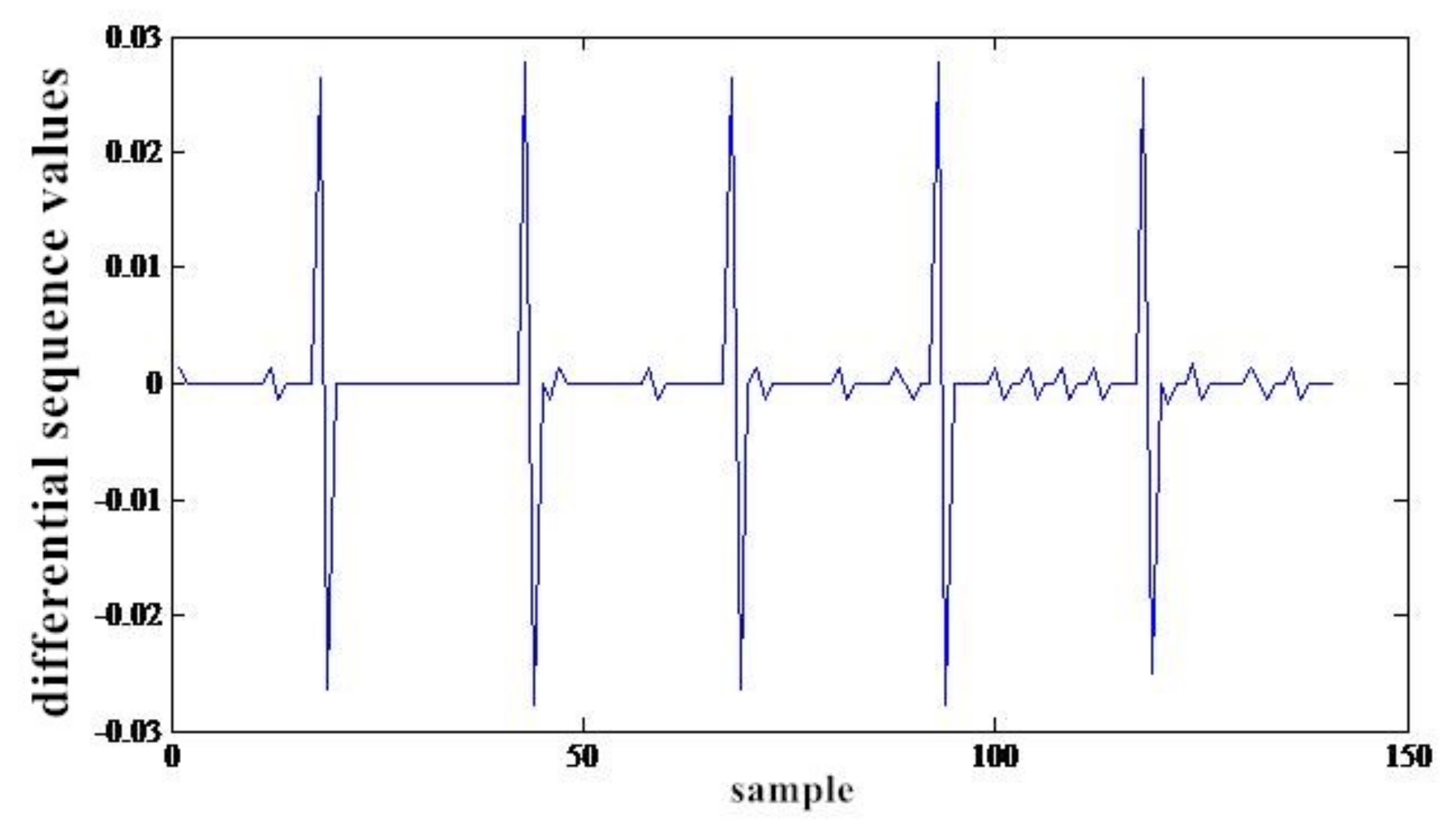
The second difference was determined as excessive difference (0.000469 > 0.000159). The first-order difference of the original sequence can eliminate its tendency. After eliminating the tendency of the original sequence, a three-step differential sequence was conducted to eliminate the cycle effect. Figure 6 presents a new sequence after the three-step differential sequence.

As shown in Figure 6, the new sequence has no significant trend or periodicity after the difference, but presents characteristics of random fluctuation. However, whether this new sequence is stationary or not is dependent on autocorrelation (partial correlation) and ADF test. ADF test results of the sequence are shown in

Table 8. ADF test result after differential sequence.

		t-Statistic	Prob.*
Augmented Dickey–Fuller test statistic		−10.02172	0.0000
Test critical values:	1% level	−2.581951
	5% level	−1.943175
	10% level	−1.615168

; p = 0 (< 0.05).

The results of autocorrelation and partial correlation of the sequence after differential sequence indicate that the autocorrelation coefficient of this sequence was rapidly reduced to 0 after a very short delay. Therefore, the sequence after difference was a stationary sequence integrated with the chart and ADF test results.

Table 9. White noise test results after differential sequence.

Order of Delay	Q	P
6	35.98	0.000
12	36.04	0.000
18	36.10	0.007

shows the results of the white noise test after difference. The value of Q is obtained by the autocorrelation coefficients of all the samples in the consideration of order of delay. The value of P is used to reflect the significant level of the autocorrelation coefficients. By observing the value of P and comparing it with the significant level of 0.05, whether the sequence is white noise can be determined. In the table, all the P values are less than the significant level of 0.05, so the sequence after the differential sequence was not white noise. Therefore, the sequence needs to be analysed.

In the model identification process, the characteristics of the autocorrelation and partial correlation graphs of the sample were used to estimate the self-correlation order [31]. As shown in Figure 6, the autocorrelation coefficient attenuation speed of sequence after difference after a delay is very fast, and the clear majority falls within a scope of two times the standard deviation. Thus, the truncation of autocorrelation coefficient can be determined; the partial correlation coefficient presents an obvious tailing phenomenon. According to the basic principles of ARMA, moving average (MA) (1) was selected initially. However, sparse coefficient model was finally selected due to the sudden increase of the autocorrelation and partial correlation coefficients in the decay process. Test results are shown in

Table 10. SSR and SE of ARMA (p, q).

Model	SSR	SE
MA (1)	0.004	0.005
MA (24)	0.004	0.005
MA (25)	0.002	0.004
MA (26)	0.004	0.005
MA (1, 24)	0.004	0.005
MA (1, 25)	0.003	0.004
MA (1, 26)	0.003	0.005
MA (24, 25)	0.002	0.004
MA (24, 26)	0.004	0.005
MA (25, 26)	0.002	0.003
MA (1, 24, 25)	0.002	0.004
MA (1, 24, 26)	0.002	0.004
MA (1, 25, 26)	0.001	0.003
MA (24, 25, 26)	0.002	0.004
MA (1, 24, 25, 26)	0.001	0.003
ARMA (24, 1)	0.003	0.005
ARMA (24, 24)	0.003	0.005
ARMA (24, 25)	0.002	0.004
ARMA (24, 26)	0.003	0.005
ARMA (24, (1, 24))	0.003	0.005
ARMA (24, (1, 25))	0.002	0.004
ARMA (24, (1, 26))	0.003	0.005
ARMA (24, (24, 25))	0.002	0.004
ARMA (24, (24, 26))	0.003	0.005
ARMA (24, (25, 26))	0.002	0.004
ARMA (24, (1, 24, 25))	0.001	0.003
ARMA (24, (1, 24, 26))	0.001	0.003
ARMA (24, (1, 25, 26))	0.001	0.003
ARMA (24, (24, 25, 26))	0.001	0.004
ARMA (24, (1, 24, 25, 26))	0.001	0.003

and

Table 11. Accuracy test of ARMA (p, q).

Model	AIC	SC	D.W
MA (1)	−7.743	−7.721	2.068
MA (24)	−7.684	−7.663	2.372
MA (25)	−8.289	−8.268	2.986
MA (26)	−7.677	−7.656	2.373
MA (1, 24)	−7.678	−7.637	2.463
MA (1, 25)	−8.020	−7.978	2.556
MA (1, 26)	−7.720	−7.679	2.065
MA (24, 25)	−8.275	−8.233	2.986
MA (24, 26)	−7.663	−7.622	2.381
MA (25, 26)	−8.275	−8.233	2.986
MA (1, 24, 25)	−8.342	−8.279	2.741
MA (1, 24, 26)	−8.298	−8.235	2.595
MA (1, 25, 26)	−8.977	−8.914	2.033
MA (24, 25, 26)	−8.261	−8.198	2.986
MA (1, 24, 25, 26)	−8.964	−8.880	2.036
ARMA (24, 1)	−7.748	−7.701	1.985
ARMA (24, 24)	−7.767	−7.720	2.133
ARMA (24, 25)	−8.337	−8.289	2.383
ARMA (24, 26)	−7.785	−7.738	2.096
ARMA (24, (1, 24))	−7.782	−7.710	2.055
ARMA (24, (1, 25))	−8.290	−8.219	2.480
ARMA (24, (1, 26))	−7.741	−7.670	1.984
ARMA (24, (24, 25))	−8.321	−8.250	2.381
ARMA (24, (24, 26))	−7.770	−7.699	2.094
ARMA (24, (25, 26))	−8.321	−8.250	2.381
ARMA (24, (1, 24, 25))	−8.570	−8.481	2.152
ARMA (24, (1, 24, 26))	−8.387	−8.292	2.011
ARMA (24, (1, 25, 26))	−8.787	−8.692	1.960
ARMA (24, (24, 25, 26))	−8.401	−8.307	2.393
ARMA (24, (1, 24, 25, 26))	−8.538	−8.420	2.093

.

According to the test results presented above, MA (1, 24, 25, 26) and MA (1, 25, 26) were selected because of their good fitting accuracy and small residual sequence. Corresponding to the structures of MA, the MA (1, 24, 25, 26) has four parameters and MA (1, 25, 26) has three parameters. The parameters of MA (1, 24, 25, 26) are denoted as $\theta (1)$, $\theta (24)$, $\theta (25)$ and $\theta (26)$. The parameters of MA (1, 25, 26) are denoted as $\theta (1)$, $\theta (25)$ and $\theta (26)$. Furthermore, the least square estimation method was adopted as the model parameter estimation method, and the parameter estimation results are shown in

Table 12. Parameter estimation results of MA (1, 24, 25, 26) and MA (1, 25, 26).

	Model	MA (1, 24, 25, 26)		MA (1, 25, 26)
Parameter
Parameter		Estimation	Standard Deviation	Estimation	Standard Deviation
$\theta (1)$		−1.006726	0.012398	−1.006598	0.011636
$\theta (24)$		−0.012397	0.028892	-	-
$\theta (25)$		0.920906	0.036437	0.907791	0.023977
$\theta (26)$		−0.892327	0.022765	−0.892138	0.022611

.

The time-series model test included parameter and model significance tests [32].

Table 13. Parameter significance test of MA (1, 24, 25, 26) and MA (1, 25, 26).

	Model	MA (1, 24, 25, 26)		MA (1, 25, 26)
Parameter
Parameter		T	P	T	P
$\theta (1)$		−81.20135	0.0000	−86.50824	0.0000
$\theta (24)$		−0.429066	0.6685	-	-
$\theta (25)$		25.27389	0.0000	37.86055	0.0000
$\theta (26)$		−39.19661	0.0000	−39.45636	0.0000

shows the results of parameter significance test.

As shown in Table 13, $\theta (24)$ is not significant; P = 0.67 (>0.05). MA (1, 24, 25, 26) did not meet the requirements; hence, MA (1, 25, 26) was selected as the final model. Based on the difference operation, the prediction combined model is as follows:

$$\{\begin{array}{l}{y}_t=0.0854x_t+0.0091+\mu (t)\\ \mu (t)={\mu }_{t-1}+{\mu }_{t-3}-{\mu }_{t-4}-1.01v_{t-1}+0.91v_{t-25}-0.89v_{t-26}+v_t\end{array}$$

(6)

where $y_t$ and $x_t$ are the charging time and charged amount SOCc in the combined model; $u(t)$ denotes the error under time-serie t; $u_{t-1}$, $u_{t-3}$, $u_{t-4}$ are the autocorrelation coefficients that are result from the reductive differential sequences; $v_t$, $v_{t-1}$, $v_{t-25}$, $v_{t-26}$ are the stochastic disturbance sequences.

A model significance test was used to verify the validity of model. A good model can fully extract the relevant information of the sequence value. In other words, the residual sequence should be a white noise sequence. Therefore, model significance test can be regarded as the residual sequence test. As shown in

Table 14. Residual sequence test of MA (1, 25, 26).

Order of Delay	LB	P
6	35.908	0.000
12	35.967	0.000
18	36.272	0.007

, MA (1, 25, 26) residual sequences $\left\{v_t\right\}$ are tested with white noise. In the table, the values of LB and P are the critical indexes for the white noise test. The value of LB is determined by the autocorrelation coefficients of all the samples under the specific order of delay. The value of P is used to reflect the significant level of the LB value. If the value of P is less than the significant level of 0.05, it indicates that the sequence is not the white noise sequence. As shown in Table 14, the P of LB are all less than the significance level of 0.05 and the residual sequence $\left\{v_t\right\}$ is not a white noise sequence. Thus, MA (1, 25, 26) did not fully extract the relevant information of the sequence value.

The prediction model of the residual sequence $\left\{v_t\right\}$ was ARMA (25, 25) through model identification, model parameter estimation and model parameter significance test. The prediction model is:

$$v_t=0.94v_{t-25}+{\epsilon }_t+0.91{\epsilon }_{t-25}$$

(7)

A white noise test was operated on the residual sequence $\left\{{\epsilon }_t\right\}$, and the results are shown in

Table 15. Residual sequence test of ARMA (25, 25).

Order of Delay	LB	P
6	1.0007	0.986
12	1.9622	0.999
18	2.8244	1.000

. As shown in the table, the P of LB was all greater than the significance level of 0.05, which determines that the residual sequence $\left\{{\epsilon }_t\right\}$ is the white noise sequence.

After the model establishment and optimisation process presented above, the final prediction combined model was:

$$\{\begin{array}{l}{y}_t=0.0854x_t+0.0091+\mu (t)\\ \mu (t)={\mu }_{t-1}+{\mu }_{t-3}-{\mu }_{t-4}-1.01v_{t-1}+0.91v_{t-25}-0.89v_{t-26}+v_t\\ v_t=0.94v_{t-25}+{\epsilon }_t+0.91{\epsilon }_{t-25}\end{array}$$

(8)

where $\left\{{\epsilon }_t\right\}$ represents the white noise sequence.

4.4. Model Validation

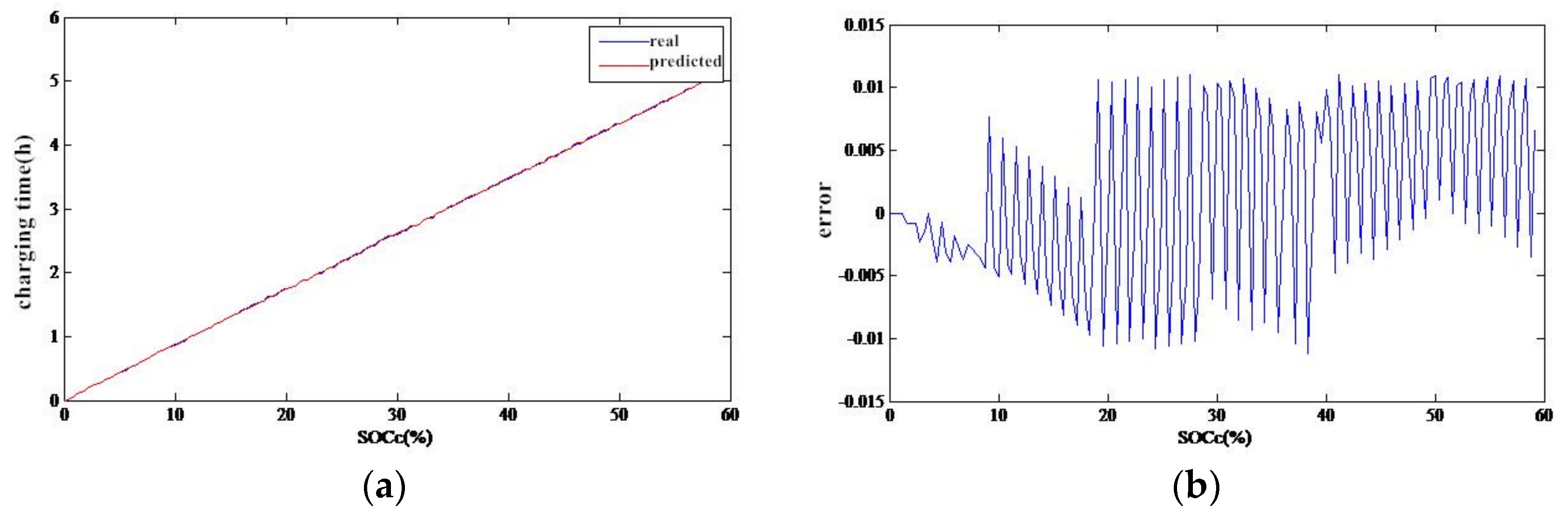
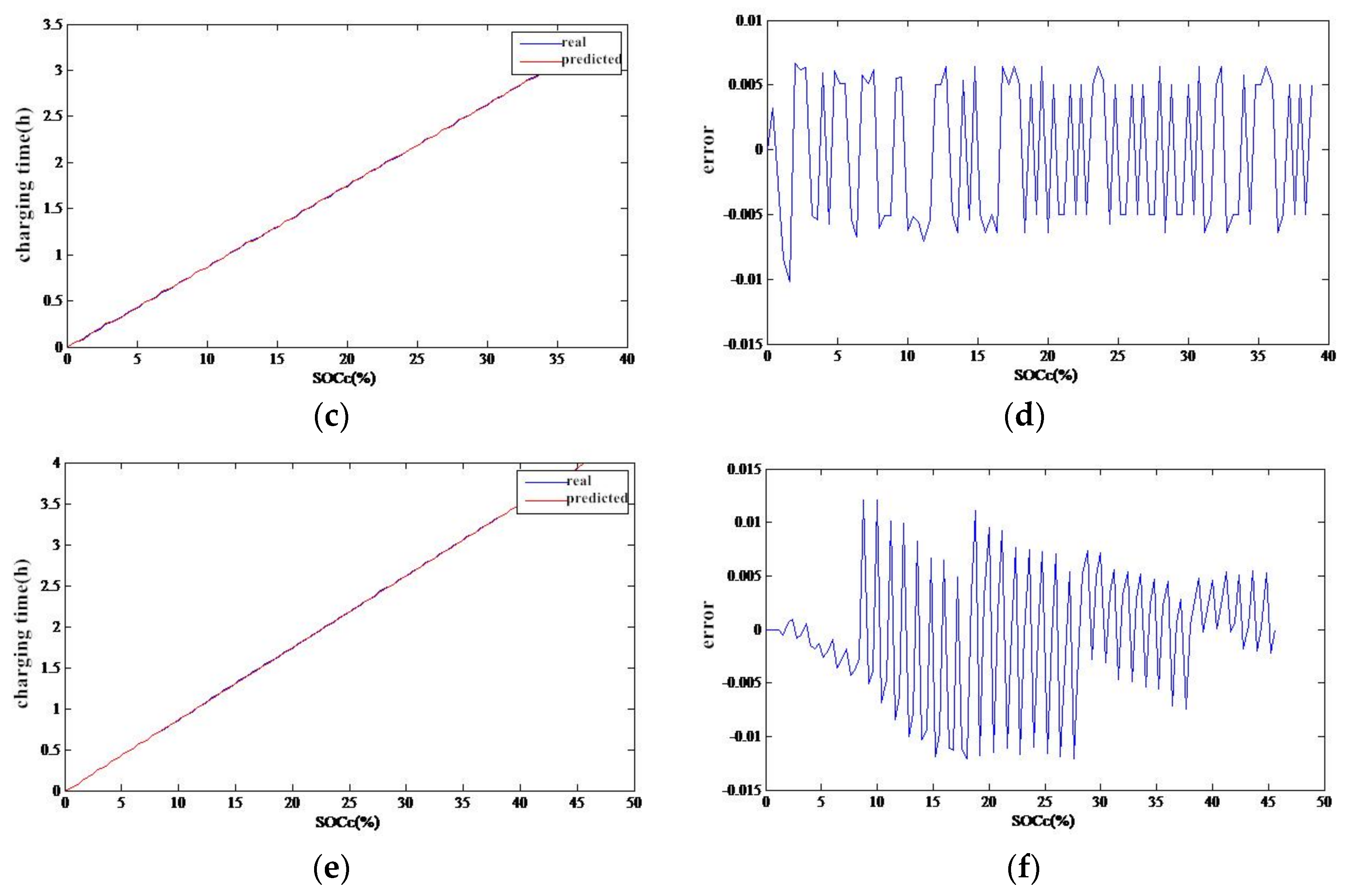
The prediction combined model of charging time, as shown in Equation (8), was obtained through the process presented above. The model was verified by the sample data shown in Table 5, and the prediction results and errors are shown in Figure 7.

As shown in the prediction results presented above, the change trend of real values is basically in line with the prediction curves. As shown in Figure 7b, errors between the predicted and real values are distributed between −0.0112 and 0.0110; as shown in Figure 7d, errors between the value and real values are distributed between −0.0101 and 0.0066; as shown in Figure 7f, errors between the predicted and real values are between −0.0145 and 0.0135. The error analysis results are shown in

Table 16. Error analysis.

	EMean	RMSE	RMSRE
Data 1	0.0063	0.0073	0.0014
Data 2	0.0053	0.0055	0.0016
Data 3	0.0052	0.0068	0.0017

.

As shown in Table 16, the mean errors are all less than 0.007, the root mean square errors are all less than 0.008 and the root mean square relative errors are all less than 0.002. In other words, the prediction error of charging time was controlled within 0.42 min. The accuracy of the charging time prediction was improved by 92% as compared with the basic regression prediction. Figure 8 shows the standard error of the charging time prediction.

As shown in Figure 8, the standard error of the three BEVs falls between −2 and 2. Evidently, the errors were normally distributed. To sum up, the combined model made the prediction of charging time accurate and practical.

5. Conclusions

The accurate prediction of charging time is an important issue for drivers of BEVs, which is very useful in determining travel plan and alleviate range anxiety during trips. In this study, actual data from 70 BEVs operating in Beijing, China, were used to explore the charging time prediction. The data completely recorded the charging processes of BEVs. After data processing, the experimental data were applied to perform the relation analysis. The results indicated a significant linear relationship between the charged amount SOCc and charging time. A basic regression model was established by using the experimental data for parameter identification based on the data analysis results. The fitting effect of the model was verified by using the goodness-of-fit and significance tests. Moreover, to further improve the accuracy of the prediction results for charging time, a time-series method was applied to calibrate the proposed model based on the actual data. Therefore, a combined model for charging time prediction based on regression and time-series methods was built. An experiment was designed to verify the combined model based on the experimental data. The standard error of the model was within a reasonable range, and the errors were normally distributed, thereby confirming that the proposed model possessed good prediction accuracy.

Notably, all experimental data were collected from BEVs operating in Beijing, which mainly records the charging processes of the vehicles. However, the external environment (such as charging station state and temperature) when charging a BEV may affect the charging time. Therefore, future research can consider the impact of external environment on charging time prediction to further improve model performance.

References

- Vidhi, R.; Shrivastava, P. A Review of Electric Vehicle Lifecycle Emissions and Policy Recommendations to Increase EV Penetration in India. Energies 2018, 11, 483. [Google Scholar] [CrossRef]
- Wang, Y.; Bi, J.; Guan, W.; Zhao, X. Optimising route choices for the travelling and charging of battery electric vehicles by considering multiple objectives. Transp. Res. Part D Transp. Environ. 2017, in press. [Google Scholar] [CrossRef]
- Rao, R.; Zhang, X.; Xie, J.; Ju, L. Optimizing electric vehicle users’ charging behavior in battery swapping mode. Appl. Energy 2015, 155, 547–559. [Google Scholar] [CrossRef]
- Ashtari, A.; Bibeau, E.; Shahidinejad, S.; Molinski, T. PEV charging profile prediction and analysis based on vehicle usage data. IEEE Trans. Smart Grid 2012, 3, 341–350. [Google Scholar] [CrossRef]
- He, H.; Xiong, R.; Chang, Y. Dynamic Modeling and Simulation on a Hybrid Power System for Electric Vehicle Applications. Energies 2010, 3, 1821–1830. [Google Scholar] [CrossRef]
- Clement-Nyns, K.; Haesen, E.; Driesen, J. The impact of charging plug-in hybrid electric vehicles on a residential distribution grid. IEEE Trans. Power Syst. 2010, 25, 371–380. [Google Scholar] [CrossRef] [Green Version]
- An, K.; Song, K.; Hur, K. Incorporating Charging/Discharging Strategy of Electric Vehicles into Security-Constrained Optimal Power Flow to Support High Renewable Penetration. Energies 2017, 10, 729. [Google Scholar] [CrossRef]
- Habib, S.; Kamran, M.; Rashid, U. Impact analysis of vehicle-to-grid technology and charging strategies of electric vehicles on distribution networks—A review. J. Power Sources 2015, 277, 205–214. [Google Scholar] [CrossRef]
- Zhang, W.; Zhang, D.; Mu, B.; Wang, L.; Bao, Y.; Jiang, J.; Morais, H. Decentralized Electric Vehicle Charging Strategies for Reduced Load Variation and Guaranteed Charge Completion in Regional Distribution Grids. Energies 2017, 10, 147. [Google Scholar] [CrossRef]
- Cui, X.; Kim, H.K.; Liu, C.; Kao, S.C.; Bhaduri, B.L. Simulating the household plug-in hybrid electric vehicle distribution and its electric distribution network impacts. Transp. Res. Part D Transp. Environ. 2012, 17, 548–554. [Google Scholar] [CrossRef]
- Kumar, K.N.; Tseng, K.J. Impact of demand response management on chargeability of electric vehicles. Energy 2016, 111, 190–196. [Google Scholar] [CrossRef]
- Aziz, M.; Oda, T.; Ito, M. Battery-assisted charging system for simultaneous charging of electric vehicles. Energy 2016, 100, 82–90. [Google Scholar] [CrossRef]
- Mukherjee, J.C.; Shukla, S.; Gupta, A. Mobility aware scheduling for imbalance reduction through charging coordination of electric vehicles in smart grid. Pervasive Mob. Comput. 2015, 21, 104–118. [Google Scholar] [CrossRef]
- Sun, X.H.; Yamamoto, T.; Morikawa, T. Fast-charging station choice behavior among battery electric vehicle users. Transp. Res. Part D Transp. Environ. 2016, 46, 26–39. [Google Scholar] [CrossRef]
- Oda, T.; Aziz, M.; Mitani, T.; Watanabe, Y.; Kashiwagi, T. Mitigation of Congestion Related to Quick Charging of Electric Vehicles Based on Waiting time and Cost-benefit Analyses: A Japanese Case Study. Sustain. Cities Soc. 2017, in press. [Google Scholar] [CrossRef]
- Awasthi, A.; Venkitusamy, K.; Sanjeevikumar, P.; Selvamuthukumaran, R.; Blaabjerg, F.; Singh, A.K. Optimal planning of electric vehicle charging station at the distribution system using hybrid optimization algorithm. Energy 2017, 133, 70–78. [Google Scholar] [CrossRef]
- Jabeen, F.; Olaru, D.; Smith, B.; Braunl, T.; Speidel, S. Electric vehicle battery charging behaviour: Findings from a driver survey. In Proceedings of the 36th Australasian Transport Research Forum (ATRF), Brisbane, Australia, 2–4 October 2013. [Google Scholar]
- Azadfar, E.; Sreeram, V.; Harries, D. The investigation of the major factors influencing plug-in electric vehicle driving patterns and charging behaviour. Renew. Sustain. Energy Rev. 2015, 42, 1065–1076. [Google Scholar] [CrossRef]
- Axsen, J.; Kurani, K.S. Who can recharge a plug-in electric vehicle at home? Transp. Res. Part D Transp. Environ. 2012, 17, 349–353. [Google Scholar] [CrossRef]
- Bunce, L.; Harris, M.; Burgess, M. Charge up then charge out? drivers’ perceptions and experiences of electric vehicles in the UK. Transp. Res. Part A Policy Pract. 2014, 59, 278–287. [Google Scholar] [CrossRef]
- Franke, T.; Krems, J.F. Understanding charging behaviour of electric vehicle users. Transp. Res. Part F Traffic Psychol. Behav. 2013, 21, 75–89. [Google Scholar] [CrossRef]
- Adornato, B.; Patil, R.; Filipi, Z.; Baraket, Z.; Gordon, T. Characterizing naturalistic driving patterns for Plug-in Hybrid Electric Vehicle analysis. In Proceedings of the IEEE Vehicle Power and Propulsion Conference (VPPC’09), Dearborn, MI, USA, 7–10 September 2009; pp. 655–660. [Google Scholar]
- Zhong, F.; Li, H.; Zhong, S.; Zhong, Q.; Yin, C. An SOC estimation approach based on adaptive sliding mode observer and fractional order equivalent circuit model for lithium-ion batteries. Commun. Nonlinear Sci. Numer. Simul. 2015, 24, 127–144. [Google Scholar] [CrossRef]
- Calvi, J.P.; Manh, P. Lagrange interpolation at real projections of Leja sequences for the unit disk. Proc. Am. Math. Soc. 2012, 140, 4271–4284. [Google Scholar] [CrossRef]
- Kenett, D.Y.; Tumminello, M.; Madi, A.; Gurgershgoren, G.; Mantegna, R.N.; Benjacob, E. Dominating clasp of the financial sector revealed by partial correlation analysis of the stock market. PLoS ONE 2010, 5, e15032. [Google Scholar] [CrossRef] [PubMed] [Green Version]
- Deng, Z.; Cao, H.; Li, X.; Jiang, J.; Yang, J.; Qin, Y. Generalized predictive control For fractional order dynamic model of solid oxide fuel cell output power. J. Power Sources 2010, 195, 8097–8103. [Google Scholar] [CrossRef]
- Fan, J.; Huang, L.S. Goodness-of-fit tests for parametric regression models. J. Am. Stat. Assoc. 2001, 96, 640–652. [Google Scholar] [CrossRef]
- Feng, S.; Wu, C.D.; Zhang, Y.Z.; Jia, Z.X. Grid-based improved maximum likelihood estimation for dynamic localization of mobile robots. Int. J. Distrib. Sens. Netw. 2016, 2014, 1–15. [Google Scholar] [CrossRef]
- Längkvist, M.; Karlsson, L.; Loutfi, A. A review of unsupervised feature learning and deep learning for time-series modeling. Pattern Recognit. Lett. 2014, 42, 11–24. [Google Scholar] [CrossRef]
- Yang, T.Y.; Yang, Y.T.; Josifidis, K. A study on the asymmetry of the news aspect of the stock market: Evidence from three institutional investors in the Taiwan stock market. Panoeconomicus 2015, 62, 361–383. [Google Scholar] [CrossRef]
- Hasan, M.K.; Hossain, N.M.; Naylor, P.A. Autocorrelation model-based identification method for ARMA systems in noise. IEE Proc. Vis. Image Signal Process. 2005, 152, 520–526. [Google Scholar] [CrossRef]
- Chen, P.; Pedersen, T.; Bak-Jensen, B.; Chen, Z. ARIMA-based time series model of stochastic wind power generation. IEEE Trans. Power Syst. 2010, 25, 667–676. [Google Scholar] [CrossRef]
Figure 1.
Charge voltage and current of six charging processes. (a) Charge voltage and SOC; (b) Charge current and SOC.
Figure 2.
Identification result of parameters for basic regression prediction model. (A) Identification result of parameter k; (B) Identification result of parameter b.
Figure 3.
Standard error of charging time prediction.
Figure 4.
Charging time estimate error sequence.
Figure 5.
First- and second-order difference results of the original sequence. (a) First-order differential sequence; (b) Second-order differential sequence.
Figure 6.
Three-step differential sequence.
Figure 7.
Prediction results and errors of the prediction combined model of charging time. (a) Prediction of charging time of data 1; (b) charging time prediction error of data 1; (c) prediction of charging time of data 2; (d) charging time prediction error of data 2; (e) Prediction of charging time of data 3; (f) charging time prediction error of data 3.
Figure 8.