A Novel Approach for Searching the Upper/Lower Bounds of Uncertainty Parameters in Microgrids


1
State Key Laboratory of Advanced Electromagnetic Engineering and Technology, School of Electrical and Electronics Engineering, Huazhong University of Science and Technology, Wuhan 430074, China
2
School of Automation, Ministry of Education Key Laboratory of Image Processing and Intelligence Control, Huazhong University of Science and Technology, Wuhan 430074, China
3
School of Electronic Information and Communications, Huazhong University of Science and Technology, Wuhan 430074, China
*
Author to whom correspondence should be addressed.
Energies 2018, 11(5), 1035; https://doi.org/10.3390/en11051035
Submission received: 31 March 2018
/
Revised: 19 April 2018
/
Accepted: 20 April 2018
/
Published: 24 April 2018
Abstract
:In this study, a novel method based on analysis is presented to search for the upper/lower bounds of uncertainty parameters in microgrids (MGs). It is well known that uncertainty parameters have important effects in a MG, and they may cause instability. Previous studies have mainly focused on identifying the stability of a MG with its uncertainty parameters, but they did not address the problem of the upper/lower bounds of uncertainty parameters, i.e., how far the uncertainty parameters can be extended while the system remains stable in the small-signal sense. Thus, we developed an approach for identifying the bounds of uncertainty in MGs. In the current paper, first, a method is proposed for linear fractional transformation (LFT) configuration to express the uncertainty parameters, which makes the stability of the nominal MG system independent of any extension of the bounds. An algorithm based on this configuration is then designed to find the upper/lower bounds for both single parameter and multiple uncertainty parameters in a MG. Finally, the two cases are discussed, and the accuracy of the proposed method is confirmed using the conventional eigenvalue method.
1. Introduction
Microgrids (MGs) have attracted much attention throughout the world because of their significant benefits for utility networks in terms of loss reduction and reliability improvement [1]. Most of the generators in an MG are distributed generation (DG) units, which interface with the utility grid through an ac/dc inverter [2]. However, the inverter does not have the same moment of inertia as a synchronous generator, so the problem of MG stability has attracted considerable attention [3,4,5,6,7,8,9,10,11,12,13,14,15]. Previous studies regarding this issue have focused mainly on the stability of (1) systems with fixed parameters; and (2) systems with uncertainty parameters. In the former systems, the values vary in a range around the nominal value [4], and they are used to represent perturbations in the equipment parameters, load changes, and controller parameters [4,5,6,7]. The major approaches used to investigate the stability of systems with fixed parameters are the eigenvalue method [8,9,10,11] and the impedance-based method [12,13,14,15,16]. In systems with uncertainty parameters, the parameters can be regarded as parameters that vary within a certain range, but the aforementioned approaches are not suitable in this case because the computational burden increases considerably for a sequence of parametric changes. In particular, multiple uncertainty parameters are present in the system, and thus, analysis must be be employed [5,6,7,17,18,19].
Previous studies have focused on the stability of systems. However, it is also very important to establish the stability margin for a system in terms of its parameters and to calculate its range of stability. The main techniques employed to address this problem for fixed parameters are the eigenvalue method [20,21] and the bifurcation method [22,23,24,25,26]. The eigenvalue method needs to determine the dominant eigenvalue as a function of the parameters. In order to reduce the computational burden associated with the eigenvalue method, modified approaches have been proposed, such as the eigenvalue sensitive algorithm [27,28] and the continuation of invariant subspaces method [29]. Other techniques for addressing this problem are bifurcation methods, such as the Hopf bifurcation [22,23], saddle-node bifurcation [24,25], and structure-induced bifurcation [26]. An advantage of these methods is that they can directly calculate the variable values of parameters that make the eigenvalue cross the stability boundary.
To the best of our knowledge, no previous studies have addressed this issue with respect to uncertainty parameters. In fact, uncertainty parameters have important effects on the stability of MGs, and they are considered fully in stability estimates [16,17,18,19,30,31,32,33]. Therefore, it is necessary to establish the stability margin of a system in terms its the uncertainty parameters and to obtain its upper/lower bounds. It should be noted that although the super upper value of the largest structured singular value (SSV) of a system is an accurate index for determining the stability of a system in the presence of uncertainty parameters, this value cannot be treated as the stability margin with respect to the uncertainty parameters. This is because the inverse of the super upper value of the largest SSV only indicates the allowable margin of deviation from the nominal value. The system is determined as unstable regardless of whether the lower bound of the parameter decreases or the upper bound of the parameter increases. Moreover, if multiple uncertainty parameters are considered, the relationship between the inverse of the super upper values of the largest SSV and the stability boundaries of the parameters will be much more complex.
In the present study, we developed an approach to search for the bound of an uncertainty parameter in an MG. In the current paper, first, a linear fractional transformation (LFT) method is introduced to express an uncertainty parameter. The frameworks for the DG unit and MG are then constructed. We also propose an algorithm for identifying the upper/lower bounds of an uncertainty parameter. The proposed method is used to study the parameters for a droop controller in an MG. The selection of these parameters is based on the following consideration: the parameters for a droop controller are determined during the operation of the system, but the parameters have no defined values and they are only are subject to a few constraints [4], and thus, different designers may select different values. Therefore, the droop parameter can be treated as an interval variable, and it is necessary to evaluate the system’s margins in terms of different parameters. Finally, in order to provide a comprehensive evaluation of the proposed method, two case studies are performed. In the first case study, we search for the upper/lower bounds of a single uncertainty parameter. In the second case study, we demonstrate the capacity of the proposed approach to identify the stability boundaries for multiple uncertainty parameters. The stability boundaries obtained are confirmed using the eigenvalue method.
The main contributions of this study are summarized as follows:
- (1)
- An algorithm is proposed to search for the upper/lower bounds of uncertainty parameters in MGs. In addition, a method is proposed for LFT to configure the uncertainty parameters, which has general applicability to the determination of uncertainty parameters.
- (2)
- The method for configuring DG units is described in detail, and it can readily be extended to an MG with multiple sources. Based on theoretical procedures, we demonstrate how to study the uncertainty parameters in other MG structures.
- (3)
- If this method is applied correctly, it is possible to accurately identify the stability boundaries for uncertainty parameters.
2. Problem Statement
2.1. Description of an MG and Its Controller
Figure 1 shows a schematic illustrating an MG and its control structure. The MG comprises two electronically-coupled DG units and a three-wire balanced load. In each DG unit, the inverter is supplied by a DC voltage source, and it is integrated into the MG through an LCL lower pass filter and inductive wire. During normal operation, the MG is connected to the utility through an intelligent bypass switch (IBS), and it supplies power together with the grid. When the grid is absent, the IBS is open and the MG enters the islanded mode, which supports the frequency and voltage of the system. The control strategy for the DG unit in island mode is based on three loops [31], i.e., an outer loop control shares the load by employing the droop strategy, a middle loop follows the reference voltage using a proportional-integral regulator, and an inner loop enhances the system’s dynamic response capacity via a proportion controller.
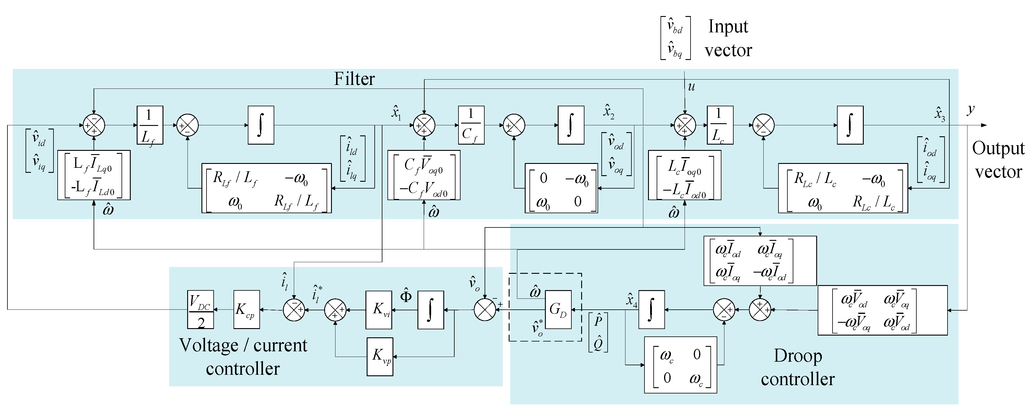
As shown in Figure 2, an analogue block diagram of a DG unit and the control loop are built in the rotating reference frame. In the block diagram, the currents of two inductors, and , the voltage of the capacitor, , the outputs average power, and , and the virtual variable, are taken as the state variables. The external input and output variables are and , respectively. Details of the mathematical derivations and the sign convention are explained in Appendix A.
2.2. The Impact of Droop Parameters on Microgrid Stability
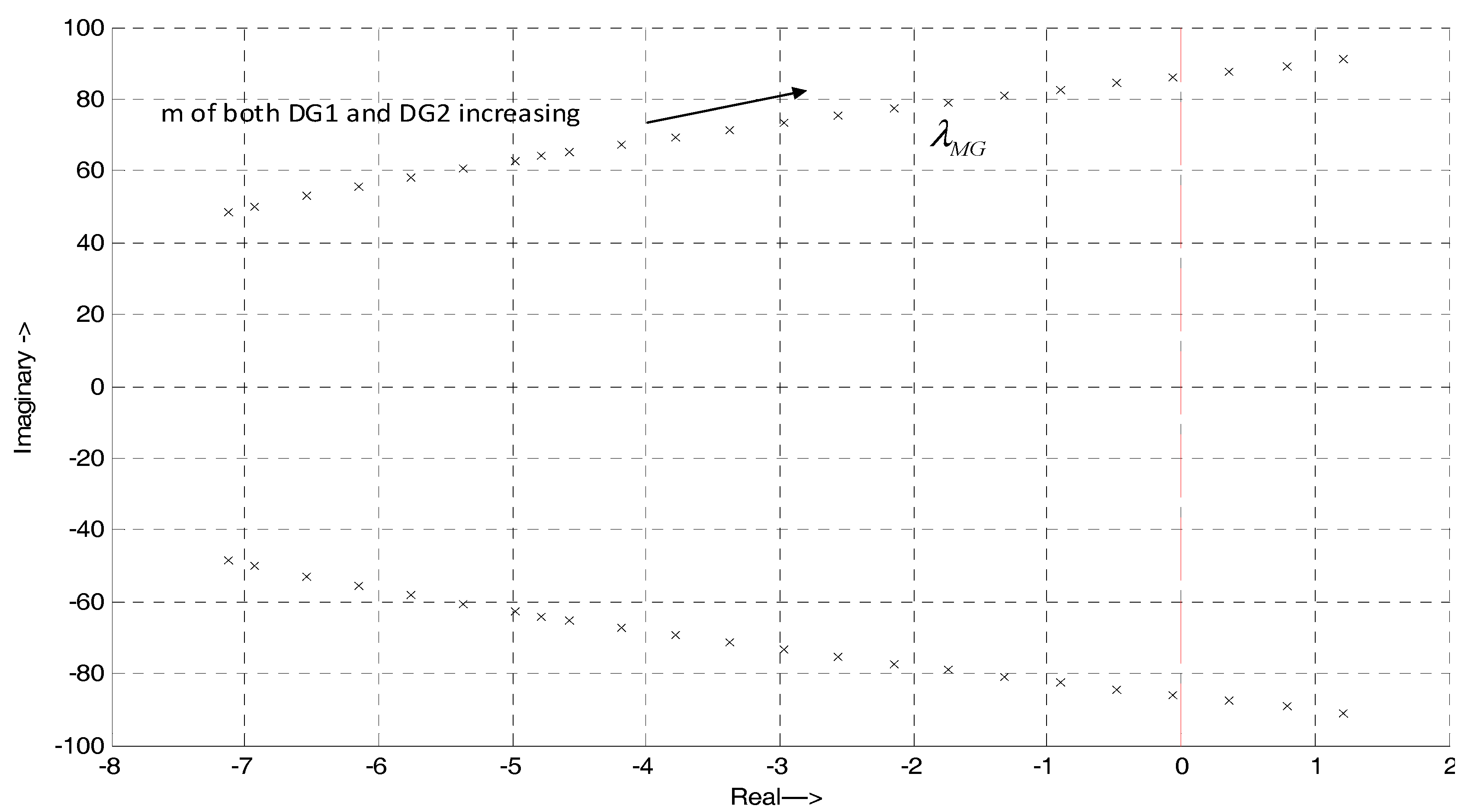
To consider the impact of the droop parameters on the stability of the MG, an eigenvalue analysis of the MG was conducted based on the small-signal model in Figure 1. Figure 3 shows the locus plots of the dominant eigenvalues as functions of the frequency droop parameter. Clearly, as the frequency droop parameter increases, the eigenvalues move toward the unstable region, which indicates that the stability margin of the MG is reduced. If the eigenvalues are sufficiently close to the positive axis, then even small fluctuations in the droop parameters can have considerable effects on the system’s stability. Large droop parameters can make the MG more oscillatory and lead to instability, but they may effectively improve the transient response of the DG unit [2]. In general, designers balance the tradeoff between the transient response and the stability when setting droop parameters. Therefore, considering that droop parameters play important roles in a system’s stability, and because of the system’s actual characteristics, it is necessary to study the stability boundaries for the droop parameters.
3. Methodology
3.1. Analysis of the Stability of a System with Uncertainty Parameters
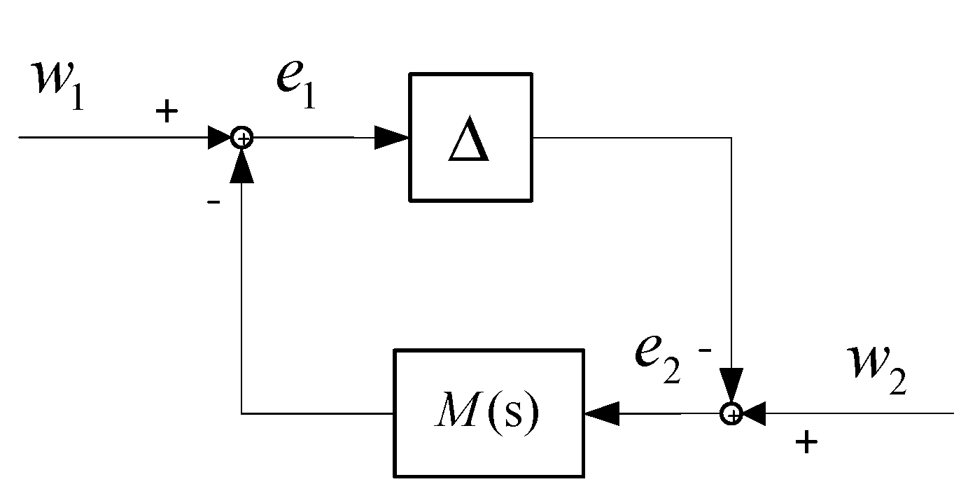
analysis [32] is a method used for examining whether a structured perturbation system is stable. Figure 4 shows the standard configuration of a structured perturbation system, where denotes the transfer function of a nominal system, and represents the “parametric uncertainty” of the system, and both are stable and bounded. It is assumed that the block structure, , has been normalized, i.e., . According to the definition of the analysis, if and only if the inequality relationship, , is satisfied, then the structured perturbation system is stable with respect to , where represents the super upper value of the largest SSV of in the frequency domain. In contrast, if , then the structured perturbation system is unstable with respect to . Therefore, the super upper value of the largest SSV can be treated as an index for identifying the stability of a perturbation system.
It should be noted that two limitations of the analysis need to be addressed: the system needs to be represented as the configuration before the analysis, and a stable is the premise for the analysis. These limitations constrain the configuration of , and they are fully considered in the proposed algorithm. In order to satisfy these limitations, we introduced a method to build the LFT configuration for the uncertainty parameters.
3.2. Proposed Method for Configuring an MG
3.2.1. Proposed LFT Configuration for Uncertainty Parameters
Figure 2 shows a block diagram of a DG unit. In general, an MG employs the droop strategy to share the load in the islanded mode. Let and be the terminal active power and reactive power of a DG unit, respectively, and and are the output reference voltage and frequency of the droop controller. The transfer function of droop controller, , from input to output is expressed as [31]:
where .
As explained previously, the parameters and are treated as interval variables in this study. In general, a parameter, , that is bounded in the region can be represented as a perturbation of its nominal value, [32]:
where and .
In Equation (2), the perturbation of a parameter is described in two parts, where denotes the mathematical perturbation and is the named size coefficient representing the size of the perturbation. Thus, the frequency droop parameter, , and the voltage droop parameter, , can be expressed as Equations (3) and (4), respectively:
where and are the nominal values of parameters and , respectively, and and are the named size coefficients which adjust the size of the interval for each parameter.
After substituting Equations (3) and (4) into Equation (1), the transfer function, , is as follows:
By employing the LFT method, the perturbations in the transfer function, , are extracted and arranged in a diagonal matrix, . Correspondingly, the transfer function, , is expanded and the fictitious vectors are introduced as the increased input and output vectors. The configuration for is depicted in Figure 5.
In Figure 5, the fictitious vectors, and , represent the input vector and the output of the perturbation block, , respectively. The transformations are given by
where
such that
It should be noted that the matrix can be decomposed in different ways, and the matrices , , and have other solutions. In this study, all of the size coefficients were arranged in block where the output was the fictitious vector, . This arrangement ensured that the stability of the nominal system was independent of the coefficients, and , as explained in Section 3.3.
3.2.2. Framework of the MG for Analysis
The models of the controllers and the circuits for the DG unit are shown in Figure 2. By substituting the LFT configuration, , into uncertainty model in the analogue block diagram, the state-space small-signal expressions of DG with uncertainty parameters can be obtained:
where are the state vectors of the DG unit. The input vectors are and , and the output vectors are and . is the angular frequency of the common reference frame, and represents the angle between the individual reference frame and the common reference frame. The matrices for , , , , , and are as follows:
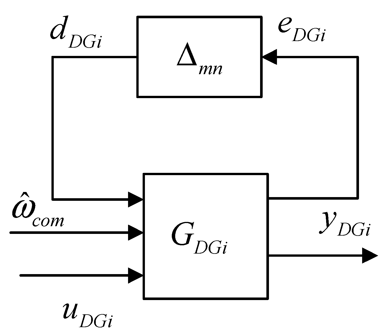
It should be noted that although this model is similar to the small-signal models presented Mohamed and El-Saadany [3], the difference between the two models is obvious because the uncertainty is integrated into the droop parameters of the DG unit in the present study, which changes the configuration of the DG unit. The configuration for the DG unit with the uncertainty parameter is shown in Figure 6, where , represented by Equations (7)–(9), denotes the transfer function matrix of the nominal model of the DG unit. The perturbation block, , represents the variations in the droop parameters.
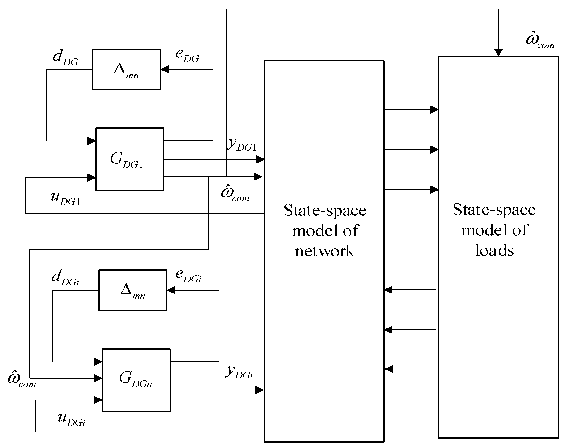
To obtain the small-signal model for the MG, the DG unit described by Equations (7)–(10) is combined with those for the load and network. This combination is shown in Figure 7, and the mathematical derivations are presented in Appendix B. The complete state-space expressions for the MG are as follows:
In Equations (11)–(13), the system state matrices, , , and , are as follows:
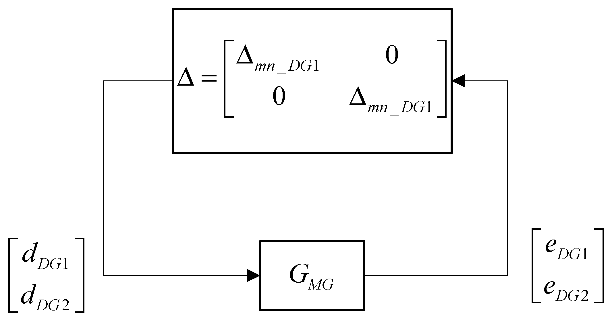
where , , , , , , , , , , , and are given in the Appendix B. The configuration for Equations (11)–(13) is shown in Figure 8.
It should be noted that coefficients and are excluded from matrix due to the proposed arrangement for the uncertainty parameter. In fact, after LFT divides the perturbation function, , into the nominal function, , and uncertainty blocks, , the fictitious output vector, , of the nominal function does not participate in the calculation of the state equations of the DG system Furthermore, Figure 7 shows that the fictitious vector, , which comprises all of the fictitious vectors, , in each DG unit still does not participate in the calculation of the state equations for the nominal system, . Therefore, the stability of the nominal system, , is independent of coefficients and under this configuration. The proposed configuration accurately represents the system with parameter variations, and it is suitable for the subsequent analysis.
3.3. Stable Upper/Lower Bound Analysis for a Single Uncertainty Parameter
After the MG with uncertainty parameters has been described using Equations (11)–(13), the value can reflect the stability of the MG with respect to a given parameter within a certain range. For convenience, we consider parameter instead of parameter or in the following explanation. First, we discuss the case with only one uncertainty parameter in an MG. According to the definitions, if the value of is less than 1, the MG is stable and parameter takes any value within the range of . In contrast, when is greater than 1, this indicates that this range is greater than the stability boundary for parameter . Based on this fact, we propose the following method for identifying the upper/lower bounds of an uncertainty parameter.
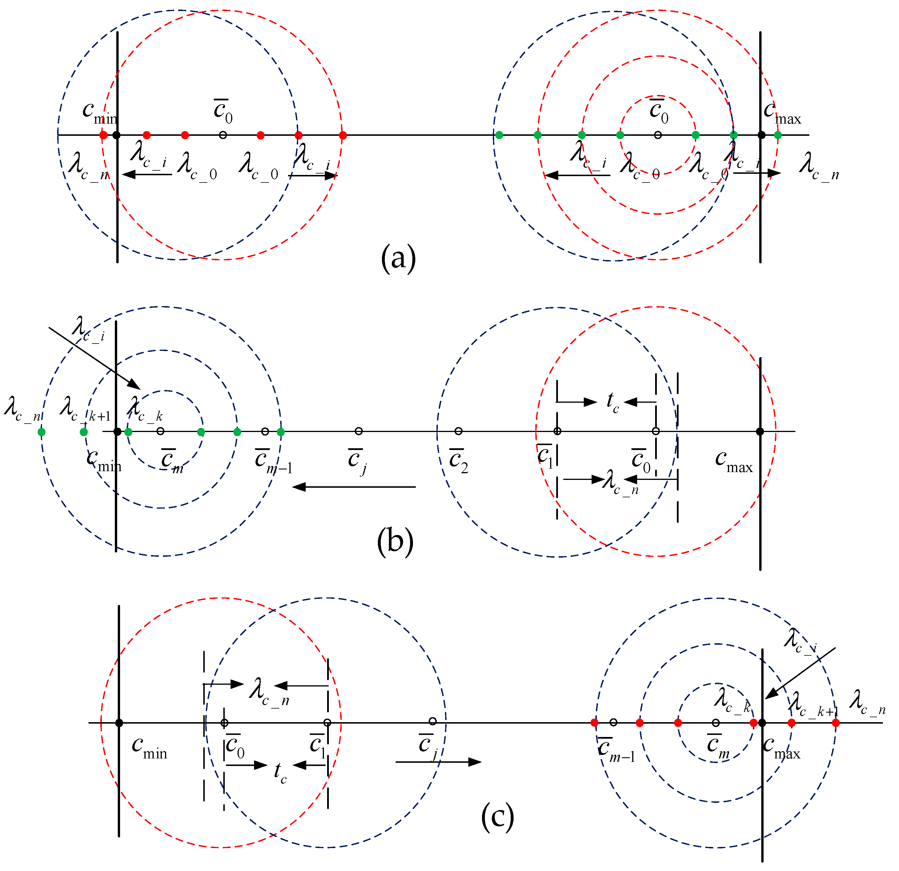
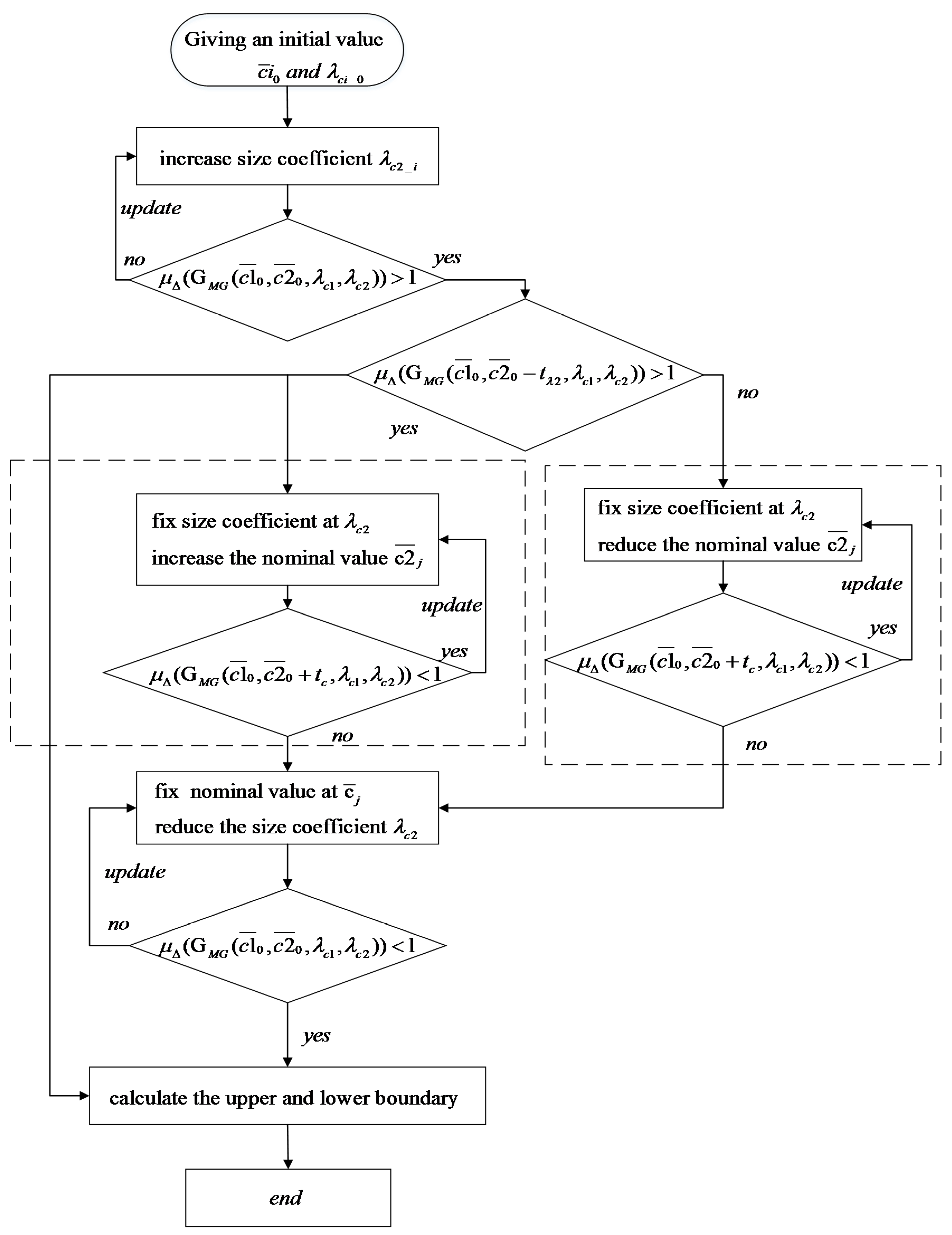
First, the value is initiated as the operating value for the MG and the size coefficient, , is set. The size coefficient, , is then increased in steps of to extend the interval of parameter . The iterative process is completed up to a value of , which makes greater than 1. As shown in Figure 9a, two possible options can trigger to exceed 1: the extension of the interval to reach the lower bound of parameter if the initial value, , is near the lower bound; or if the value of is close to the upper bound, the upper bound of parameter is reached first.
To determine the most appropriate possible option, the size coefficient is fixed at , and the nominal value, , is reduced by a step, . If the value of changes to less than 1, the trigger is the upper bound of the parameter, and it must fall within the interval of ; otherwise, if the value of remains greater than 1, the trigger is the lower bound, where the value is limited within . Theoretically, the size coefficient that makes closest to 1 denotes the maximum size of the perturbation of parameter . However, it is difficult to satisfy this condition because it incurs considerable computational burden. Thus, it is replaced by the maximum size coefficient to make no more than 1. For instance, is selected as the maximum size of the perturbation, and the upper bound of is taken as . This selection will make the error no more than step value .
For the other bound of uncertainty parameter , we first consider the case where the previous trigger is the upper bound of parameter . To identify the lower bound of , the size coefficient is fixed at according to the steps shown in Figure 9a, and the nominal value, , is reduced in steps of . As shown in Figure 9b, as decreases, the interval slides to the left so the system enters a stable state again. Up to the point where the lower bound of the uncertainty parameter is included in the interval, the value of will change to exceed 1; the lower bound of the parameter is subsequently within the interval of . To further identify the accurate point for the lower bound, is then fixed and decreases in steps of to narrow the interval. According to the theoretical analysis, if the lower bound is outside the range of , then the value of becomes smaller than 1. Hence, the lower bound of the parameter can be taken as . Similarly, if the previous trigger is the lower bound of the parameter, the upper bound of parameter can also be obtained in this manner. This process is shown in Figure 9c.
The key to this method is satisfying the requirement of the analysis that the nominal system, , should be stable. This requirement can be classified with two cases, as follows. In the first case, we consider how changing the size coefficient, , affects the stability of when the nominal parameter, , is fixed. Clearly, the stability of nominal system is determined by matrix of system state space expressions. However, in the proposed method, coefficients and are not introduced into matrix , and thus the internal stability of the nominal system, , remains the same as the steady state regardless of how the size coefficients change.
In the second case, we consider that the size coefficient is fixed at , and we need to ensure the stability of nominal system when the nominal parameter varies from to . According to the analysis, if the size coefficients have no impact on the stability of the nominal system, then the conditions in which the perturbation system is stable with respect to in the range of can ensure that the nominal system is stable with respect to parameter in the same range. Thus, this condition is satisfied provided that step does not exceed step . In the proposed method, the value of is set as equal to .
3.4. Analysis of Stability Boundaries for Two Uncertainty Parameters
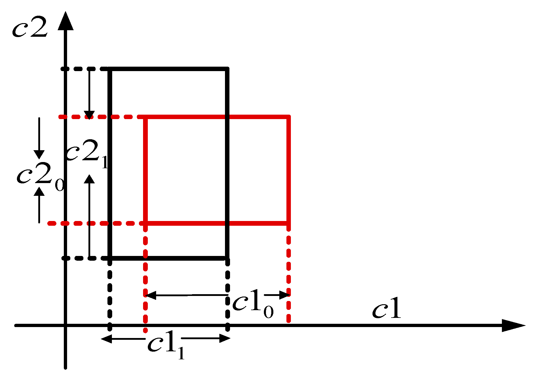
In this problem, we note that for an uncertainty parameter, , there is a stability boundary, , for the uncertainty parameter under the MG, as shown in Figure 10. The stability boundaries of the two uncertainty parameters comprise many of these areas. Therefore, obtaining the stability boundary, , for a given uncertain parameter, , is crucial for solving this problem. Therefore, we assume that parameter can be expressed as
where represents the mean of in the range and .
By substituting and from Equation (14) into Equations (11)–(13), the problem of searching for stable boundaries for and can be simplified as identifying the stability boundary of a single parameter, . The details of the algorithm are given in Figure 11, and the search process is depicted in Figure 12, where the vertical axis denotes the predetermined range of , and the horizontal axis represents the range of .
4. Study Cases
Next, we present examples to demonstrate how the proposed method can be used to obtain the upper/lower bounds of uncertainty parameters in the MG shown in Figure 1. The nominal values of the system parameters are given in Table 1. Two cases were considered in this study: (1) searching for the stability boundary for a single uncertainty parameter; and (2) searching for two uncertainty parameters in the MG. The eigenvalues of the uncertain MG under the parameters in the boundary obtained were calculated to verify the result.
4.1. Case 1: Analysis of the Upper/Lower Stability Bounds for a Single Uncertainty Parameter
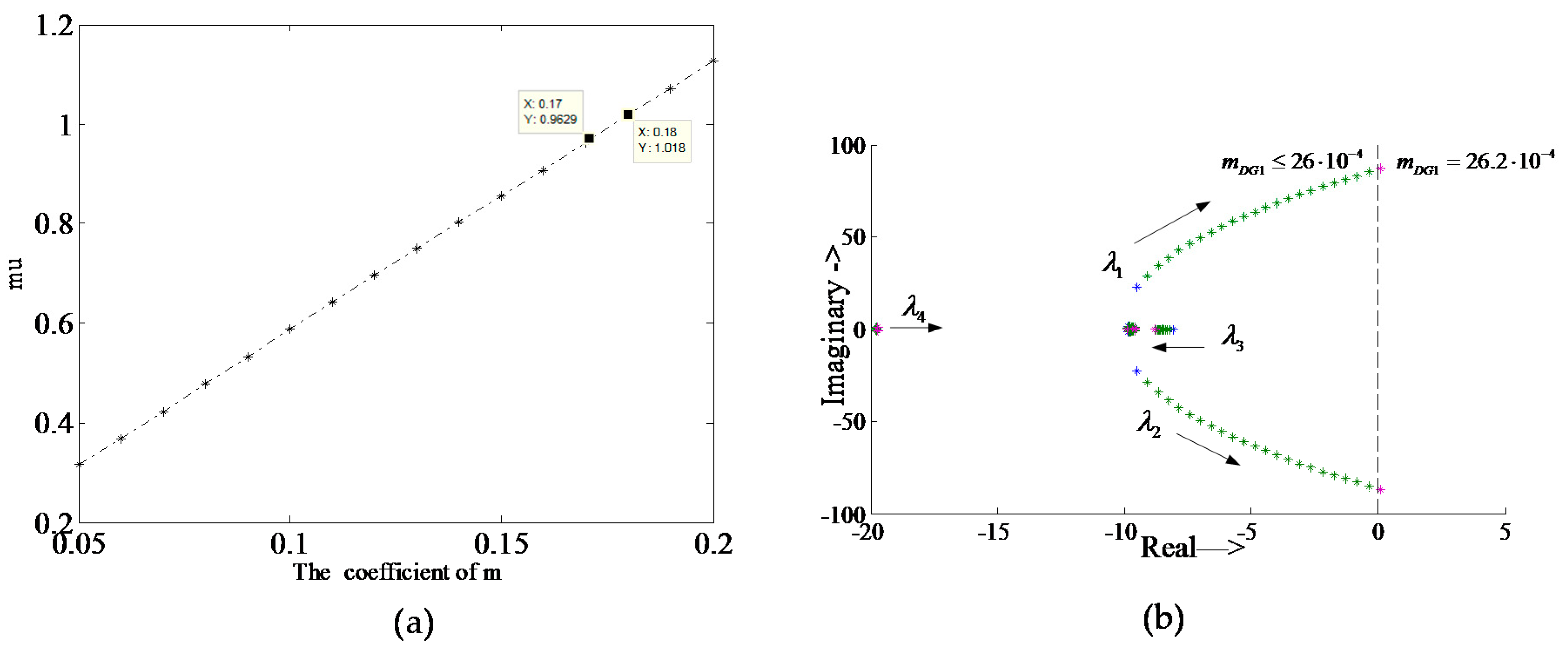
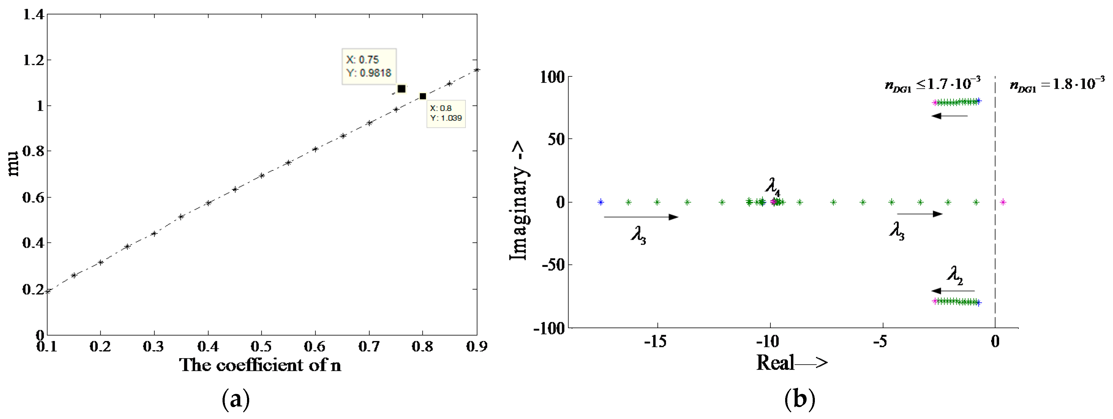
In this case, we assumed that the system in Figure 1 was subject to a single uncertainty parameter, i.e., parameter or , and the proposed method was employed to identify the stable boundary for each parameter of interest. It should be noted that the constraints on the parameters were considered, i.e., the values of and were limited by the rated active power ratio, , of DG1 to DG2. Similarly, the values of and were limited by the reactive rated power ratio, , of DG1 to DG2. Thus, the size coefficients of the two DG units were set to and . First, we considered the parameter to be the uncertainty in the MG. To illustrate the search process using the proposed method, the value of as a function of the size coefficient is plotted in Figure 13a, where , , and . As the size coefficient, , increased, the value of increased gradually and became close to 1, thereby indicating that the robust margin of the system was reduced. When the size factor, , had a value of 0.17, was able to reach 0.9629. As continued to increase by one step, the value of was 1.018, which showed that the system was unstable. Therefore, the maximum value of at which the system remained stable was 0.17. By substituting this value into Equation (3), we derived the upper bound of the frequency droop parameter as . Thus, the system is stable in the small-signal sense provided that the parameter is smaller than .
To verify the result, the eigenvalues were calculated for the MG system with the parameter, , under this stability range, and they are plotted in Figure 13b. The initial conditions of the system were the same as those described above. As shown, as parameter increased from to , some eigenvalues moved toward the unstable region, and only a few eigenvalues were far from the positive real axis. Clearly, all of the dominant eigenvalues fell into the left half plane. However, as the value of increased to , a pair of eigenvalues crossed the imaginary axis. Thus, the stability boundary of can be taken as , which is close to the computed boundary given in Figure 13a, although it is not equal.
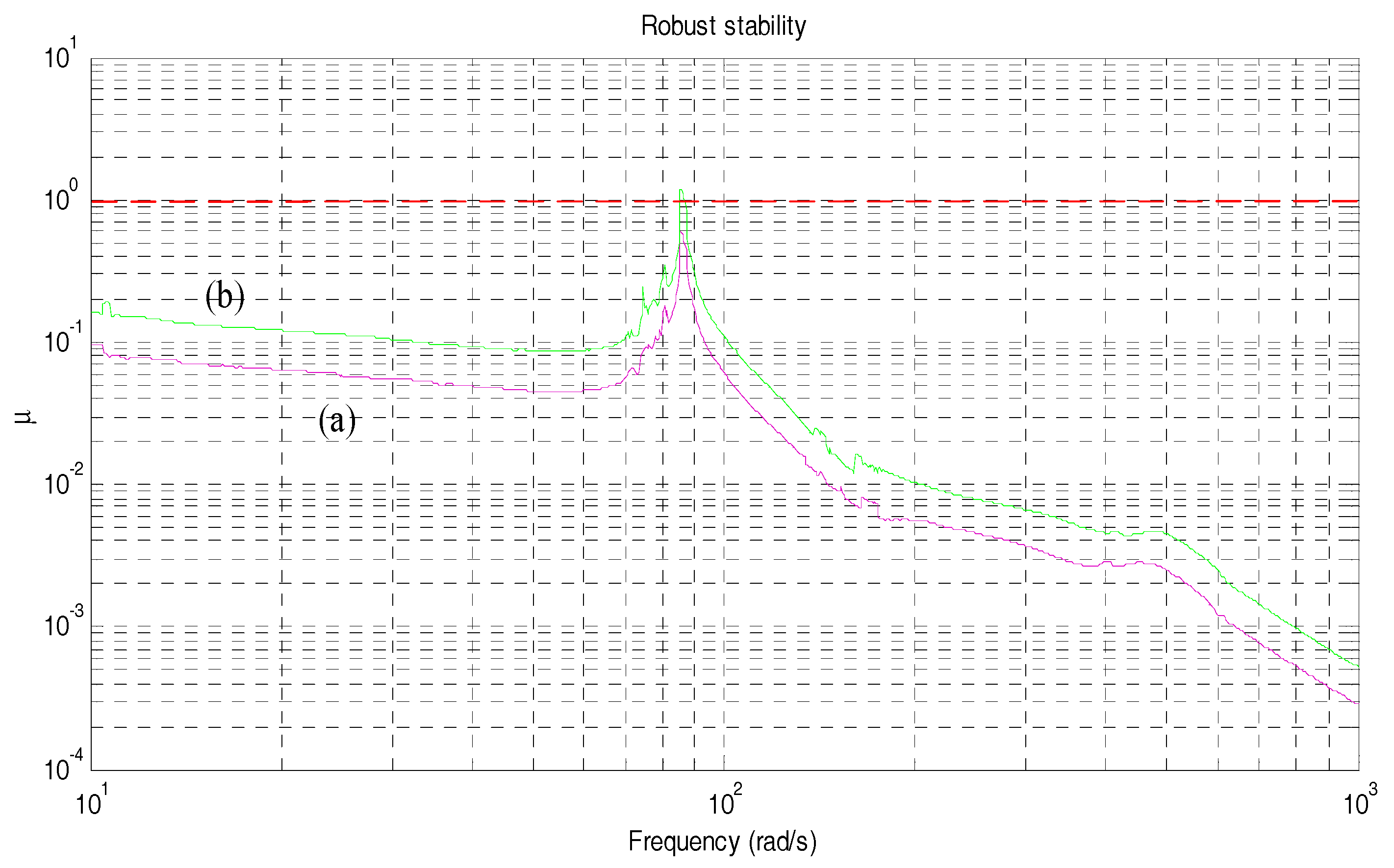
To further illustrate function , the frequency responses of were plotted by considering the droop parameters, , of 25.08 and 25.96. For the first value, was smaller than 1 for the entire frequency domain. In contrast, when parameter was set to 25.96, Figure 14 clearly shows that the maximum value of was 1.188 at a frequency of approximately 88 rad/s. Thus, the system was unstable under this value.
Next, we considered parameter as the uncertainty in the MG system. Figure 15a shows the trajectory of as a function of size coefficient . The initial values for and were and 0.1, respectively, and the step size, , was 0.05. As shown, using the maximum size factor, , the value of was smaller than 1 at 0.75. By substituting the value of into Equation (4), we derived the upper bound of the voltage droop parameter, , as .
In addition, we calculated the eigenvalues of the MG system with the parameter, , within this range to verify the result. Figure 15b shows the traces of the dominant eigenvalues when the voltage droop parameter, , varied from 0 to . When the droop parameter, , was not greater than , all of the dominant eigenvalues fell into the left half plane. An eigenvalue crossed the imaginary axis when the droop parameter, , was , which is close to the stability range obtained using the proposed method.
4.2. Case 2: Analysis of the Stability Range for Two Uncertainty Parameters
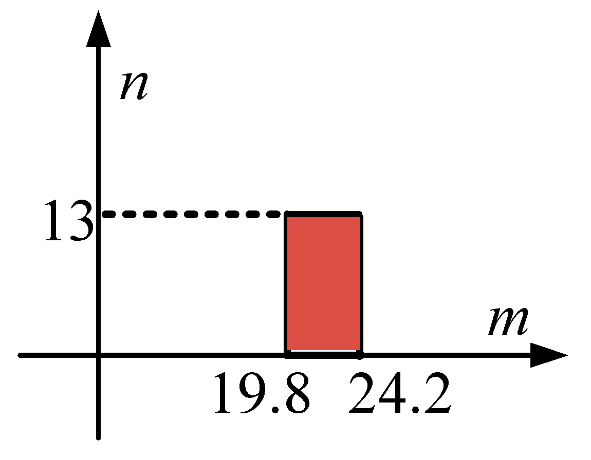
In this case, the system in Figure 1 was subject to simultaneous variations in two parameters, and . The proposed method was employed to identify the stable boundaries for these parameters. As explained previously, we first addressed the problem of how to obtain the stability boundary of uncertainty parameter when varied within a certain range. For example, the uncertainty parameter, , had an interval of ; then, using the proposed method, the stability boundary for parameter was determined as . Thus, the system is stable if is in the closed area shown in Figure 16.
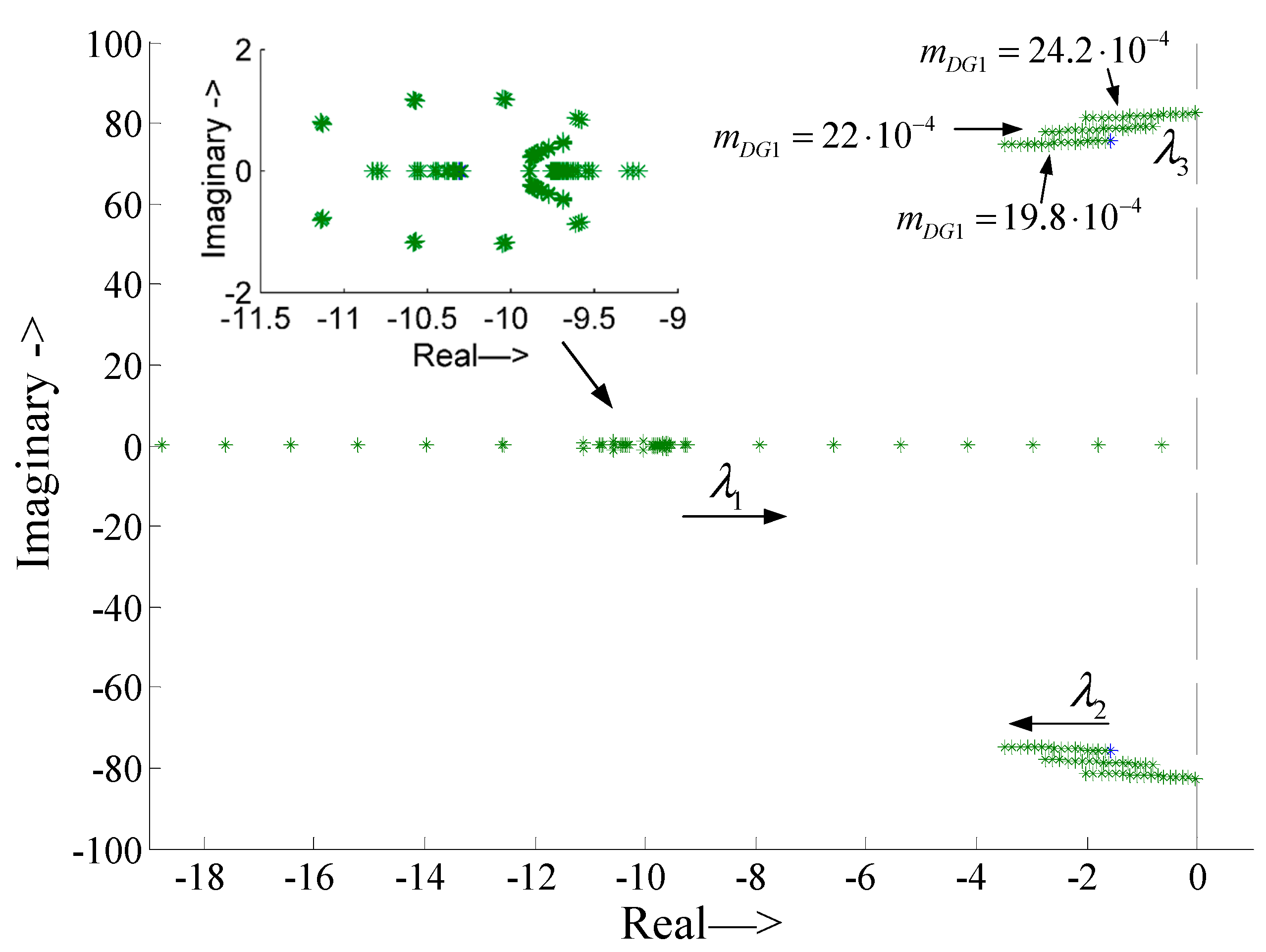
To verify the region obtained, we considered as many points as possible in this region and investigated the stability of the MG system at each point. Without any loss of generality, was set to , , or , and was taken as being within . The eigenvalues of an MG system considering such values are depicted in Figure 17, which demonstrates that the system remained stable when and were within this range. Outside this range, such as when the parameter increased slightly, an eigenvalue crossed the imaginary axis immediately. Similarly, when parameter increased slightly, a pair of eigenvalues moved to cross the imaginary axis.
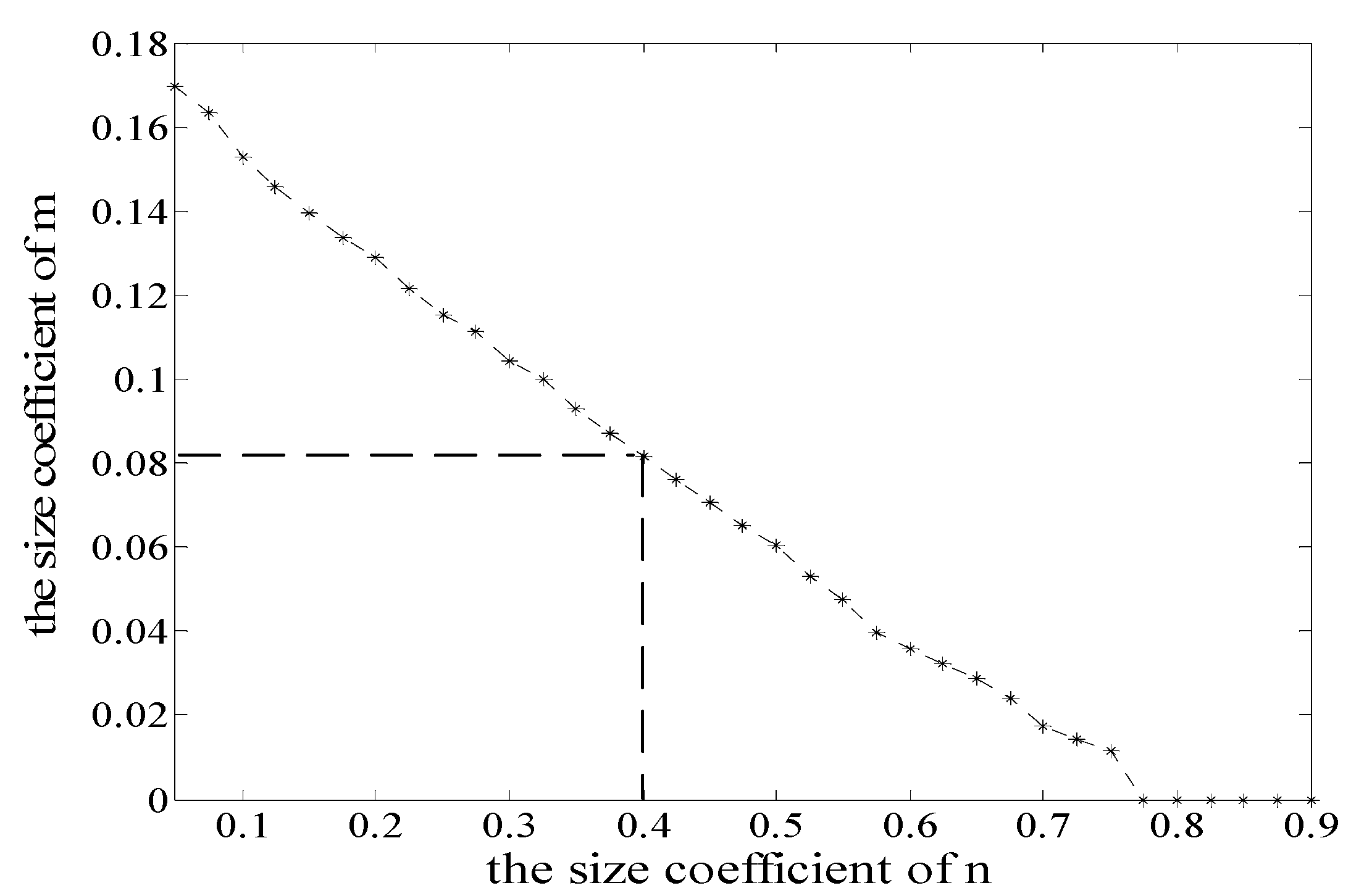
We then addressed the problem of the stability ranges for and . As explained previously, the stability ranges comprised multiple areas, as shown in Figure 10. To clearly illustrate the relationship between the stability boundaries of and , we employed the size coefficients and instead of and , respectively, to plot the stability range. Figure 18 shows the stability bounds for and , where each point on this black line represents the upper bound of parameter corresponding to each value of . For example, when the size coefficient, , had a value of about 0.08, the maximum size coefficient, , was 0.4. After converting these values to and using Equations (3) and (4), respectively, we found that when the uncertainty of parameter was smaller than , the system was stable provided that the uncertainty of parameter was smaller than .
5. Simulation Study
To further demonstrate the validity of the stability boundaries for the droop parameters, a model of the MG considered in this study was simulated with PSCAD/EMTDC software (Version:4.2.1, Manitoba HVDC Research Centre, Winnipeg, MB, Canada). A detailed illustration of the inverter circuit, pulse-width modulation (PWM) schemes, and power control is shown in Figure 1. The parameters and initial conditions for the system are listed in Table 1.
Two size coefficients for the droop parameters were selected from the values shown in Figure 18, and , which were in the stability range, and and , which were outside the range. The values of the size coefficients were converted into m and n using Equations (3) and (4), respectively.
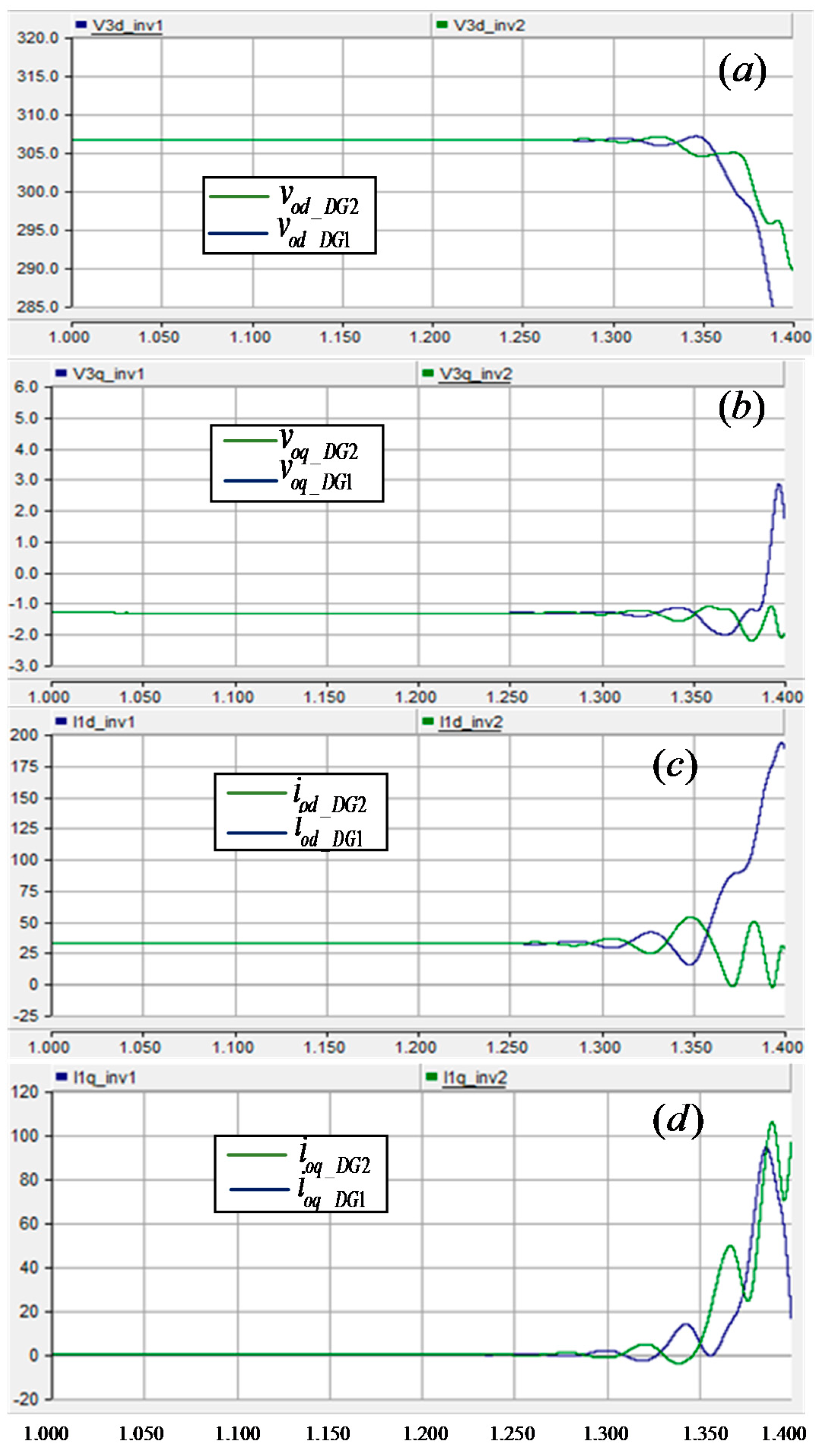
Figure 19 shows the dynamics of the output voltages and currents for the two sets of droop parameters. The system started from a steady state where the output currents and voltages for both DG1 and DG2 were close to constant. At s, the first set of data was assigned to and . After s, the other set of data was assigned. Figure 19 shows that the system remained stable for the first set of droop parameters. However, for data outside these points, the instantaneous currents and voltages oscillated for more than 10 cycles, and eventually became unstable. Therefore, the simulation results demonstrate the accuracy of the stability boundaries of the droop parameters predicted by analysis.
6. Conclusions
In this study, we addressed the problem of identifying the upper/lower bounds of uncertainty parameters in MGs. A novel approach was proposed based on analysis to solve this problem. The proposed general method is suitable for single and multiple uncertainty parameters. The accuracy of the proposed method was confirmed by the eigenvalue approach based on study cases. In addition, the proposed method is suitable when there are no constraints on the parameters, but also when constraints must be considered, thereby making it convenient for use in practical applications. Furthermore, based on the obtained region, it is also possible to estimate the stability margin for an MG in terms of the droop parameters, which is very useful for system designers. In future work, we will study the stability boundaries for droop parameters by considering changes in the load. This could further assist in the stable operation of MGs and enhance the utilization of renewable energy.
Author Contributions
This study was a collaborative effort among the authors. The authors contributed collectively to the theoretical analysis and preparation of the manuscript.
Acknowledgments
This study was supported by the National Natural Science Foundation of China (51277080) and the National Natural Science Foundation of China under Grant 51707069, the Ministry of Education Key Laboratory of Image Processing and Intelligence Control (IPIC2015-01), the State Key Laboratory of Alternate Electrical Power System with Renewable Energy Sources (LAPS18001), China Postdoctoral Science Foundation (2016M602296), and the Cultivation Foundation of Hubei Collaborative Innovation Center for High-Efficient Utilization of Solar Energy (HBSZD2014001).
Conflicts of Interest
The authors declare no conflicts of interest.
Appendix A
Figure 1 shows a schematic of the circuit of a DG unit, which comprises an ideal DC power, three-leg inverter, and an output LCL filter. Let and be the currents of inductance for and , respectively, and is the voltage of capacitance . The small-signal equations for the filter in the Park’s d–q frame are given by:
where , , , and are the variable values at the steady-state operating points. In this study, denotes a small variation in the equilibrium point values and represents the value of a variable at the steady-state operating points.
For the power controller, each DG unit shares the load in the MG by drooping the DG frequency in proportion to the power output. Let and be the output voltage and current of the DG unit, respectively. The instantaneous active output, ,and reactive power, , of the DG unit are calculated as follows:
Due to the effect of the harmonic component, and are passed through low-pass filters to obtain the fundamental component of power, where the dynamic filters can be described as follows:
where is the cut-off angular frequency of a low-pass filter.
Thus, the dynamics of the droop controller can be described as:
where and are the reference voltage and frequency, respectively. The small signal state spaces of Equations (A4)–(A6) are:
where is the angular frequency of the common reference frame. The angle between the individual reference frame and the common reference frame is represented by .
With respect to the voltage controller loop, the proportional-integral regulator is employed to follow the reference voltage. The small signal state spaces of this controller are given by:
where the introduced variable, , equals the integral of the difference between the reference voltage, , and measured voltage, . and are the coefficients of the proportional-integral regulator.
For the inner loop, the current controller uses the proportional regulator, and the dynamics of the controller are described as follows:
where is the coefficient of the proportion. We ignore the dynamic performance of the PWM of the inverter model, which is a standard assumption when considering the stability of an MG [31].
Appendix B
The network for the MG is shown in Figure 1. Let and be the current in the line and the output voltage of each node, respectively. The state equation for the network is as follows:
The system state matrices, , , and , are as follows:
where and are the resistor and inductor of the line, respectively.
In this study, only a general RL load is considered. The state equation for the RL load is as follows:
In Equation (A2),
where is the current of the load.
To connect each subsystem model for the MG, a virtual resistor, , is assumed between each node and the ground. Therefore, the voltage of each node is given by:
where , , .
Based on a common reference frame, the complete state-space small-signal model of the MG can be obtained by combining the state-space models of the DG with the RL load and network.
References
- Juan, M.C.; Leopoldo, G.F.; Jan, T.B.; Eduardo, G.; Ramón, C.P.; Prats, M.A.M.; José, I.L.; Narciso, M.A. Power electronic systems for the grid integration of renewable energy sources: A survey. IEEE Trans. Power Electron. 2006, 53, 1002–1016. [Google Scholar]
- Abdel-Rahim, N.M.; Quaicoe, J.E. Analysis and design of a multiple feedback loop control strategy for single-phase voltage-source UPS inverters. IEEE Trans. Power Electron. 1996, PE-11, 532–541. [Google Scholar] [CrossRef]
- Mohamed, Y.; El-Saadany, E. Adaptive decentralized droop controller to preserve power sharing stability of paralleled inverters in distributed generation microgrids. IEEE Trans. Power Electron. 2008, 23, 2806–2816. [Google Scholar] [CrossRef]
- Doyle, J. Analysis of feedback systems with structured uncertainties. IEE Proc. D (Control Theory Appl.) 1982, 129, 242–250. [Google Scholar] [CrossRef]
- Urquizo, J.; Calderón, C.; James, P. Using a local framework combining principal component regression and Monte Carlo simulation for uncertainty and sensitivity analysis of a domestic energy model in sub-city areas. Energies 2017, 10, 1986. [Google Scholar] [CrossRef]
- Zhou, K.; Doyle, J.; Glover, K. Robust and Optimal Control; Prentice Hall: Upper Saddle River, NJ, USA, 1996. [Google Scholar]
- Davari, M.; Mohamed, Y.A.R.I. Robust multi-objective control of VSC-based DC-voltage power port in hybrid AC/DC multi-terminal microgrids. IEEE Trans. Smart Grid 2013, 4, 1597–1612. [Google Scholar] [CrossRef]
- Coelho, E.A.A.; Cortizo, P.; Gracia, P.F.D. Small signal stability for parallel-connected inverters in stand-alone ac supply systems. IEEE Trans. Ind. Appl. 2002, 38, 533–542. [Google Scholar] [CrossRef]
- Pogaku, N.; Prodanovic, M.; Green, T.C.; Kling, W.L.; van der Sluis, L. Modeling analysis and testing of autonomous operation of an inverter-based microgrid. IEEE Trans. Power Electron. 2007, 22, 613–625. [Google Scholar] [CrossRef]
- Yang, L.; Xu, Z.; Østergaard, J.; Dong, Z.Y.; Wong, K.; Ma, X. Oscillatory stability and eigen value sensitivity analysis of a DFIG wind turbine system. IEEE Trans. Energy Convers. 2011, 26, 328–339. [Google Scholar] [CrossRef] [Green Version]
- Katiraei, F.; Iravani, M.R.; Lehn, P.W. Small-signal dynamic model of a microgrid including conventional and electronically interfaced distributed resources. IET Gener. Transm. Distrib. 2007, 1, 369–378. [Google Scholar] [CrossRef]
- Riccobono, A.; Santi, E. Comprehensive review of stability criteria for DC power distribution systems. IEEE Trans. Ind. Appl. 2014, 50, 3525–3535. [Google Scholar] [CrossRef]
- Sun, J. Impedance-based stability criterion for grid-connected inverters. IEEE Trans. Power Electron. 2011, 26, 3075–3078. [Google Scholar] [CrossRef]
- Feng, X.; Liu, J.; Lee, F.C. Impedance specifications for stable DC distributed power systems. IEEE Trans. Power Electron. 2002, 17, 157–168. [Google Scholar] [CrossRef]
- Riccobono, A.; Santi, E. A novel Passivity-Based Stability Criterion (PBSC) for switching converter DC distribution systems. In Proceedings of the 27th IEEE Annual IEEE Applied Power Electronics Conference and Exposition, Orlando, FL, USA, 5–9 February 2012; pp. 2560–2567. [Google Scholar]
- Castellanos, R.; Messina, A.; Sarmiento, H. Robust stability analysis of large power systems using the structured singular value theory. Int. J. Electr. Power Energy Syst. 2005, 27, 389–397. [Google Scholar] [CrossRef]
- Sumsurooah, S.; Odavic, M.; Bozhko, S. A modeling methodology for robust stability analysis of nonlinear electrical power systems under parameter uncertainties. IEEE Trans. Ind. Appl. 2016, 52, 4416–4425. [Google Scholar] [CrossRef]
- Salis, V.; Costabeber, A.; Cox, S.M.; Zanchetta, P.; Formentini, A. Stability boundary analysis in single-phase grid-connected inverters with PLL by TLP theory. IEEE Trans. Power Electron. 2017, 33, 4023–4036. [Google Scholar] [CrossRef]
- Zheng, J.H.; Wang, Y.; Wang, Z.; Zhu, S.; Wang, X.; Xinwei, S. Study on microgrid operation modes switching based on eigenvalue analysis. APAP 2011, 1, 445–450. [Google Scholar]
- Haddadi, A. A μ-based approach to small-signal stability analysis of an interconnected distributed energy resource unit and load. IEEE Trans. Power Deliv. 2015, 30, 1715–1726. [Google Scholar] [CrossRef]
- Guerrero, J.M.; Vicuna, L.G.; Matas, J.; Castilla, M.; Miret, J. A wireless controller to enhance dynamic performance of parallel inverters in distributed generation systems. IEEE Trans. Power. Electron. 2004, 19, 1205–1213. [Google Scholar] [CrossRef]
- Alvarado, F.L. Bifurcations in nonlinear systems: Computational issues. In Proceedings of the International Symposium on Circuits and Systems (ISCAS), New Orleans, LA, USA, 29 April–3 May 1990. [Google Scholar]
- Hill, D. Nonlinear computation and control for small disturbance stability. In Proceedings of the IEEE Summer Meeting, Seattle, WA, USA, 16–20 July 2000. [Google Scholar]
- De Souza, A.C.Z. Tangent vector applied to voltage collapse and loss sensitivity studies. Electr. Power Syst. Res. 1998, 47, 65–70. [Google Scholar] [CrossRef]
- Tiranuchit, A.; Thomas, R. A posturing strategy against voltage instabilities in electric power systems. IEEE Trans. Power Syst. 1988, 3, 87–93. [Google Scholar] [CrossRef]
- Yorino, N.; Li, H.-Q.; Sasaki, H. A predictor/corrector scheme for obtaining q-limit points for power flow studies. IEEE Trans. Power Syst. 2005, 20, 130–137. [Google Scholar] [CrossRef]
- Rommes, J.; Martins, N. Computing large-scale system eigenvalues most sensitive to parameter changes, with applications to power system small-signal stability. IEEE Trans. Power Syst. 2008, 23, 434–442. [Google Scholar] [CrossRef]
- Luo, C.; Ajjarapu, V. Sensitivity-based efficient identification of oscillatory stability margin and damping margin using continuation of invariant subspaces. IEEE Trans. Power Syst. 2011, 26, 1484–1492. [Google Scholar] [CrossRef]
- Yang, D.; Ajjarapu, V. Critical eigenvalues tracing for power system analysis via continuation of invariant subspaces and projected Arnoldi method. IEEE Trans. Power Syst. 2007, 22, 324–332. [Google Scholar] [CrossRef]
- Wang, Y.; Wang, J.; Zeng, W.; Liu, H.; Chai, Y. H Robust control of an LCL-type Grid-connected inverter with large-scale grid impedance perturbation. Energies 2018, 11, 57. [Google Scholar] [CrossRef]
- Li, Y.W.; Vilathgamuwa, D.M.; Loh, P.C. Design analysis and real-time testing of a controller for multibus microgrid system. IEEE Trans. Power Electron. 2004, 19, 1195–1204. [Google Scholar] [CrossRef]
- Doyle, J.C.; Wall, J.C.; Stein, G. Performance and robustness analysis for structured uncertainty. In Proceedings of the 21st IEEE Conference on Decision and Control, Orlando, FL, USA, 8–10 December 1982. [Google Scholar]
- Shah, S.; Sensarma, P.S. Three degree of freedom robust voltage controller for instantaneous current sharing among voltage source inverters in parallel. IEEE Trans. Power Electron. 2010, 25, 3003–3014. [Google Scholar] [CrossRef]
Figure 1.
Structure and control structure for a microgrid (MG). IBS: intelligent bypass switch; PWM: Pulse-Width Modulation; PLL: Phase Locking Loop.
Figure 1.
Structure and control structure for a microgrid (MG). IBS: intelligent bypass switch; PWM: Pulse-Width Modulation; PLL: Phase Locking Loop.

Figure 2.
Analogue block diagram of a distributed generation (DG) unit and its controller.

Figure 3.
Trace of dominant eigenvalue with increasing the frequency droop gain of both DG1 and DG2 units.
Figure 3.
Trace of dominant eigenvalue with increasing the frequency droop gain of both DG1 and DG2 units.

Figure 4.
Standard configuration of a system with perturbations.

Figure 5.
Representation of droop parameters as the linear fractional transformation (LFT) configuration.
Figure 5.
Representation of droop parameters as the linear fractional transformation (LFT) configuration.

Figure 6.
LFT configuration of a DG unit.

Figure 7.
Block diagram of the complete state-space model of a MG.

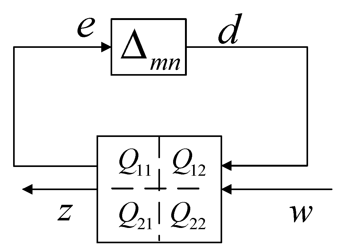
Figure 8.
configuration of a MG with uncertainty parameters.

Figure 9.
Process employed to identify the upper/lower bounds of a single uncertainty parameter. (a) finding a boundary for an uncertainty parameter and determining its type; (b) searching for the lower bound; (c) searching for the upper bound.
Figure 9.
Process employed to identify the upper/lower bounds of a single uncertainty parameter. (a) finding a boundary for an uncertainty parameter and determining its type; (b) searching for the lower bound; (c) searching for the upper bound.

Figure 10.
Stability boundaries of two uncertainty parameters.

Figure 11.
Algorithm for identifying the bounds of multiple uncertainty parameters.

Figure 12.
Process employed to search for the upper/lower bounds of uncertainty parameter when is in the range of . (a) Finding a boundary for an uncertainty parameter and determining its type; (b) Searching for the lower bound; (c) Searching for the upper bound.
Figure 12.
Process employed to search for the upper/lower bounds of uncertainty parameter when is in the range of . (a) Finding a boundary for an uncertainty parameter and determining its type; (b) Searching for the lower bound; (c) Searching for the upper bound.

Figure 13.
(a) Value of for size coefficients and ; (b) dominant eigenvalues for the MG with and .

Figure 14.
Frequency responses of for the MG with size coefficients of (a) and (b) .

Figure 15.
(a) Value of with size coefficients and . (b) Dominant eigenvalues for the MG with and .

Figure 16.
The stable region for droop parameters in the MG.

Figure 17.
Dominant eigenvalues of a MG when , .

Figure 18.
The stable region for size coefficients and .

Figure 19.
Response of the DG unit with two sets of droop parameters: (a) d-axis components of the output voltage, ; (b) q-axis components of the output voltage, ; (c) d-axis components of the output current, ; and (d) q-axis components of the output current, .
Figure 19.
Response of the DG unit with two sets of droop parameters: (a) d-axis components of the output voltage, ; (b) q-axis components of the output voltage, ; (c) d-axis components of the output current, ; and (d) q-axis components of the output current, .


Table 1.
Microgrid (MG) Parameters.
| Parameter | Symbol | Value |
|---|---|---|
| Inverter switching frequency | 5 kHz | |
| Filter inductance | 1.5 mH | |
| Parasitic resistor | 0.001 | |
| Filter capacitance | 102 μF | |
| Filter inductance | 0.53 mH | |
| Parasitic resistor | 0.05 | |
| Rating of output voltage | 311 V | |
| Nominal frequency | 50 Hz | |
| droop | ||
| droop | ||
| Parameters for lines 1 and 2 | 0.1 | |
| 1.12 mH | ||
| Load parameters | 4.279 | |
| 2.94 mH |
© 2018 by the authors. Licensee MDPI, Basel, Switzerland. This article is an open access article distributed under the terms and conditions of the Creative Commons Attribution (CC BY) license (http://creativecommons.org/licenses/by/4.0/).
Share and Cite
MDPI and ACS Style
Ding, X.; Li, K.; Li, Y.; Cai, D.; Luo, Y.; Dong, Y. A Novel Approach for Searching the Upper/Lower Bounds of Uncertainty Parameters in Microgrids. Energies 2018, 11, 1035. https://doi.org/10.3390/en11051035
AMA Style
Ding X, Li K, Li Y, Cai D, Luo Y, Dong Y. A Novel Approach for Searching the Upper/Lower Bounds of Uncertainty Parameters in Microgrids. Energies. 2018; 11(5):1035. https://doi.org/10.3390/en11051035
Chicago/Turabian StyleDing, Xiaojun, Kaicheng Li, Yuanzheng Li, Delong Cai, Yi Luo, and Youli Dong. 2018. "A Novel Approach for Searching the Upper/Lower Bounds of Uncertainty Parameters in Microgrids" Energies 11, no. 5: 1035. https://doi.org/10.3390/en11051035
Note that from the first issue of 2016, this journal uses article numbers instead of page numbers. See further details here.