Design Methods of Underwater Grounding Electrode Array by Considering Inter-Electrode Interference for Floating PVs

Abstract

An optimal design method is proposed in this paper to improve the safety and price competitiveness of floating photovoltaic (PV) systems. From the standards for grounding by the International Electrotechnical Commission (IEC) 60364, the Electrical Equipment Technology Standards (EETS) are set up for the grounding resistance to be less than or equal to 10 $\mathsf{\Omega }$ for high voltage (above 750 V DC) and extra high voltage (above 7000 V) systems. In order to satisfy this criterion, a parallel connection of grounding electrodes is essential in the system. Furthermore, inter-electrode interference should be considered to reflect the resistance increase due to the potential increase between electrodes. Therefore, in this study, the parallel grounding resistance according to the distance and number of electrodes, as well as the arrangement method were theoretically predicted and compared with the measured values. For the first time, the design of grounding electrodes has been applied to real floating PV systems and is expected to satisfy EETS.

1. Introduction

As fossil energy depletion and environmental problems increase, interest in new and renewable energy is increasing [1,2,3]. Solar energy accounts for a large proportion of the new and renewable energy sources [4,5]. Currently, large-scale photovoltaic (PV) plants are continuously being installed [6,7,8,9,10]. In addition, policies such as the Renewable Portfolio Standards (RPS) in the United States of America [11,12,13], Renewable Obligations (RO) in the United Kingdom [14,15] and Renewable Purchase Obligation (RPO) in India [16,17] encourage the expansion of PV generation [18,19,20]. In Korea, the government is trying to increase solar energy by announcing the Renewable Energy 3020 Implementation Plan [21]. This plan includes increasing the proportion of renewable energy generation by 20% by 2030. However, due to limited land area, it is not easy to secure PV plant sites [22]. Therefore, installation of PV systems of 3000 kW or less on rooftops or on the surfaces of bodies of water is recommended by awarding a Renewable Energy Certificate (REC) 1.5 supply certificate [23]. REC is a kind of incentive for renewable energy generation in order to promote the spread of renewable energy. In other words, the electricity generated from the photovoltaic module on the water could be sold by multiplying the weight by 1.5-times the existing price.

In particular, a PV system in which the PV module is installed on a water surface using a buoyant body is called a floating PV system [24,25]. Floating PV systems are being installed using idle water worldwide. Currently, the largest floating PV plant of 150 MW is being installed in Anhui, China. In addition, Korea is installing a total of 280 MW worth of floating PV plants: 100 MW on Seongmin Lake, 100 MW on Daeho Lake and 80 MW on Goheung Lake. However, because floating PV systems require a buoyant structure that can operate stably even in unstable environments, such as during the flood season and typhoons [26,27], the power generation cost is higher than that of PV systems installed on land [28]. Therefore, many research institutions are conducting research on floating PV systems and developing technologies to reduce the unit cost [26,27,29]. As with PV systems installed on land, floating PV systems require grounding facilities to prevent damage from lightning or leakage current. Globally, the standards for grounding are established by the International Electrotechnical Commission (IEC). Ground provisions are detailed in IEC 60364 [30]. In Korea, the grounding method is based on the Electric Equipment Technical Standards, which require that grounding resistance should be less than or equal to 100 $\mathsf{\Omega }$ for low voltages and that grounding resistance should be less than or equal to 10 $\mathsf{\Omega }$ for systems above 400 V DC, high voltage and extra high voltage [31]. However, there is no standard grounding method suitable for floating PV systems. On the one hand, in shallow water, like reservoirs and lakes, grounding lines could be dragged onto land. On the other hand, in deep water, such as lakes and dams, it is not easy to install a grounding line on the bottom due to cost problems compared to land PV systems. Thus, in this study, the arrangement method of grounding electrodes for safety in floating PV systems was analyzed using the underwater grounding method, in which the grounding electrode is directly grounded in water to reduce the unit cost of the floating PV system, as shown in Figure 1.

Recently, a study on the design of underwater grounding has been published [32], but subsequent research is still needed. In Korea, in the case of a PV power plant, it is necessary that the grounding resistance be less than or equal to 10 $\mathsf{\Omega }$. However, it is difficult to meet this criterion using a single grounding electrode. Therefore, multiple grounding electrodes should be connected in parallel and grounded. When multiple grounding electrodes are connected in parallel, the grounding resistance increases from the ideal value (the value obtained by dividing the resistance of one grounding electrode by the number of electrodes) due to the potential rise from the mutual electrode interference [33]. The potential to be increased depends on the length of the grounding electrode, the number of grounding electrodes and the distance between the grounding electrodes. Therefore, in this paper, the arrangement method of parallel grounding electrodes was analyzed considering these factors. Experiments were carried out at the floating PV system in Hapcheon Dam, Korea, where the depth is approximately 40 m.

2. Single Grounding Resistance Design

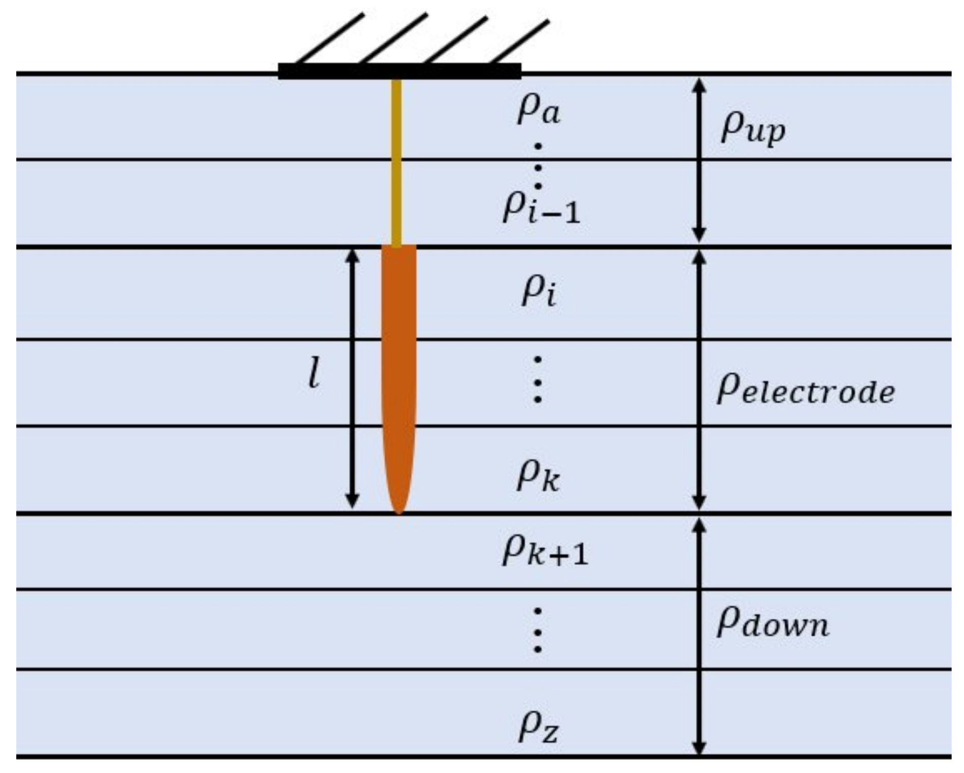
2.1. Modeling of Underwater Grounding Resistance

The underwater region is a structure divided into multiple layers of water with different resistivities. Therefore, the total grounding resistance can be regarded as a form in which the resistances with different resistivity are connected in parallel [32]. Each section of water can be roughly divided into three parts: the part between the water surface and the top of the grounding electrode (${\rho }_{up}$), the part where the electrode contacts the water (${\rho }_{electrode}$) and the part between the end of the grounding electrode and the bottom (${\rho }_{down}$), as shown in Figure 2. The total water resistivity (${\rho }_{total}$) can be expressed as the sum of the resistivity of each layer, as shown in Equation (1).

$$\begin{array}{cc}\hfill {\rho }_{total}& ={\rho }_{up}+{\rho }_{electrode}+{\rho }_{down}\hfill \\ & =\frac{{\sum }_{x=a}^{i-1}{h}_x}{{\sum }_{x=a}^{i-1}\frac{h_x}{{\rho }_x}}+\frac{l}{{\sum }_{x=i}^{k-1}\frac{h_x}{{\rho }_x}+\frac{l-{\sum }_{x=i}^{k-1}{h}_x}{{\rho }_x}}+\frac{{\sum }_{x=k+1}^z{h}_x}{{\sum }_{x=k+1}^z\frac{h_x}{{\rho }_x}}\hfill \end{array}$$

(1)

In Equation (1), l is the length of the grounding electrode, $h_x$ is the distance between layers and ${\rho }_x$ is the resistivity of each layer. The grounding electrode used in the experiment is a rod-shaped electrode made of copper. The total grounding resistance can be expressed as Equation (2) [34].

$$R=\frac{{\rho }_{total}}{2\pi l}ln\frac{2l}{d}$$

(2)

In Equation (2), l is the length of the grounding electrode and d is the radius of the grounding electrode. As can be seen from Equation (2), the grounding resistance varies with the length of the grounding electrode. Moreover, the resistivity of the water can vary greatly depending on the water temperature and the amount of organic matter present [35].

$${\rho }_T=\frac{1}{{\sigma }_T}=\frac{1}{{\sigma }_{25{ }^{°}\mathrm{C}}\left[1+\alpha \left(T-25{ }^{°}\mathrm{C}\right)\right]}$$

(3)

Equation (3) shows the relationship between resistivity and water temperature. $\alpha$ is the temperature coefficient of electrical conductivity, which increases linearly as water temperature increases. In other words, the grounding resistance tends to decrease as the temperature increases. Therefore, for accurate prediction of underwater grounding resistance, the effects of grounding electrode length, water temperature, installation depth and season should be considered.

2.2. Single Grounding Resistance Design

Because the length and diameter of the grounding electrode have a large effect on the single grounding resistance value, a rod-shaped copper grounding electrode with a length of 1.8 m and a diameter of 16 mm was compared with a rod-shaped copper grounding electrode with a length of 0.5 m and a diameter of 12 mm. Figure 3 shows the variation in the water temperature of the dam (15 January, 15 April, 15 July, 15 October 2015) at the depth of Hapcheon. The floating PV system in Hapcheon Dam has a depth of approximately 40 m, so the temperature difference between the water surface and the bottom is considerably large, especially in summer and autumn. Therefore, the resistivity difference between the water surface and the bottom is large.

Figure 4 shows the change in the resistance of the 1.8-m copper electrode and 0.5-m copper electrode due to water depth measured in the spring of 2016 [32]. In both grounding electrodes, the resistance increases as the water depth increases, due to decreasing temperature. An exception to this trend is from the surface of the water to a depth of 5 m, where the resistance decreases with depth, which is presumed to be due to the different amount of organic matter at this water depth. Because the resistance becomes smaller at up to 5 m of depth, the installation depth of the grounding electrode should be within 5 m. The minimum installation underwater thickness of the electrode, however, should be placed deeper than the ice thickness to protect against the sharp increase of the resistance due to the resistivity of the ice.

Figure 5 shows the variation in the single grounding resistance of copper and stainless-steel installed at Hapcheon Dam and Sangju Otae Reservoir every three months from September 2016 to December 2017. Unlike Hapcheon Dam, the water depth in Sangju Otae reservoir is as low as 3 m. In order to compare the degree of corrosion over time, a stainless-steel grounding rod with relatively low corrosion was also installed. The copper electrode was a 1.8-m long, 16-mm diameter grounding rod, and the stainless-steel electrode was a 1.2-m, 28-mm diameter grounding rod. As a result, the lowest water temperature drops to 6 ${}^{\circ }$C, and the resistance of the copper electrode shows a difference of approximately 30 $\mathsf{\Omega }$, according to the water temperature. In addition, a comparison was attempted between the degree of corrosion of the stainless-steel grounding electrode and that of the copper grounding electrode, but it was difficult to confirm the effect of corrosion because the degree of corrosion measured within one year and three months was within the measurement error range.

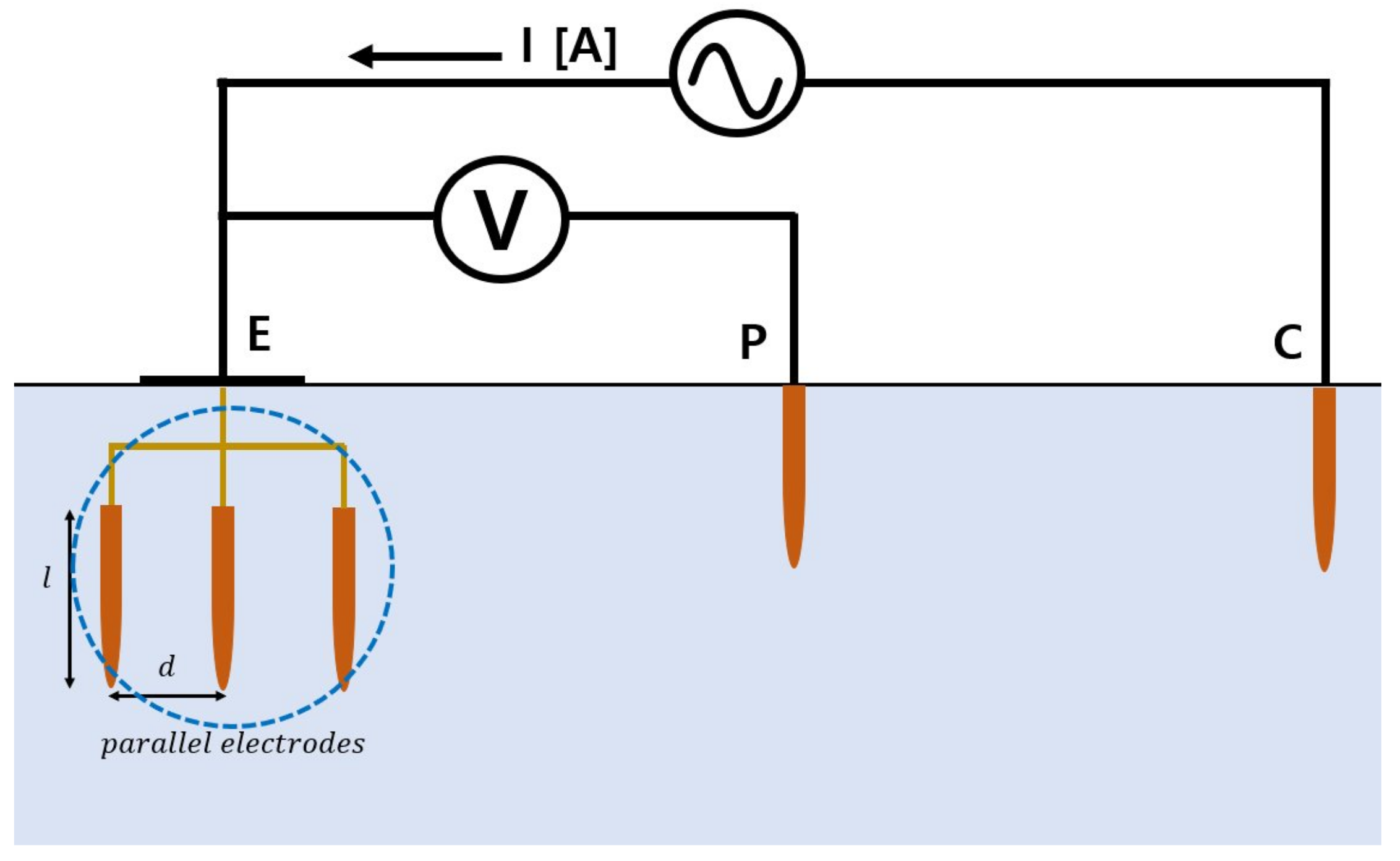
2.3. Parallel Grounding Resistance Design

In the case of a PV power plant, it is necessary that the grounding resistance be less than or equal to 10 $\mathsf{\Omega }$, but it is difficult to meet this criterion using a single grounding electrode. Therefore, multiple grounding electrodes should be connected in parallel and grounded. The total grounding resistance (R) due to the parallel connection of the grounding electrode is expressed as Equation (4) [36].

$$R=\eta \frac{R_0}{n}$$

(4)

$R_0$ is a single grounding resistance; n is the number of grounding electrodes; and $\eta$ is the coefficient of parallel connection. Ideally, the coefficient of parallel connection should be one, but because the distance between electrodes is not infinite, it is greater than one because of the mutual interference of the parallel electrodes. Therefore, when the grounding electrodes are connected in parallel, it is necessary to predict the coefficient of parallel connection to accurately predict the total grounding resistance. Figure 6 shows the measured total grounding resistance and coefficient of parallel connection, which changes according to the electrode gap and season, when two 0.5-m grounding electrodes were installed at a 1-m depth in the floating PV system of Hapcheon Dam.

In this experiment, the fall-of-potential method was used to measure parallel grounding resistance, as shown in Figure 7. In Figure 7, E represents the parallel electrodes and P is the auxiliary electrode used to measure the potential difference at E. C is the auxiliary electrode used to apply a current. In this method, the potential difference between P and C is assumed to be zero by providing a sufficient distance from E. The grounding resistance could be determined by the current flowing from the power source to water and the potential difference between E and P.

The coefficient of parallel connection is the largest in December with the lowest water temperature and the smallest is in July with the highest water temperature. It can also be seen that as the distance between the grounding electrodes becomes larger, the coefficient of parallel connection decreases, and when the distance between the electrodes becomes approximately 10 m, it becomes close to one, which is the ideal value. However, it is difficult to comply with the requirement that grounding resistance should be less than or equal to 10 $\mathsf{\Omega }$ with only two grounding electrodes. Therefore, the variation in the coefficient of parallel connection was measured by increasing the number of grounding electrodes. Figure 8 shows the coefficient of parallel connection with a length of 0.5 m while changing the distance between the grounding electrodes and the number of grounding electrodes.

As shown in Figure 8, as the number of grounding electrodes increases, the coefficient of parallel connection increases linearly. That is, as the number of the grounding electrodes increases, the mutual interference between the grounding electrodes increases, and the grounding resistance increases as the distance between the grounding electrodes decreases. Because of the limit of the wire length used in the experiment, the maximum gap of two electrodes is 18 m; the maximum gap of three electrodes is 8 m; the maximum gap of four electrodes is 5 m; and the maximum gap of five electrodes is 3 m.

2.4. Arrangement Method of Grounding Electrodes in Floating PV Systems

As the number of grounding electrodes increases, the value of the grounding resistance may vary depending on how the grounding electrode is disposed. For economic reasons, the number of grounding electrodes should be minimized. In order to reduce the number of grounding electrodes, it is necessary to reduce the mutual interference between the grounding electrodes by increasing the interval among the grounding electrodes. There are three types of arrangements in which the spacing between the grounding electrodes is minimized: linear, quadrangle or ring types. Ideally, all the grounding electrodes should be installed in a linear configuration to minimize the inter-electrode interference between the grounding electrodes, but it may be difficult to install them in a linear manner because of the conditions of the floating PV system. To compare the required area and maximum distance of each arrangement type, the distance between the electrodes is defined as d, and the number of grounding electrodes to be installed is defined as n. A comparison of the arrangements of electrodes is shown in

Table 1. Comparison of the arrangement of electrode.

Type	Arrangement	Maximum Distance	Required Area
Linear		$(n-1)d$	$(n-1)d$
Quadrangle		$\sqrt{2}d\left(1<n\le 4\right)$ $2\sqrt{2}d\left(4<n\le 8\right)$ ⋮	$\frac{d}{sin({180}^{\circ }/n)}$
Ring		$d^2\left(1<n\le 4\right)$ ${4d}^2\left(4<n\le 8\right)$ ⋮	$\frac{n{d}^2}{4tan({180}^{\circ }/n)}$

.

Based on both the required area and the maximum distance, the quadrangle type is most effective. In order to calculate the parallel grounding resistance according to the arrangement type, the influence of interference between each grounding electrode should be considered. For the calculation of parallel grounding resistance, the arrangement of grounding electrodes is assumed to be an (n × n) matrix. The general formula for grounding resistance is shown in Equation (5) [37].

$$V\left(x\right)=\rho ·F\left(x\right)·I$$

(5)

In Equation (5), I is the grounding current, $V\left(x\right)$ is the potential generated when I flows and $F\left(x\right)$ is a function related to the radius or distance of the grounding electrodes. $\rho$ is the earth resistivity, and in this paper, it refers to the resistivity of water. When the grounding electrodes are installed, each installation point is called $p_1$, $p_2$, ⋯,$p_n$, and points $p_1$($x_1$ , $y_1$), $p_2$ ($x_2$ , $y_2$), ⋯, $p_n$ ($x_n$ , $y_n$) are assigned to each installation point based on an arbitrary point ($p_1$). The rise in the potential of the k-th electrode is the sum of the potential rise of the k-th electrode and the potential rise of other electrodes, as shown in Equation (6).

$$V_k=\sum _{i=1}^{k-1}\rho F\left(S_{ik}\right)I_i+\rho R_f{I}_k+\sum _{i=k+1}^n\rho F\left(S_{ik}\right)I_i$$

(6)

In Equation (6), $S_{ik}$ denotes the distance between the i-th grounding electrode and k-th grounding electrode. On the right, the second term represents the potential rise by the same electrode. The first and third terms represent the potential rise by other electrodes. $R_f$ is $\frac{R}{{\rho }_{total}}$, which is related to the length and radius of the grounding electrode. Equation (6) can be expressed by a matrix, as Equation (7).

$$\begin{array}{cc}\hfill V& =\rho FI\hfill \\ \hfill \mathrm{where}:V=\left[\begin{array}{c}{V}_1\\ V_2\\ ⋮\\ V_n\end{array}\right],I& =\left[\begin{array}{cccc}{I}_1& I_2& \cdots & I_n\end{array}\right],F=\left[\begin{array}{cccc}{R}_f& F\left(S_{12}\right)& \cdots & F\left(S_{1n}\right)\\ F\left(S_{21}\right)& R_f& \cdots & F\left(S_{2n}\right)\\ ⋮& & \ddots & ⋮\\ F\left(S_{n1}\right)& \cdots & \cdots & R_f\end{array}\right]\hfill \end{array}$$

(7)

$V_n$ and $I_n$ denote the potential and current of the n-th grounding electrode, respectively. In this paper, it is assumed that the potentials of all the electrodes are the same, because all the grounding electrodes have the same length and diameter.

$$V=\left[\begin{array}{c}{V}_1\\ V_2\\ ⋮\\ V_n\end{array}\right]=V\left[\begin{array}{c}1\\ 1\\ ⋮\\ 1\end{array}\right]$$

(8)

Furthermore, the total grounding current can be expressed as the sum of the currents of the grounding electrodes, as shown in Equation (9).

$$I=I_1+I_2+\cdots I_n=I\left[\begin{array}{cccc}1& 1& \cdots & 1\end{array}\right]$$

(9)

Equation (5) can be summarized as shown in Equation (10).

$$I=\frac{1}{\rho }{F}^{-1}V$$

(10)

The parallel grounding resistance is the ratio of the electrode potential to the grounding current. Therefore, the parallel grounding resistance can be expressed as Equation (11).

$$R=\frac{V}{I}=\frac{\rho }{\left[\begin{array}{cccc}1& 1& \cdots & 1\end{array}\right]F^{-1}\left[\begin{array}{c}1\\ 1\\ ⋮\\ 1\end{array}\right]}$$

(11)

In order to calculate the parallel grounding resistance of the rod-shaped electrode, the equation for calculating the potential distribution of the electrode must first be obtained as shown in Equation (12).

$$\begin{array}{cc}\hfill V\left(x\right)& =\frac{\rho I}{4\pi kl}ln\frac{1+e}{1-e}\hfill \\ \hfill \mathrm{where},k& =\sqrt{1-\frac{r^2}{l^2}},e=\sqrt{1-\frac{x^2}{l^2+x^2-r^2}}\hfill \end{array}$$

(12)

In Figure 9, r is the radius of the grounding electrode and l is the length of the grounding electrode. When two grounding electrodes are connected in parallel, Equations (7) and (12) can be used as shown in Equation (13).

$$\begin{array}{cc}\hfill \left[\begin{array}{c}{V}_1\\ V_2\end{array}\right]& =\frac{\rho }{4\pi kl}\left[\begin{array}{cc}f\left(r\right)& f\left(S\right)\\ f\left(S\right)& f\left(r\right)\end{array}\right]\left[\begin{array}{c}{I}_1\\ I_2\end{array}\right]\hfill \\ \hfill \mathrm{where},f\left(x\right)& =ln\frac{1+e}{1-e}\hfill \end{array}$$

(13)

Equation (13) is summarized by the equation of current shown in Equation (14).

$$\left[\begin{array}{c}{I}_1\\ I_2\end{array}\right]=\frac{4\pi kl}{\rho }{\left[\begin{array}{cc}f\left(r\right)& f\left(S\right)\\ f\left(S\right)& f\left(r\right)\end{array}\right]}^{-1}\left[\begin{array}{c}{V}_1\\ V_2\end{array}\right]=\frac{4\pi kl}{\rho (f{\left(r\right)}^2-f{\left(S\right)}^2)}\left[\begin{array}{cc}f\left(r\right)& -f\left(S\right)\\ -f\left(S\right)& f\left(r\right)\end{array}\right]\left[\begin{array}{c}{V}_1\\ V_2\end{array}\right]$$

(14)

As the grounding current is the sum of each current, the grounding current is given by Equation (15).

$$I=\frac{4\pi kl}{\rho (f{\left(r\right)}^2-f{\left(S\right)}^2)}(2f\left(r\right)-2f\left(S\right))V$$

(15)

Equation (15) can be expressed as the ratio of the potential to the grounding current, and the parallel grounding resistance of two grounding electrodes can be obtained as shown in Equation (16).

$$R=\frac{V}{I}=\frac{\rho (f{\left(r\right)}^2-f{\left(S\right)}^2)}{4\pi kl\left(2f\right(r)-2f(S\left)\right)}=\frac{\rho \left(f\right(r)+f(S\left)\right)}{8\pi kl}$$

(16)

In this way, the total grounding resistance of the grounded electrodes connected in parallel can be predicted when the grounded electrode is installed in a floating PV system with an area of (n × n), as shown in Figure 10. When the number of grounding electrodes is i in an (n × n) plane, the relationship between the potential of each grounding electrode and the grounding current can be expressed by the same matrix expression as in Equation (17).

$$\left[\begin{array}{c}{V}_1\\ V_2\\ V_3\\ ⋮\\ V_i\end{array}\right]=\frac{{\rho }_{total}}{4\pi kl}\left[\begin{array}{ccccc}f\left(r\right)& f\left(S_{12}\right)& f\left(S_{13}\right)& \cdots & f\left(S_{1i}\right)\\ f\left(S_{21}\right)& f\left(r\right)& f\left(S_{23}\right)& & f\left(S_{2i}\right)\\ f\left(S_{31}\right)& f\left(S_{32}\right)& f\left(r\right)& \cdots & f\left(S_{3i}\right)\\ ⋮& ⋮& ⋮& \ddots & ⋮\\ f\left(S_{i1}\right)& f\left(S_{i2}\right)& f\left(S_{i3}\right)& \cdots & f\left(r\right)\end{array}\right]\left[\begin{array}{c}{I}_1\\ I_2\\ I_3\\ ⋮\\ I_i\end{array}\right]$$

(17)

Assuming that all the same grounding electrodes are used, the potential of parallel grounding electrode is $V=V_1=V_2=\cdots =V_i$, and the total grounding current is $I=I_1+I_2+\cdots +I_i$. These properties can be used to predict the parallel grounding resistance ($R_G$), as shown in Equation (18).

$$\begin{array}{c}\hfill R_G=\frac{{\rho }_{total}}{4\pi kl\left[\begin{array}{ccccc}1& 1& 1& \cdots & 1\end{array}\right]{\left[\begin{array}{ccccc}f\left(r\right)& f\left(S_{12}\right)& f\left(S_{13}\right)& \cdots & f\left(S_{1i}\right)\\ f\left(S_{21}\right)& f\left(r\right)& f\left(S_{23}\right)& \cdots & f\left(S_{2i}\right)\\ f\left(S_{31}\right)& f\left(S_{32}\right)& f\left(r\right)& \cdots & f\left(S_{3i}\right)\\ ⋮& ⋮& ⋮& \ddots & ⋮\\ f\left(S_{i1}\right)& f\left(S_{i2}\right)& f\left(S_{i3}\right)& \cdots & f\left(r\right)\end{array}\right]}^{-1}\left[\begin{array}{c}1\\ 1\\ 1\\ ⋮\\ 1\end{array}\right]}\end{array}$$

(18)

3. Simulation Results and Discussion

3.1. Parallel Grounding Resistance

The single grounding resistance increases as the water temperature decreases. Therefore, in order to ensure that the grounding resistance is less than or equal to 10 $\mathsf{\Omega }$, the design should be based on the lowest water temperature. Therefore, the parallel grounding resistance was predicted based on the data from December 2017, when the water temperature was the lowest among the days tested in this study. The single grounding resistance of the rod-type copper grounding electrode (0.5 m, 12 mm) applied to the simulation with Equation (1) and (2) is 79.98 $\mathsf{\Omega }·\mathrm{m}$ in resistivity and 130.25 $\mathsf{\Omega }$ in resistance. The distance between the grounding electrodes was measured from a minimum of 1 m to a maximum of 18 m, and the maximum number of parallel grounding electrodes was four. Figure 11 shows the actual and predicted values of parallel grounding resistance. The predicted value was simulated by Equation (18). The simulation results show that the mean error between the predicted and actual values is approximately 5%. In almost all cases, the actual value is higher than the predicted value.

The difference of measured and predicted values would come from the non-homogeneous distribution of organic matter and aquatic organisms. Because grounding resistance was predicted based on resistivity and water temperature according to the depth of water at a certain point, it is thought that the grounding resistance would vary due to the difference in resistivity depending on the position of the grounding electrode. For this reason, it is necessary to consider an error of 5% when designing the actual grounding resistance. Therefore, by multiplying the predicted value by the error coefficient ($\alpha$ =1.05), the error of 5% could be reduced to the maximum error of 1.41%.

3.2. Application to Real Floating PV Systems

If the size of the floating PV system with a maximum length of over 130 m is large enough that 14 grounding electrodes can be arranged linearly, it can be arranged as shown in Figure 12a. The simulation value for this arrangement is 9.41 $\mathsf{\Omega }$. Furthermore, given an error of 5%, the value was predicted to be 9.88 $\mathsf{\Omega }$.

Next, it is assumed that there is a floating PV plant of a scale that the grounding electrodes cannot be positioned linearly. If there is not enough distance for linear placement, the grounding electrodes may be installed at 10-m intervals along the edge of the floating PV system. Assuming that an area of approximately 1600 m${}^2$ is required to install a 100-kW floating PV system, the size of the floating PV plant is 40 m × 40 m. In the previous experiments, it was confirmed that the coefficient of parallel connection is close to one when the gap between the grounding electrodes is 10 m or more. With 0.5-m copper grounding rods, at least 14 grounding electrodes are required to ensure that the grounding resistance is less than or equal to 10 $\mathsf{\Omega }$. The simulation result of the 14 grounding electrodes connected in a square shape at intervals of 10 m resulted in a value of 9.51 $\mathsf{\Omega }$, with a predicted value of 9.98 $\mathsf{\Omega }$, which satisfies the requirement that grounding resistance should be less than or equal to 10 $\mathsf{\Omega }$.

However, in a 3-kW floating PV system, the interval between all electrodes cannot be set to 10 m, and thus, the coefficient of parallel connection cannot be minimized. Assume that the area of the 3-kW PV plant is approximately 36 m${}^2$ (6 m × 6 m). Considering the area limitation and the inter-electrode interference, the gap between all the grounding electrodes should be at least 2 m. If the coefficient of parallel connection is ignored, 14 grounding electrodes are sufficient. However, in a small-scale floating PV system, the coefficient of parallel connection is larger than one because the gap between the electrodes is small. Therefore, more than 14 grounding electrodes are needed. Assume that 16 grounding electrodes are arranged in a (4 × 4) rectangular shape, as shown in Figure 13a. In this case, the total area is 36 m${}^2$. The simulation result is predicted to be 11.53 $\mathsf{\Omega }$, which does not satisfy the requirement that the grounding resistance should be less than or equal to 10 $\mathsf{\Omega }$. Even if the number of electrodes is further increased by reducing the gap between the electrodes, the grounding resistance is not met due to increasing the coefficient of parallel connection. Therefore, in this case, the grounding is designed using 1.8-m copper grounding electrodes. At the same water temperature conditions, the resistance of the 1.8-m copper grounding electrode is 47 $\mathsf{\Omega }$. If a grounding electrode is installed in six of the eight edges of a 36-m${}^2$ (6 m × 6 m) square as shown in Figure 13b, the resistance is predicted to be 9.53 $\mathsf{\Omega }$. Considering an error of 5%, it is possible to ensure that the grounding resistance is less than or equal to 10 $\mathsf{\Omega }$.

If applied to a large-scale (MW-class) floating PV system, the area is large enough so that an optimal design of the underwater grounding electrode array for a floating PV system could provide a sufficiently low resistance value (under 9.41 $\mathsf{\Omega }$), as shown in

Table 2. Simulation results applied to real floating PV systems.

Classification of Scale (Comparative)	Arrangement Method	Capacity (kW)	Electrode Gap (m)	No. of Electrode $\left(\mathit{e}\mathit{a}\right)$	Length of Electrode (m)	Underwater Grounding Resistance $\left({\mathit{R}}_{\mathit{G}}\right)\left(\mathbf{\Omega }\right)$
Mid-scale	Linear (Figure 12a)	100	10	14	0.5	9.41
Mid-scale	Quadrangle (Figure 12b)	100	10	14	0.5	9.51
Small-scale	Matrix Array (4 × 4) (Figure 13a)	3	2	16	0.5	11.53
Small-scale	Quadrangle (Figure 13b)	3	3	6	1.8	9.53
Large-scale	Linear (Figure 12a)	Over 100	Over 10	14	0.5	Under 9.41

.

4. Conclusions

In this paper, a method for the design of the grounding for floating PV systems was analyzed in order to provide the price competitiveness and safety standards of floating PV systems. A single grounding resistance was predicted based on water temperature and resistivity. As the water temperature decreases, the resistivity of the water increases. Therefore, the grounding system design should be based on the lowest water temperature. The grounding electrodes should be connected in parallel to satisfy the regulation of grounding resistance, less than or equal to 10 $\mathsf{\Omega }$, which is the grounding facility standard. In a parallel connection, it is very imperative to notice that the increase of grounding resistance (single ground resistance divided by the number of electrodes) has been calculated by considering the mutual interference between the electrodes. Therefore, a method of predicting grounding resistance in parallel connection, considering the number of grounding electrodes and the potential increase based on the distance between electrodes, was proposed in this paper. The most ideal installation method is to minimize the number of electrodes while increasing their distance as much as possible. In order to minimize the inter-electrode interference, the electrodes should be installed linearly. Furthermore, for price competitiveness and safety, it is recommended to use a long electrode (with a smaller single grounding resistance). In this study, a 0.5 m-long electrode was used. However, with a 1.8-m grounding electrode, the price would be approximately three-times higher, but the number of electrodes could be reduced to one third. In addition, as the number of electrodes required is reduced, the gap between the electrodes could be further increased, thereby reducing the inter-electrode interference, leading to lower $R_G$. In the future, the optimal grounding design method using long copper electrodes will be studied from the efficiency and economic points of view. In addition, it is recommended to confirm the degree of corrosion of the copper grounding electrode to enhance the accuracy of the parallel grounding resistance by including the corrosion factor during the operation period.

References

1. Sahu, B.K. A study on global solar PV energy developments and policies with special focus on the top ten solar PV power producing countries. Renew. Sustain. Energy Rev. 2015, 43, 621–634. [Google Scholar] [CrossRef]
2. Bilgili, M.; Ozbek, A.; Sahin, B.; Kahraman, A. An overview of renewable electric power capacity and progress in new technologies in the world. Renew. Sustain. Energy Rev. 2015, 49, 323–334. [Google Scholar] [CrossRef]
3. Benson, C.L.; Magee, C.L. On improvement rates for renewable energy technologies: Solar PV, wind turbines, capacitors, and batteries. Renew. Energy 2014, 68, 745–751. [Google Scholar] [CrossRef]
4. Giglmayr, S.; Brent, A.C.; Gauché, P.; Fechner, H. Utility-scale PV power and energy supply outlook for South Africa in 2015. Renew. Energy 2015, 83, 779–785. [Google Scholar] [CrossRef]
5. Girard, A.; Gago, E.J.; Ordoñez, J.; Muneer, T. Spain’s energy outlook: A review of PV potential and energy export. Renew. Energy 2016, 86, 703–715. [Google Scholar] [CrossRef]
6. Fernandez-Jimenez, L.A.; Mendoza-Villena, M.; Zorzano-Santamaria, P.; Garcia-Garrido, E.; Lara-Santillan, P.; Zorzano-Alba, E.; Falces, A. Site selection for new PV power plants based on their observability. Renew. Energy 2015, 78, 7–15. [Google Scholar] [CrossRef]
7. Wu, Y.-K.; Ye, G.-T.; Shaaban, M. Analysis of Impact of Integration of Large PV Generation Capacity and Optimization of PV Capacity: Case Studies in Taiwan. IEEE Trans. Ind. Appl. 2016, 52, 4535–4548. [Google Scholar] [CrossRef]
8. Marcos, J.; Parra, Í.; García, M.; Marroyo, L. Simulating the variability of dispersed large PV plants. Prog. Photovolt. Res. Appl. 2016, 24, 680–691. [Google Scholar] [CrossRef]
9. Şenol, M.; Abbasoğlu, S.; Kükrer, O.; Babatunde, A.A. A guide in installing large-scale PV power plant for self consumption mechanism. Sol. Energy 2016, 132, 518–537. [Google Scholar] [CrossRef]
10. Zou, H.; Du, H.; Brown, M.A.; Mao, G. Large-scale PV power generation in China: A grid parity and techno-economic analysis. Energy 2017, 134, 256–268. [Google Scholar] [CrossRef]
11. Barbose, G.; Wiser, R.; Heeter, J.; Mai, T.; Bird, L.; Bolinger, M.; Carpenter, A.; Heath, G.; Keyser, D.; Macknick, J.; et al. A retrospective analysis of benefits and impacts of U.S. renewable portfolio standards. Energy Policy 2016, 96, 645–660. [Google Scholar] [CrossRef]
12. Schelly, C. Implementing renewable energy portfolio standards: The good, the bad, and the ugly in a two state comparison. Energy Policy 2014, 67, 543–551. [Google Scholar] [CrossRef]
13. Tra, C.I. Have renewable portfolio standards raised electricity rates? Evidence from US electric utilities. Cont. Econ. Policy 2016, 34, 184–189. [Google Scholar] [CrossRef]
14. Gürkan, G.; Langestraat, R. Modeling and analysis of renewable energy obligations and technology bandings in the UK electricity market. Energy Policy 2014, 70, 85–95. [Google Scholar] [CrossRef]
15. Oak, N.; Lawson, D.; Champneys, A. Performance comparison of renewable incentive schemes using optimal control. Energy 2014, 64, 44–57. [Google Scholar] [CrossRef]
16. Girish, G.P.; Sashikala, P.; Supra, B.; Acharya, A. Renewable energy certificate trading through power exchanges in India. Int. J. Energy Econ. Policy 2015, 5, 805–808. [Google Scholar]
17. Amrutha, A.A.; Balachandra, P.; Mathirajan, M. Role of targeted policies in mainstreaming renewable energy in a resource constrained electricity system: A case study of Karnataka electricity system in India. Energy Policy 2017, 106, 48–58. [Google Scholar] [CrossRef]
18. Sun, P.; Nie, P. A comparative study of feed-in tariff and renewable portfolio standard policy in renewable energy industry. Renew. Energy 2015, 74, 255–262. [Google Scholar] [CrossRef]
19. Dusonchet, L.; Telaretti, E. Comparative economic analysis of support policies for solar PV in the most representative EU countries. Renew. Sustain. Energy Rev. 2015, 42, 986–998. [Google Scholar] [CrossRef]
20. Lyu, H.; Li, H.; Wallin, F.; Xv, B. Research on Chinese Solar photovoltaic development based on green-trading mechanisms in power system by using a system dynamics model. Energy Procedia 2017, 105, 3960–3965. [Google Scholar] [CrossRef]
21. Government 24. Available online: https://www.gov.kr/portal/ntnadmNews/1279625 (accessed on 3 April 2018).
22. Choi, Y.K. A study on power generation analysis of floating PV system considering environmental impact. Int. J. Softw. Eng. Appl. 2014, 8, 75–84. [Google Scholar] [CrossRef]
23. New·Renewable Energy Center in the Korea Energy Management Corporation. Available online: http://www.knrec.or.kr/business/rps_guide.aspx (accessed on 3 April 2018).
24. Yadav, N.; Gupta, M.; Sudhakar, K. Energy assessment of floating photovoltaic system. In Proceedings of the International Conference on Electrical Power and Energy Systems (ICEPES), Bhopal, India, 14–16 December 2016; pp. 264–269. [Google Scholar]
25. Ho, C.J.; Chou, W.; Lai, C. On improvement rates for renewable energy technologies: Solar PV, wind turbines, capacitors, and batteries. Energy Convers. Manag. 2015, 89, 862–872. [Google Scholar] [CrossRef]
26. Cazzaniga, R.; Cicu, M.; Rosa-Clot, M.; Rosa-Clot, P.; Tina, G.M.; Ventura, C. Floating photovoltaic plants: Performance analysis and design solutions. Renew. Sustain. Energy Rev. 2017, 81, 1730–1741. [Google Scholar] [CrossRef]
27. Kim, S.H.; Yoon, S.J.; Choi, W. Design and Construction of 1 MW Class Floating PV Generation Structural System Using FRP Members. Energies 2017, 10, 1142. [Google Scholar] [CrossRef]
28. Ferrer-Gisbert, C.; Ferrán-Gozálvez, J.J.; Redón-Santafé, M.; Ferrer-Gisbert, P.; Sánchez-Romero, F.J.; Torregrosa-Soler, J.B. A new photovoltaic floating cover system for water reservoirs. Renew. Energy 2013, 60, 63–70. [Google Scholar] [CrossRef]
29. Yoo, J.H.; Kim, S.H.; An, D.J.; Choi, W.C.; Yoon, S.J. Generation Efficiency of Tracking Type Floating PV Energy Generation Structure Using Fiber Reinforced Polymer Plastic (FRP) Members. Key Eng. Mater. 2017, 730, 212–217. [Google Scholar] [CrossRef]
30. Kim, D.U.; Cho, M.H.; Kim, H.S.; Shin, D.S.; Ryu, K.H.; Kim, C.H. Design and A Safety Analysis and Assessment of a Grounding System according to International Standards. J. Korean Inst. Illum. Electr. Install. Eng. 2015, 29, 54–59. [Google Scholar] [CrossRef]
31. National Law Information Center. Available online: http://www.law.go.kr/lsStmdInfoP.do?lsiSeq=172223 (accessed on 3 April 2018).
32. Ko, J.W.; Cha, H.L.; Kim, D.K.-S.; Lim, J.R.; Kim, G.G.; Bhang, B.G.; Won, C.S.; Jung, H.S.; Kang, D.H.; Ahn, H.K. Safety Analysis of Grounding Resistance with Depth of Water for Floating PVs. Energies 2017, 10, 1304. [Google Scholar] [CrossRef]
33. Gil, H.J.; Kim, D.O.; Choi, C.S. Research on Assessment of Potential Interference between Individual Grounding Electrodes Using an Electrolytic Tank Modeling Method. J. Korean Inst. Illum. Electr. Install. Eng. 2008, 22, 27–33. [Google Scholar] [CrossRef]
34. Tagg, G.F. Measurement of earth-electrode resistance with particular reference to earth-electrode systems covering a large area. Proc. Inst. Electr. Eng. 1964, 111, 2118–2130. [Google Scholar] [CrossRef]
35. Campbell, R.B.; Bower, C.A.; Richards, L.A. Change of electrical conductivity with temperature and the relation of osmotic pressure to electrical conductivity and Ion concentration for soil Extracts1. Soil Sci. Soc. Am. J. 1949, 13, 66–69. [Google Scholar] [CrossRef]
36. Tagg, G.F. Earth Resistances; Pitman Publishing Corporation: New York, NY, USA, 1964; p. 106. [Google Scholar]
37. Dawalibi, F.; Mukhedkar, D. Multi step analysis of interconnected grounding electrodes. IEEE Trans. Power App. Syst. 1976, 95, 113–119. [Google Scholar] [CrossRef]
Figure 1. Schematic diagram of the underwater grounding electrode array for the floating PV system.
Energies 11 00982 g001
Figure 2. Model of underwater grounding resistance.
Energies 11 00982 g002
Figure 3. Variation of water temperature by depth.
Energies 11 00982 g003
Figure 4. Variation of resistance by depth.
Energies 11 00982 g004
Figure 5. Variation of resistance with different seasons.
Energies 11 00982 g005
Figure 6. Variation by electrode gap: (a) resistance and (b) the coefficient of parallel connection.
Energies 11 00982 g006
Figure 7. Measurement of parallel grounding resistance by the fall-of potential method (No. of electrode: three).
Energies 11 00982 g007
Figure 8. Variation of the coefficient of parallel connection by the electrode gap and the number of electrodes.
Energies 11 00982 g008
Figure 9. Schematic diagram of the potential distribution of electrodes connected in parallel.
Energies 11 00982 g009
Figure 10. Diagram of the electrodes connected in parallel in a plane.
Energies 11 00982 g010
Figure 11. Measured and predicted resistances of electrodes connected in parallel.
Energies 11 00982 g011
Figure 12. Arrangement of electrodes in a 100-kW floating PV system: (a) linear type (b) and quadrangle type.
Energies 11 00982 g012
Figure 13. Arrangement of electrodes in a 3-kW floating PV system: (a) 16 copper electrodes (0.5 m) and (b) six copper electrodes (1.8 m).
Energies 11 00982 g013