Stacking Ensemble Learning for Short-Term Electricity Consumption Forecasting
by
 , , and
Federico Divina
1,* ,
,
Aude Gilson
2,
Francisco Goméz-Vela
1 ,
,
Miguel García Torres
1 and
José F. Torres
1 1
Division of Computer Science, Universidad Pablo de Olavide, ES-41013 Seville, Spain
2
Faculty of Computer Science, University of Namur, B-5000 Namur, Belgium
*
Author to whom correspondence should be addressed.
Energies 2018, 11(4), 949; https://doi.org/10.3390/en11040949
Submission received: 2 February 2018
/
Revised: 4 April 2018
/
Accepted: 9 April 2018
/
Published: 16 April 2018
(This article belongs to the Special Issue Data Science and Big Data in Energy Forecasting)
Abstract
:The ability to predict short-term electric energy demand would provide several benefits, both at the economic and environmental level. For example, it would allow for an efficient use of resources in order to face the actual demand, reducing the costs associated to the production as well as the emission of CO. To this aim, in this paper we propose a strategy based on ensemble learning in order to tackle the short-term load forecasting problem. In particular, our approach is based on a stacking ensemble learning scheme, where the predictions produced by three base learning methods are used by a top level method in order to produce final predictions. We tested the proposed scheme on a dataset reporting the energy consumption in Spain over more than nine years. The obtained experimental results show that an approach for short-term electricity consumption forecasting based on ensemble learning can help in combining predictions produced by weaker learning methods in order to obtain superior results. In particular, the system produces a lower error with respect to the existing state-of-the art techniques used on the same dataset. More importantly, this case study has shown that using an ensemble scheme can achieve very accurate predictions, and thus that it is a suitable approach for addressing the short-term load forecasting problem.
1. Introduction
The world energy demand is increasing day by day. As pointed out in [1], it is estimated that the world energy consumption will increase from 549 quadrillion British thermal unit (Btu) in 2012 to 629 quadrillion Btu in 2020. A further 48% increase (to 815 quadrillion Btu) is expected by 2040. More than half of the increase will correspond to Asian countries that do not belong to the Organization for Economic Co-operation and Development (OECD), including China and India.
Several factors are contributing to such growing energy demand, e.g., the rapid grow of the human population and increasing energy required by buildings and technology applications. Therefore, the development of efficient energy management systems and predictive models for forecasting energy consumption are becoming important in decision-making for effective energy saving and development in particular areas, in order to decrease both the costs associated to it and the environmental impact this consumption presents. Governments are also taking actions into these matters. For example, the European Commission is constantly developing measures to increase the EU’s energy-efficiency targets and to make them legally binding. Under the current energy plan, EU countries will have to adopt a set of minimum energy efficiency requirements in order to achieve an increment of at least in the energy efficiency [2]. Moreover, all EU countries have reached an agreement in order to reach an increment of at least by 2020, , to be reviewed by 2020 with the potential to raise the target to by 2030.
Electric energy consumption forecasting algorithms can provide several benefits in this sense. For example, in [3,4] forecasting is used to assess what fraction of the generated power should be stored locally for later use and what fraction of it can instead be fed to the loads or injected into the network. Generally, forecasting can be divided into three categories, depending on the prediction horizon, i.e., the time scale of the predictions. Short-term load forecasting, characterised by prediction horizons going from one hour up to a week, medium-term load forecasting, with prediction from one month up to a year, and long-term load forecasting, for prediction involving a prediction horizon of more than one year [5].
Short-term load forecasting is an important problem. In fact, with reliable and precise prediction of short-term load, schedules can be generated in order to determine the allocation of generation resources, operational limitations, environmental and equipment usage constraints. Knowing the short-term energy demand can also help in ensuring the power system security since accurate load prediction can be used to determine the optimal operational state of power systems. Moreover, the predictions can be helpful in preparing the power systems according to the future predicted load state. Precise predictions also have an economic impact, and may improve the reliability of power systems. The reliability of a power system is affected by abrupt variations of the energy demand. Shortage of power supply can be experienced if the demand is underestimated, while resources may be wasted in producing energy if such energy demand is overestimated. From the above observations, we can understand why short-term load forecasting has gained popularity. The work presented in this paper lies among the short-term load forecasting.
Basically, there are two main approaches to forecasting energy consumption, conventional methods, such as [6,7] and, more recently, methods based on machine learning. Conventional methods, including statistical analysis, smoothing techniques such as the autoregressive integrated moving average (ARIMA) and exponential smoothing and regression-based approaches, can achieve satisfactory results when solving linear problems. Machine learning strategies, in contrast to traditional methods, are also suitable for non-linear cases. Among the machine learning strategies approaches, strategies such as Artificial Neural Networks (ANN) or Support Vector Machines (SVM) have been successfully (and increasingly) exploited to forecast power consumption data, e.g., [8,9,10]. Although machine learning techniques provide effective solutions for time series forecasting, these methods tend to get stuck in a local optimum. For instance, ANN and SVM may get trapped in a local optimum if the configurations parameters are not properly set.
In order to overcome such limitations, in this paper we propose an approach based on ensemble learning [11,12,13], and more specifically, we propose a two-layer ensemble scheme. Ensemble learning is a machine learning paradigm where multiple learners are trained to solve the same problem. In contrast to ordinary machine learning approaches, which try to learn one hypothesis from training data, ensemble methods try to construct a set of hypotheses and combine them. This approach usually yields better results than the use of a single strategy, since it provides better generalizations, i.e., adaptation to unseen cases, better capability of escaping from local optima and superior search capabilities. In this paper, we propose a novel ensemble scheme, which is based on two layers. On the bottom layer, three learning algorithms are used, and their predictions are used by another strategy at the top level.
In order to assess the performances of our proposal, we use a dataset regarding the electricity consumption in Spain registered over a period of more than nine years. We use a fixed prediction horizon of four hours, while we vary the historical window size, i.e., the amount of historical data used in order to make the predictions. Experimental results shows that an ensemble scheme can achieve better results than single methods, obtaining more precise predictions than other state of the art methods. Therefore, we can summarize the contributions of this work as follows:
- Propose to explore the short-term electrical consumption forecasting by using ensemble learning;
- Analyse electricity consumption data from Spain by means of the proposed ensemble scheme.
The rest of the paper is organised as follows. In Section 2, we provide a brief overview of the state of the art on prediction of time series, with a special focus on prediction of energy consumption. Section 3 describes the data used in this paper and the proposed strategy. In particular, in Section 3.3 we describe the particular ensemble learning scheme used. Results are discussed in Section 4. Finally in Section 5, we draw the main conclusions and discuss possible future works.
2. Time Series Forecasting
This section provides a basic background on time series. We refer the reader to [14] for a more extensive introduction to time series analysis. Moreover, in Section 2.1 we present an overview of relevant works on time series forecasting.
A time series is a sequence of time-ordered observations measured at equal intervals of time. In a time series consisting of T real value samples , () represents the recorded value at time i. We can then define the problem of time series forecasting as the problem of predicting the values of , given the previous () samples, with the objective of minimizing the error between the predicted value and the actual value (). Here, we refer to w as the historical window, i.e., how many values we consider in order to produce the predictions, and to h as the prediction horizon, which represents how far in the future one aims to predict.
Traditionally, time series are decomposed into the three components [14]:
- Trend—This term refers to the general tendency exhibited by the time series. A time series can present different types of trends, such as linear, logarithmic, exponential power, polynomial, etc.
- Seasonality—This is a pattern of changes that represents periodic fluctuations of constant length. This variations are originated by effects that are stable along with time, magnitude and direction.
- Residual—This component represents the remaining, mostly unexplainable, parts of the time series. It also describes random and irregular influences that, in case of being high enough, can mask the trend and seasonality.
More decomposition patterns can be included in order to represent long-run cycles, e.g., holiday effects. However, real-world time series are challenging to forecast due to meaningful irregular components they incorporate.
An important aspect is also to determine if a time series is stationary. This means to verify whether or not the mean and variance of the time series are constant over time. If a time series is not stationary, some transformation techniques must be applied before one can apply some forecasting methods.
According to the number of variables involved, time series analysis can be divided into univariate and multivariate analysis [15]. In the univariate case, a time series consists of a single observation recorded sequentially. In contrast, in multivariate time series the values of more than one variables are recorder at each time stamp. The interaction among such variables should be taken into account.
There are different techniques that can be applied to the problem of time series forecasting. Such approaches can be roughly divided into two categories, linear and non-linear methods [16]. Linear methods try to model the time series using a linear function. The basic idea is that even if the random component of a time series may prevent one from making any precise predictions, the strong correlation among data allows to assume that the next observation can be determined by a linear combination of the preceding observations, except for additive noise.
Non-linear methods are currently in use in the machine learning domain. These methods try to extract a model, that can be non-linear, which describe the observed data, and then use the so obtained model in order to forecast future values of the time series. Machine learning techniques have gained popularity in the forecasting field, due to the fact that while conventional methods can achieve satisfactory results in linear problems, machine learning methods are suitable also for non-linear modelling [15].
2.1. Related Work
The number of studies addressing the electricity consumption forecasting is increasing due to several reasons, such as gaining knowledge about the demand drivers [17], or comprehending the different energy consumption patterns in order to adopt new policies according to demand response scenarios [18], or, again, measuring the socio-economic and environmental impact of energy production for a more sustainable economy [19].
In the conventional approach, the Auto-Regressive and Moving Average (ARMA) is a very common technique that arises as a mix of the Auto-Regressive (AR) and the Moving Average (MA) models. In [6] Nowicka-Zagrajek and Weron applied the ARMA model to the California power market. In another work, Chujai et al. [20] compared the Auto-Regressive Integrated Moving Average (ARIMA) with ARMA on household electric power consumption. The results showed that the ARIMA model performed better than ARMA at forecasting longer periods of time, while ARMA is better at shorter periods of time. The ARIMA methods were applied in [21] by Mohanad et al. to predict short-term electricity demand in Queensland (Australia) market. ARMA is usually applied on stationary stochastic processes [6] while ARIMA on non-stationary cases [22].
Regression based methods are also popular in energy consumption studies. The use of the simple regression model of the ambient temperature was proposed by Schrock and Claridge [23], where the authors investigated a supermarket’s electricity use. In later studies, however, the use of multiple regression analysis is preferred, due to the capability to handle more complex models. Lam et al. [24] used such an approach to analyse office buildings in different climates in China. In another work, Braun et al. [25] performed multiple regression analysis on gas and electricity usage in order to study how the change in the climate affects the energy consumption in buildings. In a more recent work Mottahedia et al [26] investigated the suitability of the multiple-linear regression to model the effect of building shape on total energy consumption in two different climate regions.
As stated in the previous section, a significant part of recent studies in the literature is focussed on time series forecasting using machine learning techniques. Among these techniques, Artificial Neural Networks (ANN) have been extensively applied. In an early work presented by Nizami and Ai-Garni [27], the authors developed a two-layered fed-forward ANN to analyse the relation between electric energy consumption and weather-related variables. In another work, Kelo and Dudul [28] proposed to use a wavelet Elman neural network to forecast short-term electrical load prediction under the influence of ambient air temperature. In [29] Chitsaz et al. combined the wavelet and ANN for short-term electricity load forecasting in micro-grids. In a more recent work, Zheng et al. [30] developed a hybrid algorithm that combines similar days selection, empirical mode decomposition, and long short-term memory neural networks to construct a prediction model for short-term load forecasting. Other recent examples of using ANN for the problem of energy consumption prediction are [31,32,33].
Despite the popularity of ANN, other novel-techniques are lately gaining attention. For instance, Talavera-Llames et al. [34] adapted a Nearest Neighbours-based strategy to address the energy consumption forecasting problem in a Big Data environment. Torres et al. [35] developed a novel strategy based on Deep Learning to predict times series and tested such strategy on electricity consumption data recorded in Spain from 2007 to 2016. Zheng et al. [36] also presents a Deep Learning approach to deal with forecasting short term electric load time series. Galicia et al. [37] compared Random Forest with Decision Trees, Linear Regression and the gradient-boosted trees on Spanish electricity load data with a ten-minute frequency. Furthermore, Evolutionary Algorithms have been applied to short-term forecasting energy demand by Castelli et al. in [38,39]. Burger and Moura [40] tackled the forecasting of electricity demand by applying an ensemble learning approach that uses Ordinary Least Squares and k-Nearest Neighbors. In [41], Papadopoulos and Karakatsanis explore the ensemble learning approach and compare four dfferent mehtods: seasonal autoregressive moving average (SARIMA), seasonal autoregressive moving average with exogenous variable (SARIMAX), random forests (RF) and gradient boosting regression trees (GBRT). Finally, Li et al. [42] proposed a novel ensemble method for load forecasting based on wavelet transform, extreme learning machine (ELM) and partial least squares regression.
For a more exhaustive review of the state of the art in the field of time series forecasting, we refer the reader to, for example, Martínez-Álvarez et al. [16], where an extensive review of machine learning methods is proposed, while Daut et al. [43] and Deb et al. [15] review conventional and artificial intelligence methods.
3. Materials and Methods
In this section we will provide details about the data and the methods used in this paper.
3.1. Data
The dataset used in this work records the general electricity consumption in Spain (expressed in MW) over a period of 9 years and 6 months, with a 10 min period between each measurement. Thus, what is measured is the electricity consumption taken as a whole, not relative to a specific sector. In total, the dataset is composed by 497.832 measurements, which go from 1 January 2007 at midnight till 21 June 2016 at 11:40 p.m. The dataset is available on request.
Figure 1 shows both the AutoCorrelation Function (ACF) and the Partial AutoCorrelation Function (PACF) for the dataset considered in this paper. Both graphs have a few significant lags but these die out quickly, so we can conclude our series is stationary. In order to support this conclusions, we have run different tests, namely the Ljung-Box, the Augmented Dickey–Fuller (ADF) and the Kwiatkowski-Phillips-Schmidt-Shin (KPSS). All the test have return a very low p-value, confirming the stationarity of the series.
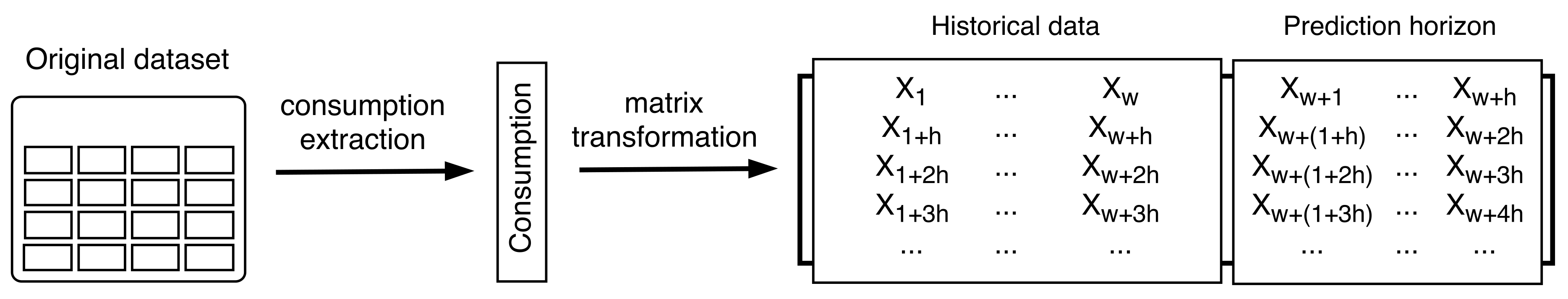
The original dataset has been pre-processed in order to be used, as in [35]. First, the attribute corresponding to consumption has been extracted, and a consumption vector has been obtained. After that, the consumption vector has been redistributed in a matrix depending on a historical window, w, and a prediction horizon, h. The historical window, or data history (w) represents the number of previous entries taken into consideration in order to train a model that will be used to predict the subsequent values (h). This process is detailed in Figure 2.
In this study, the prediction horizon (h) has been set to 24, corresponding to a period of 4 h. Moreover, different values of the data history have been used. In particular, w has been set to the values 24, 48, 72, 96, 120, 144 and 168, corresponding to 4, 8, 12, 16, 20, 24 and 28 h, respectively. The resulting datasets have been divided into for the training set and for the test set. Table 1 provides the details of each dataset. Notice that for all the obtained datasets, the last 24 columns represent the values to be predicted, and thus are not considered for training purposes.
3.2. Ensemble Learning
In the last few years, ensemble models are taking more relevance due to the good performance obtained in several tasks like classification or regression problems [44]. These methods consist in combining different learning models in order to improve the results obtained by each individual model.
The earliest works on ensemble learning were carried out in 1990s, e.g., [45,46,47], where it was proven that multiple weak learning algorithms could be converted into a strong learning algorithm. In a nutshell, ensemble learning [48,49] is a procedure where multiple learner modules are applied on a data set to extract multiple predictions. Such predictions are then combined into one composite prediction.
Usually two phases are employed. In a first phase a set of base learners are obtained from training data, while in the second phase the learners obtained in the first phase are combined in order to produce a unified prediction model. Thus, multiple forecasts based on the different base learners are constructed and combined into an enhanced composite model superior to the base individual models. This integration of all good individual models into one improved composite model generally leads to higher accuracy levels.
According to [48] there are three main reasons why ensemble learning is successful in ML. The first reason is statistical. Models can be seen as searching a hypothesis space H to identify the best hypothesis. However, since usually the datasets are limited, we can find many different hypotheses in H which can fit reasonably well, and we cannot establish a priori which one will generalize better, i.e., will perform the best on unseen data. This makes it difficult to choose among the hypotheses. It follows that the use of ensemble methods can help to avoid this issue by using several models to get a good approximation of the unknown true hypothesis.
The second reason is computational. Many models work by performing some form of local search to minimize error functions. These searches can get stuck in local optima. An ensemble constructed by starting the local search from many different points may provide a better approximation to the true unknown function.
The third argument is representational. In many situations, the unknown function we are looking for may not be included in H. However, a combination of several hypotheses drawn from H can enlarge the space of representable functions, which could then also include the unknown true function.
The most used and well-known of the basic ensemble methods are bagging, boosting and stacking.
- Bagging in this scheme, a number of models are built, the results obtained by these models are considered equally, and a voting mechanism is used in order to settle on the majority result. In case of regression the average predictions is usually the final output.
- Boosting is similar to bagging, but with one conceptual modification. Instead of assigning equal weighting to models, boosting assigns different weights to classifiers, and derives its ultimate result based on weighted voting. In case of regression a weighted average is usually the final output.
- Stacking builds its models using different learning algorithms and then a combiner algorithm is trained to make the ultimate predictions using the predictions generated by the base algorithms. This combiner can be any ensemble technique.
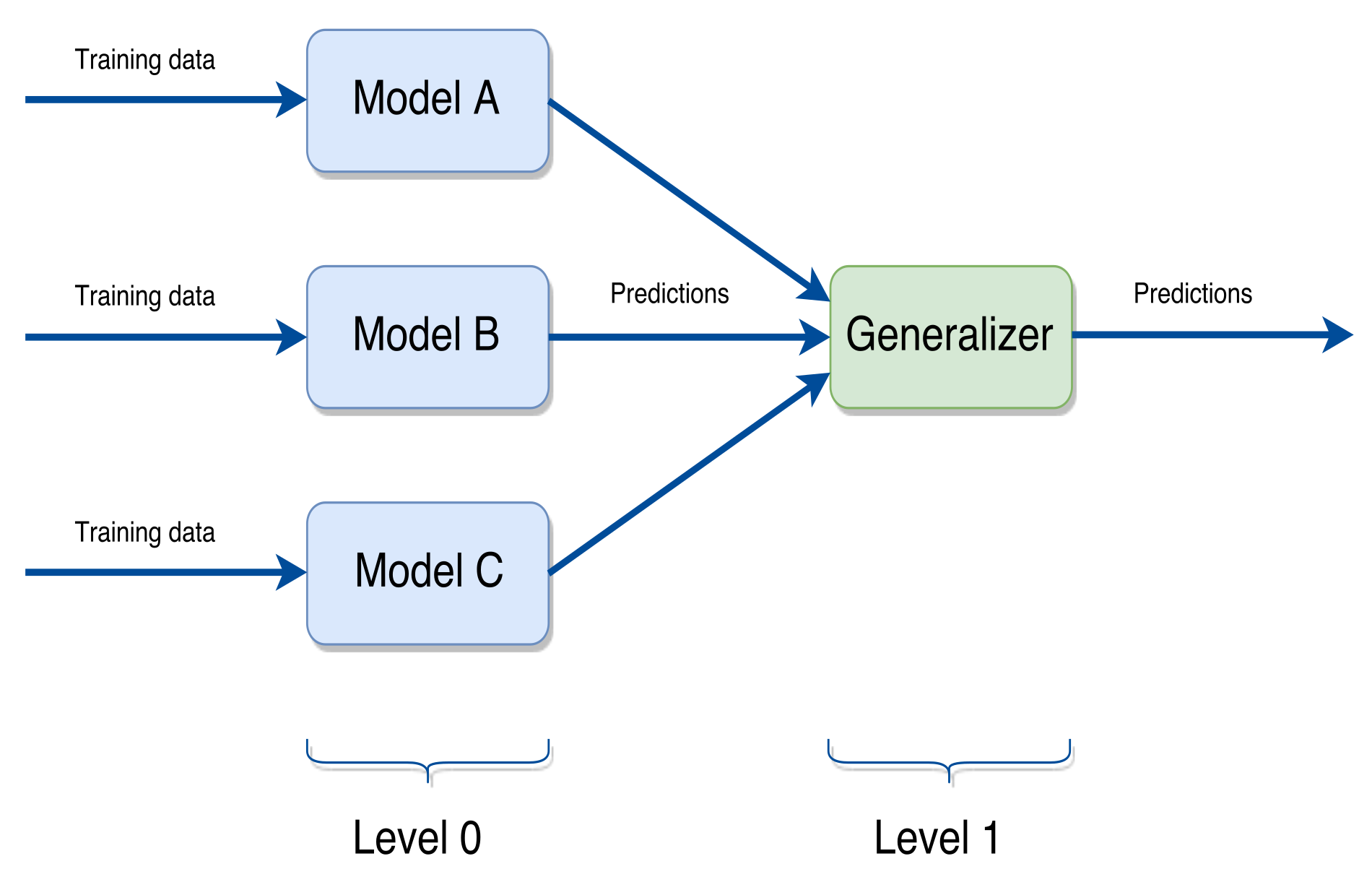
In this paper we have used a stacking approach, since we believe it to be the most suitable in case of the regression problem considered in this work. Figure 3 shows a general scheme of such approach. In the following section we will specify which learning algorithms have been used in the scheme we propose. We can define a stacking ensemble scheme more formally in the following way. Given a set of N different learning algorithms and the pair , with representing the w recorded values and the h values to predict. Let be the model induced by the learning algorithm on to predict , and let be the generalizer function responsible for combining the models for predicting such value. can be a generic function, such as the average, or a model induced by a learning algorithm. Then, the estimated value is given by the expression:
Ensemble methods have been successfully applied for solving pattern classification, regression and forecasting in time series problems [50,51]. For example, Adhikari [52] proposed a linear combination method for time series forecasting that determines the combining weights through a novel neural network structure. Bagnal et al. [53] proposed a method using an ensemble of classifiers on different data transformations in order to improve the accuracy of time-series classification. Authors demonstrated that the simple combination of all classifiers in one ensemble obtained better performance than any of its components. Jin and Dong [51] proposed a deep neural network-based ensemble method that integrates filtering views, local views, distorted views, explicit and implicit training, subview prediction, and Simple Average for classification of biomedical data. In particular, they used the Chinese Cardiovascular Disease cardiograms database. Chatterjee et al. [54] developed an ensemble support vector machine algorithm for reliability forecasting of a mining machine. This method is based on least square support vector machine (LS-SVM) with hyper parameters optimized by a Genetic Algorithm (GA). The output of this model was generalized from a combination of multiple SVM predicted results in time series dataset. Additionally, the advantages of ensemble methods for regression from different viewpoints such as strength-correlation or biasvariance was also demonstrate in the literature [55].
Ensemble learning based methods have been also applied in energy time series forecasting context. For example, Zang et al. [56] proposed a method, called extreme learning machine (ELM), which was successfully applied on the Australian National Electricity Market data. Another example was presented by Tan et al. in [57] where the authors proposed a price forecasting method based on wavelet transform combined with ARIMA and GARCH models. The method was applied on Spanish and PJM electricity markets. Fan et al. [58] proposed a ensemble machine learning model based on Bayesian Clustering by Dynamics (BCD) and SVM. The proposed model was trained and tested on the data of the historical load from New York City in order to forecasts the hourly electricity consumption. Tasnim et al. [59] proposed a cluster-based ensemble framework to predict wind power by using an ensemble of regression models on natural clusters within wind data. The method was tested on a large number of wind datasets of locations across spread Australia.
Ensembles of ANNs have been recently applied in the literature with the aim of energy consumption or price forecasting. For instance, the authors in [60] presented a building-level neural network-based ensemble model for day-ahead electricity load forecasting. The method showed that it outperforms the previously established best performing model by up to 50%, in the context of load data from operational commercial and industrial sites. Jovanovic et al. [61] used three artificial neural networks for prediction of heating energy consumption of a university campus. The authors tested the neural networks with different parameter combinations, which, when used in an ensemble scheme, achieved better results.
3.3. Methods
As already stated in Section 3.2, in our proposal we used a stacking ensemble scheme. In particular, we employed a scheme formed by three base learning methods and a top method. The basic learning methods are regression trees based on Evolutionary Algorithms, Artificial Neural Networks and Random Forests. At the top level, we have used the Generalized Boosted Regression Models in order to combine the predictions produced by the bottom level. The employed scheme is graphically shown in Figure 4.
In the following, we provide some basic notions regarding the methods used in the ensemble scheme.
- Evolutionary Algorithms (EAs) for Regression Trees EAs [62] are population-based strategies that use techniques inspired by evolutionary biology such as inheritance, mutation, selection and crossover. Each individual i of the population represents a candidate solution to a given problem and is assigned a fitness function, which is a measure of the quality of the solution represented by i. Typically EAs start from an initial population consisting of randomly initialised individuals. Each individual is evaluated in order to determine its fitness value. Then a selection mechanism is used in order to select a number of individuals. Usually the selection is based on the fitness, so that fitter individuals have more probabilities of being selected. Selected individuals generate offspring, i.e., new solutions, by means of the application of crossover and mutation operators. This process is repeated over a number of generations or until a good enough solution is found. The idea is that better and better solutions will be found at each generation. Moreover, the use of stochastic operators, such as mutation, allows EAs to escape from local optima. For the problem tackled in this paper, each individual encodes a regression tree. A regression tree is a decision tree similar to a classification tree [63]. Both classification and regression trees aim at modeling a response variable Y by a vector of P predictor variables . The different is that for classification trees, Y is qualitative and for regression trees Y is quantitative. In both cases can be continuous and/or categorical variables.Regression trees are commonly used in regression-type problems, where we attempt to predict the values of a continuous variable from one or more continuous and/or categorical predictor variables. An advantage of using regression trees is that results can be easier to interpret. Other greedy strategies have been used in order to obtained regression trees, for example [64,65]. The main challenge of such strategiesis that the search space is typically huge, rendering full-grid searches computationally infeasible. Due to their search capabilities, EAs have proven that they can overcome this limitation.In this paper, we have used the R evtree package (from now on EVTree) [66], with the following parameters:
- minbucket: 8 (minimum number of observations in each terminal node)
- minsplit: 100 (minimum number of observations in each internal node)
- maxdepth: 15 (maximum tree depth)
- ntrees: 300 (number of tree in the population)
- niterations: 1000 (maximum number of generations)
- alpha: 0.25 (complexity part of the cost function)
- operatorprob: with this parameter, we can specify, in list or vector form, the probabilities for the following variation operators:
- –
- pmutatemajor: 0.2 (Major split rule mutation, selects a random internal node r and changes the split rule, defined by the corresponding split variable , and the split point [66])
- –
- pmutateminor: 0.2 (Minor split rule mutation is similar to the major split rule mutation operator. However, it does not alter and only changes the split point by a minor degree, which is defined by four cases describes in [66])
- –
- pcrossover: 0.8 (Crossover probability)
- –
- psplit: 0.2 (Split selects a random terminal-node and assigns a valid, randomly generated, split rule to it. As a consequence, the selected terminal node becomes an internal node r and two new terminal nodes are generated)
- –
- pprune: 0.4 (Prune chooses a random internal node r, where r > 1, which has two terminal nodes as successors and prunes it into a terminal node [66])
- Artificial Neural Networks (ANNs) ANNs [67] are computational models inspired by the structure and functions of biological neural networks. The basic unit of computation is the neuron, also called node, which receives input from other nodes or from an external source and computes an output. In order to compute such output, the node applies a function f called the Activation Function, which has the purpose of introducing non-linearity into the output. Furthermore, the output is produced only if the inputs are above a certain threshold.Basically, an ANN creates a relationship between input and output values and is composed of interconnected nodes grouped in several layers. Among such layers we can distinguish the outer ones, called input and output layers, from the “internal” ones, called hidden layers. In contrast to biological neurons networks, ANNs usually consider only one type of node, in order to simplify the model calculation and analysis.The intensity of the connection between nodes is determined by weights, which are modified during the learning process. Therefore, the learning process consists in adapting the connections to the data structure that model the environment and to characterize its relations.According to the structure, there are different types of ANN. The suitability of the structure depends on several factors as, for example, the quality and the volume of the input data. The simplest type of ANN is the so called feedforward neural network. In such networks, nodes from adjacent layers are interconnected and each connection has a weight associated to it. The information moves forward from the input to the output layer through the hidden nodes. There is only one node at the output layers, which provides the final results of the network, being it a class label or a numeric value.In this paper we have used the nnet package of R [68], a package for feed-forward neural networks with a single hidden layer, and for multinomial log-linear models.The following parameters were used in this paper:
- size: 10 (number of hidden units)
- skip: true (add skip-layer connections from input to output)
- MaxNWts: 10,000 (maximum number of weights allowed)
- maxit: 1000 (maximum number of iterations)
- Random Forests (RF) The term Random Forest was introduced by Breinman and Cutle in [69], and refers to a set of decision trees which form an ensemble of predictors. Thus, RF is basically an ensemble of decision trees, where each tree is trained separately on a idependent randomly selected training set. It follows that each tree depends on the values of an input dataset sampled independently, with the same distribution for all trees.In other words, the trees generated are different since they are obtained from different training sets from a bootstrap subsampling and different random subsets of features to split on at each tree node. Each tree is fully grown, in order to obtain low-bias trees. Moreover, at the same time, the random subsets of features result in low correlation between the individual trees, so the algorithm yields an ensemble that can achieve both, low bias and low variance [70]. For classification, each tree in the RF casts a unit vote for the most popular class at input. The final result of the classifier is determined by a majority vote of the trees. For regression, the final prediction is the average of the predictions from the set of decision trees.The method is less computationally expensive than others tree-based classifiers that adopt bagging strategies, since each tree is generated by taking into account only a portion of the input features [71].In this paper, we have used the implementation from the randomForest package of R [72], which provides a R interface to the original implementation by Breiman and Cutle. For this study, the algorithm is used with the following parameters:
- ntree : 100 (number of trees to be built by algorithm).
- maxnodes: 100 (maximum number of terminal nodes trees in the forest can have).
- Generalized Boosted Regression Models (GBM) [73,74]. This method iteratively trains a set of decision trees. The current ensemble of trees is used in order to predict the value of each training example. The prediction errors are then estimated, and poor predictions are adjusted, so that in the next iterations the previous mistakes are corrected. Gradient boosting involves three elements:
- A loss function to be optimised. Such function is problem dependent. For instance, for regression a squared error can be used and for classification we could use logarithmic loss.
- A weak learner to make predictions. Regression trees are used to this aim, and a greedy strategy is used in order to build such trees. This strategy is based on using a scoring function used each time a split point has to be added to the tree. Other strategies are commonly adopted in order to constrain the trees. For examples one may limit the depth of the tree, the number of splits or the number of nodes.
- An additive model to add trees to minimise the loss function. This is done in a sequential way, and the trees already contained in the model built so far are not changed. In order to minimise the loss during this phase, a gradient descend procedure is used. The procedure stops when a maximum number of trees has been added to the model or once there is no improvement in the model.
Overfitting is common in gradient boosting, and usually, some regularisation methods are used in order to reduce it. These methods basically penalise various parts of the algorithm. Usually some mechanisms are used in order to impose constraints on the construction of decision trees, for example limit the depth of the trees, the number of nodes or leafs or the number of observation per split.Another mechanism is shrinkage, which is basically weighting the contribution of each tree to the sequential sum of the predictions of the trees. This is done with the aim of slowing down the learning rate of the algorithm. As a consequence the training takes longer, since more trees are added to the model. In this way a trade-off between the learning rate and the number of trees can be reached.In this paper we have used the GBM package of R [75] with the following parameters:- distribution: Gaussian (function of the distribution to use)
- n.trees: 3000 (total number of trees, i.e., the number of gradient boosting iteration)
- interaction.depth: 40 (maximum depth of variable interactions)
- shrinkage: 0.9 (learning rate)
- n.minobsinnode: 3 (minimum number of observations in the trees terminal nodes)
All the parameters used in this paper were set after running preliminary experiments on the data.
We have selected the strategies forming our ensemble scheme based on their popularity and good results achieved in similar problems. Moreover, we have selected algorithms that base the predictions on decision trees, and complemented the possible weakness of such methods by using Artificial Neural Networks. In particular, both RF and GBM are based on an ensemble of decision trees, but the set of trees is obtained in a different way, with RF building each tree independently. EAs provide the ability of escaping local optima, thus we believe that these methods complement each other. Moreover, in order to overcome possible representation limitations of decision trees, we have used NNs, which can handle very well non-linear learning and are tolerant to noise. GBM training generally takes longer than RF, since trees are built sequentially. Moreover, decision trees obtained are prone to overfitting, so we have used it on the top layer, where the predictions are based on three columns, i.e., the output of the three base learners.
The final ensemble scheme we proposed is depicted in Figure 5. We can see that the training set is used in order to obtain the predictions of the base level, consisting of RF, NN and EVTree. The so obtained predictions are then used by the top layer (GBM) in order to produce the final predictions for each problem.
Then, according to the notation introduced in Section 3.2, EVTree, ANN and = RF, , and are the models induced by EVTree, ANN and RF, respectively, while is the model produced by GBM. Thus the final predictions are produced by GBM, which builds the model using the predictions generated by the three bottom layer methods.
4. Results
In this section we provide the results obtained on the dataset described in Section 3.1 and draw the main conclusions. In order to assess the performances of both the ensemble scheme and the base methods, we used five measures commonly used in regression: the mean relative error (MRE), the mean absolute error (MAE), the symmetric mean absolute percentage error (SMAPE), the coefficient of determination , and the root mean squared error (RMSE), which are defined as [16]:
In the above equations, is the predicted value, the real value and is the mean of the observed data.
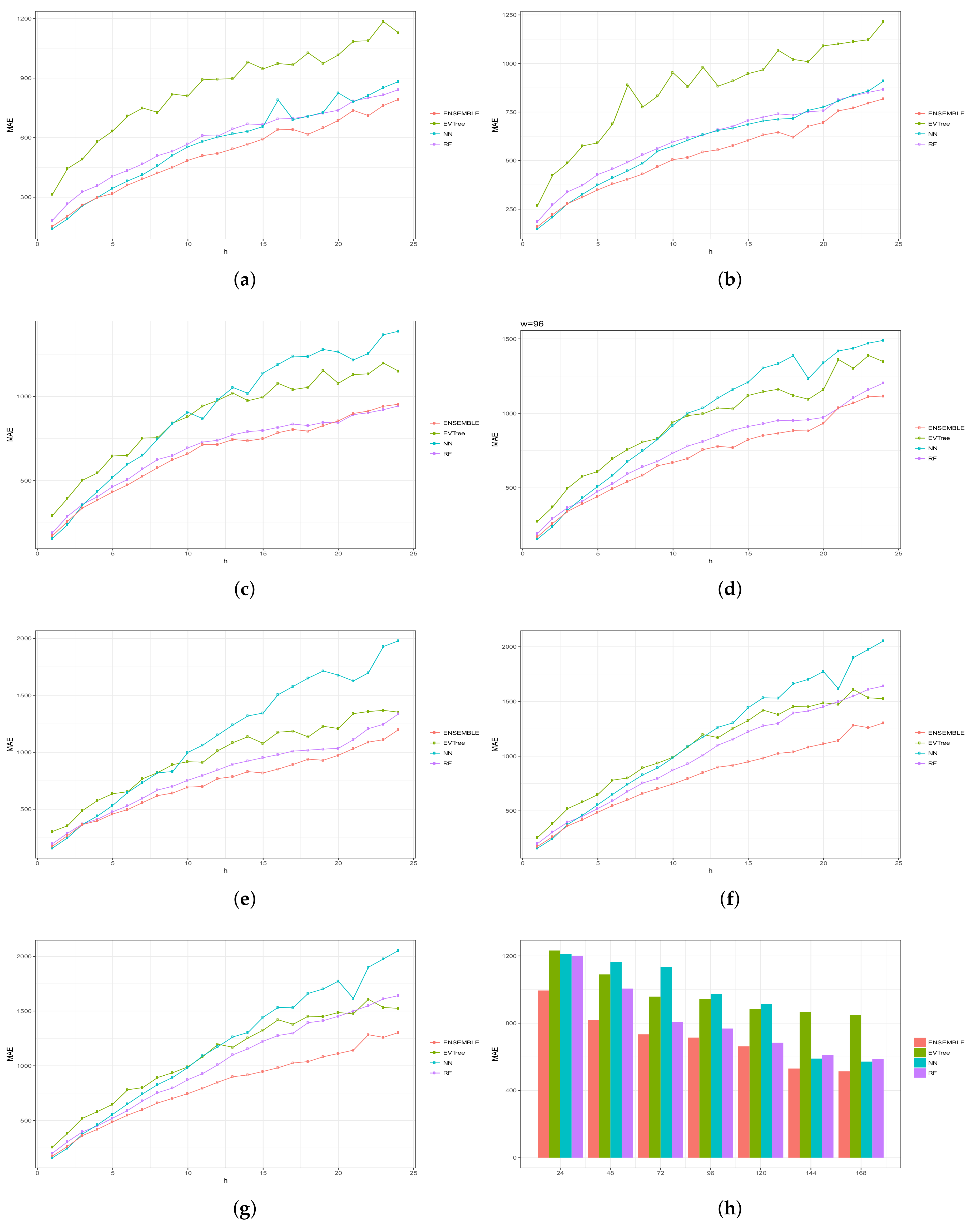
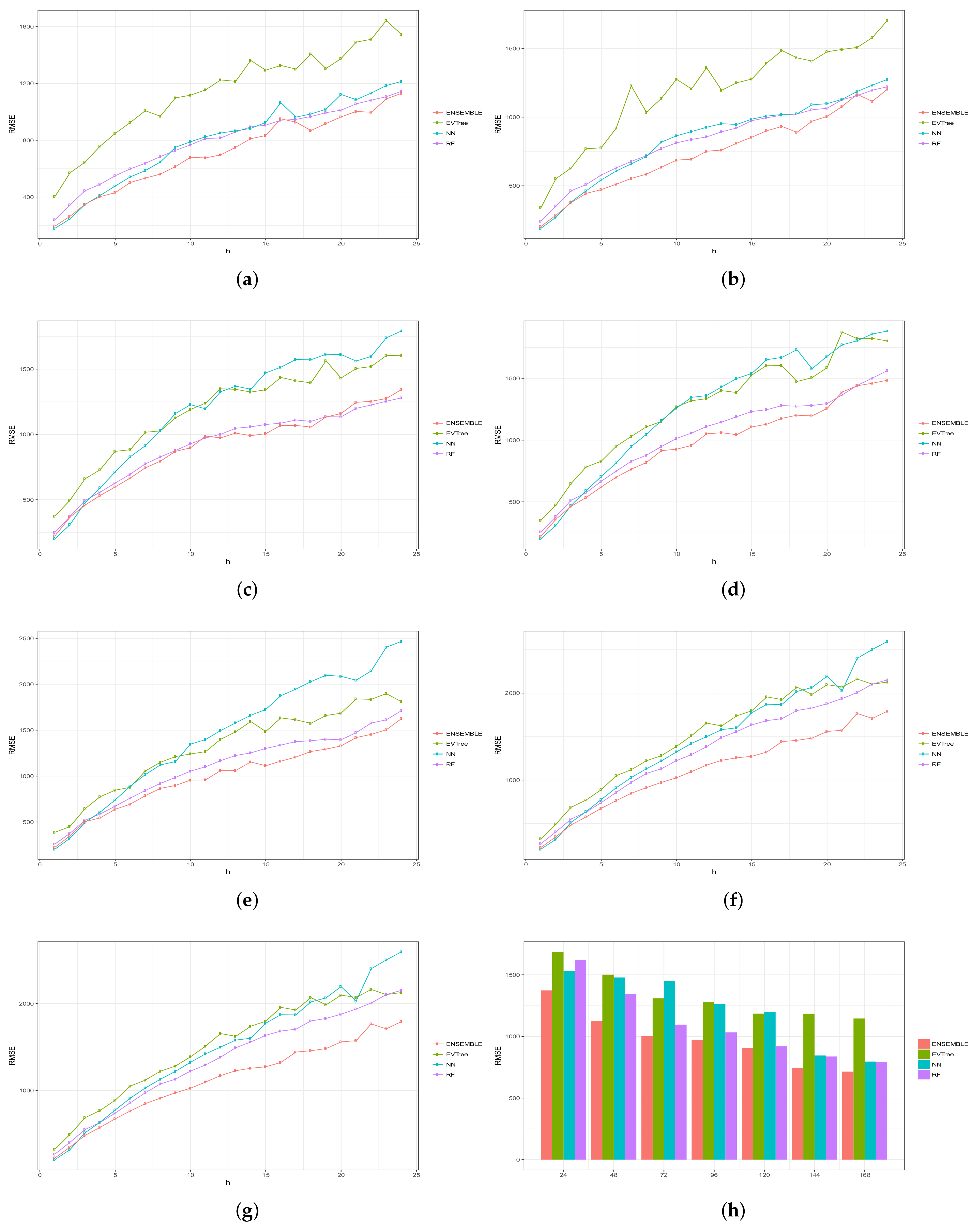
Figure 6, Figure 7, Figure 8, Figure 9 and Figure 10 show the results obtained on all the problems (h) for each historical window (w) used by both the algorithms employed in the bottom layer (EVTree, NN and RF) and by the top layer of the ensemble scheme (GBM). The average results obtained are also shown in the bar graphs. The detailed results obtained by the ensemble scheme and by the base methods can be found in Appendix A, and in particular in Table A1, Table A2, Table A3, Table A4 and Table A5, where results are grouped by the size of the historical window used, as indicated by the first row.
The first and main conclusion that we can draw from these graphs is that the best results were obtained when all the predictions of the baseline methods were combined by GBM at the top level of the ensemble scheme. In particular, when using a historical window of 168 measuraments, the average MRE obtained was , while the was , the MAE was , the RMSE and the average sMAPE was . In order to assess the significance of the results with respect to the results obtained, we applied a statistical paired two-tailed t-test with confidence level of . According to this test, all the results are significantly different, a part from the MRE, MAE, RMSE and sMAPE obtained by EVTree and NN when historical windows of and 48 were used. Moreover, when w was set to 24, all the results obtained by the bottom layer methods were not significantly different, as far as MRE, MAE and sMAPE are concerned. When we consider MAE, RMSE and sMAPE, results obtained by RF and NN are considered equal for a historical window of 168. The same holds when is considered, moreover, in the case of , results obtained by these two methods are not considered significantly different for a historical window of 120 as well. Considering again , results obtained by EVTree and NN are considered equal for historical windows of size 120 and 72. The results produced by the top layer were always significantly better in all the cases but when considering for a historical window equal to 120. In this case results obteind by RF are not significantly different. Results obtained by RF and NN are not considered different for historical window values of 144 and 120 as far as RMSE is concerned.
Results are summarized in Table 2, where a ranking of the methods is shown, according to the MRE obtained.
In general, we can also notice the degradation of performances of NN when the historical window used is reduced. In fact, for a historical window of 168, NN obtains the best results among the three bottom layer methods, while for smaller historical windows, starting from 120 measurements, the predictions obtained by this method are always worst than those obtained by RF, and are comparable or worst than the predictions produced by EVTree. Similar consideration can be extracted for the other measures.
We can also notice that the predictions are less and less accurate for increasing values of p, meaning that it is easier to predict the very near future demand than the medium-far future demand. In this sense, we can also observe that NN performs really well on the first two problems. In fact, for values of p equals to 1 or 2, in many cases the predictions obtained by NN are superior to those obtained by the top layer. However, as the value of p increments, the results obtained by the top layer are much better than the results achieved by the three bottom methods. Basically the real difference is made when the problems become harder and harder.
Finally, in Figure 11, we present a comparison of the real and predicted values for a subset of the time series when a historical window of 168 was used. For readability reasons, we have selected two subsets of 250 and 1000 readings, respectively shown in Figure 11a,b. We have included the figure regarding 250 in order to provide a more detailed view of the predictions. We can notice that the predictions are very accurate, and that they can describe in a very precise way the original time series.
In order to globally assess the performance of our proposal, we have compared the results achieved by our ensemble scheme with the results obtained by the single components used in our proposal, i.e., Random Forest (RF), Neural Networks (NN) and Evolutionary Decition Trees (EV), and the results obtained by other four state of the art methods: linear regression (LR), ARMA and ARIMA, Deep Learning (DL) and a decision tree algorithm (DT). In particular we have taken into account linear regression, as a reference time series forecasting strategy [76,77]. The well-known stochastic gradient descent method has been used to minimise the mean square error for the training set in order to obtain the model. We have used a decision tree greedy algorithm [78] that performs a recursive binary partitioning of the feature space in order to build a decision tree. This algorithm uses the information gain in order to build the decision trees, and we have used the default parameter as in the package rpart of R [79]. For the conventional methods ARMA and ARIMA, we have used a tool [80] for determining the order of auto-regressive (AR) terms (p), the degree of differencing (d) and the order of moving-average (MA) terms (q). The values obtained are , and . The deep learning-based methodology has been designed using framework of R [81]. This framework implements a Feed Forward Neural Network (also called multi-layer perceptron) that can be launched in distributed environments. The network is trained with stochastic gradient descend using back-propagation algorithm. In order to set the parameters for this algorithm, we have used a grid search approach. As a consequence, we have used a hyperbolic tangent function as activation function, the number of hidden layer was set to 3 and the number of neurons to 30. The distribution function was set to Poisson and in order to avoid overfitting, one of two regularization parameter (Lambda) has ben set to 0.001. The other parameter were set as default as in [35].
Table 3 shows the results of such comparison for each value of historical window considered. We can notice that our proposal outperforms all the other methods, obtaining the best results in all the historical window values considered. This is particularly noticeable for smaller values of w. Another conclusion that we can draw from the table is that LR and NN obtains good results, which are comparable, especially on higher values of the historical window w. Among the single methods, RF obtains, in general, good results, especially for smaller values of historical. It can be noticed that RF achieves better results than LR and NN strategies in all cases except for w values 144 and 168, while it outperforms DL and EV in all cases. In general, the classical strategies ARMA and ARIMA do not perform well on this problem. DT does not perform well on this problem either. This is probably due to the greedy strategy used by this algorithm, which may cause it to get stuck in some local optima. The same considerations may be done for GBM, even if the ensemble nature of this algorithm provides an advantage over DT, and so the results obtained are better. In general we can conclude that the results obtained on this problem by the ensemble scheme are satisfactory, as they achieve more accurate predictions for this short-term electricity consumption forecast problem.
5. Conclusions and Future Works
Accurate short-term forecasting regarding the electric energy demand would provide several benefits, both economical and environmental. For instance, predictions can be taken into account in order to reduce the costs of energy productions, decreasing in the same way the impact on the environment. The predictions are made by taking into consideration data regarding the past demand of electricity, i.e., taking into account historical data. In short-term forecasting, the aim is to be able to predict the near future demand.
In this paper, we have approached the electric energy short-term forecasting problem with a methodology based on ensemble learning. Ensemble learning allows to combine the predictions made by different learning mechanisms in order to achieve predictions that are usually more accurate. More specifically, we have used a stacking ensemble learning scheme, where two levels of learning methods are used. The prediction made by the first level methods are passed to a top method which combines them in order to produce the final forecastings. In this paper, we have used three base learning methods, i.e, regression trees based on Evolutionary Computation, Random Forest and Artificial Neural Networks. At the top layer we have used an algorithm based on Gradient Boosting. We have considered different historical windows, i.e., different amount of historical data used in order to obtain a prediction, and we have focused on predicting the electricity demand of the following four hours. We have compared the results obtained by the ensemble method with the results obtained by the single methods and by linear regression and a decision tree algorithm. Predictions obtained by the ensemble scheme were always superior to the result of the other methods. We have also observed that some methods, like NN, are able to make very precise predictions in the very near future, but that results degenerates the further in the future we aim to predict. Moreover, when the size of historical windows used is small, results are significantly improved when the ensemble scheme is employed. This is due to the degradation in performances of single methods that need the support of more historical data in order to achieve acceptable results.
As for future works, we intend to explore other ensemble schemes, using different methods, for example methods based on support vector machines, deep learning [82] or methods based on SP Theory of Intelligence [83]. Moreover, we are planning on using other datasets, both regarding the electric energy consumption, but also other kind of time series, in order to check if our approach can be generalized to other kind of problems.
Acknowledgments
This work was supported by the Spanish Ministry of Economic and Competitiveness and the European Regional Development Fund, under the grant TIN2015-64776-C3-2-R (MINECO/FEDER). Authors are also thankful to the Andalusian Scientific Computer Science Centre (CICA) for allowing us to use their computing infrastructures.
Author Contributions
Federico Divina proposed the concept of this research and has been involved in the whole experimentation phase. Aude Gilson has carried out the analysis using the evolutionary algorithm and contributed to the building and experimentation of the ensemble learning scheme. Francisco A. Goméz Vela has been involved in the experimentation, while José F. Torres has preprocessed the datasets. Miguel García Torres has provided overall guidance and has been involved in the experimentation. All the authors were involved in preparing the manuscript.
Conflicts of Interest
The authors declare no conflict of interest.
Appendix A. Detailed Results of the Ensemble Scheme

Table A1.
MRE obtained for each historical window considered and each problem. In the table EV stands for EVTree, RF for Random Forest, NN for Neural Network. GBM stand for the Gradient Boost Models, the method used at the top level, and thus represent the final MRE obtained by the ensemble method.
Table A1.
MRE obtained for each historical window considered and each problem. In the table EV stands for EVTree, RF for Random Forest, NN for Neural Network. GBM stand for the Gradient Boost Models, the method used at the top level, and thus represent the final MRE obtained by the ensemble method.
| w | 168 | 144 | 120 | 96 | 72 | 48 | 24 | ||||||||||||||||||||||
|---|---|---|---|---|---|---|---|---|---|---|---|---|---|---|---|---|---|---|---|---|---|---|---|---|---|---|---|---|---|
| h | EV | RF | NN | GBM | EV | RF | NN | GBM | EV | RF | NN | GBM | EV | RF | NN | GBM | EV | RF | NN | GBM | EV | RF | NN | GBM | EV | RF | NN | GBM | |
| 1 | 1.15 | 0.66 | 0.53 | 0.57 | 0.98 | 0.67 | 0.55 | 0.59 | 1.08 | 0.58 | 0.57 | 0.64 | 1.01 | 0.70 | 0.57 | 0.63 | 1.11 | 0.69 | 0.59 | 0.64 | 0.93 | 0.73 | 0.59 | 0.64 | 0.94 | 0.74 | 0.59 | 0.64 | |
| 2 | 1.63 | 0.96 | 0.98 | 0.75 | 1.58 | 0.98 | 0.78 | 0.82 | 1.44 | 1.03 | 0.88 | 0.93 | 1.36 | 1.05 | 0.88 | 0.95 | 1.30 | 1.06 | 0.89 | 0.97 | 1.39 | 1.09 | 0.91 | 0.96 | 1.43 | 1.15 | 0.92 | 1.00 | |
| 3 | 1.81 | 1.18 | 1.10 | 0.95 | 1.75 | 1.21 | 1.01 | 1.01 | 1.83 | 1.27 | 1.28 | 1.21 | 1.79 | 1.34 | 1.27 | 1.23 | 1.77 | 1.32 | 1.33 | 1.31 | 1.86 | 1.42 | 1.34 | 1.31 | 1.79 | 1.53 | 1.35 | 1.37 | |
| 4 | 2.10 | 1.28 | 1.14 | 1.09 | 2.09 | 1.33 | 1.19 | 1.13 | 1.97 | 1.43 | 1.54 | 1.38 | 2.08 | 1.45 | 1.56 | 1.41 | 2.10 | 1.48 | 1.63 | 1.43 | 2.10 | 1.60 | 1.64 | 1.50 | 2.09 | 1.79 | 1.66 | 1.65 | |
| 5 | 2.31 | 1.46 | 1.26 | 1.16 | 2.11 | 1.53 | 1.38 | 1.27 | 2.30 | 1.65 | 1.87 | 1.54 | 2.22 | 1.70 | 1.85 | 1.58 | 2.29 | 1.72 | 1.98 | 1.63 | 2.34 | 1.86 | 1.98 | 1.73 | 2.58 | 2.11 | 2.00 | 1.85 | |
| 6 | 2.57 | 1.54 | 1.40 | 1.32 | 2.46 | 1.63 | 1.51 | 1.38 | 2.34 | 1.80 | 2.15 | 1.69 | 2.53 | 1.86 | 2.13 | 1.76 | 2.37 | 1.90 | 2.30 | 1.78 | 2.79 | 2.11 | 2.29 | 1.95 | 2.76 | 2.42 | 2.34 | 2.14 | |
| 7 | 2.71 | 1.69 | 1.55 | 1.43 | 3.23 | 1.76 | 1.64 | 1.47 | 2.70 | 2.02 | 2.34 | 1.87 | 2.73 | 2.11 | 2.42 | 1.94 | 2.77 | 2.14 | 2.51 | 1.99 | 2.87 | 2.40 | 2.64 | 2.15 | 3.17 | 2.76 | 2.66 | 2.38 | |
| 8 | 2.63 | 1.83 | 1.67 | 1.54 | 2.80 | 1.91 | 1.80 | 1.56 | 2.73 | 2.21 | 2.65 | 2.06 | 2.92 | 2.35 | 2.70 | 2.10 | 2.99 | 2.38 | 2.79 | 2.22 | 3.23 | 2.68 | 2.94 | 2.37 | 3.49 | 3.11 | 2.97 | 2.76 | |
| 9 | 2.90 | 1.91 | 1.84 | 1.63 | 2.99 | 2.00 | 1.99 | 1.69 | 2.98 | 2.28 | 2.96 | 2.21 | 2.99 | 2.43 | 3.00 | 2.30 | 3.20 | 2.50 | 3.23 | 2.29 | 3.37 | 2.82 | 3.19 | 2.50 | 3.90 | 3.34 | 3.36 | 2.89 | |
| 10 | 2.92 | 2.07 | 2.01 | 1.75 | 3.45 | 2.13 | 2.12 | 1.81 | 3.15 | 2.43 | 3.21 | 2.33 | 3.33 | 2.66 | 3.32 | 2.37 | 3.30 | 2.70 | 3.52 | 2.46 | 3.58 | 3.05 | 3.58 | 2.66 | 3.75 | 3.71 | 3.68 | 3.07 | |
| 11 | 3.23 | 2.21 | 2.10 | 1.86 | 3.21 | 2.23 | 2.21 | 1.88 | 3.40 | 2.58 | 3.43 | 2.53 | 3.57 | 2.81 | 3.56 | 2.48 | 3.27 | 2.85 | 3.77 | 2.49 | 3.86 | 3.36 | 3.85 | 2.83 | 4.15 | 4.00 | 4.02 | 3.30 | |
| 12 | 3.24 | 2.24 | 2.20 | 1.90 | 3.58 | 2.28 | 2.28 | 1.96 | 3.47 | 2.63 | 3.45 | 2.53 | 3.62 | 2.92 | 3.72 | 2.70 | 3.66 | 2.99 | 4.14 | 2.74 | 4.30 | 3.70 | 4.10 | 3.04 | 4.55 | 4.33 | 4.33 | 3.56 | |
| 13 | 3.26 | 2.36 | 2.25 | 1.98 | 3.21 | 2.39 | 2.36 | 2.02 | 3.71 | 2.75 | 3.69 | 2.63 | 3.72 | 3.07 | 3.77 | 2.79 | 3.90 | 3.20 | 4.44 | 2.82 | 4.19 | 3.92 | 4.54 | 3.22 | 4.79 | 4.69 | 4.71 | 3.84 | |
| 14 | 3.58 | 2.50 | 2.30 | 2.08 | 3.29 | 2.48 | 2.42 | 2.10 | 3.50 | 2.81 | 3.86 | 2.63 | 3.75 | 3.20 | 4.19 | 2.75 | 4.12 | 3.37 | 4.56 | 3.00 | 4.59 | 4.21 | 4.92 | 3.29 | 4.99 | 4.95 | 5.04 | 3.90 | |
| 15 | 3.45 | 2.43 | 2.37 | 2.16 | 3.41 | 2.56 | 2.48 | 2.21 | 3.59 | 2.83 | 4.09 | 2.66 | 4.05 | 3.24 | 4.43 | 2.93 | 3.91 | 3.41 | 5.09 | 2.93 | 4.79 | 4.42 | 5.19 | 3.38 | 5.63 | 5.19 | 5.42 | 4.29 | |
| 16 | 3.54 | 2.53 | 2.47 | 2.37 | 3.51 | 2.62 | 2.57 | 2.30 | 3.88 | 2.91 | 4.23 | 2.80 | 4.24 | 3.34 | 4.57 | 3.06 | 4.25 | 3.51 | 5.16 | 3.05 | 5.21 | 4.65 | 5.35 | 3.53 | 5.40 | 5.46 | 5.76 | 4.24 | |
| 17 | 3.52 | 2.58 | 2.48 | 2.36 | 3.89 | 2.70 | 2.58 | 2.36 | 3.77 | 2.98 | 4.40 | 2.88 | 4.24 | 3.40 | 4.90 | 3.12 | 4.24 | 3.61 | 5.73 | 3.20 | 5.07 | 4.86 | 5.87 | 3.70 | 5.74 | 5.82 | 6.09 | 4.51 | |
| 18 | 3.75 | 2.61 | 2.55 | 2.27 | 3.70 | 2.69 | 2.65 | 2.28 | 3.78 | 2.99 | 4.48 | 2.86 | 4.02 | 3.42 | 4.84 | 3.18 | 4.12 | 3.67 | 5.93 | 3.37 | 5.37 | 5.11 | 6.14 | 3.77 | 6.03 | 6.00 | 6.45 | 4.75 | |
| 19 | 3.55 | 2.70 | 2.62 | 2.41 | 3.65 | 2.77 | 2.72 | 2.47 | 4.20 | 2.99 | 4.53 | 3.01 | 3.97 | 3.47 | 5.18 | 3.21 | 4.46 | 3.77 | 6.22 | 3.35 | 5.37 | 5.29 | 6.40 | 3.96 | 6.28 | 6.19 | 5.74 | 4.91 | |
| 20 | 3.75 | 2.78 | 2.78 | 2.55 | 3.99 | 2.81 | 2.87 | 2.56 | 3.95 | 3.12 | 4.66 | 3.12 | 4.24 | 3.57 | 5.19 | 3.38 | 4.50 | 3.87 | 6.49 | 3.54 | 5.55 | 5.38 | 6.54 | 4.08 | 6.14 | 6.45 | 6.89 | 5.17 | |
| 21 | 4.02 | 2.91 | 2.89 | 2.72 | 4.05 | 3.01 | 2.93 | 2.80 | 4.10 | 3.23 | 4.64 | 3.28 | 4.94 | 3.85 | 5.13 | 3.75 | 4.89 | 4.09 | 6.26 | 3.74 | 5.49 | 5.63 | 6.57 | 4.18 | 6.55 | 6.79 | 6.84 | 5.45 | |
| 22 | 4.02 | 2.95 | 3.01 | 2.63 | 4.06 | 3.09 | 3.08 | 2.85 | 4.14 | 3.34 | 4.76 | 3.32 | 4.79 | 4.12 | 5.26 | 3.88 | 4.93 | 4.39 | 6.55 | 3.95 | 5.98 | 6.03 | 7.14 | 4.72 | 6.85 | 7.16 | 7.16 | 5.63 | |
| 23 | 4.38 | 3.05 | 3.16 | 2.83 | 4.14 | 3.16 | 3.24 | 2.95 | 4.40 | 3.43 | 0.85 | 3.44 | 5.14 | 4.33 | 5.38 | 4.07 | 5.01 | 4.70 | 6.71 | 4.03 | 5.71 | 6.08 | 7.24 | 4.63 | 7.21 | 7.62 | 7.53 | 6.10 | |
| 24 | 4.13 | 3.08 | 3.30 | 2.93 | 4.46 | 3.21 | 3.36 | 3.04 | 4.21 | 3.48 | 5.03 | 3.48 | 4.89 | 4.43 | 5.39 | 4.09 | 4.98 | 5.00 | 7.37 | 4.37 | 5.68 | 6.30 | 7.59 | 4.78 | 7.52 | 7.97 | 7.86 | 6.60 | |
| avg | 3.09 | 2.15 | 2.08 | 1.88 | 3.15 | 2.22 | 2.16 | 1.94 | 3.19 | 2.45 | 3.15 | 2.38 | 3.42 | 2.78 | 3.55 | 2.57 | 3.48 | 2.93 | 4.13 | 2.64 | 3.98 | 3.70 | 4.27 | 2.95 | 4.49 | 4.39 | 4.39 | 3.58 | |
| stdev | 0.84 | 0.69 | 0.75 | 0.67 | 0.90 | 0.71 | 0.78 | 0.69 | 0.95 | 0.80 | 1.41 | 0.81 | 1.15 | 1.04 | 1.56 | 0.97 | 1.18 | 1.16 | 2.05 | 1.00 | 1.52 | 1.71 | 2.16 | 1.20 | 1.91 | 2.14 | 2.23 | 1.65 | |
Table A2.
obtained for each historical window considered and each problem. In the table EV stands for EVTree, RF for Random Forest, NN for Neural Network. GBM stand for the Gradient Boost Models, the method used at the top level, and thus represent the final obtained by the ensemble method.
Table A2.
obtained for each historical window considered and each problem. In the table EV stands for EVTree, RF for Random Forest, NN for Neural Network. GBM stand for the Gradient Boost Models, the method used at the top level, and thus represent the final obtained by the ensemble method.
| w | 168 | 144 | 120 | 96 | 72 | 48 | 24 | ||||||||||||||||||||||
|---|---|---|---|---|---|---|---|---|---|---|---|---|---|---|---|---|---|---|---|---|---|---|---|---|---|---|---|---|---|
| h | EV | RF | NN | GBM | EV | RF | NN | GBM | EV | RF | NN | GBM | EV | RF | NN | GBM | EV | RF | NN | GBM | EV | RF | NN | GBM | EV | RF | NN | GBM | |
| 1 | 0.99 | 1.00 | 1.00 | 1.00 | 0.99 | 1.00 | 1.00 | 1.00 | 0.99 | 1.00 | 1.00 | 1.00 | 0.99 | 1.00 | 1.00 | 1.00 | 0.99 | 1.00 | 1.00 | 1.00 | 0.99 | 1.00 | 1.00 | 1.00 | 0.99 | 1.00 | 1.00 | 1.00 | |
| 2 | 0.98 | 0.99 | 1.00 | 1.00 | 0.98 | 0.99 | 1.00 | 1.00 | 0.99 | 0.99 | 1.00 | 0.99 | 0.99 | 0.99 | 0.99 | 0.99 | 0.99 | 0.99 | 0.99 | 0.99 | 0.99 | 0.99 | 0.99 | 0.99 | 0.99 | 0.99 | 0.99 | 0.99 | |
| 3 | 0.98 | 0.99 | 0.99 | 0.99 | 0.98 | 0.99 | 0.99 | 0.99 | 0.98 | 0.99 | 0.99 | 0.99 | 0.98 | 0.99 | 0.99 | 0.99 | 0.98 | 0.99 | 0.99 | 0.99 | 0.98 | 0.98 | 0.99 | 0.99 | 0.98 | 0.98 | 0.99 | 0.98 | |
| 4 | 0.97 | 0.99 | 0.99 | 0.99 | 0.97 | 0.99 | 0.99 | 0.99 | 0.97 | 0.98 | 0.98 | 0.99 | 0.97 | 0.98 | 0.98 | 0.99 | 0.97 | 0.98 | 0.98 | 0.98 | 0.97 | 0.98 | 0.98 | 0.98 | 0.97 | 0.97 | 0.98 | 0.98 | |
| 5 | 0.96 | 0.98 | 0.99 | 0.99 | 0.97 | 0.98 | 0.99 | 0.99 | 0.96 | 0.98 | 0.97 | 0.98 | 0.97 | 0.98 | 0.97 | 0.98 | 0.96 | 0.98 | 0.97 | 0.98 | 0.96 | 0.97 | 0.97 | 0.98 | 0.95 | 0.97 | 0.97 | 0.97 | |
| 6 | 0.96 | 0.98 | 0.99 | 0.99 | 0.96 | 0.98 | 0.98 | 0.99 | 0.96 | 0.98 | 0.97 | 0.98 | 0.96 | 0.97 | 0.97 | 0.98 | 0.96 | 0.97 | 0.96 | 0.98 | 0.95 | 0.96 | 0.96 | 0.97 | 0.95 | 0.95 | 0.96 | 0.96 | |
| 7 | 0.95 | 0.98 | 0.98 | 0.99 | 0.93 | 0.98 | 0.98 | 0.99 | 0.95 | 0.97 | 0.96 | 0.97 | 0.95 | 0.97 | 0.96 | 0.97 | 0.95 | 0.97 | 0.95 | 0.97 | 0.94 | 0.95 | 0.95 | 0.96 | 0.93 | 0.94 | 0.95 | 0.96 | |
| 8 | 0.95 | 0.98 | 0.98 | 0.98 | 0.95 | 0.98 | 0.98 | 0.98 | 0.95 | 0.97 | 0.95 | 0.97 | 0.94 | 0.96 | 0.95 | 0.97 | 0.94 | 0.96 | 0.94 | 0.96 | 0.93 | 0.94 | 0.94 | 0.96 | 0.91 | 0.93 | 0.94 | 0.94 | |
| 9 | 0.94 | 0.97 | 0.97 | 0.98 | 0.94 | 0.97 | 0.97 | 0.98 | 0.94 | 0.96 | 0.94 | 0.96 | 0.94 | 0.96 | 0.94 | 0.96 | 0.93 | 0.95 | 0.94 | 0.96 | 0.92 | 0.94 | 0.93 | 0.96 | 0.89 | 0.91 | 0.92 | 0.93 | |
| 10 | 0.94 | 0.97 | 0.97 | 0.98 | 0.92 | 0.97 | 0.97 | 0.98 | 0.93 | 0.96 | 0.93 | 0.96 | 0.93 | 0.95 | 0.93 | 0.96 | 0.93 | 0.95 | 0.92 | 0.96 | 0.91 | 0.93 | 0.92 | 0.95 | 0.90 | 0.90 | 0.91 | 0.93 | |
| 11 | 0.94 | 0.97 | 0.97 | 0.98 | 0.93 | 0.97 | 0.96 | 0.98 | 0.93 | 0.96 | 0.93 | 0.96 | 0.92 | 0.95 | 0.92 | 0.96 | 0.93 | 0.94 | 0.91 | 0.96 | 0.90 | 0.92 | 0.91 | 0.94 | 0.88 | 0.88 | 0.90 | 0.92 | |
| 12 | 0.93 | 0.97 | 0.97 | 0.98 | 0.92 | 0.97 | 0.96 | 0.97 | 0.92 | 0.95 | 0.92 | 0.96 | 0.92 | 0.94 | 0.92 | 0.95 | 0.91 | 0.94 | 0.90 | 0.95 | 0.88 | 0.91 | 0.90 | 0.94 | 0.86 | 0.87 | 0.90 | 0.91 | |
| 13 | 0.93 | 0.97 | 0.97 | 0.97 | 0.94 | 0.96 | 0.96 | 0.97 | 0.92 | 0.95 | 0.92 | 0.95 | 0.91 | 0.94 | 0.91 | 0.95 | 0.90 | 0.93 | 0.89 | 0.95 | 0.88 | 0.90 | 0.89 | 0.93 | 0.85 | 0.86 | 0.88 | 0.90 | |
| 14 | 0.92 | 0.96 | 0.97 | 0.97 | 0.93 | 0.96 | 0.96 | 0.97 | 0.92 | 0.95 | 0.92 | 0.96 | 0.91 | 0.94 | 0.90 | 0.95 | 0.89 | 0.93 | 0.88 | 0.94 | 0.86 | 0.89 | 0.89 | 0.93 | 0.84 | 0.84 | 0.87 | 0.90 | |
| 15 | 0.93 | 0.96 | 0.96 | 0.97 | 0.93 | 0.96 | 0.96 | 0.97 | 0.92 | 0.95 | 0.90 | 0.96 | 0.90 | 0.93 | 0.90 | 0.95 | 0.90 | 0.93 | 0.87 | 0.95 | 0.86 | 0.88 | 0.86 | 0.93 | 0.80 | 0.83 | 0.85 | 0.88 | |
| 16 | 0.92 | 0.96 | 0.95 | 0.96 | 0.91 | 0.96 | 0.96 | 0.96 | 0.91 | 0.95 | 0.90 | 0.95 | 0.89 | 0.93 | 0.88 | 0.94 | 0.88 | 0.92 | 0.85 | 0.94 | 0.83 | 0.88 | 0.85 | 0.92 | 0.81 | 0.82 | 0.86 | 0.88 | |
| 17 | 0.93 | 0.96 | 0.96 | 0.96 | 0.90 | 0.95 | 0.95 | 0.96 | 0.91 | 0.95 | 0.89 | 0.95 | 0.89 | 0.93 | 0.88 | 0.94 | 0.89 | 0.92 | 0.83 | 0.94 | 0.84 | 0.87 | 0.85 | 0.91 | 0.79 | 0.80 | 0.83 | 0.87 | |
| 18 | 0.91 | 0.96 | 0.96 | 0.97 | 0.91 | 0.95 | 0.95 | 0.96 | 0.91 | 0.95 | 0.89 | 0.95 | 0.90 | 0.93 | 0.87 | 0.94 | 0.89 | 0.91 | 0.82 | 0.93 | 0.81 | 0.86 | 0.82 | 0.91 | 0.77 | 0.79 | 0.80 | 0.86 | |
| 19 | 0.92 | 0.96 | 0.95 | 0.96 | 0.91 | 0.95 | 0.95 | 0.96 | 0.89 | 0.94 | 0.88 | 0.94 | 0.90 | 0.93 | 0.89 | 0.94 | 0.88 | 0.91 | 0.80 | 0.92 | 0.82 | 0.85 | 0.81 | 0.90 | 0.75 | 0.77 | 0.78 | 0.84 | |
| 20 | 0.91 | 0.95 | 0.94 | 0.96 | 0.90 | 0.95 | 0.94 | 0.95 | 0.90 | 0.94 | 0.88 | 0.94 | 0.88 | 0.92 | 0.87 | 0.93 | 0.87 | 0.91 | 0.79 | 0.92 | 0.79 | 0.83 | 0.77 | 0.89 | 0.74 | 0.76 | 0.76 | 0.82 | |
| 21 | 0.89 | 0.95 | 0.94 | 0.95 | 0.89 | 0.94 | 0.94 | 0.94 | 0.89 | 0.93 | 0.88 | 0.92 | 0.83 | 0.91 | 0.85 | 0.91 | 0.83 | 0.89 | 0.79 | 0.90 | 0.79 | 0.82 | 0.80 | 0.88 | 0.72 | 0.72 | 0.73 | 0.80 | |
| 22 | 0.89 | 0.94 | 0.94 | 0.95 | 0.89 | 0.93 | 0.93 | 0.93 | 0.89 | 0.93 | 0.87 | 0.92 | 0.84 | 0.90 | 0.84 | 0.90 | 0.83 | 0.88 | 0.77 | 0.90 | 0.77 | 0.80 | 0.71 | 0.85 | 0.70 | 0.69 | 0.70 | 0.79 | |
| 23 | 0.87 | 0.94 | 0.93 | 0.94 | 0.88 | 0.93 | 0.92 | 0.94 | 0.87 | 0.92 | 0.85 | 0.92 | 0.83 | 0.89 | 0.83 | 0.89 | 0.82 | 0.87 | 0.71 | 0.89 | 0.78 | 0.78 | 0.69 | 0.85 | 0.66 | 0.66 | 0.67 | 0.74 | |
| 24 | 0.88 | 0.93 | 0.93 | 0.94 | 0.85 | 0.92 | 0.92 | 0.93 | 0.87 | 0.92 | 0.84 | 0.91 | 0.84 | 0.88 | 0.82 | 0.89 | 0.83 | 0.85 | 0.69 | 0.87 | 0.77 | 0.77 | 0.66 | 0.84 | 0.63 | 0.63 | 0.63 | 0.69 | |
| average | 0.93 | 0.97 | 0.97 | 0.98 | 0.93 | 0.96 | 0.96 | 0.97 | 0.93 | 0.96 | 0.92 | 0.96 | 0.91 | 0.94 | 0.91 | 0.95 | 0.91 | 0.94 | 0.88 | 0.95 | 0.88 | 0.90 | 0.88 | 0.93 | 0.84 | 0.85 | 0.87 | 0.89 | |
| stdev | 0.03 | 0.02 | 0.02 | 0.02 | 0.04 | 0.02 | 0.02 | 0.02 | 0.04 | 0.02 | 0.05 | 0.02 | 0.05 | 0.03 | 0.05 | 0.03 | 0.05 | 0.04 | 0.09 | 0.03 | 0.07 | 0.07 | 0.10 | 0.05 | 0.11 | 0.11 | 0.11 | 0.08 | |
Table A3.
sMAPE obtained for each historical window considered and each problem. In the table EV stands for EVTree, RF for Random Forest, NN for Neural Network. GBM stand for the Gradient Boost Models, the method used at the top level, and thus represent the final sMAPE obtained by the ensemble method.
| w | 168 | 144 | 120 | 96 | 72 | 48 | 24 | ||||||||||||||||||||||
|---|---|---|---|---|---|---|---|---|---|---|---|---|---|---|---|---|---|---|---|---|---|---|---|---|---|---|---|---|---|
| h | EV | RF | NN | GBM | EV | RF | NN | GBM | EV | RF | NN | GBM | EV | RF | NN | GBM | EV | RF | NN | GBM | EV | RF | NN | GBM | EV | RF | NN | GBM | |
| 1 | 0.01 | 0.01 | 0.01 | 0.01 | 0.01 | 0.01 | 0.01 | 0.01 | 0.01 | 0.01 | 0.01 | 0.01 | 0.01 | 0.01 | 0.01 | 0.01 | 0.01 | 0.01 | 0.01 | 0.01 | 0.01 | 0.01 | 0.01 | 0.01 | 0.01 | 0.01 | 0.01 | 0.01 | |
| 2 | 0.02 | 0.01 | 0.01 | 0.01 | 0.02 | 0.01 | 0.01 | 0.01 | 0.01 | 0.01 | 0.01 | 0.01 | 0.01 | 0.01 | 0.01 | 0.01 | 0.01 | 0.01 | 0.01 | 0.01 | 0.01 | 0.01 | 0.01 | 0.01 | 0.01 | 0.01 | 0.01 | 0.01 | |
| 3 | 0.02 | 0.01 | 0.01 | 0.01 | 0.02 | 0.01 | 0.01 | 0.01 | 0.02 | 0.01 | 0.01 | 0.01 | 0.02 | 0.01 | 0.01 | 0.01 | 0.02 | 0.01 | 0.01 | 0.01 | 0.02 | 0.01 | 0.01 | 0.01 | 0.02 | 0.02 | 0.01 | 0.01 | |
| 4 | 0.02 | 0.01 | 0.01 | 0.01 | 0.02 | 0.01 | 0.01 | 0.01 | 0.02 | 0.01 | 0.02 | 0.01 | 0.02 | 0.01 | 0.02 | 0.01 | 0.02 | 0.01 | 0.02 | 0.01 | 0.02 | 0.02 | 0.02 | 0.01 | 0.02 | 0.02 | 0.02 | 0.02 | |
| 5 | 0.02 | 0.01 | 0.01 | 0.01 | 0.02 | 0.02 | 0.01 | 0.01 | 0.02 | 0.02 | 0.02 | 0.02 | 0.02 | 0.02 | 0.02 | 0.02 | 0.02 | 0.02 | 0.02 | 0.02 | 0.02 | 0.02 | 0.02 | 0.02 | 0.03 | 0.02 | 0.02 | 0.02 | |
| 6 | 0.03 | 0.02 | 0.01 | 0.01 | 0.02 | 0.02 | 0.02 | 0.01 | 0.02 | 0.02 | 0.02 | 0.02 | 0.03 | 0.02 | 0.02 | 0.02 | 0.02 | 0.02 | 0.02 | 0.02 | 0.03 | 0.02 | 0.02 | 0.02 | 0.03 | 0.02 | 0.02 | 0.02 | |
| 7 | 0.03 | 0.02 | 0.02 | 0.01 | 0.03 | 0.02 | 0.02 | 0.01 | 0.03 | 0.02 | 0.02 | 0.02 | 0.03 | 0.02 | 0.02 | 0.02 | 0.03 | 0.02 | 0.03 | 0.02 | 0.03 | 0.02 | 0.03 | 0.02 | 0.03 | 0.03 | 0.03 | 0.02 | |
| 8 | 0.03 | 0.02 | 0.02 | 0.02 | 0.03 | 0.02 | 0.02 | 0.02 | 0.03 | 0.02 | 0.03 | 0.02 | 0.03 | 0.02 | 0.03 | 0.02 | 0.03 | 0.02 | 0.03 | 0.02 | 0.03 | 0.03 | 0.03 | 0.02 | 0.03 | 0.03 | 0.03 | 0.03 | |
| 9 | 0.03 | 0.02 | 0.02 | 0.02 | 0.03 | 0.02 | 0.02 | 0.02 | 0.03 | 0.02 | 0.03 | 0.02 | 0.03 | 0.02 | 0.03 | 0.02 | 0.03 | 0.02 | 0.03 | 0.02 | 0.03 | 0.03 | 0.03 | 0.02 | 0.04 | 0.03 | 0.03 | 0.03 | |
| 10 | 0.03 | 0.02 | 0.02 | 0.02 | 0.03 | 0.02 | 0.02 | 0.02 | 0.03 | 0.02 | 0.03 | 0.02 | 0.03 | 0.03 | 0.03 | 0.02 | 0.03 | 0.03 | 0.04 | 0.02 | 0.04 | 0.03 | 0.03 | 0.03 | 0.04 | 0.04 | 0.04 | 0.03 | |
| 11 | 0.03 | 0.02 | 0.02 | 0.02 | 0.03 | 0.02 | 0.02 | 0.02 | 0.03 | 0.03 | 0.03 | 0.03 | 0.04 | 0.03 | 0.04 | 0.02 | 0.03 | 0.03 | 0.04 | 0.02 | 0.04 | 0.03 | 0.04 | 0.03 | 0.04 | 0.04 | 0.04 | 0.03 | |
| 12 | 0.03 | 0.02 | 0.02 | 0.02 | 0.04 | 0.02 | 0.02 | 0.02 | 0.03 | 0.03 | 0.03 | 0.03 | 0.04 | 0.03 | 0.04 | 0.03 | 0.04 | 0.03 | 0.04 | 0.03 | 0.04 | 0.04 | 0.04 | 0.03 | 0.04 | 0.04 | 0.04 | 0.04 | |
| 13 | 0.03 | 0.02 | 0.02 | 0.02 | 0.03 | 0.02 | 0.02 | 0.02 | 0.04 | 0.03 | 0.04 | 0.03 | 0.04 | 0.03 | 0.04 | 0.03 | 0.04 | 0.03 | 0.04 | 0.03 | 0.04 | 0.04 | 0.05 | 0.03 | 0.05 | 0.05 | 0.05 | 0.04 | |
| 14 | 0.04 | 0.02 | 0.02 | 0.02 | 0.03 | 0.02 | 0.02 | 0.02 | 0.03 | 0.03 | 0.04 | 0.03 | 0.04 | 0.03 | 0.04 | 0.03 | 0.04 | 0.03 | 0.05 | 0.03 | 0.05 | 0.04 | 0.05 | 0.03 | 0.05 | 0.05 | 0.05 | 0.04 | |
| 15 | 0.03 | 0.02 | 0.02 | 0.02 | 0.03 | 0.03 | 0.02 | 0.02 | 0.04 | 0.03 | 0.04 | 0.03 | 0.04 | 0.03 | 0.04 | 0.03 | 0.04 | 0.03 | 0.05 | 0.03 | 0.05 | 0.04 | 0.05 | 0.03 | 0.06 | 0.05 | 0.05 | 0.04 | |
| 16 | 0.04 | 0.03 | 0.03 | 0.02 | 0.04 | 0.03 | 0.03 | 0.02 | 0.04 | 0.03 | 0.04 | 0.03 | 0.04 | 0.03 | 0.05 | 0.03 | 0.04 | 0.03 | 0.05 | 0.03 | 0.05 | 0.05 | 0.05 | 0.04 | 0.05 | 0.05 | 0.05 | 0.04 | |
| 17 | 0.03 | 0.03 | 0.03 | 0.02 | 0.04 | 0.03 | 0.03 | 0.02 | 0.04 | 0.03 | 0.04 | 0.03 | 0.04 | 0.03 | 0.05 | 0.03 | 0.04 | 0.04 | 0.06 | 0.03 | 0.05 | 0.05 | 0.05 | 0.04 | 0.06 | 0.06 | 0.06 | 0.04 | |
| 18 | 0.04 | 0.03 | 0.03 | 0.02 | 0.04 | 0.03 | 0.03 | 0.02 | 0.04 | 0.03 | 0.04 | 0.03 | 0.04 | 0.03 | 0.05 | 0.03 | 0.04 | 0.04 | 0.06 | 0.03 | 0.05 | 0.05 | 0.06 | 0.04 | 0.06 | 0.06 | 0.06 | 0.05 | |
| 19 | 0.04 | 0.03 | 0.03 | 0.02 | 0.04 | 0.03 | 0.03 | 0.02 | 0.04 | 0.03 | 0.05 | 0.03 | 0.04 | 0.03 | 0.04 | 0.03 | 0.04 | 0.04 | 0.06 | 0.03 | 0.05 | 0.05 | 0.06 | 0.04 | 0.06 | 0.06 | 0.07 | 0.05 | |
| 20 | 0.04 | 0.03 | 0.03 | 0.03 | 0.04 | 0.03 | 0.03 | 0.03 | 0.04 | 0.03 | 0.05 | 0.03 | 0.04 | 0.04 | 0.05 | 0.03 | 0.04 | 0.04 | 0.06 | 0.04 | 0.05 | 0.05 | 0.06 | 0.04 | 0.06 | 0.06 | 0.07 | 0.05 | |
| 21 | 0.04 | 0.03 | 0.03 | 0.03 | 0.04 | 0.03 | 0.03 | 0.03 | 0.04 | 0.03 | 0.04 | 0.03 | 0.05 | 0.04 | 0.05 | 0.04 | 0.05 | 0.04 | 0.06 | 0.04 | 0.05 | 0.06 | 0.06 | 0.04 | 0.06 | 0.07 | 0.07 | 0.05 | |
| 22 | 0.04 | 0.03 | 0.03 | 0.03 | 0.04 | 0.03 | 0.03 | 0.03 | 0.04 | 0.03 | 0.05 | 0.03 | 0.05 | 0.04 | 0.05 | 0.04 | 0.05 | 0.04 | 0.06 | 0.04 | 0.06 | 0.06 | 0.07 | 0.05 | 0.07 | 0.07 | 0.07 | 0.06 | |
| 23 | 0.04 | 0.03 | 0.03 | 0.03 | 0.04 | 0.03 | 0.03 | 0.03 | 0.04 | 0.03 | 0.05 | 0.03 | 0.05 | 0.04 | 0.05 | 0.04 | 0.05 | 0.05 | 0.07 | 0.04 | 0.06 | 0.06 | 0.07 | 0.05 | 0.07 | 0.07 | 0.07 | 0.06 | |
| 24 | 0.04 | 0.03 | 0.03 | 0.03 | 0.04 | 0.03 | 0.03 | 0.03 | 0.04 | 0.03 | 0.05 | 0.03 | 0.05 | 0.04 | 0.05 | 0.04 | 0.05 | 0.05 | 0.07 | 0.04 | 0.06 | 0.06 | 0.07 | 0.05 | 0.07 | 0.08 | 0.08 | 0.07 | |
| average | 0.03 | 0.02 | 0.02 | 0.02 | 0.03 | 0.02 | 0.02 | 0.02 | 0.03 | 0.02 | 0.03 | 0.02 | 0.03 | 0.03 | 0.04 | 0.03 | 0.03 | 0.03 | 0.04 | 0.03 | 0.04 | 0.04 | 0.04 | 0.03 | 0.04 | 0.04 | 0.04 | 0.04 | |
| stdev | 0.01 | 0.01 | 0.01 | 0.01 | 0.01 | 0.01 | 0.01 | 0.01 | 0.01 | 0.01 | 0.01 | 0.01 | 0.01 | 0.01 | 0.02 | 0.01 | 0.01 | 0.01 | 0.02 | 0.01 | 0.01 | 0.02 | 0.02 | 0.01 | 0.02 | 0.02 | 0.02 | 0.02 | |
Table A4.
MAE obtained for each historical window considered and each problem. In the table EV stands for EVTree, RF for Random Forest, NN for Neural Network. GBM stand for the Gradient Boost Models, the method used at the top level, and thus represent the final sMAPE obtained by the ensemble method.
| w | 168 | 144 | 120 | 96 | 72 | 48 | 24 | ||||||||||||||||||||||
|---|---|---|---|---|---|---|---|---|---|---|---|---|---|---|---|---|---|---|---|---|---|---|---|---|---|---|---|---|---|
| h | EV | RF | NN | GBM | EV | RF | NN | GBM | EV | RF | NN | GBM | EV | RF | NN | GBM | EV | RF | NN | GBM | EV | RF | NN | GBM | EV | RF | NN | GBM | |
| 1 | 315.06 | 183.84 | 141.20 | 154.12 | 269.76 | 186.59 | 148.87 | 159.90 | 293.55 | 191.03 | 157.33 | 174.33 | 276.20 | 194.46 | 157.72 | 172.48 | 304.90 | 197.39 | 159.39 | 175.95 | 257.80 | 202.16 | 160.19 | 176.54 | 258.43 | 203.61 | 161.48 | 175.66 | |
| 2 | 444.69 | 266.97 | 190.80 | 204.59 | 425.13 | 272.91 | 209.06 | 222.03 | 395.66 | 288.96 | 239.10 | 258.01 | 371.90 | 294.44 | 240.53 | 261.22 | 355.27 | 289.69 | 249.19 | 268.96 | 384.45 | 306.45 | 247.31 | 263.48 | 391.60 | 319.37 | 252.14 | 274.50 | |
| 3 | 492.27 | 327.51 | 257.04 | 260.41 | 488.19 | 339.33 | 278.43 | 278.55 | 503.03 | 359.57 | 356.13 | 338.13 | 497.62 | 367.68 | 350.54 | 342.75 | 489.06 | 371.16 | 367.66 | 366.09 | 521.11 | 397.33 | 376.64 | 362.84 | 495.70 | 427.91 | 374.66 | 382.52 | |
| 4 | 580.65 | 358.72 | 299.64 | 299.16 | 575.93 | 373.70 | 327.27 | 312.64 | 546.29 | 405.41 | 436.83 | 385.62 | 578.36 | 411.12 | 434.09 | 393.85 | 577.60 | 413.16 | 441.61 | 399.27 | 582.53 | 451.24 | 461.76 | 420.55 | 584.82 | 500.47 | 468.88 | 461.21 | |
| 5 | 633.24 | 405.73 | 345.38 | 318.82 | 591.43 | 428.35 | 374.48 | 349.61 | 646.47 | 464.54 | 520.46 | 433.05 | 609.88 | 477.01 | 509.80 | 442.70 | 636.29 | 477.60 | 533.51 | 458.29 | 648.89 | 521.81 | 556.55 | 487.17 | 719.36 | 585.39 | 562.29 | 518.34 | |
| 6 | 708.86 | 435.43 | 382.18 | 361.47 | 689.03 | 457.39 | 412.02 | 380.15 | 650.78 | 507.12 | 597.92 | 475.11 | 697.23 | 528.56 | 584.98 | 496.39 | 653.91 | 530.68 | 647.32 | 497.37 | 781.15 | 592.72 | 652.18 | 549.64 | 768.48 | 689.36 | 670.26 | 603.58 | |
| 7 | 749.47 | 467.70 | 413.95 | 392.33 | 889.64 | 492.57 | 447.50 | 404.27 | 752.55 | 570.38 | 651.44 | 526.94 | 758.87 | 595.00 | 678.23 | 543.33 | 768.36 | 597.30 | 735.48 | 559.00 | 800.87 | 679.71 | 744.49 | 601.35 | 882.54 | 777.91 | 750.64 | 668.62 | |
| 8 | 727.03 | 509.72 | 458.95 | 422.22 | 776.29 | 530.44 | 487.05 | 431.16 | 755.20 | 625.97 | 748.03 | 577.38 | 807.79 | 642.63 | 750.07 | 585.73 | 822.29 | 669.54 | 819.31 | 619.75 | 893.67 | 755.07 | 829.21 | 660.66 | 970.28 | 871.32 | 837.41 | 774.29 | |
| 9 | 819.41 | 532.20 | 511.86 | 451.38 | 833.20 | 563.57 | 549.43 | 469.61 | 842.12 | 649.88 | 840.47 | 625.19 | 830.74 | 679.61 | 828.03 | 648.79 | 891.82 | 701.85 | 831.44 | 642.54 | 937.45 | 797.36 | 894.48 | 703.20 | 1094.66 | 943.37 | 953.01 | 816.23 | |
| 10 | 810.18 | 568.26 | 553.47 | 485.61 | 952.72 | 596.12 | 575.04 | 504.84 | 879.64 | 694.50 | 905.87 | 659.69 | 941.04 | 733.60 | 919.11 | 670.39 | 917.64 | 754.63 | 999.09 | 694.16 | 990.46 | 873.23 | 984.90 | 746.00 | 1051.81 | 1044.24 | 1037.51 | 864.31 | |
| 11 | 891.89 | 610.32 | 581.75 | 509.68 | 880.88 | 619.85 | 605.61 | 516.43 | 943.19 | 729.25 | 867.36 | 714.20 | 985.22 | 781.22 | 1002.23 | 698.04 | 912.41 | 798.29 | 1063.46 | 700.09 | 1084.70 | 930.09 | 1091.99 | 796.09 | 1155.79 | 1124.08 | 1121.68 | 926.88 | |
| 12 | 894.93 | 608.21 | 603.37 | 520.96 | 980.53 | 631.34 | 633.63 | 544.41 | 977.36 | 739.77 | 980.95 | 715.08 | 997.67 | 811.46 | 1036.33 | 756.64 | 1013.89 | 845.35 | 1152.37 | 769.42 | 1196.85 | 1010.00 | 1175.20 | 850.54 | 1266.59 | 1197.12 | 1176.20 | 1000.95 | |
| 13 | 896.87 | 644.11 | 619.53 | 543.39 | 883.43 | 658.74 | 655.42 | 555.72 | 1019.40 | 772.30 | 1052.90 | 744.52 | 1036.05 | 849.83 | 1103.87 | 778.87 | 1084.55 | 895.18 | 1240.51 | 786.21 | 1169.42 | 1101.20 | 1264.23 | 899.78 | 1332.77 | 1303.18 | 1299.24 | 1067.64 | |
| 14 | 980.38 | 669.09 | 632.18 | 567.50 | 910.84 | 677.33 | 667.50 | 578.08 | 974.63 | 791.25 | 1017.97 | 736.47 | 1030.03 | 887.58 | 1161.53 | 770.37 | 1136.91 | 923.95 | 1319.33 | 830.44 | 1254.91 | 1155.72 | 1304.93 | 917.16 | 1383.11 | 1377.41 | 1395.14 | 1088.89 | |
| 15 | 946.78 | 665.24 | 656.31 | 592.82 | 948.26 | 707.41 | 687.23 | 604.83 | 995.99 | 797.77 | 1138.44 | 749.47 | 1120.29 | 912.03 | 1209.66 | 824.11 | 1078.36 | 952.71 | 1344.57 | 818.24 | 1325.75 | 1223.90 | 1443.44 | 948.72 | 1562.89 | 1448.23 | 1504.66 | 1205.16 | |
| 16 | 973.29 | 694.25 | 790.18 | 642.25 | 967.61 | 723.83 | 704.26 | 632.21 | 1077.44 | 816.18 | 1190.03 | 784.79 | 1145.19 | 930.93 | 1304.47 | 852.28 | 1176.16 | 979.54 | 1505.64 | 852.82 | 1420.22 | 1277.15 | 1533.88 | 982.40 | 1500.13 | 1516.81 | 1478.19 | 1190.47 | |
| 17 | 966.73 | 697.08 | 691.12 | 640.49 | 1068.00 | 740.52 | 713.60 | 646.13 | 1040.81 | 835.82 | 1238.88 | 803.80 | 1162.00 | 953.57 | 1333.90 | 867.07 | 1185.67 | 1010.28 | 1578.23 | 893.40 | 1379.96 | 1299.29 | 1530.59 | 1025.86 | 1575.81 | 1587.22 | 1614.37 | 1257.03 | |
| 18 | 1026.92 | 707.66 | 707.79 | 617.42 | 1021.08 | 734.31 | 717.33 | 620.93 | 1054.04 | 826.92 | 1236.60 | 793.85 | 1119.67 | 950.62 | 1386.93 | 883.76 | 1135.04 | 1018.89 | 1651.35 | 939.36 | 1453.18 | 1394.12 | 1661.93 | 1038.76 | 1660.72 | 1621.78 | 1751.41 | 1325.89 | |
| 19 | 974.38 | 723.85 | 727.31 | 649.87 | 1009.15 | 752.29 | 759.06 | 676.86 | 1153.30 | 845.25 | 1278.66 | 827.00 | 1094.84 | 957.74 | 1233.45 | 882.07 | 1228.42 | 1027.76 | 1713.54 | 929.81 | 1451.42 | 1412.65 | 1702.21 | 1082.61 | 1701.79 | 1689.89 | 1824.47 | 1357.30 | |
| 20 | 1016.35 | 738.07 | 825.27 | 686.70 | 1091.03 | 756.30 | 776.08 | 696.34 | 1077.74 | 843.78 | 1263.89 | 854.55 | 1159.40 | 972.47 | 1339.16 | 934.35 | 1208.89 | 1034.46 | 1677.34 | 973.78 | 1486.86 | 1452.52 | 1773.52 | 1112.47 | 1650.19 | 1722.46 | 1858.16 | 1410.17 | |
| 21 | 1084.94 | 784.41 | 780.49 | 737.43 | 1100.86 | 813.31 | 806.97 | 756.25 | 1130.04 | 891.35 | 1216.28 | 898.95 | 1361.37 | 1035.03 | 1418.94 | 1037.13 | 1338.84 | 1110.02 | 1625.71 | 1031.83 | 1474.94 | 1499.52 | 1615.87 | 1142.60 | 1757.34 | 1817.20 | 1877.55 | 1486.30 | |
| 22 | 1088.14 | 800.66 | 812.81 | 710.88 | 1112.60 | 833.29 | 837.48 | 771.22 | 1133.53 | 903.25 | 1255.31 | 912.97 | 1302.74 | 1105.47 | 1437.69 | 1069.70 | 1357.54 | 1207.39 | 1697.42 | 1089.46 | 1607.87 | 1549.45 | 1900.73 | 1283.69 | 1839.99 | 1925.60 | 1940.77 | 1531.37 | |
| 23 | 1184.70 | 815.42 | 852.09 | 761.96 | 1122.55 | 851.76 | 858.68 | 796.52 | 1197.91 | 921.17 | 1365.60 | 941.51 | 1388.61 | 1159.52 | 1471.60 | 1111.57 | 1367.94 | 1245.60 | 1928.57 | 1110.24 | 1533.30 | 1611.61 | 1976.61 | 1260.10 | 1938.54 | 2006.35 | 2036.47 | 1670.22 | |
| 24 | 1128.05 | 841.73 | 882.38 | 792.66 | 1216.07 | 866.71 | 910.49 | 818.01 | 1149.93 | 943.40 | 1386.94 | 953.71 | 1346.51 | 1203.82 | 1490.43 | 1116.21 | 1352.31 | 1337.19 | 1978.07 | 1198.21 | 1524.72 | 1641.11 | 2053.84 | 1303.85 | 2032.20 | 2119.41 | 2148.37 | 1808.10 | |
| average | 847.30 | 585.67 | 571.54 | 513.50 | 866.84 | 608.67 | 589.27 | 530.28 | 882.94 | 683.95 | 914.31 | 661.85 | 942.47 | 768.14 | 974.30 | 714.16 | 958.09 | 807.90 | 1135.84 | 733.53 | 1090.10 | 1005.64 | 1164.03 | 817.34 | 1232.31 | 1200.82 | 1212.29 | 994.40 | |
| stdev | 226.72 | 182.05 | 217.91 | 181.09 | 244.39 | 188.85 | 211.57 | 184.26 | 258.51 | 212.99 | 372.27 | 220.79 | 312.53 | 278.34 | 420.29 | 266.36 | 321.24 | 311.53 | 551.56 | 274.41 | 402.84 | 443.22 | 570.18 | 324.38 | 512.40 | 564.23 | 605.33 | 450.33 | |
Table A5.
RMSE obtained for each historical window considered and each problem. In the table EV stands for EVTree, RF for Random Forest, NN for Neural Network. GBM stand for the Gradient Boost Models, the method used at the top level, and thus represent the final sMAPE obtained by the ensemble method.
| w | 168 | 144 | 120 | 96 | 72 | 48 | 24 | ||||||||||||||||||||||
|---|---|---|---|---|---|---|---|---|---|---|---|---|---|---|---|---|---|---|---|---|---|---|---|---|---|---|---|---|---|
| h | EV | RF | NN | GBM | EV | RF | NN | GBM | EV | RF | NN | GBM | EV | RF | NN | GBM | EV | RF | NN | GBM | EV | RF | NN | GBM | EV | RF | NN | GBM | |
| 1 | 403.05 | 240.06 | 180.01 | 195.26 | 340.41 | 241.79 | 190.81 | 203.65 | 374.04 | 249.38 | 201.59 | 222.75 | 350.47 | 256.89 | 201.74 | 220.97 | 387.66 | 259.57 | 204.07 | 224.33 | 324.29 | 268.58 | 205.41 | 224.69 | 326.92 | 268.82 | 206.69 | 224.45 | |
| 2 | 570.43 | 344.83 | 245.47 | 264.11 | 552.53 | 352.93 | 271.37 | 286.43 | 496.22 | 372.30 | 309.00 | 367.03 | 474.68 | 381.78 | 311.36 | 360.10 | 450.67 | 376.86 | 323.04 | 348.90 | 494.99 | 404.74 | 320.03 | 348.44 | 499.66 | 418.64 | 324.50 | 353.70 | |
| 3 | 645.60 | 444.80 | 347.52 | 349.54 | 629.05 | 464.02 | 382.62 | 377.39 | 660.13 | 494.19 | 477.56 | 459.06 | 647.98 | 512.66 | 470.66 | 464.50 | 644.11 | 518.45 | 495.65 | 503.78 | 687.24 | 551.33 | 513.93 | 483.85 | 653.13 | 588.23 | 508.01 | 539.42 | |
| 4 | 758.17 | 489.79 | 411.10 | 403.01 | 769.84 | 508.63 | 463.12 | 444.81 | 729.35 | 558.13 | 591.19 | 531.76 | 781.90 | 573.95 | 591.02 | 535.21 | 774.86 | 586.52 | 606.89 | 544.60 | 770.35 | 632.08 | 636.53 | 576.53 | 795.75 | 699.18 | 645.11 | 645.90 | |
| 5 | 847.81 | 549.89 | 477.37 | 430.77 | 776.48 | 578.44 | 542.78 | 472.12 | 870.09 | 627.79 | 712.21 | 598.05 | 828.54 | 666.25 | 703.98 | 620.70 | 846.34 | 671.81 | 739.76 | 638.31 | 888.91 | 740.57 | 775.82 | 674.54 | 980.61 | 828.64 | 778.73 | 735.76 | |
| 6 | 924.32 | 598.55 | 541.68 | 502.21 | 920.27 | 630.40 | 608.10 | 511.67 | 882.87 | 695.24 | 828.50 | 666.16 | 949.97 | 749.28 | 815.61 | 699.63 | 877.78 | 760.32 | 890.08 | 694.09 | 1050.03 | 858.18 | 911.27 | 764.11 | 1049.12 | 989.98 | 922.26 | 854.51 | |
| 7 | 1007.64 | 637.70 | 586.40 | 533.55 | 1227.41 | 677.53 | 660.12 | 553.99 | 1016.41 | 774.09 | 913.02 | 744.11 | 1029.67 | 828.63 | 947.91 | 764.62 | 1055.54 | 842.27 | 1015.23 | 786.67 | 1119.70 | 974.20 | 1029.19 | 848.70 | 1216.51 | 1114.18 | 1030.94 | 955.43 | |
| 8 | 968.98 | 684.48 | 646.39 | 561.79 | 1034.58 | 719.48 | 712.52 | 584.79 | 1026.90 | 827.73 | 1030.04 | 794.83 | 1107.53 | 877.28 | 1046.38 | 818.15 | 1149.43 | 920.49 | 1121.49 | 865.99 | 1221.53 | 1075.73 | 1129.39 | 912.25 | 1339.71 | 1239.58 | 1133.13 | 1094.88 | |
| 9 | 1097.95 | 728.63 | 750.24 | 614.09 | 1136.86 | 772.11 | 818.41 | 635.59 | 1125.66 | 876.27 | 1159.09 | 870.29 | 1150.87 | 947.79 | 1157.99 | 914.34 | 1212.04 | 984.68 | 1157.62 | 897.49 | 1280.93 | 1130.34 | 1220.43 | 973.44 | 1510.11 | 1347.18 | 1291.91 | 1174.28 | |
| 10 | 1117.05 | 767.29 | 789.16 | 679.71 | 1275.63 | 812.86 | 863.84 | 686.98 | 1190.81 | 928.09 | 1227.45 | 897.15 | 1268.50 | 1013.42 | 1258.38 | 926.30 | 1240.67 | 1053.77 | 1347.09 | 955.95 | 1387.06 | 1223.43 | 1324.01 | 1026.04 | 1467.22 | 1482.08 | 1377.53 | 1216.61 | |
| 11 | 1154.29 | 812.06 | 824.40 | 675.66 | 1205.01 | 837.45 | 894.95 | 693.92 | 1239.51 | 973.13 | 1195.60 | 986.63 | 1318.39 | 1056.69 | 1345.94 | 956.72 | 1265.69 | 1101.42 | 1397.34 | 958.75 | 1509.76 | 1293.60 | 1421.72 | 1097.22 | 1640.48 | 1587.60 | 1455.15 | 1320.04 | |
| 12 | 1224.45 | 816.16 | 850.80 | 696.54 | 1359.76 | 856.17 | 926.20 | 751.54 | 1348.85 | 1000.59 | 1326.27 | 973.41 | 1335.62 | 1110.46 | 1359.95 | 1050.50 | 1399.64 | 1167.86 | 1495.72 | 1059.41 | 1655.09 | 1383.65 | 1499.21 | 1171.55 | 1731.25 | 1667.97 | 1502.99 | 1400.90 | |
| 13 | 1214.64 | 858.52 | 865.70 | 750.60 | 1195.35 | 893.13 | 952.12 | 760.30 | 1345.11 | 1046.96 | 1369.20 | 1010.10 | 1400.16 | 1145.88 | 1430.37 | 1059.68 | 1481.96 | 1224.14 | 1579.36 | 1060.25 | 1622.80 | 1491.07 | 1579.58 | 1227.31 | 1843.96 | 1785.34 | 1611.93 | 1457.79 | |
| 14 | 1361.89 | 893.76 | 883.53 | 810.85 | 1249.99 | 921.21 | 946.59 | 810.73 | 1324.06 | 1057.99 | 1345.66 | 990.18 | 1384.87 | 1189.51 | 1498.75 | 1043.23 | 1593.56 | 1252.22 | 1661.32 | 1153.61 | 1738.17 | 1558.04 | 1600.94 | 1256.09 | 1884.66 | 1871.80 | 1707.61 | 1518.87 | |
| 15 | 1293.15 | 906.16 | 925.68 | 833.34 | 1277.38 | 974.27 | 985.54 | 854.01 | 1341.75 | 1075.76 | 1470.71 | 1005.83 | 1525.86 | 1231.28 | 1539.37 | 1106.56 | 1485.43 | 1300.73 | 1725.74 | 1112.57 | 1797.09 | 1634.50 | 1774.40 | 1272.77 | 2131.74 | 1960.21 | 1830.89 | 1645.12 | |
| 16 | 1326.64 | 940.90 | 1064.73 | 950.52 | 1393.31 | 995.60 | 1007.61 | 900.86 | 1435.81 | 1086.05 | 1514.00 | 1069.04 | 1605.61 | 1246.04 | 1650.60 | 1128.69 | 1632.78 | 1337.41 | 1874.66 | 1162.35 | 1956.05 | 1683.76 | 1871.56 | 1322.23 | 2082.90 | 2041.05 | 1819.21 | 1649.38 | |
| 17 | 1300.90 | 946.44 | 962.58 | 927.54 | 1484.79 | 1014.45 | 1019.28 | 932.40 | 1410.07 | 1109.94 | 1573.61 | 1068.88 | 1603.19 | 1279.16 | 1669.35 | 1176.16 | 1612.51 | 1374.85 | 1946.83 | 1206.97 | 1925.75 | 1705.30 | 1869.41 | 1442.04 | 2164.98 | 2121.91 | 1961.90 | 1693.13 | |
| 18 | 1407.34 | 967.12 | 985.02 | 868.39 | 1431.29 | 1022.81 | 1023.39 | 889.16 | 1394.62 | 1099.83 | 1570.92 | 1056.10 | 1474.10 | 1274.54 | 1731.62 | 1201.32 | 1574.25 | 1384.52 | 2028.61 | 1267.56 | 2068.55 | 1799.98 | 2018.37 | 1457.12 | 2268.87 | 2152.05 | 2102.83 | 1803.97 | |
| 19 | 1304.73 | 993.92 | 1018.15 | 917.36 | 1408.02 | 1053.06 | 1089.48 | 970.30 | 1563.21 | 1135.27 | 1613.11 | 1133.37 | 1505.02 | 1280.03 | 1577.37 | 1196.01 | 1659.72 | 1401.42 | 2097.58 | 1293.51 | 1984.52 | 1828.49 | 2064.94 | 1482.20 | 2326.91 | 2238.31 | 2195.14 | 1861.62 | |
| 20 | 1375.07 | 1011.70 | 1122.04 | 964.37 | 1475.62 | 1064.62 | 1097.93 | 1004.95 | 1431.09 | 1134.20 | 1611.17 | 1159.84 | 1586.67 | 1295.38 | 1678.08 | 1255.85 | 1684.51 | 1395.48 | 2086.25 | 1328.33 | 2096.41 | 1877.30 | 2194.60 | 1558.71 | 2338.57 | 2278.37 | 2272.22 | 1951.11 | |
| 21 | 1490.47 | 1055.95 | 1085.26 | 1002.91 | 1493.00 | 1126.73 | 1129.52 | 1077.96 | 1504.16 | 1199.46 | 1561.24 | 1245.30 | 1874.16 | 1365.60 | 1770.82 | 1388.73 | 1840.22 | 1472.70 | 2043.77 | 1419.07 | 2070.40 | 1937.39 | 2027.48 | 1572.93 | 2395.71 | 2374.73 | 2337.82 | 2037.80 | |
| 22 | 1510.81 | 1082.00 | 1132.06 | 996.70 | 1507.35 | 1156.41 | 1186.80 | 1166.15 | 1519.43 | 1224.90 | 1597.02 | 1253.53 | 1820.97 | 1442.39 | 1804.07 | 1439.54 | 1835.18 | 1577.25 | 2145.14 | 1454.30 | 2161.51 | 2005.99 | 2399.64 | 1765.56 | 2477.74 | 2488.62 | 2445.00 | 2072.15 | |
| 23 | 1642.40 | 1106.39 | 1185.06 | 1090.47 | 1578.63 | 1196.24 | 1232.77 | 1114.49 | 1602.67 | 1253.78 | 1738.57 | 1274.36 | 1823.46 | 1501.16 | 1858.59 | 1460.09 | 1898.16 | 1612.45 | 2402.93 | 1503.51 | 2102.39 | 2102.84 | 2501.01 | 1708.49 | 2625.27 | 2599.10 | 2567.15 | 2275.37 | |
| 24 | 1545.30 | 1143.79 | 1213.59 | 1130.07 | 1702.80 | 1220.67 | 1274.42 | 1203.26 | 1605.22 | 1279.14 | 1791.28 | 1342.22 | 1802.03 | 1562.13 | 1882.76 | 1484.21 | 1810.28 | 1711.11 | 2465.83 | 1624.30 | 2126.31 | 2151.32 | 2593.83 | 1791.81 | 2716.30 | 2716.84 | 2705.66 | 2480.75 | |
| average | 1145.55 | 792.54 | 795.58 | 714.56 | 1184.39 | 837.13 | 845.01 | 745.31 | 1184.92 | 920.01 | 1197.00 | 905.00 | 1277.09 | 1032.84 | 1262.61 | 969.66 | 1308.87 | 1095.35 | 1452.17 | 1002.69 | 1501.66 | 1346.35 | 1478.45 | 1123.27 | 1686.17 | 1619.18 | 1530.60 | 1373.46 | |
| stdev | 324.05 | 248.77 | 303.12 | 266.00 | 352.66 | 269.50 | 303.06 | 278.77 | 354.34 | 287.27 | 464.15 | 300.87 | 431.31 | 358.21 | 513.00 | 351.15 | 450.01 | 402.20 | 664.60 | 372.10 | 569.11 | 559.10 | 686.62 | 448.52 | 702.20 | 719.97 | 726.11 | 611.06 | |
References
- U.S. Energy Information Administration—International Energy Outlook. 2016. Available online: https://www.eia.gov/outlooks/ieo/index.php (accessed on 22 May 2016).
- Energy 2020, A Strategy for Competitive, Sustainable and Secure Energy. Available online: http://eur-lex.europa.eu/legal-content/EN/TXT/PDF/?uri=CELEX:52010DC0639&from=EN (accessed on January 2018).
- Narayanaswamy, B.; Jayram, T.S.; Yoong, V.N. Hedging strategies for renewable resource integration and uncertainty management in the smart grid. In Proceedings of the 3rd IEEE PES International Conference and Exhibition on Innovative Smart Grid Technologies Europe, Berlin, Germany, 14–17 October 2012; pp. 1–8. [Google Scholar]
- Haque, R.; Jamal, T.; Maruf, M.N.I.; Ferdous, S.; Priya, S.F.H. Smart management of PHEV and renewable energy sources for grid peak demand energy supply. In Proceedings of the 2015 International Conference on Electrical Engineering and Information Communication Technology (ICEEICT), Dhaka, Bangladesh, 21–23 May 2015; pp. 1–6. [Google Scholar]
- Raza, M.Q.; Khosravi, A. A review on artificial intelligence based load demand forecasting techniques for smart grid and buildings. Renew. Sustain. Energy Rev. 2015, 50, 1352–1372. [Google Scholar] [CrossRef]
- Nowicka-Zagrajek, J.; Weron, R. Modeling electricity loads in California: ARMA models with hyperbolic noise. Signal Process. 2002, 82, 1903–1915. [Google Scholar] [CrossRef]
- Huang, S.; Shih, K. Short-term load forecasting via ARMA model identification including non-Gaussian process considerations. IEEE Trans. Power Syst. 2003, 18, 673–679. [Google Scholar] [CrossRef]
- Bonetto, R.; Rossi, M. Machine Learning Approaches to Energy Consumption Forecasting in Households. arXiv, 2017; arXiv:1706.09648. [Google Scholar]
- Gajowniczek, K.; Ząbkowski, T. Short Term Electricity Forecasting Using Individual Smart Meter Data. Procedia Comput. Sci. 2014, 35, 589–597. [Google Scholar] [CrossRef]
- Min, Z.; Qingle, P. Very Short-Term Load Forecasting Based on Neural Network and Rough Set. In Proceedings of the 2010 International Conference on Intelligent Computation Technology and Automation, International Conference on (ICICTA), Changsha, China, 11–12 May 2010; Volume 3, pp. 1132–1135. [Google Scholar]
- Sewell, M. Ensemble Learning; Technical Report; University College London: London, UK, 2008. [Google Scholar]
- Zhou, Z.H. Ensemble Methods: Foundations and Algorithms, 1st ed.; Chapman & Hall CRC: Boca Raton, FL, USA, 2012. [Google Scholar]
- Zhang, C.; Ma, Y. Ensemble Machine Learning: Methods and Applications; Springer Science & Business Media: Boston, MA, USA, 2012. [Google Scholar]
- Brockwell, P.J.; Davis, R.A. Introduction to Time Series and Forecasting; Springer: Heidelberg, Germany, 2002. [Google Scholar]
- Deb, C.; Zhang, F.; Yang, J.; Lee, S.E.; Shah, K.W. A review on time series forecasting techniques for building energy consumption. Renew. Sustain. Energy Rev. 2017, 74, 902–924. [Google Scholar] [CrossRef]
- Martínez-Álvarez, F.; Troncoso, A.; Asencio-Cortés, G.; Riquelme, J.C. A Survey on Data Mining Techniques Applied to Electricity-Related Time Series Forecasting. Energies 2015, 8, 13162–13193. [Google Scholar] [CrossRef]
- Ranjan, M.; Jain, V.K. Modelling of electrical energy consumption in Delhi. Energy 1999, 24, 351–361. [Google Scholar] [CrossRef]
- Campillo, J.; Wallin, F.; Torstensson, D.; Vassileva, I. Energy Demand Model Design for Forecasting Electricity Consumption and Simulating Demand Response Scenarios in Sweden. In Proceedings of the International Conference on Applied Energy, Suzhou, China, 5–8 July 2012. [Google Scholar]
- Medina, A.; Cámara, A.; Monrobel, J.R. Measuring the Socioeconomic and Environmental Effects of Energy Efficiency Investments for a More Sustainable Spanish Economy. Sustainability 2016, 8, 1039. [Google Scholar] [CrossRef]
- Chujai, P.; Kerdprasop, N.; Kerdprasop, K. Time Series Analysis of Household Electric Consumption with ARIMA and ARMA Models. In Proceedings of the International Multi Conference of Engineers and Computer Scientists, Hong Kong, China, 13–15 March 2013; Volume 1. [Google Scholar]
- Al-Musaylhab, M.S.; Deo, R.C.; Adamowskic, J.F.; Li, Y. Short-term electricity demand forecasting with MARS, SVR and ARIMA models using aggregated demand data in Queensland, Australia. Adv. Eng. Inform. 2018, 35, 1–16. [Google Scholar] [CrossRef]
- Zhang, G.P. Time series forecasting using a hybrid ARIMA and neural network model. Neurocomputing 2003, 50, 159–175. [Google Scholar] [CrossRef]
- Schrock, D.W.; Claridge, D.E. Predicting Energy Usage in a Supermarket. In Proceedings of the 6th Symposium on Improving Building Systems in Hot and Humid Climates, Dallas, TX, USA, 3–4 October 1989. [Google Scholar]
- Lam, J.C.; Wan, K.K.W.; Liu, D.; Tsang, C.L. Multiple regression models for energy use in air-conditioned office buildings in different climates. Energy Convers. Manag. 2010, 51, 2692–2697. [Google Scholar] [CrossRef]
- Braun, M.R.; Altan, H.; Beck, S.B.M. Using regression analysis to predict the future energy consumption of a supermarket in the UK. Appl. Energy 2014, 130, 305–313. [Google Scholar] [CrossRef]
- Mottahedia, M.; Mohammadpour, A.; Amirib, S.S.; Rileyb, D.; Asadib, S. Multi-linear Regression Models to Predict the Annual Energy Consumption of an Office Building with Different Shapes. Procedia Eng. 2015, 118, 622–629. [Google Scholar] [CrossRef]
- Nizami, J.; Ai-Garni, A.Z. Forecasting electric energy consumption using neural networks. Energy Policy 1995, 23, 1097–1104. [Google Scholar] [CrossRef]
- Kelo, S.; Dudul, S. A wavelet Elman neural network for short-term electrical load prediction under the influence of temperature. Int. J. Electr. Power Energy Syst. 2012, 43, 1063–1071. [Google Scholar] [CrossRef]
- Chitsaz, H.; Shaker, H.; Zareipour, H.; Wood, D.; Amjady, N. Short-term electricity load forecasting of buildings in microgrids. Energy Build 2015, 99, 50–60. [Google Scholar] [CrossRef]
- Zheng, H.; Yuan, J.; Chen, L. Short-Term Load Forecasting Using EMD-LSTM Neural Networks with a Xgboost Algorithm for Feature Importance Evaluation. Energies 2017, 10, 1168. [Google Scholar] [CrossRef]
- Ruiz, L.G.B.; Cuéllar, M.P.; Calvo-Flores, M.D.; Jiménez, M.D.C.P. An Application of Non-Linear Autoregressive Neural Networks to Predict Energy Consumption in Public Buildings. Energies 2016, 9, 684. [Google Scholar] [CrossRef]
- Pîrjan, A.; Oprea, S.V.; Căruțașu, G.; Petroșanu, D.M.; Bâra, A.; Coculescu, C. Devising Hourly Forecasting Solutions Regarding Electricity Consumption in the Case of Commercial Center Type Consumers. Energies 2017, 10, 1727. [Google Scholar] [CrossRef]
- Buitrago, J.; Asfour, S. Short-Term Forecasting of Electric Loads Using Nonlinear Autoregressive Artificial Neural Networks with Exogenous Vector Inputs. Energies 2017, 10, 40. [Google Scholar] [CrossRef]
- Talavera-Llames, R.L.; Pérez-Chacón, R.; Martínez-Ballesteros, M.; Troncoso, A.; Martínez-Álvarez, F. A Nearest Neighbours-Based Algorithm for Big Time Series Data Forecasting. In Proceedings of the 11th International Conference on Hybrid Artificial Intelligent Systems, Seville, Spain, 18–20 April 2016; Springer International Publishing: Cham, Switzerland, 2016; pp. 174–185. [Google Scholar]
- Torres, J.F.; Fernández, A.M.; Troncoso, A.; Martínez-Álvarez, F. Deep Learning-Based Approach for Time Series Forecasting with Application to Electricity Load. In Biomedical Applications Based on Natural and Artificial Computing—International Work, Proceedings of the Conference on the Interplay between Natural and Artificial Computation, IWINAC 2017, Corunna, Spain, 19–23 June 2017; Ferrández Vicente, J.M., Álvarez-Sánchez, J.R., de la Paz López, F., Toledo Moreo, J., Adeli, H., Eds.; Springer International Publishing: Cham, Switzerland, 2017; pp. 203–212. [Google Scholar]
- Zheng, J.; Xu, C.; Zhang, Z.; Li, X. Electric load forecasting in smart grids using Long-Short-Term-Memory based Recurrent Neural Network. In Proceedings of the 51st Annual Conference on Information Sciences and Systems (CISS), Baltimore, MD, USA, 22–24 March 2017. [Google Scholar]
- Galicia, A.; Torres, J.F.; Martínez-Álvarez, F.; Troncoso, A. Scalable Forecasting Techniques Applied to Big Electricity Time Series. In Proceedings of the 14th International Work-Conference on Artificial Neural Networks, Cadiz, Spain, 14–16 June 2017; Springer International Publishing: Cham, Switzerland, 2017; pp. 165–175. [Google Scholar]
- Castelli, M.; Vanneschi, L.; De Felice, M. Forecasting short-term electricity consumption using a semantics-based genetic programming framework: The South Italy case. Energy Econ. 2015, 47, 37–41. [Google Scholar] [CrossRef]
- Castelli, M.; Trujillo, L.; Vanneschi, L. Energy Consumption Forecasting Using Semantic-based Genetic Programming with Local Search Optimizer. Intell. Neurosci. 2015, 2015, 57. [Google Scholar] [CrossRef] [PubMed]
- Burger, E.M.; Moura, S.J. Gated ensemble learning method for demand-side electricity load forecasting. Energy Build. 2016, 109, 23–34. [Google Scholar] [CrossRef]
- Papadopoulos, S.; Karakatsanis, I. Short-term electricity load forecasting using time series and ensemble learning methods. In Proceedings of the 2015 IEEE Power and Energy Conference at Illinois (PECI), Champaign, IL, USA, 20–21 February 2015; pp. 1–6. [Google Scholar]
- Li, S.; Goel, L.; Wang, P. An ensemble approach for short-term load forecasting by extreme learning machine. Appl. Energy 2016, 170, 22–29. [Google Scholar] [CrossRef]
- Daut, M.A.M.; Hassan, M.Y.; Abdullah, H.; Rahman, H.A.; Abdullah, M.P.; Hussin, F. Building electrical energy consumption forecasting analysis using conventional and artificial intelligence methods: A review. Renew. Sustain. Energy Rev. 2017, 70, 1108–1118. [Google Scholar] [CrossRef]
- Ren, Y.; Zhang, L.; Suganthan, P.N. Ensemble classification and regression-recent developments, applications and future directions. IEEE Comput. Intell. Mag. 2016, 11, 41–53. [Google Scholar] [CrossRef]
- Hansen, L.K.; Salamon, P. Neural network ensembles. IEEE Trans. Pattern Anal. Mach. Intell. 1990, 12, 993–1001. [Google Scholar] [CrossRef]
- Ginzburg, I.; Horn, D. Combined neural networks for time series analysis. In Advances in Neural Information Processing Systems; MIT Press Ltd.: Cambridge, MA, USA, 1994; pp. 224–231. [Google Scholar]
- Perrone, M.P.; Cooper, L.N. When networks disagree: Ensemble methods for hybrid neural networks. In How We Learn; How We Remember: Toward an Understanding of Brain and Neural Systems: Selected Papers of Leon N Cooper; World Scientific: Singapore, 1995; pp. 342–358. [Google Scholar]
- Dietterich, T.G. Ensemble Methods in Machine Learning. In International Workshop on Multiple Classifier Systems; Springer: London, UK, 2000; pp. 1–15. [Google Scholar]
- Mendes-Moreira, J.; Soares, C.; Jorge, A.M.; Sousa, J.F.D. Ensemble Approaches for Regression: A Survey. ACM Comput. Surv. 2012, 45, 10:1–10:40. [Google Scholar] [CrossRef]
- Qiu, X.; Zhang, L.; Ren, Y.; Suganthan, P.N.; Amaratunga, G. Ensemble deep learning for regression and time series forecasting. In Proceedings of the 2014 IEEE Symposium on Computational Intelligence in Ensemble Learning (CIEL), Orlando, FL, USA, 9–12 December 2014; pp. 1–6. [Google Scholar]
- Jin, L.; Dong, J. Ensemble deep learning for biomedical time series classification. Comput. Intell. Neurosci. 2016, 2016. [Google Scholar] [CrossRef] [PubMed]
- Adhikari, R. A neural network based linear ensemble framework for time series forecasting. Neurocomputing 2015, 157, 231–242. [Google Scholar] [CrossRef]
- Bagnall, A.; Lines, J.; Hills, J.; Bostrom, A. Time-series classification with COTE: The collective of transformation-based ensembles. IEEE Trans. Knowl. Data Eng. 2015, 27, 2522–2535. [Google Scholar] [CrossRef]
- Chatterjee, S.; Dash, A.; Bandopadhyay, S. Ensemble support vector machine algorithm for reliability estimation of a mining machine. Qual. Reliab. Eng. Int. 2015, 31, 1503–1516. [Google Scholar] [CrossRef]
- Zhou, Z.H. Ensemble learning. In Encyclopedia of Biometrics; Springer: Boston, MA, USA, 2015; pp. 411–416. [Google Scholar]
- Zhang, R.; Dong, Z.Y.; Xu, Y.; Meng, K.; Wong, K.P. Short-term load forecasting of Australian National Electricity Market by an ensemble model of extreme learning machine. IET Proc. Gener. Transm. Distrib. 2013, 7, 391–397. [Google Scholar] [CrossRef]
- Tan, Z.; Zhang, J.; Wang, J.; Xu, J. Day-ahead electricity price forecasting using wavelet transform combined with ARIMA and GARCH models. Appl. Energy 2010, 87, 3606–3610. [Google Scholar] [CrossRef]
- Fan, S.; Mao, C.; Zhang, J.; Chen, L. Forecasting electricity demand by hybrid machine learning model. In Neural Information Processing; Springer: Berlin/Heidelberg, Germany, 2006; pp. 952–963. [Google Scholar]
- Tasnim, S.; Rahman, A.; Than Oo, A.M.; Haque, M.E. Wind power prediction using cluster based ensemble regression. Int. J. Comput. Intell. Appl. 2017, 16. [Google Scholar] [CrossRef]
- Jetcheva, J.G.; Majidpour, M.; Chen, W.P. Neural network model ensembles for building-level electricity load forecasts. Energy Build. 2014, 84, 214–223. [Google Scholar] [CrossRef]
- Jovanović, R.Ž.; Sretenović, A.A.; Živković, B.D. Ensemble of various neural networks for prediction of heating energy consumption. Energy Build. 2015, 94, 189–199. [Google Scholar] [CrossRef]
- Eiben, A.E.; Smith, J.E. Introduction to Evolutionary Computing; Springer: Berlin, Germany, 2003. [Google Scholar]
- Loh, W.Y. Classification and regression trees. Wiley Interdisciplin. Rev. Data Min. Knowl. Discov. 2011, 1, 14–23. [Google Scholar] [CrossRef]
- Breiman, L.; Friedman, J.; Olshen, R.; Stone, C. Classification and Regression Trees; Wadsworth and Brooks: Monterey, CA, USA, 1984. [Google Scholar]
- Quinlan, J.R. C4.5: Programs for Machine Learning; Morgan Kaufmann Publishers Inc.: San Francisco, CA, USA, 1993. [Google Scholar]
- Grubinger, T.; Zeileis, A.; Pfeiffer, K.P. Evtree: Evolutionary Learning of Globally Optimal Classification and Regression Trees in R. J. Stat. Softw. 2014, 61, 1–29. [Google Scholar] [CrossRef]
- Uhrig, R.E. Introduction to artificial neural networks. In Proceedings of the 1995 IEEE IECON 21st International Conference on Industrial Electronics, Control, and Instrumentation, FL, USA, USA, 6–10 November 1995; Volume 1, pp. 33–37. [Google Scholar]
- Venables, W.N.; Ripley, B.D. Modern Applied Statistics with S, 4th ed.; Springer: New York, NY, USA, 2002. [Google Scholar]
- Breiman, L. Random Forests. Mach. Learn. 2001, 45, 5–32. [Google Scholar] [CrossRef]
- Díaz-Uriarte, R.; Alvarez de Andrés, S. Gene selection and classification of microarray data using random forest. BMC Bioinform. 2006, 7, 3. [Google Scholar] [CrossRef] [PubMed]
- Gislason, P.O.; Benediktsson, J.A.; Sveinsson, J.R. Random forests for land cover classification. Pattern Recognit. Lett. 2006, 27, 294–300. [Google Scholar] [CrossRef]
- Liaw, A.; Wiener, M. Classification and Regression by randomForest. R News 2002, 2, 18–22. [Google Scholar]
- Friedman, J.H. Greedy Function Approximation: A Gradient Boosting Machine. Ann. Stat. 2000, 29, 1189–1232. [Google Scholar] [CrossRef]
- Friedman, J.H. Stochastic gradient boosting. Comput. Stat. Data Anal. 2002, 38, 367–378. [Google Scholar] [CrossRef]
- Ridgeway, G. Generalized boosted models: A guide to the gbm package. Update 2005, 1, 1–12. [Google Scholar]
- Hamilton, J.D. Time Series Analysis; Princeton University Press: Princeton, NJ, USA, 1994; Volume 2. [Google Scholar]
- Hurvich, C.M.; Tsai, C.L. Regression and time series model selection in small samples. Biometrika 1989, 76, 297–307. [Google Scholar] [CrossRef]
- Rokach, L.; Maimon, O. Top-down Induction of Decision Trees Classifiers—A Survey. Trans. Syst. Man Cybern. Part C 2005, 35, 476–487. [Google Scholar] [CrossRef]
- Therneau, T.M.; Atkinson, B.; Ripley, B. Rpart: Recursive Partitioning; Technical Report; Department of Health Science Research, Mayo Clinic: Rochester, MN, USA, 1997. [Google Scholar]
- Salles, R.; Assis, L.; Guedes, G.; Bezerra, E.; Porto, F.; Ogasawara, E. A Framework for Benchmarking Machine Learning Methods Using Linear Models for Univariate Time Series Prediction. In Proceedings of the 2017 International Joint Conference on Neural Networks (IJCNN), Anchorage, AK, USA, 14–19 May 2017. [Google Scholar]
- The H2O.ai Team. H2O: R Interface for H2O, R package version 3.1.0.99999. Available online: https://github.com/h2oai/h2o-3 (accessed on 11 April 2018).
- Goodfellow, I.; Bengio, Y.; Courville, A.; Bengio, Y. Deep Learning; MIT Press: Cambridge, MA, USA, 2016; Volume 1. [Google Scholar]
- Wolff, J.G. The SP Theory of Intelligence: Benefits and Applications. Information 2014, 5, 1–27. [Google Scholar] [CrossRef]
Figure 1.
Correlation plots for the original time series. (a) AutoCorrelation Function (ACF); (b) Partial AutoCorrelation Function (PACF).
Figure 1.
Correlation plots for the original time series. (a) AutoCorrelation Function (ACF); (b) Partial AutoCorrelation Function (PACF).
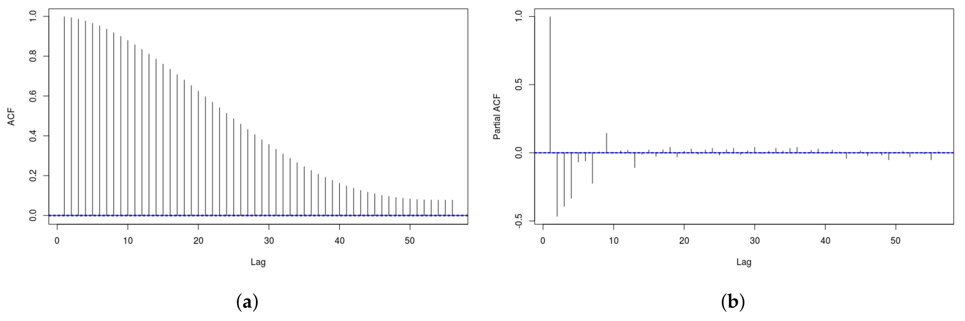
Figure 2.
Dataset pre-processing. w determines the amount of the historical data used, while h determines the prediction horizon.
Figure 2.
Dataset pre-processing. w determines the amount of the historical data used, while h determines the prediction horizon.

Figure 3.
An example scheme of stacking ensemble learning.

Figure 4.
A graphical representation of the ensemble scheme used in this paper. NN: Artificial Neural Network; RF: Random Forests; GBM: Generalized Boosted Regression Models.
Figure 4.
A graphical representation of the ensemble scheme used in this paper. NN: Artificial Neural Network; RF: Random Forests; GBM: Generalized Boosted Regression Models.
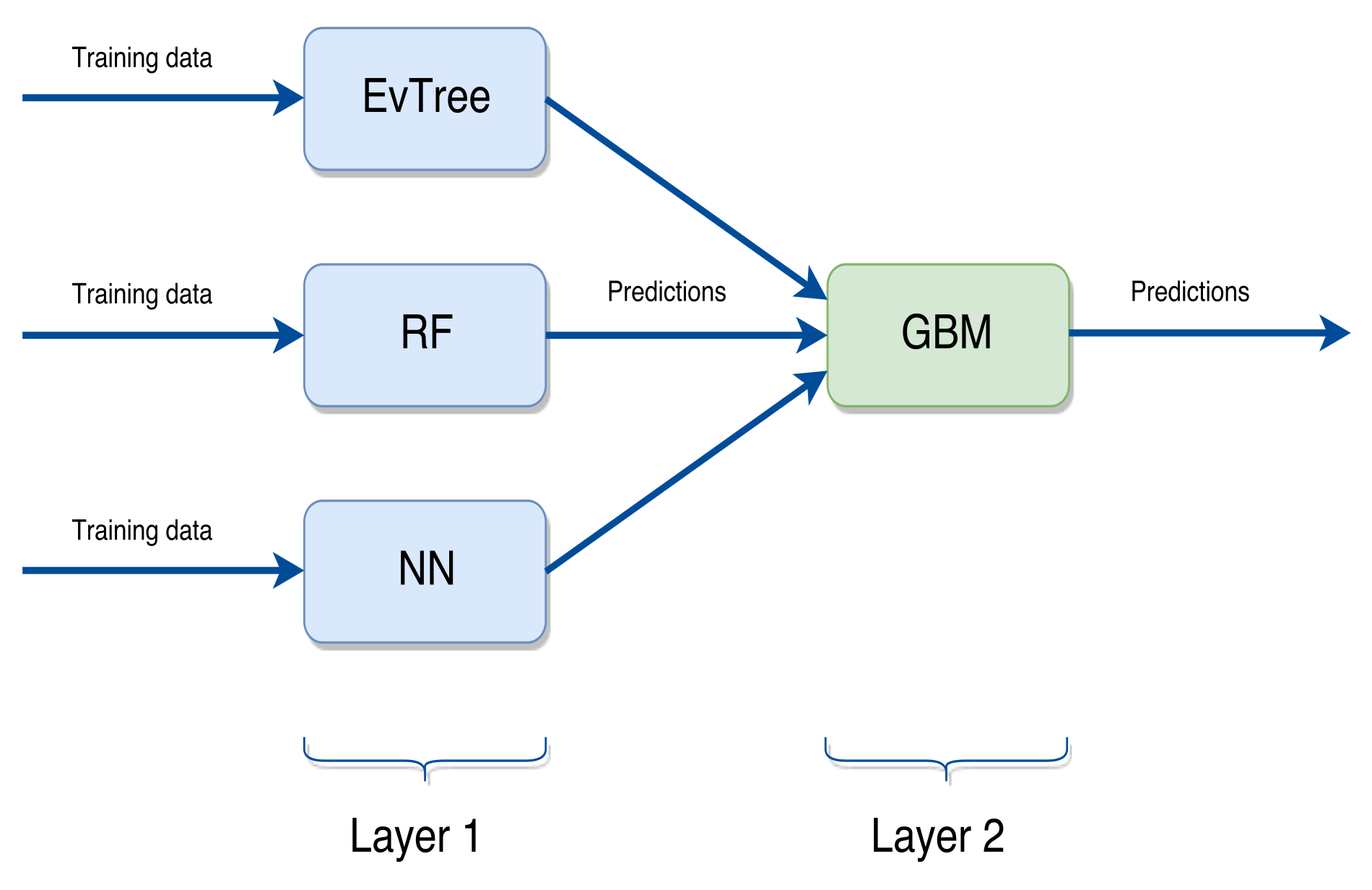
Figure 5.
A scheme of the ensemble learning strategy used in this paper. w determines the size of the historical window used, while h determines the prediction horizon.
Figure 5.
A scheme of the ensemble learning strategy used in this paper. w determines the size of the historical window used, while h determines the prediction horizon.
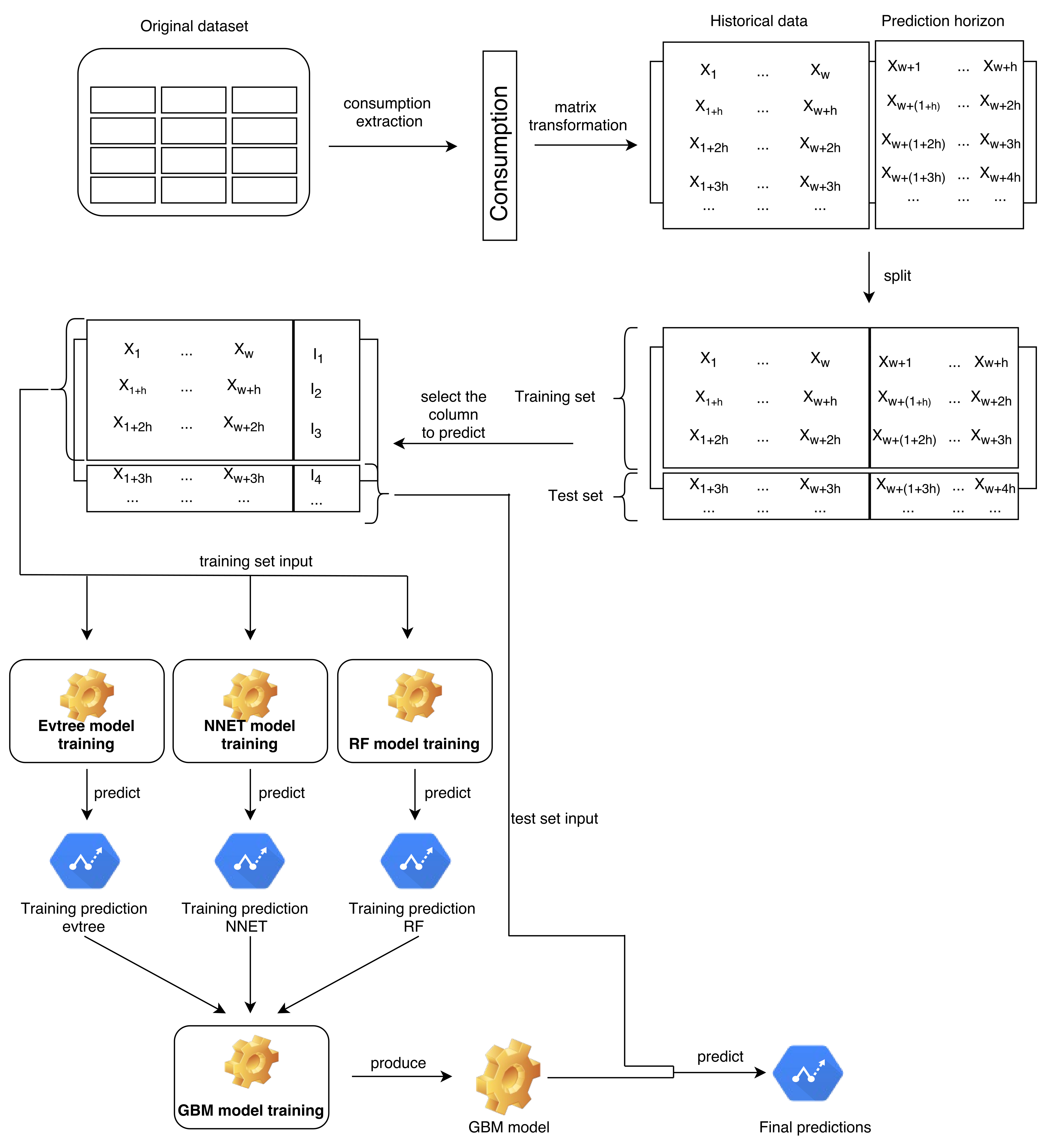
Figure 6.
Comparison of the MRE obtained by the base algorithms and the ensemble scheme on each subproblem for each value of w used. (a) w = 168; (b) w = 144; (c) w = 120; (d) w= = 96; (e) w = 72; (f) w = 48; (g) w = 24; (h) average MRE.
Figure 6.
Comparison of the MRE obtained by the base algorithms and the ensemble scheme on each subproblem for each value of w used. (a) w = 168; (b) w = 144; (c) w = 120; (d) w= = 96; (e) w = 72; (f) w = 48; (g) w = 24; (h) average MRE.
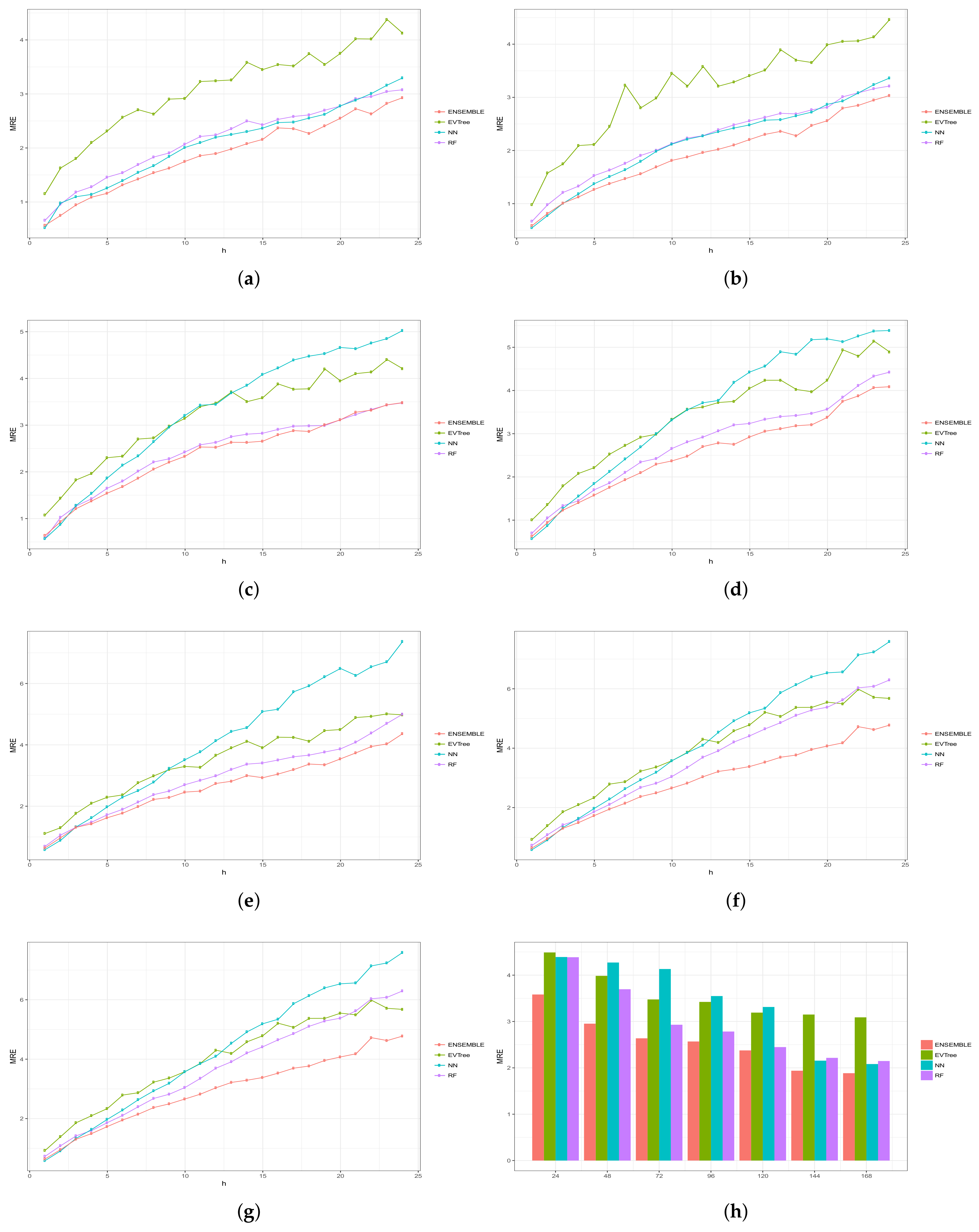
Figure 7.
Comparison of the MAE obtained by the base algorithms and the ensemble scheme on each subproblem for each value of w used. (a) w = 168; (b) w = 144; (c) w = 120; (d) w= = 96; (e) w = 72; (f) w = 48; (g) w = 24; (h) average MAE.
Figure 7.
Comparison of the MAE obtained by the base algorithms and the ensemble scheme on each subproblem for each value of w used. (a) w = 168; (b) w = 144; (c) w = 120; (d) w= = 96; (e) w = 72; (f) w = 48; (g) w = 24; (h) average MAE.

Figure 8.
Comparison of the R2 obtained by the base algorithms and the ensemble scheme on each subproblem for each value of w used. (a) w = 168; (b) w = 144; (c) w = 120; (d) w= = 96; (e) w = 72; (f) w = 48; (g) w = 24; (h) average R2.
Figure 8.
Comparison of the R2 obtained by the base algorithms and the ensemble scheme on each subproblem for each value of w used. (a) w = 168; (b) w = 144; (c) w = 120; (d) w= = 96; (e) w = 72; (f) w = 48; (g) w = 24; (h) average R2.
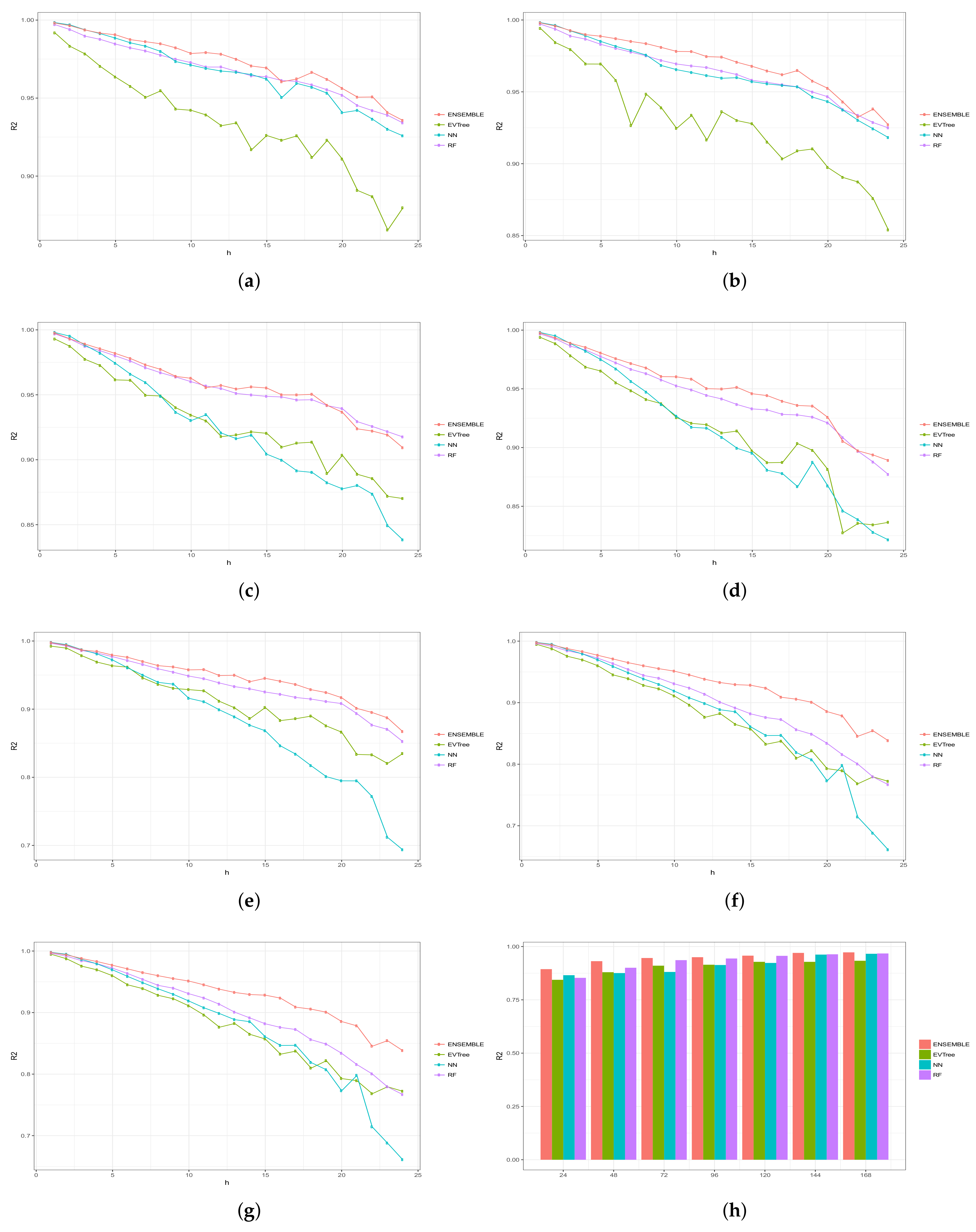
Figure 9.
Comparison of the sMAPE obtained by the base algorithms and the ensemble scheme on each subproblem for each value of w used. (a) w = 168; (b) w = 144; (c) w = 120; (d) w= = 96; (e) w = 72; (f) w = 48; (g) w = 24; (h) average sMAPE.
Figure 9.
Comparison of the sMAPE obtained by the base algorithms and the ensemble scheme on each subproblem for each value of w used. (a) w = 168; (b) w = 144; (c) w = 120; (d) w= = 96; (e) w = 72; (f) w = 48; (g) w = 24; (h) average sMAPE.

Figure 10.
Comparison of the RMSE obtained by the base algorithms and the ensemble scheme on each subproblem for each value of w used. (a) w = 168; (b) w = 144; (c) w = 120; (d) w= = 96; (e) w = 72; (f) w = 48; (g) w = 24; (h) average rMSE.
Figure 10.
Comparison of the RMSE obtained by the base algorithms and the ensemble scheme on each subproblem for each value of w used. (a) w = 168; (b) w = 144; (c) w = 120; (d) w= = 96; (e) w = 72; (f) w = 48; (g) w = 24; (h) average rMSE.

Figure 11.
Comparison of real and predicted values for a subset of the time serie, for . (a) 250 readings; (b) 1000 readings.
Figure 11.
Comparison of real and predicted values for a subset of the time serie, for . (a) 250 readings; (b) 1000 readings.
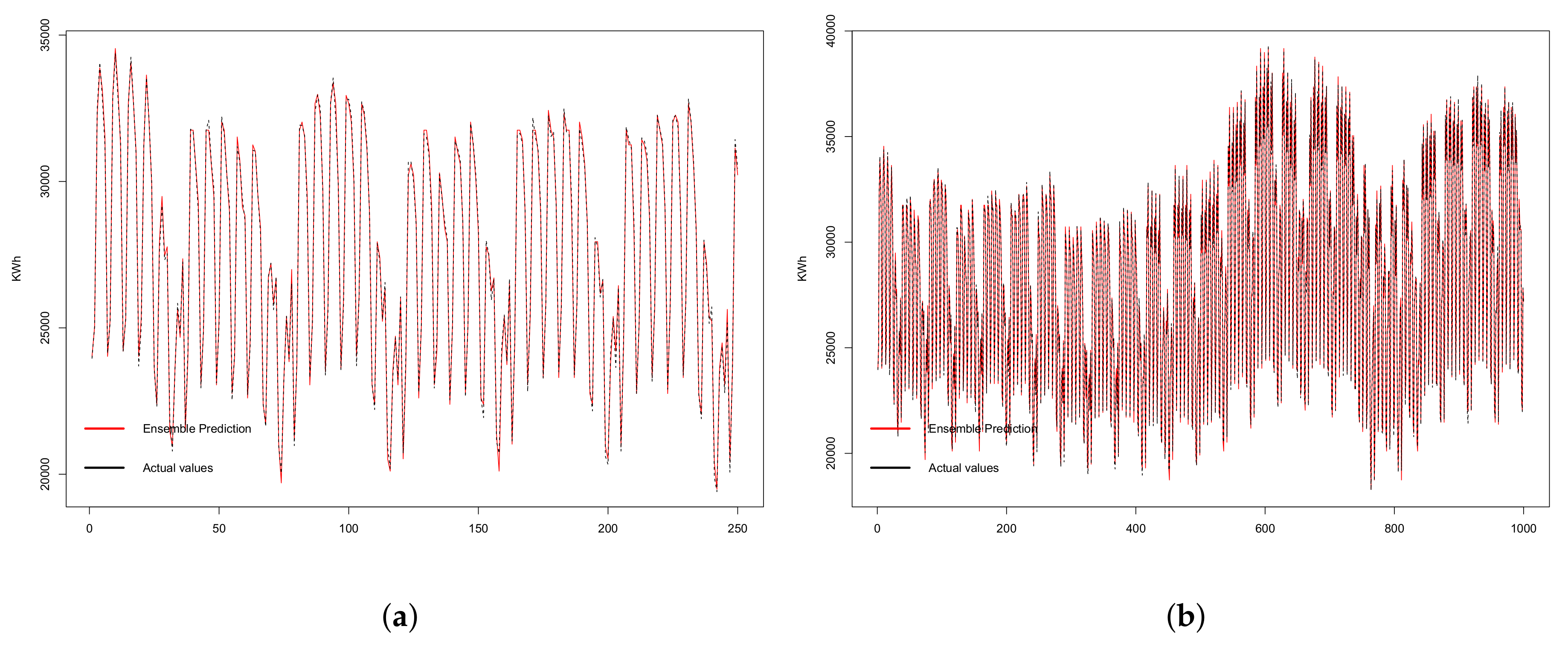
Table 1.
Dataset information depending on the value of w.
| w | #Rows | #Columns | File Size (In MB) |
|---|---|---|---|
| 24 | 20,742 | 48 | 6 |
| 48 | 20,741 | 72 | 9 |
| 72 | 20,740 | 96 | 11.9 |
| 96 | 20,739 | 120 | 14.9 |
| 120 | 20,738 | 144 | 17.9 |
| 144 | 20,737 | 168 | 20.9 |
| 168 | 20,736 | 192 | 23.9 |
Table 2.
Ranking of the methods according to their performances obtained on different values of w, according to the MRE.
Table 2.
Ranking of the methods according to their performances obtained on different values of w, according to the MRE.
| 168 | 144 | 120 | 96 | 72 | 48 | 24 |
|---|---|---|---|---|---|---|
| GBM | GBM | GBM | GBM | GBM | GBM | GBM |
| NN | NN | RF | RF | RF | RF | RF,NN,EV |
| RF | RF | NN,EV | NN,EV | EV | NN,EV | |
| EV | EV | NN |
Table 3.
Average results for different historical window values. Standard deviation between brackets.
Table 3.
Average results for different historical window values. Standard deviation between brackets.
| w | LR | ARMA | ARIMA | DL | DT | GBM | RF | EV | NN | ENSEMBLE | |
|---|---|---|---|---|---|---|---|---|---|---|---|
| 24 | MRE | 4.44 (2.27) | 7.67 (5.37) | 8.82 (5.31) | 4.51 (0.52) | 9.52 (1.55) | 8.07 (3.82) | 4.39 (2.13) | 4.49 (1.91) | 4.39 (2.23) | 3.58 (1.65) |
| 0.86 (0.11) | 0.56 0.45() | 0.50 (0.45) | 0.85 (0.03) | 0.52 (0.14) | 0.53 (0.37) | 0.85 (0.11) | 0.84 (0.11) | 0.87 (0.11) | 0.89 (0.08) | ||
| MAE | 1224.06 (613.04) | 2096.85 (1440.9) | 2335.87 (1339.15) | 1221.30 (153.89) | 2570.06 (419.80) | 2179.40 (1016.69) | 1200.82 (564.23) | 1232.31 (512.40) | 1212.29 (605.33) | 994.40 (450.33) | |
| RMSE | 1541.10 (731.72) | 2564.07 (1691.68) | 2854.95 (1596.35) | 1712.24 (229.01) | 3167.26 (507.99) | 2847.41 (1322.07) | 1619.18 (719.97) | 1686.17 (702.20) | 1530.60 (726.11) | 1373.46 (611.06) | |
| sMAPE | 0.04 (0.02) | 0.07 (0.05) | 0.08 (0.05) | 0.04 (0.01) | 0.09 (0.01) | 0.08 (0.04) | 0.04 (0.02) | 0.04 (0.02) | 0.04 (0.02) | 0.03 (0.02) | |
| 48 | MRE | 4.28 (2.15) | 8.67 (4.71) | 8.26 (4.73) | 3.46 (0.33) | 9.45 (1.48) | 6.59 (2.71) | 3.69 (1.71) | 3.98 (1.52) | 4.27 (2.16) | 2.95 (1.19) |
| 0.87 (0.10) | 0.42 (0.48) | 0.56 (0.39) | 0.92 (0.02) | 0.53 (0.13) | 0.71 (0.19) | 0.91 (0.07) | 0.88 (0.07) | 0.88 (0.10) | 0.93 (0.05) | ||
| MAE | 2416.92 (1306.55) | 2162.29 (1177.52) | 1183.61 (583.02) | 940.30 (68.74) | 2533.13 (402.45) | 1767.13 (722.83) | 683.95 (212.99) | 882.94 (258.51) | 914.31 (372.27) | 661.85 (220.79) | |
| RMSE | 3088.10 (1695.05) | 2673.49 (1451.80) | 1502.38 (702.01) | 1278.91 (96.08) | 3123.00 (484.50) | 2307.27 (938.98) | 1346.35 (559.10) | 1501.66 (569.11) | 1478.45 (686.62) | 1123.27 (448.52) | |
| sMAPE | 0.04 (0.02) | 0.09 (0.05) | 0.08 (0.04) | 0.03 (0.01) | 0.09 (0.01) | 0.07 (0.03) | 0.04 (0.02) | 0.04 (0.01) | 0.04 (0.01) | 0.03 (0.01) | |
| 72 | MRE | 4.20 (2.11) | 8.08 (4.54) | 11.37 (10.43) | 3.39 (0.30) | 9.33 (1.39) | 5.73 (2.23) | 2.93 (1.16) | 3.48 (1.18) | 4.13 (2.05) | 2.64 (0.99) |
| 0.88 (0.09) | 0.55 (0.43) | −0.07 (1.97) | 0.91 (0.02) | 0.54 (0.11) | 0.77 (0.15) | 0.94 (0.04) | 0.91 (0.05) | 0.88 (0.09) | 0.94 (0.03) | ||
| MAE | 1160.92 (568.26) | 2240.28 (1253.74) | 2964.83 (2665.97) | 933.16 (57.97) | 2501.64 (382.32) | 1554.40 (616.75) | 807.90 (311.53) | 958.09 (321.24) | 1135.84 (551.56) | 733.53 (274.41) | |
| RMSE | 1479.29 (680.59) | 2728.97 (1490.84) | 3562.36 (3098.46) | 1268.38 (70.18) | 3088.75 (457.78) | 2062.79 (819.53) | 1095.35 (402.20) | 1308.87 (450.01) | 1452.17 (664.60) | 1002.69 (372.10) | |
| sMAPE | 0.04 (0.02) | 0.08 (0.05) | 0.10 (0.08) | 0.03 (0.01) | 0.09 (0.01) | 0.06 (0.02) | 0.03 (0.01) | 0.03 (0.01) | 0.04 (0.02) | 0.03 (0.01) | |
| 96 | MRE | 3.57 (1.57) | 4.66 (1.81) | 14.03 (13.00) | 3.12 (0.42) | 9.40 (1.45) | 5.33 (2.08) | 2.78 (1.04) | 3.42 (1.15) | 3.55 (1.56) | 2.57 (0.97) |
| 0.91 (0.05) | 0.86 (0.08) | −0.79 (3.57) | 0.92 (0.02) | 0.53 (0.12) | 0.79 (0.13) | 0.94 (0.03) | 0.91 (0.05) | 0.91 (0.05) | 0.95 (0.03) | ||
| MAE | 989.02 (429.51) | 1264.58 (479.21) | 3689.22 (3335.65) | 852.76 (82.42) | 2522.55 (397.32) | 1461.03 (555.86) | 768.15 (278.34) | 942.47 (312.53) | 974.30 (420.29) | 714.16 (266.36) | |
| RMSE | 1279.62 (522.56) | 1619.73 (613.18) | 4562.39 (4075.72) | 1179.32 (114.33) | 3104.58 (472.31) | 1959.78 (735.49) | 1032.84 (358.21) | 1277.09 (431.31) | 1262.61 (513.00) | 969.66 (351.15) | |
| sMAPE | 0.04 (0.02) | 0.04 (0.02) | 0.12 (0.09) | 0.03 (0.01) | 0.09 (0.01) | 0.05 (0.02) | 0.03 (0.01) | 0.03 (0.01) | 0.04 (0.01) | 0.02 (0.01) | |
| 120 | MRE | 3.33 (1.37) | 5.21 (1.87) | 6.79 (2.53) | 2.98 (0.28) | 9.08 (1.12) | 5.02 (1.81) | 2.45 (0.79) | 3.19 (0.95) | 3.15 (1.41) | 2.38 (0.81) |
| 0.92 (0.05) | 0.84 (0.08) | 0.73 (0.14) | 0.94 (0.02) | 0.55 (0.10) | 0.81 (0.11) | 0.96 (0.02) | 0.93 (0.04) | 0.92 (0.05) | 0.96 (0.02) | ||
| MAE | 932.07 (381.65) | 1423.16 (499.93) | 1858.88 (682.36) | 814.90 (48.48) | 2440.62 (330.11) | 1368.47 (477.79) | 683.95 (212.99) | 882.94 (258.51) | 914.31 (372.27) | 661.85 (220.79) | |
| RMSE | 1215.03 (475.89) | 1758.60 (623.36) | 2282.80 (817.39) | 1094.97 (72.06) | 3047.58 (430.15) | 1857.81 (655.27) | 920.01 (287.27) | 1184.92 (354.34) | 1197.00 (464.15) | 905.00 (300.87) | |
| sMAPE | 0.03 (0.01) | 0.05 (0.02) | 0.07 (0.03) | 0.03 (0.01) | 0.09 (0.01) | 0.05 (0.02) | 0.02 (0.01) | 0.03 (0.01) | 0.03 (0.01) | 0.02 (0.01) | |
| 144 | MRE | 2.15 (0.77) | 2.57 (0.91) | 7.63 (2.54) | 2.32 (0.29) | 8.86 (1.01) | 4.49 (1.54) | 2.22 (0.71) | 3.15 (0.90) | 2.16 (0.78) | 1.94 (0.69) |
| 0.96 (0.02) | 0.95 (0.03) | 0.66 (0.17) | 0.96 (0.01) | 0.57 (0.09) | 0.85 (0.09) | 0.96 (0.02) | 0.93 (0.03) | 0.96 (0.02) | 0.97 (0.02) | ||
| MAE | 589.62 (211.22) | 712.61 (247.39) | 2048.65 (653.32) | 624.32 (54.92) | 2366.77 (403.55) | 1220.77 (403.55) | 608.67 (188.85) | 866.84 (244.39) | 589.27 (211.57) | 530.28 (184.26) | |
| RMSE | 845.03 (302.78) | 969.86 (335.40) | 2579.71 (835.12) | 852.89 (85.96) | 2966.20 (355.50) | 1694.63 (574.47) | 837.13 (269.50) | 1184.39 (352.66) | 845.01 (303.06) | 745.31 (278.77) | |
| sMAPE | 0.02 (0.01) | 0.03 (0.01) | 0.07 (0.02) | 0.02 (0.01 | 0.08 (0.01) | 0.04 (0.02) | 0.02 (0.01) | 0.03 (0.01) | 0.02 (0.01) | 0.02 (0.01) | |
| 168 | MRE | 2.07 (0.77) | 2.43 (0.97) | 6.92 (2.97 ) | 2.46 (0.29) | 8.79 (0.96) | 4.45 (1.56) | 2.15 (0.69) | 3.09 (0.84) | 2.08 (0.74) | 1.88 (0.67) |
| 0.97 (0.02) | 0.96 (0.03) | 0.71 (0.19) | 0.96 (0.01) | 0.58 (0.08) | 0.85 (0.09) | 0.97 (0.02) | 0.93 (0.03) | 0.97 (0.02) | 0.98 (0.02) | ||
| MAE | 562.39 (209.83) | 660.20 (261.58) | 1836.62 (757.95) | 661.24 (51.93) | 2386.25 (296.70) | 1712.81 (611.79) | 585.67 (182.05) | 847.30 (226.72) | 571.54 (217.91) | 513.50 (181.09) | |
| RMSE | 785.84 (296.05) | 889.18 (356.54) | 2332.30 (965.02) | 901.78 (84.22) | 2988.47 (370.41) | 1712.81 (611.78) | 792.58 (303.12) | 1145.55 (324.05) | 795.58 (303.12) | 714.56 (266.00) | |
| sMAPE | 0.02 (0.01) | 0.02 (0.01) | 0.07 (0.02) | 0.02 (0.01 | 0.08 (0.01) | 0.04 (0.02) | 0.02 (0.01) | 0.03 (0.01) | 0.02 (0.01) | 0.02 (0.01) |
© 2018 by the authors. Licensee MDPI, Basel, Switzerland. This article is an open access article distributed under the terms and conditions of the Creative Commons Attribution (CC BY) license (http://creativecommons.org/licenses/by/4.0/).
Share and Cite
MDPI and ACS Style
Divina, F.; Gilson, A.; Goméz-Vela, F.; García Torres, M.; Torres, J.F. Stacking Ensemble Learning for Short-Term Electricity Consumption Forecasting. Energies 2018, 11, 949. https://doi.org/10.3390/en11040949
AMA Style
Divina F, Gilson A, Goméz-Vela F, García Torres M, Torres JF. Stacking Ensemble Learning for Short-Term Electricity Consumption Forecasting. Energies. 2018; 11(4):949. https://doi.org/10.3390/en11040949
Chicago/Turabian StyleDivina, Federico, Aude Gilson, Francisco Goméz-Vela, Miguel García Torres, and José F. Torres. 2018. "Stacking Ensemble Learning for Short-Term Electricity Consumption Forecasting" Energies 11, no. 4: 949. https://doi.org/10.3390/en11040949
Note that from the first issue of 2016, this journal uses article numbers instead of page numbers. See further details here.