A High-Efficiency Charging Service System for Plug-in Electric Vehicles Considering the Capacity Constraint of the Distribution Network

Abstract

It takes electric vehicles (EVs) a long time to charge, which is bound to influence the charging experience of vehicle owners. At the same time, large-scale charging behavior also brings about large load pressure on, and elevates the overload risk of, the power distribution network. To solve these problems, we proposed a high-efficiency charging service system based on charging reservation and charging pile binding services. The system can shorten the average charging time of EVs and improve the average immediate utilization rate of new energy sources at charging stations (CSs). In addition, the system also guarantees that the EVs are charged within the allowable range of the capacity of the distribution network and avoids overloading of the distribution network caused by the charging of EVs. The key support for the utility of the system is rooted in the three-level CS selection model and the CS energy control algorithm (CSECA) proposed in the research. Finally, the proposed model and algorithm were verified to be valid through numerous simulation experiments.

1. Introduction

As environmental pollution and oil resource availability become increasingly prominent issues, electric vehicles (EVs), as alternatives to oil-fueled vehicles, have attracted worldwide attention. In recent years, the power batteries mounted on EVs have witnessed rapid development and the driving range of the EVs has also increased to now allow mid-long-distance journeys. In such a context, it is inevitable that en route EV charging occurs [1,2]; however, conventional public EV charging equipment mainly provides a slow charging service and it generally takes up to 6–8 h to charge an EV [2], which is inconvenient. While, vehicle owners have become used to the rapid refueling of oil-fueled vehicles, so it is hard for them to adapt to the slow charging regime of an EV [3]. Therefore, developing a high-efficiency EV charging service to shorten the waiting time is a feasible step to take when trying to solve this problem.

At present, numerous studies have been carried out to investigate high-efficiency charging of EVs and these studies can be divided into two types: high-efficiency charging of EVs used for intercity transport and high-efficiency charging of urban EVs, which take the charging of EVs driving on highways or inside a city as objects, respectively.

Two highway charging models were proposed in [4], and they are based on local information about the EVs and interactive information between global CS-selection (GCS) and EVs. Simulation results indicated that the two models can effectively shorten the waiting time for charging of EVs on highways. In [5], an intelligent EV charging schedule method based on the A* algorithm and a point-to-point EV scheduling system was developed and the method arranges the charging plans of EVs by assessing the real-time status of EV charging stations (CSs) to shorten the overall travel time of EVs. In [6,7], a method for regulating the queue for EVs waiting to be charged at highway EV CSs based on queuing theory was proposed. The method reduces the waiting time of EVs and improves the overall utilization rate of highway CSs by dispatching EVs needing to be charged to CSs with a high queue limit. In [8], the authors utilized railway infrastructures to supply the charging power of EVs in highways.

Three strategies based on EV charging price were proposed in [9] to arrange EVs that need charging in cities on a dynamic basis. The strategies can not only reduce the charging cost of EVs but also are able to boost the overall profit of the CSs. In [10], the framework for an EV cooperative charging agreement suitable for residential areas was proposed to solve the problem that an EV parking space for charging was occupied by an EV that had been fully charged and to help EVs needing charging to find available parking spaces for charging. An intelligent machine learning algorithm was put forward to help EV owners to find charging piles that can be used upon arrival to shorten the time needed to look for charging piles and the waiting time [11]. A high-efficiency charging system was proposed in [12] to serve the EVs that need to be recharged in the trip. The system highlights the charging management of EVs and can shorten the average waiting time for EV charging. In [13], the management strategies for charging of EVs during the parking lots were proposed, which can minimize the power losses on distribution system and the cost of purchased energy.

The above studies are all based on the assumption that the capacity of the distribution network is able to satisfy the charging demand of all EVs while ignoring the influences of capacity constraint of the distribution network: however, numerous studies have revealed that the large-scale charging of EVs can increase the load pressure on the distribution network, such as the increases in power losses [14], voltage deviations [15] and peak load [16]. If such large-scale charging behavior is not controlled, local overloading of the distribution network is likely to occur in peak load periods [17]. Guiding EVs to be charged in an optimally ordered fashion can decrease the peak load on the power grid and therefore achieve the aim of peak clipping [18,19]. Among existing methods, the guidance method of EV charging based on charging price is widely used to control the charging of EVs. In [20], two valley-filling pricing mechanisms were proposed to incent EV owners to charge their EVs during valley load period and the results proved the efficacy of the mechanisms. The authors proposed a pricing strategy based on the actual load on the grid for controlling the charging of EVs, which can minimize transmission costs in the distribution grid [21]. In [22], a multi-objective optimization framework that can set the retail charging price for the charging service provider was proposed and the simulation results show that the price can decrease the load pressure on the grid. In [23], the authors used time-of-use (TOU) power price to guide the charging of EVs for reducing charging cost and the power network loss rate and the results proved its effectiveness. In these methods, users determine whether to charge their EVs or not according to price and the method places emphasis on the orderly guidance of EVs in terms of time. However, the control effect of the method is sensitive to the degree of participation of EV owners and a low degree of participation is likely to decrease the control effect. Different from the guidance method based on electricity price, an EV charging strategy based on the on-off mechanism was proposed in [24]. According to the method, the charging behavior is not determined by EV owners but by the output result of the centralized charging algorithm after connecting EVs with charging equipment. The charging equipment comes under on-off control according to the results of the algorithm. The strategy can control the charging load of EVs and reduce the operating pressure on the power grid. However, the charging behavior is wholly determined by the control algorithm which ignores the feelings of EV owners, which influence the charging experience of users, especially under conditions in which EVs need to be charged as a matter of urgency.

The research focused on high-efficiency charging of EVs in cities. Differing from previous research, we designed a high-efficiency charging system for EVs in cities by combining the orderly guidance and control of EV charging: the system framework is shown in Figure 1. The system is composed of four parts: (1) charging demand transfer platform (CDTP); (2) smart grid OMS (SGOMS); (3) charging management platform (CMP); and (4) CS energy controller (CSEC). The information exchange among these four parts is realized over the Internet. The system provides real-time charging reservation, CS selection, and charging pile binding services. By using the system, an EV owner only need apply for charging reservation by using mobile networks while driving. Afterwards, the system helps the owner to search for an optimal CS for selection by the owner and binds a charging pile at the CS before the owner makes the selection decision, so as to avoid the charging pile being occupied by another EV before the owner makes a decision, and to guarantee that the EV applying for charging reservation can be charged upon arrival. The optimal CS is determined by using the three-level CS selection model proposed in the research, and the model is applicable to conventional grid-connected CSs and grid-connected CSs that contain new energy sources and energy storage. Differing from the orderly guidance model in terms of the time, the CS selection model is designed to realize the orderly guidance of EV charging in a spatial domain and is based on the assumption that the charging price at a CS is not determined at the discretion of single CS operators but by a unified pricing agency. In addition, the CSs within the same service area adopt the same charging price, which is known as the charging price of a service area, and different service areas have disparate charging prices. It was proposed in [25] that the CO₂ emissions of an EV are higher than those of an equivalent oil-fueled vehicle if the electricity used by the EV mainly comes from the thermal power plant that applies coal as its primary energy. Obviously, if as much electricity as is used by the EV derives from new energy sources, it can reduce the possibility, and even avoid the occurrence, of the above situation. Therefore, improving the average immediate utilization rate of new energies in service areas of the system is also taken as an aim of the model. Moreover, to improve the charging efficiency and reduce anxiety among EV owners, we also apply the reduction of the average waiting time for EV charging as an aim of the model. As to the EV charging control, we assume that the EVs in service areas of the proposed high-efficiency EV charging service system have achieved scale development. In addition, it is assumed that the capacity of the distribution network in an area is limited, so the charging of EVs needs to be controlled to some extent. Considering this, we also came up with a CSECA. It is worth noting that the algorithm uses the first-in/first-out (FIFO) charging rule (EVs arriving earlier at a CS preferentially obtain the optimal charging power) as the premise from which obtain maximum utility. By using the algorithm, the distribution network load of CSs can be maintained within the allowable range, thus avoiding the overloading of the distribution network caused by EV charging. Given this precondition, the EV charging demand at a CS can be met to maximum effect. For the CSs containing energy storage battery (ESB), the algorithm guarantees that the state of charge (SoC) and output of the ESB are within the allowable working range. The remainder of the paper is arranged as follows: Section 2 introduces the design and communication frameworks of the proposed high-efficiency EV charging service system; Section 3 explains the service rules of the system and then describes the three-level CS selection model, as well as the aims and meanings of each level. Finally, the section elaborates the CSECA algorithm, including the control aims and means of the algorithm; Section 4 verifies the proposed model and algorithm through simulation; and Section 5 draws conclusions from the research.

2. System Framework

The CDTP is mainly responsible for receiving the charging demand from EV owners by the GPRS/4G and sends the information across the Internet to specific CMPs for distributed processing. After receiving the charging demand information from EV owners, the CMP intelligently selects a CS according to the day-ahead charging power constraints of CSs and the real-time CS information sent over the Internet by the CSEC. This not only guarantees the high-efficiency charging experience of EV owners but also improves the average immediate utilization rate of new energy sources at CSs in the service area. The CSEC manages the energy in CSs according to the day-ahead charging power constraint sent by the CMP, and real-time CS information, to ensure that the sum of loads of all CSs in the high-efficiency charging service areas is within the range of the day-ahead EV charging plan, thus realizing the aim of reducing the overload risk in the distribution network.

2.1. Assumption

We assume that the EVs have gained large-scale development in the high-efficiency charging service areas. EV owners can apply for charging reservations to the CDTP while driving, or when parking, and send charging demand information, including the locations of EVs, residual mileage, vehicle identification number (VIN), rated charging power, and amount of electricity needed. Afterwards, EV owners will receive the demand response from the CDTP, which includes the name of the selected CS, serial number of the charging pile, and charging time. In addition, the SGOMS can offer the day-ahead charging power constraint of each area and sends it to the CMP for the corresponding area. The CMP transforms the received information to the day-ahead charging power constraints for each CS around responsibility and transmits the information to its corresponding CSEC in an end-to-end way. After receiving the information, the CSEC saves it to its own database.

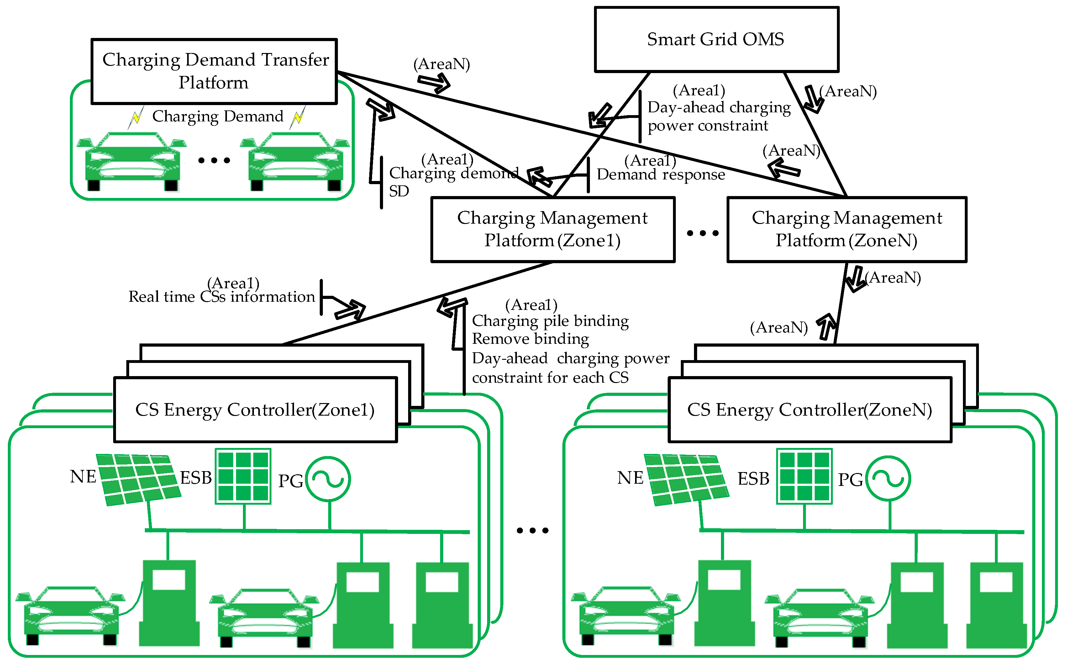
2.2. Distributed Design

With the scale development of EVs, the amount information pertaining to charging demand also grows. If centralized processing is used to deal with such a large amount of information [26,27], it will increase the hardware investment cost of the overall system, and even influences the efficiency of operation thereof. Distributed processing of information can solve this problem. To realize distributed processing, we divide the service area of the whole system into several small areas (Areas 1 to N), in each of which a CMP is deployed to govern the charging service for the area. These CMP are mutually independent and each one only receives charging service information (charging demand and service dissatisfaction (SD)), real-time CS information, and the day-ahead charging power constraint for the area sent by the SGOMS within the area of its responsibility.

2.3. Communication Framework

The proposed high-efficiency EV charging service system has the same communication framework in each service area. Taking the charging reservation of an EV in Area 1 as an example, the section describes the communication framework, as shown in Figure 2.

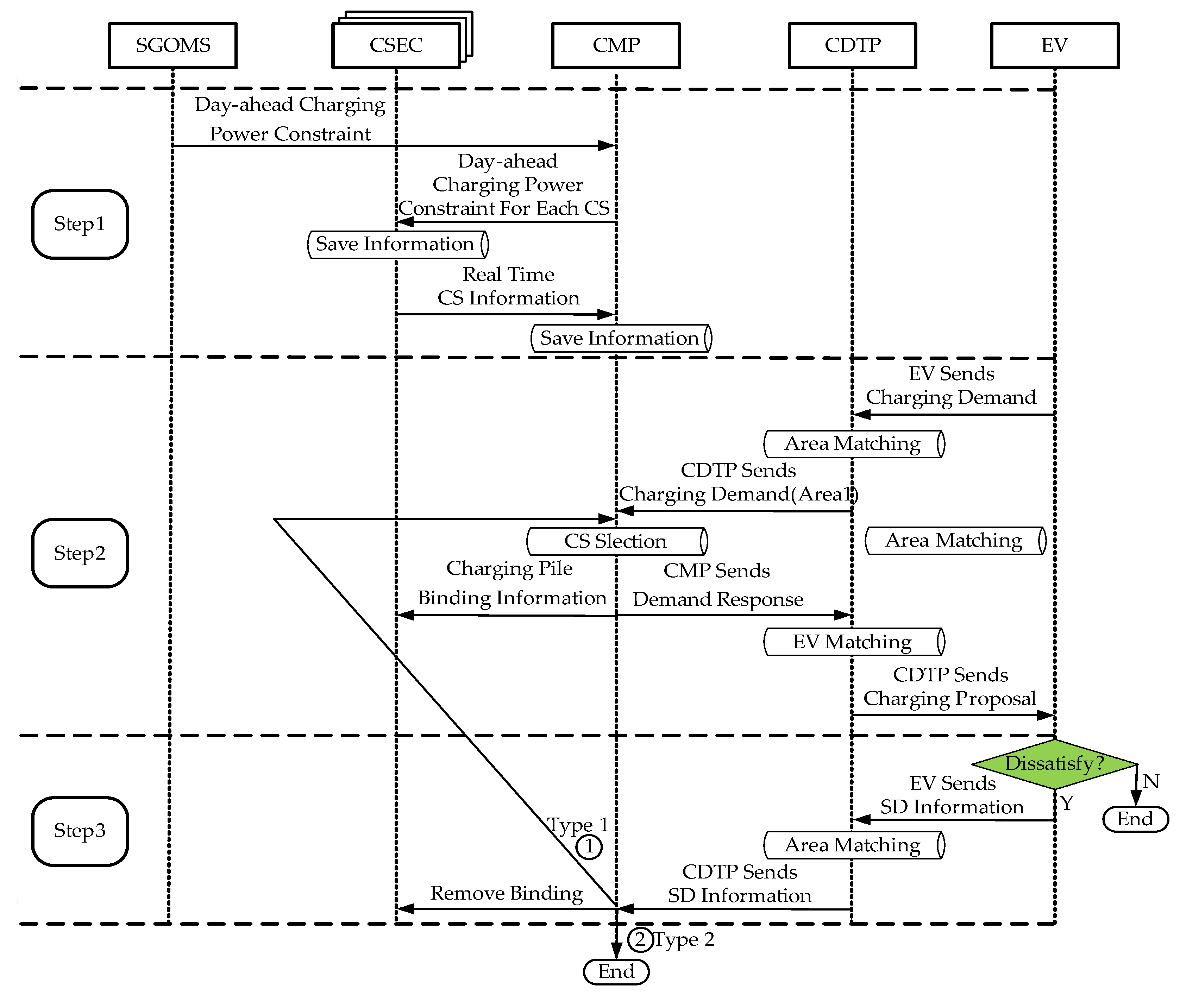
• Step 1: the SGOMS sends the day-ahead charging power constraint of the area which the CMP is responsible for to the CMP. Then, the CMP transforms the information to the day-ahead charging power constraints for each CS around responsibility and sends the information to the corresponding CSEC in an end-to-end manner. The CSEC saves the information. As the status of the CSs is influenced by the random access, or departure, of EVs, the status information of CSs also changes at random. Therefore, to reduce the influences of such randomness on CMP computations, the CSEC will periodically send real-time CS information to the CMP. After receiving the information, the CMP saves it to its database.
• Step 2: the EV owner applies for a charging reservation to the CDTP which performs area matching for the reservation information and transmits the charging demand to the CMP which is responsible for the charging service of the area within which the EV is located. The CMP selects a CS and then sends the selection result as the demand response to the CDTP which transmits the information to the EV owner. After receiving the response, the EV owner can choose to go to the recommended CS for charging according to the response information and then the service ends or chooses to reject the recommendation or cancel it en route. In case of the latter, it turns to Step 3: in addition, to guarantee that the EV can be successfully charged after arriving at the recommended CS, the CMP sends the charging pile binding information to the CSEC in charge of the recommended CS while sending the charging proposal. The CSEC binds the assigned charging pile after receiving the instruction. It is worth noting that, once a charging pile is bound, it only provides service to the assigned EV until such binding is removed.
• Step 3: the EV owner sends the SD information to the CDTP which transmits that information to the CMP. Here, the SD information can be divided into two types: instructions 1 and 2 which correspond to the two selections of the EV owner: needing the system to find another CS or no longer needing service from the system. On receiving instruction 1, the CMP turns to the CS selection link in Step 2 and fulfils the residual links of Step 2. On receiving instruction 2, the CMP immediately stops providing service to the EV owner. No matter which instruction the CMP receives, it will send that instruction to the CSEC responsible for the recommended CS to remove the binding. After receiving the instruction, the CSEC immediately removes the binding of the assigned charging pile, so that the charging pile can be used by another EV.

3. Problem Formulation

3.1. Charging Reservation Rules

The EV owner as the initiator of charging demand needs to accomplish the following two operations: (1) sending a charging reservation to the CDTP and offering reservation information and (2) making decisions (agreement or denial) according to the demand response information. As mentioned above, the system binds a charging pile at the recommended CS at first to avoid the charging pile being used by other EVs, which thus benefits the EV owner sending a charging reservation; however, if the EV owner neither goes to the assigned charging pile for charging all the time, nor sends SD information to the system, the charging pile will always be bound and cannot provide a service to other EVs, thus bringing about a loss to the CS. To avert this situation, the following two charging reservation rules are formulated:

• Rule 1: the EV owner is expected to accomplish the second operation (making decisions) in a contracted response time, the starting moment of which is the moment when the EV owner receives the charging demand response. If the operation time exceeds the response time, the vehicle intelligent terminal (VIT) will automatically send the SD information containing instruction 2 to the system to terminate the charging service.
• Rule 2: on the condition that Rule 1 is not broken, the EV owner needs to arrive at the assigned charging pile to charge within the contracted time T^con. The EV owner is aware of the time before the reservation and T^con starts from the time when the EV owner receives the charging demand response. If the EV is not charged by the charging pile within T^con, the binding on the charging pile is removed.

3.2. Optimal Charging Demand Model of EVs

The queue and waiting time for EV charging, the charging price, and the traffic condition of the road to the CS are major criteria from which the EV owner can decide whether to charge the EV at the CS or not. In this research, it was supposed that the EV owner is aware of the charging prices in each service area before charging, so it implies that the EV owner accepts the charging price of a service area if they apply for a charging reservation therein. For this reason, the influence of the charging price on the CS selection of the EV owner can be ignored. Therefore, only the waiting time for EV charging and the traffic conditions along the route to the CS need be considered. The waiting time of the ith EV for charging at the jth CS can be expressed as

$$T_{ij}^{\mathrm{cha}}=(\arg \min \left|\frac{1}{60}\cdot {\displaystyle {\int }_{t_{ij}}^t{P}_{ij}^{\mathrm{cha}}(u)du}-E_i^{\mathrm{cha}}\right|-t_{ij})$$

(1)

where T_ij^cha stands for the time taken for charging the ith EV at the jth CS. The variable t_ij is the starting time for charging the ith EV (min). P_ij^cha(u) is actual charging power of the ith EV at the jth CS at time step u. E_i^cha is the amount of electricity obtained by the ith EV through charging. As to the traffic conditions along the route to the CS, it is represented by the time taken T_ij^travel by the ith EV for driving to the jth CS. Owing to T_ij^travel having the same dimension as the result of Equation (1), they are combined and the result is defined as the waiting time for charging and is expressed as follows

$$T_{ij}^{\mathrm{wait}}=T_{ij}^{\mathrm{cha}}+T_{{}_{ij}}^{\mathrm{travel}}$$

(2)

The moment when the ith EV arrives at the jth CS can be considered as

$$t_{ij}=T_{ij}^{\mathrm{travel}}+t_i^{\mathrm{res}}$$

(3)

where t_i^res stands for the moment when the ith EV applies for charging reservation. An EV owner would prefer a lower value result from Equation (2), in addition, the EV owner is not willing to go to a CS too far away from the current position of the EV or along a route experiencing congestion; i.e., there are a critical distance and a critical travel time, which are defined as the maximum distance D_i^max and travel time T_max^travel that can be accepted by EV owners. Suppose that they are constants, then the optimal charging demand of the EV can be represented as

$$\min T_{ij}^{\mathrm{wait}}$$

(4a)

$$s.t.\begin{array}{c}\end{array}{D}_{ij}\le \min [D_i^{\max },D_i^{\mathrm{re}}]$$

(4b)

$$T_{{}_{ij}}^{\mathrm{travel}}\le T_{\max }^{\mathrm{travel}}$$

(4c)

where D_ij is the Distance that the ith EV drives to the jth CS through the optimal path (km).

3.3. Three-Level CS Selection Model

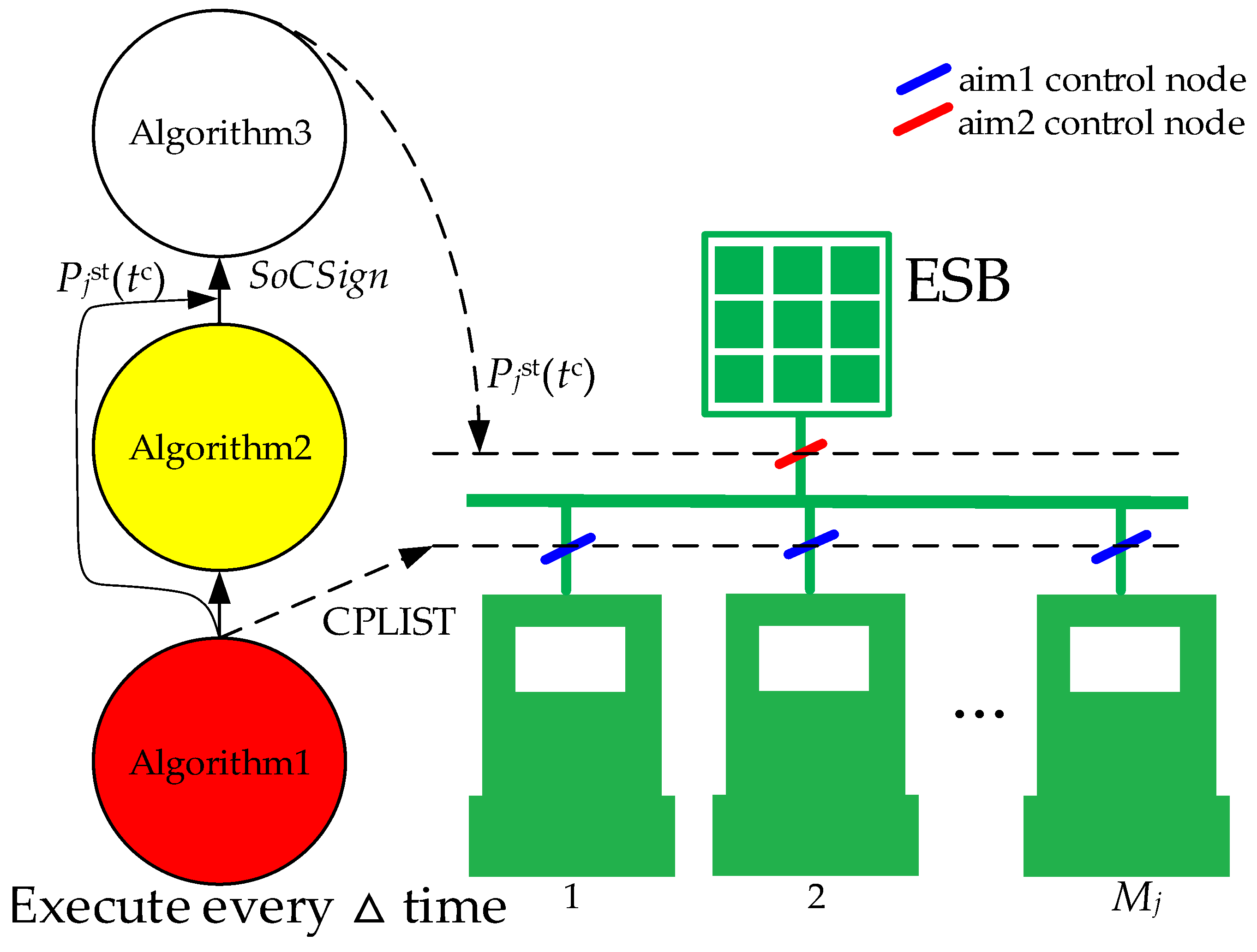
The section corresponds to the CS selection link in Figure 2 and aims to help the EV owner to search for a CS which has an idle charging pile in the vicinity by using the proposed three-level CS selection model. To begin with, we build a unified three-level CS selection model for two typical types of CSs: grid-connected CSs that contain new energy sources, and energy storage, and conventional grid-connected CSs. The mathematical expression of the first level is

$$\begin{array}{c}\mathrm{target}: J_i^{\mathrm{level}1}=\left\{j\right| j\in J^h,D_{ij}\le \min [D_i^{\max },D_i^{\mathrm{re}}],\\ T_{ij}^{\mathrm{travel}}\le T_{\max }^{\mathrm{travel}},{\alpha }_j=1\}\end{array}$$

(5a)

$${\alpha }_j=\{\begin{array}{l}1,\mathrm{if} \mathrm{there} \mathrm{is} \mathrm{an} \mathrm{idle} \mathrm{charging} \mathrm{pile} \mathrm{in} \mathrm{CS} j\\ 0,\mathrm{el}\mathrm{se} \end{array}$$

(5b)

where Equation (5a) represents the selection aim of the first level, which indicates that a set J^level1 of CSs satisfying Equations (4b) and (4c) and having an idle charging pile is initially sought from J^h standing for the set of CSs in the hth area. The aim not only guarantees that the selected CS can satisfy the charging demand constraints of the EV owner, that is, Equations (4b) and (4c), but also ensures that the selected CS has an idle charging pile for the EV owner. In this way, the idle charging piles near the EV can be made full use of and it avoids the occurrence of the situation where EV owners go to CSs without idle charging piles and therefore must wait. This is beneficial to reducing the waiting time, and besides, combining with the charging pile binding service of the service system, it can be guaranteed that the EV is charged as soon as it arrives at the CS. The mathematical expression for the second level of the selection model is

$$\mathrm{target}: J_i^{\mathrm{level}2}=\left\{j\right|j=\arg \min {\lambda }_i^1(j)\}\cup \{j|j=\arg \min {\lambda }_i^2(j)\}\dots \cup \left\{j\right|j=\arg \min {\lambda }_i^Q(j)\}$$

(6a)

$${\lambda }_i^q(j)={\sigma }_1\cdot \frac{T_{ij}^{\mathrm{travel}}}{T_{\max }^{\mathrm{travel}}}+{\sigma }_2\cdot {\delta }_{ij}\cdot G_{ij},j\in J_q^{\mathrm{level}1},q=1,2,3\dots$$

(6b)

$${\delta }_{ij}=\frac{1}{N_i-N_{ij}}{{\displaystyle \cdot \sum }}_{n=N_{ij}}^{N_i}\min [\frac{P_j^{\mathrm{CSL}}\left(n\right)+P_{ij}^{\max }}{P_j^{\mathrm{NE}}(n)},1]$$

(6c)

$$G_{ij}={{\displaystyle \sum }}_{n=N_{ij}}^{N_i}\frac{P_j^{\mathrm{CSL}}\left(n\right)+P_{ij}^{\max }}{(N_i-N_{ij})\cdot W_j\left(n\right)}$$

(6d)

$$W_j\left(n\right)=\{\begin{array}{l}\min [P_j^{\mathrm{grid}}\left(n\right)+P_j^{\mathrm{NE}}(n)+P_j^{\mathrm{s}},P_j^{\mathrm{rated}}], \mathrm{if} P_j^{\mathrm{grid}}\left(n\right)<P_j^{\mathrm{rated}}\&\&n\in [N_{ij},N_i]\\ P_j^{\mathrm{rated}},\mathrm{else} \mathrm{if} n\in [N_{ij},N_i]\end{array}$$

(6e)

$$P_j^{\mathrm{s}}=\min [\frac{60\cdot (So{C}_j(t_i^{\mathrm{res}})-So{C}_j^{-})\cdot E{S}_j}{N_i-N_{ij}},P_{{}^j}^{\mathrm{s}+}]$$

(6f)

$$P_j^{\mathrm{CSL}}\left(n\right)={\displaystyle \sum _{l=1}^{M_j}{\epsilon }_l\cdot P_{lj}^{\max }\cdot (u(n-N_{lj})}-u(n-N_{lj}^{\mathrm{d}}))$$

(6g)

$$T_i^{\mathrm{Icha}}=60\cdot \frac{E_i^{\mathrm{cha}}}{P_i^{\max }}$$

(6h)

$$J_q^{\mathrm{level}2}=\left\{j\right|\mathrm{if}\forall j_1,j\in J_q^{\mathrm{level}2},then{P}_{ij}^{\max }=P_{i{j}_1}^{\max }\}$$

(6i)

$$N_i=\lceil T_i^{\mathrm{Icha}}+T^{\mathrm{con}}+t_i^{\mathrm{res}}\rceil$$

(6j)

where u(^.) in Equation (6g) is a switch function. P_j^grid(n) and Pj^NE(n) stand for power constraint of the distribution network of the jth CS and predictive value of new energy of the jth CS in the nth time period, respectively. N_i is the optimal charging end-time of the ith EV, which can be obtained by Equation (6j). N_ij is integer value of t_ij. M_j is the number of EVs being charged at jth CS. P_j^s is equivalent output of energy storage at the jth CS in time period [N_ij, N_i]. P_j^s+ and ES_j stand for maximum output power of the energy storage and energy storage capacity of the jth CS, respectively. SoC_j(n) is SoC of energy storage at jth CS in the n time. SoC_j⁻ is minimum SoC of energy storage at the jth CS. T_i^Icha is optimal charging time of the ith EV at the jth CS, which can be calculated using Equation (6h). ε_l is shielding coefficient of the lth EV; 0 and 1 represent shielded and unshielded, respectively. P_ij^max is maximum charging power available to the ith EV charged at the jth CS. We partition the J^level1 into {J₁^level1, J₂^level1, …} using the partition rule. That is, the CSs which have same P_ij^max of the ith EV are classified into one type. Equation (6b) is the optimal evaluation function of the same type of CSs and the evaluation criterion is that, the smaller the function value, the better. The first term evaluates T_ij^travel, while σ₁ is the corresponding weight coefficient used to represent the weight of the term in the overall evaluation: the smaller T_ij^travel is, the smaller the term, which implies that the shorter the time that the EV owner takes for the trip, the higher the possibility of meeting the demand of charging as nearby as possible. The second term is to evaluate the CSs in the time period [N_ij, N_i], which focuses on the immediate utilization rate δ_ij of new energies at CSs and the power congestion G_ij of CSs. δ_ij can be calculated using Equation (6c), where P_j^CSL(n) is optimal load at the jth CS at time n and can be calculated using Equation (6g). G_ij can be calculated using Equation (6d), where W_j(n) stands for equivalent available power of the jth CS in the nth period in time period [N_ij, N_i] and can be calculated using Equation (6e). The utilization of new energies at CSs can be measured by the immediate utilization rate δ_ij of new energies. It is worth noting that the value of δ_ij is in the range [0, 1], and the smaller the value, the lower the immediate utilization rate of new energies of the jth CS in the evaluation time period [N_ij, N_i]. If the EV owner drives to the CS with a low immediate utilization rate of new energies for charging, it can promote the immediate utilization of new energies of the CS. As to the value of G_ij, it is a value not less than 0, and the larger the value, the larger the average ratio of load to available power of the jth CS in the evaluation time period [N_ij, N_i]: in addition, the larger the value, the higher the utilization rate of energies of CSs, which indicates a higher probability of waiting for charging. Therefore, the EV owner is suggested to go to the CS with a smaller G_ij for charging, which reduces the probability of waiting. σ₂ is the weight coefficient of the term and has the same meaning as σ₁. Equation (6a) is the selection aim of the second level of the model, that is, to obtain J_i^level2, and the Q is the number of sub-sets in the set of J^level1. The mathematical expression of the third level of the selection model is

$$\mathrm{target}: C{S}_i^{\mathrm{select}}=\arg \min (T_i^{\mathrm{wait}}(j)),j\in J_i^{\mathrm{level}2}$$

(7a)

$$P_{ij}^{\mathrm{cha}}(n)=\min [\max [W_j\left(n\right)-P_j^{\mathrm{CSL}}\left(n\right),0] ,P_{ij}^{\max }]$$

(7b)

Equation (7a) is the aim of the third level of the selection model, that is, selecting a CS from J_i^level2 which minimizes the waiting time for charging. This aim is consistent with Equation (4a), which indicates that the selected CS_i^select needs to satisfy the optimal charging demand of the EV owner as far as possible.

3.4. CSECA

Some notations used in this section are introduced in

Table 1. Some notations used in this section.

Notations	Description
VINLIST	a list of VIN of EV being charged at the CS
Mark(.)	a function that can mark the VIN of EV which is the last one accessing the charging pile
VIN	VIN of the lth EV
CPLIST	a list of power output of charging pile at the CS
Tsys	the current system time
Pjst	the proposed power output of the ESB at jth CS
SoCj+	maximum SoC of energy storage at the jth CS.
SoCIni	initial SoC value
SoCSign	sign of insufficient state of energy storage: 0 and 1 represent sufficient and insufficient state
Tdmax	charging end-time of the last EV at the CS

. The CSECA has the following two aims: (1) guaranteeing that the distribution network load of a CS in actual operation is within the day-ahead charging power constraint of the CS and (2) ensuring that each EV is charged at the optimal charging power P_ij^max at the CS. The realization, and corresponding control algorithms, of the two aims are elaborated as follows.

3.4.1. Aim 1: Guarantee Charging Power Constraint of the CS

It can be seen from Equation (6g) that the EV charging load of a whole CS can be controlled as long as the power output of each charging pile in the CS is well controlled, and therefore the actual distribution network load of the CS can be guaranteed to be within the power constraint. In accordance with Section 2, the CMP will send day-ahead charging power constraints for each CS to the CSEC which saves the information in its database. In addition, the CMP sends the charging pile binding information to the CSEC as soon as it finishes its CS selection. Based on the above two pieces of external information, and in combination with the internal information about the CSs, we design Algorithm 1 to calculate the output power constraints for each charging pile. The detailed descriptions of the algorithm are as described below.

Control nodes of Algorithm 1: the positions of control nodes corresponding to Algorithm 1 are shown in Figure 3. According to the output of Algorithm 1, the output power constraints of charging piles of a CS in the next time period Δ are corrected, to ensure that the actual power outputs in the time period are within the constraint.

Detailed description of Algorithm 1: the algorithm is embedded in each CSEC system and its execution cycle is Δ. As the algorithm is proposed to control the charging power of EVs, the charging power of EVs will be compulsorily reduced under conditions of power supply shortage, so that the overall distribution network load of the CS is within the allowable range; however, if an EV accepting service is randomly selected to restrict its charging demand, the EV owner will inevitably be unhappy. Owing to the service rule of FIFO having been generally accepted, the algorithm controls the charging power of the EV which is the last one accessing the charging pile at the CS in reference to the FIFO rule. The second line of the algorithm is to mark the EV, and the charging power is adjusted from 14th to the 24th lines.

Each time after adjusting the output power constraint of a charging pile, the shield sign ε_l of the charging pile with its output power adjusted is zeroed, which implies that no operation will be performed on the charging pile thereafter. This is followed by cyclic operation. If the conditional statement in the 11th line is always satisfied, the above operation is repeated until the conditional statement is not satisfied any more, which indicates that the distribution network load of the CS is within the allowable range in the next time period Δ after adjustment.

3.4.2. Aim 2: Ensure the Optimal Charging Power at the CS

It can be seen, from the above analysis of Algorithm 1, that only when the actual distribution network load of a CS exceeds the power constraint of the CS, Algorithm 1 adjusts the output power of the charging piles of the CS. As a result, the charging power of EVs is limited to some extent. Under that condition, the output energy storage can be increased to fill the power shortage, so as to reduce the influence of the power constraint of the distribution network on EV charging. To fulfil this requirement, Algorithms 2 and 3 are designed, and they are described below.

Algorithm 1. Calculate charging pile output power constraint

1:for(;;) do 2:Markvin = Mark(VINLIST) 3.tc = Tsys + Δ 4:Pjst(tc) = PjCSL(tc) − PjNE(tc) − Pjgrid(tc) 5:if Pjst(tc) > Pjs+ then 6: delt = Pjst(tc) − Pjs+ 7: Pjst(tc) = Pjs+ 8:end if 9:SoCj(tc) = SoCj(Tsys) − Pjs(Tsys)/60/ESj × 100 10:calculate SoCj(tc + Δ) = SoCj(tc) − Pjs(tc)/60/ESj × 100 11:if SoCj(Tsys + 2 Δ) ≤ SoCj− then 12: Psmax = (SoCj(Tsys + Δ) − SoCj-) × 60 × ESj/100 13: Tdelt = delt + Pjs(tc)−Psmax 14: for(l = 1;l < Mj;l++)do 15:  if(VINl = Markvin)&&(εl! = 0)then

16:   εl = 0 17:   if Tdelt < PlCP then 18:    Plreal = PlCP − Tdelt 19:   else then 20:    Plreal = 0 21:    break 22   add Plreal in CPLIST 23:   end if 24  end if 25: end for 26:else 27: break 28:end if 29:end for 30:return Pjst(tc) and CPLIST

Detailed description of Algorithm 2: the algorithm is embedded in each CSEC system and its execution cycle is Δ The algorithm is designed to examine whether the energy storage at the CS is able to fill (as much as possible) the power shortage of the CS in time period [T^sys, T_d^max]. If it cannot, the SoCSign is set to 1; otherwise, it is set to 0.

Algorithm 2. Judge the SoCSign
1: SoCj− = SoC jIni 2:for(n = Tsys;n< Tdmax;n++) do 3: calculate PjCSL(n) 4:end for 5:for(n = Tsys;n < Tdmax;n++) do 6: Pjst(n) = PjCSL(n) − PjNE(n) − Pjgrid(n) 7: if (Pjst(n) > Pjs+)||(Pjst(n) < Pjs−) then 8:  if Pjst(n) < 0 then 9:   Pjst(n) = Pjs− 10:  else then 11:   Pjst(n) = Pjs+ 12:  end if 13: end if 14:end for	15:for(n = Tsys;n < Tdmax−1;n++) do 16:  SoCj(n + 1) = SoCj(n) − Pjs(n)/60/ESj × 100 17:  if (SoCj(n + 1) > SoCj+) then 18:   SoCj(n + 1) = SoCj+ 19:   end if 20:end for 21:if (SoCj(Tdmax) ≤ SoCj−)||(SoCj(Tsys) ≤ SoCj−) then 22: SoCSign = 1 23: SoCj− = MidSoC 24:else then 25: SoCSign = 0 26: SoCj− = SoCIni 27:end if 28:return SoCSign

The insufficient margin of energy storage is examined from two aspects: (1) the current SoC of ESB and (2) the SoC during the charging of EVs. As for the former, it is considered that the margin of ESB is insufficient as long as the current SoC is lower than the allowable minimum value. As to the latter, the algorithm assumes that the ESB only operates in the minimum discharge or maximum charging state in charging period [T^sys, T_d^max]. The 6th line offers the output of the ESB calculated based on the assumption, and the outputs are positive and negative values during the discharge and charging states, respectively. The output of the ESB is corrected from the 7th to the 13th line, to guarantee that the obtained theoretical output of the ESB is within the constraint of the ESB. The calculated discharge point, and value, are those of the ESB under actual conditions (in theory): the closer the actual discharge value is to the theoretical value, the more favorably the charging demand of the CS is satisfied. The 15th to 20th lines aim to obtain the value of SoC_j(T_d^max) at T_d^max during the above operating state of the ESB. It is apparent that the value is a maximum compared with those in other ESB operating states. Once SoC_j(T_d^max) satisfies the criterion in the 21st line, the current energy storage fails to meet the charging demand in time period [T^sys, T_d^max] (in theory), that is, it is considered that the margin of energy storage is insufficient.

Besides, a parameter MidSoC is established as the temporary charging saturation point of the ESB. In combination with Algorithm 3, it can be guaranteed that the ESB can steadily charge EVs after its SoC approaches SoC _j^Ini before reaching MidSoC.

Detailed description of Algorithm 3: the control nodes of the algorithm are shown in Figure 3. The algorithm aims to determine the output power of the ESB in the next time period Δ according to the values of P_j^st(t^c) and SoCSign arising from the application of Algorithms 1 and 2, respectively. The first line judges whether, or not, the ESB is in a charging state in the next time period Δ. If it is, the algorithm responds to the output result of Algorithm 2; otherwise, the ESB is in its discharge state and cannot be regulated. The 2nd to 8th lines determine the maximum charging power that the ESB can draw in the next time period Δ. If the margin of the ESB is insufficient, the ESB is charged at the maximum power available; on the contrary, if the margin is sufficient, the ESB outputs power according to the original output plan. The output plan is determined by use of an intelligent algorithm [28] or by experienced technicians.

Algorithm 3. Calculate the power output of the ESB
1:if Pjst(tc) < Pjs− then 2: Pjst(tc) = Pjs− 3: if SoCSign == 1 then 4:  SoCj(tc) = SoCj(Tsys) − Pjst(Tsys) × Δ/60/ESj × 100 5:  SoCj(tc + Δ) = SoCj(tc) − Pjst(tc)/60/ESj × 100 6:  if SoCj(tc + Δ) > SoCj+ then	7:  Pjst(tc) = (SoCj(tc)−SoCj+) × ESj × 60/100/△ 8:  end if 9:  SoCSign = 0 10:  end if 11:end if 12:return Pjst(tc)

4. Case Studies

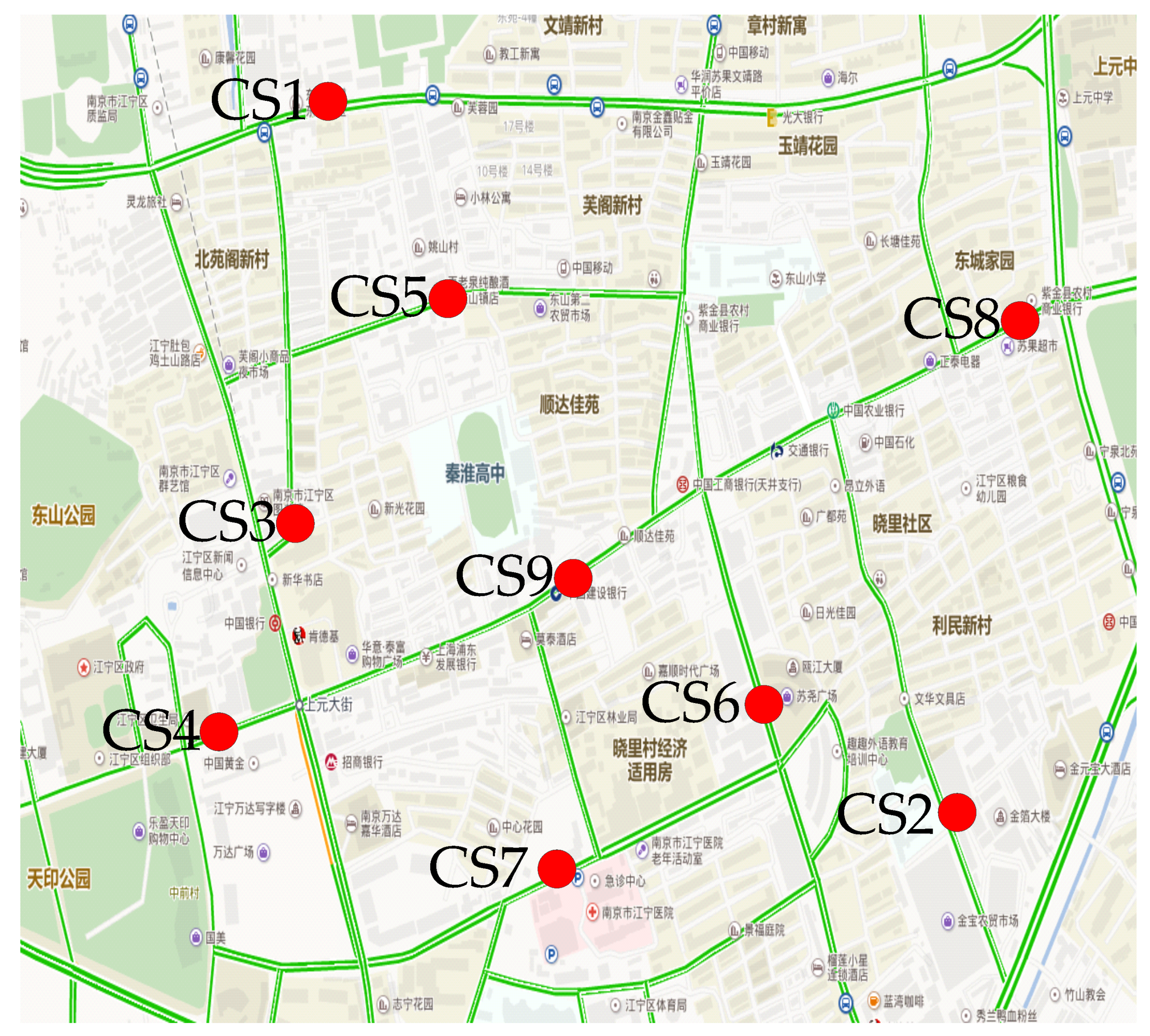
4.1. Simulation Environment

The research selected an experimental area in Nanjing, Jiangsu Province (China) to verify the validity of the proposed high-efficiency charging service system. As shown in Figure 4, the area covers 35 km² and the main road network was applied to establish the road network parameters used in subsequent simulation. The area includes nine EV CSs, among which CSs 1–4 are conventional grid-connected ones, and CSs 5–9 are grid-connected ones containing new energy sources and energy storage. The detailed configuration information pertaining to the CSs is summarized in

Table 2. Configuration parameters of the CSs.

CSID	Capacity of Distribution Transformer/kW	Installed Capacity of New Energies/kW	Energy-Storage Capacity/kW·h	Number of 60 kW Charging Pile	Number of 120 kW Charging Pile
1	400	0	0	4	2
2	400	0	0	6	1
3	240	0	0	5	0
4	240	0	0	5	0
5	250	250	250	5	0
6	250	250	250	5	0
7	400	200	250	5	2
8	400	200	250	5	2
9	800	300	500	10	4

, and the configuration parameters of the EVs for simulation are listed in

Table 3. Configuration parameters of the EVs.

Model	Charging Power/kW	Capacity of Power Battery/kW·h
CarI	60	20
CarII	120	35

. The ratio of CarI to CarII is 2 to 1. The EVs applying for charging appear at random positions on the simulated road network. Assume that the initial SoC of the ESB when the EVs apply for charging meets the condition of N(0.4, 0.1²) [29], and the SoC at the end of charging is 80%. To verify the validity of the algorithm, two different scenarios were selected for simulation analysis of the average waiting time for charging and the immediate utilization rate of new energies in the area: (1) the capacity of the distribution network k is sufficient (Scenario A) and (2) the capacity of the distribution network is constrained (Scenario B). The step size is 1 min throughout the simulation. Moreover, CS9 is selected to verify the effect of the CSEC through simulation.

4.2. Scenario A and Simulation Results

4.2.1. Introduction of Scenario A

In the scenario, the charging of EVs is not constrained by the capacity of the distribution network. To verify the effectiveness of the proposed high-efficiency EV charging service system, other two commonly used EV charging methods were adopted for comparison:

(1)

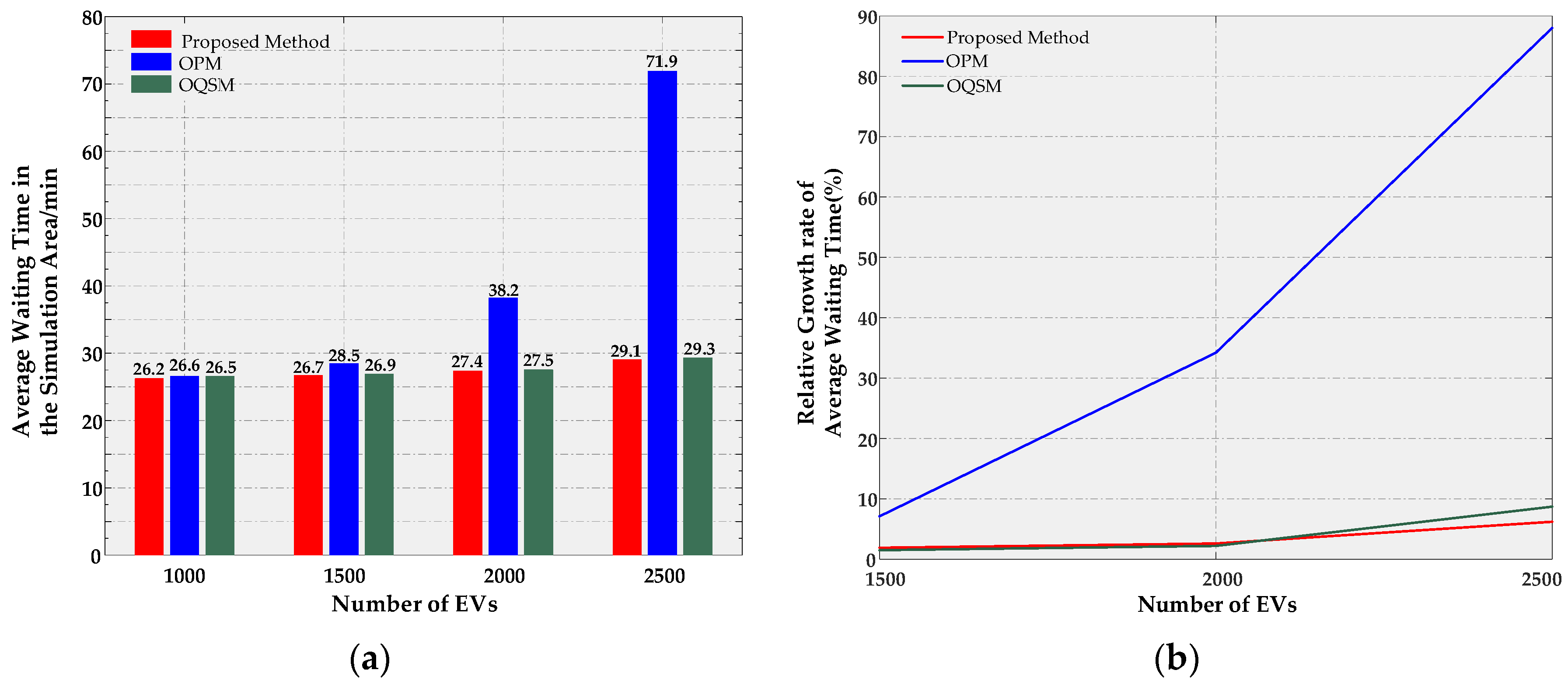
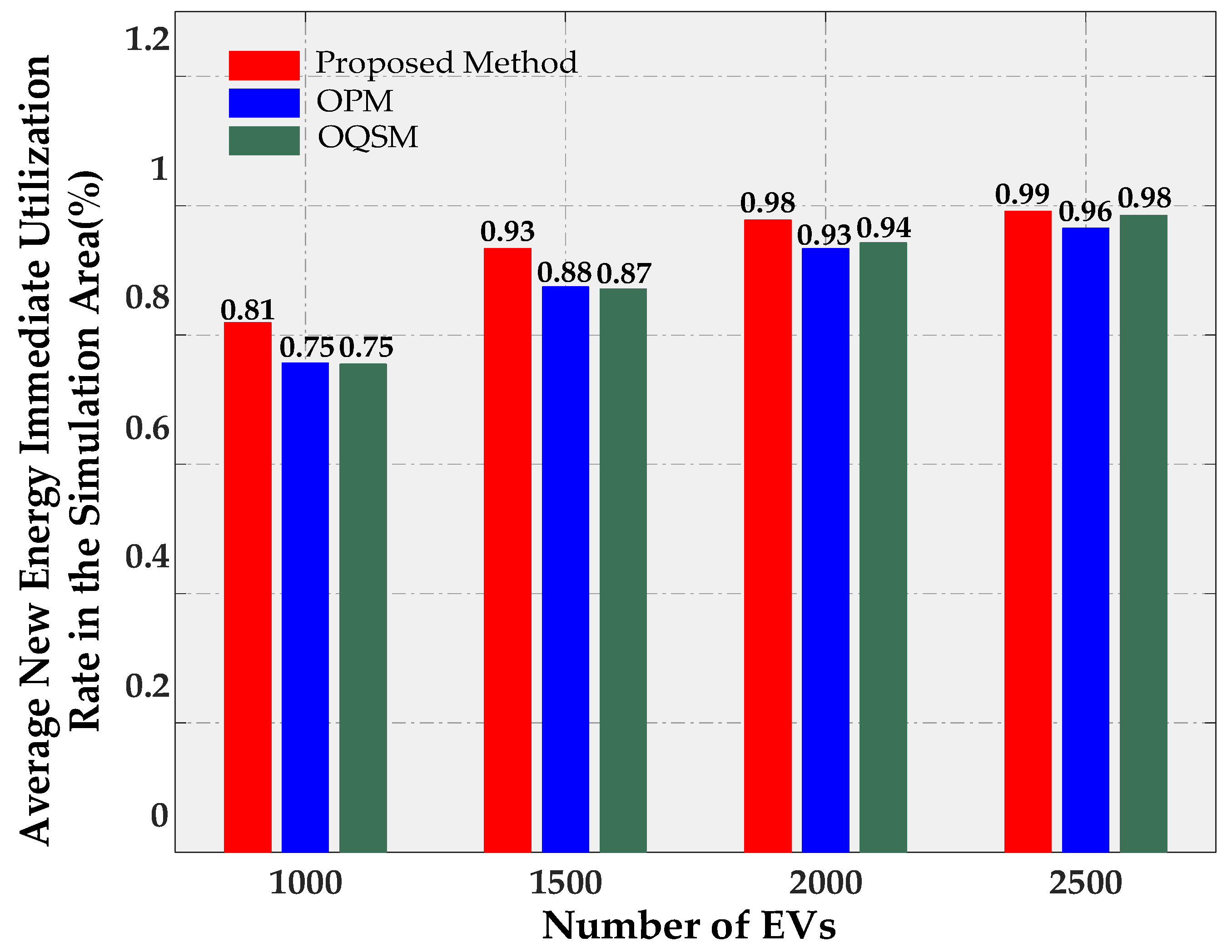
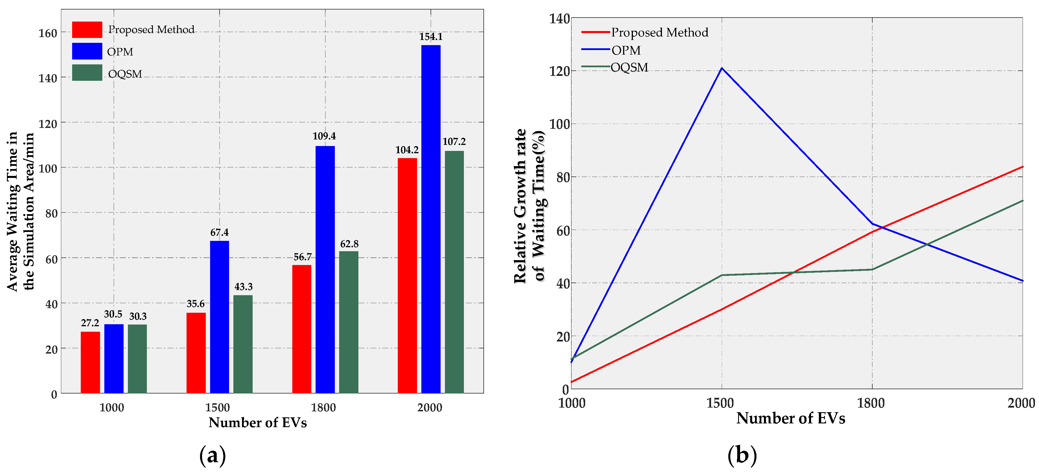
Optimal path method (OPM): the EV owners select a CS in D_i^max with the shortest travel time by comprehensively considering the distance and the travel time to the CSs.

(2)

Optimal queue size method (OQSM): the EV owners select a CS in D_i^max with the smallest queue size by comprehensively considering the distance to the CSs and the queue sizes at each CS.

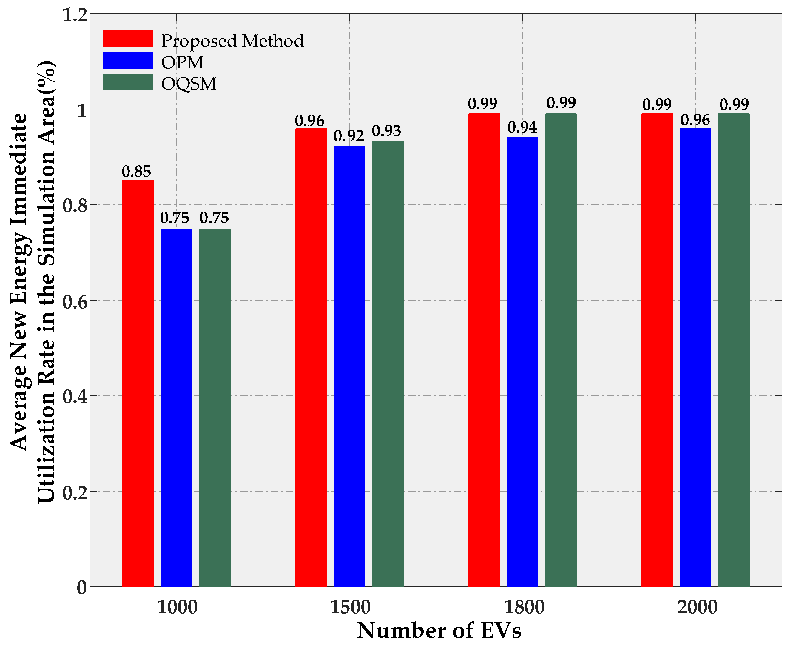
4.2.2. Simulation Results

Figure 5 shows the waiting time of EVs for charging using the three different methods in the simulation area in one day in Scenario A. It can be seen from Figure 5a that the average waiting time for EV charging using the OPM method is longer than that using the other two methods, and it becomes much longer as the number of EVs increases. By using the proposed method and the OQSM method, similar average waiting times are needed for charging, and the average waiting time needed while using the proposed method is slightly shorter than that employing the OQSM method. Figure 5b shows that the relative rate of increase in the average waiting time for charging based on the OPM method is the largest, while that based on the proposed, and OQSM, methods remained lower. Meanwhile, the relative rate of increase of the average waiting time needed when the proposed method is used is slightly lower than that required using the OQSM method. The simulation results of these two aspects of the operation prove that the application of the proposed method is able to reduce the average waiting time for EV charging in the simulation area. Meanwhile, the proposed method also inhibits the increase in average waiting time in the area as the number of EVs is increased.

Figure 6 shows the immediate utilization rates of new energy sources at CSs in the simulation area using the three different methods in Scenario A. The results indicate that charging using the proposed method is able to improve the immediate utilization rate of new energy sources. With an increasing number of EVs, the immediate utilization rate of new energies can approximate to the maximum achieved at a faster speed by charging using the proposed method.

4.3. Scenario B and Simulation Result

4.3.1. Introduction of Scenario B

In Scenario B, the charging of EVs is constrained by the capacity of the distribution network. To verify the effectiveness of the proposed high-efficiency EV charging service system, the NCPM charging method was also used, in addition to the charging methods used in Scenario A. The NCPM method is similar to the proposed method, the only difference being that it does not entail the use of the CS energy control link of the proposed method.

4.3.2. Simulation Results

The curves of the distribution network load for charging in the simulation area using the NCPM and the proposed method in Scenario B are shown in Figure 7. The curves are obtained through superposition of the conventional, and EV, load curves in the area. Some 1000 EVs are involved in the simulation. The simulation results reveal that, while using the NCPM method to charge EVs in the period from 04:00 to 08:00, the obtained distribution network load is higher than the maximum adjustable capacity of the distribution network in the area. When the proposed method is used, the actual load can be maintained at below the maximum adjustable capacity of the distribution network, thus avoiding an overload of the distribution network caused by the charging of EVs.

Figure 8 shows the average waiting time for charging EVs in the simulation area using the three different methods in Scenario B in one day. It can be seen from Figure 8a that the proposed method can more effectively reduce the average waiting time for EV charging compared with the other two methods. As shown in Figure 8b, the proposed method still can inhibit the growth of the average waiting time with the increase in the number of EVs, especially when the number of EVs is between 1000 and 1500; however, as the number of EVs grows beyond 1500, the proposed method is found to have a decreasing inhibitory effect on the growth of the waiting time, especially when there are 1800 to 2000 EVs. Despite this, the average waiting time for charging EVs using the proposed method is still the shortest in comparison with the other two methods.

Figure 9 shows the immediate utilization rates of new energy sources at CSs when EVs are charged using the three different methods in Scenario B. The simulation results are consistent with those in Figure 6, which proves that the proposed method is still feasible even if the capacity of the distribution network is constrained.

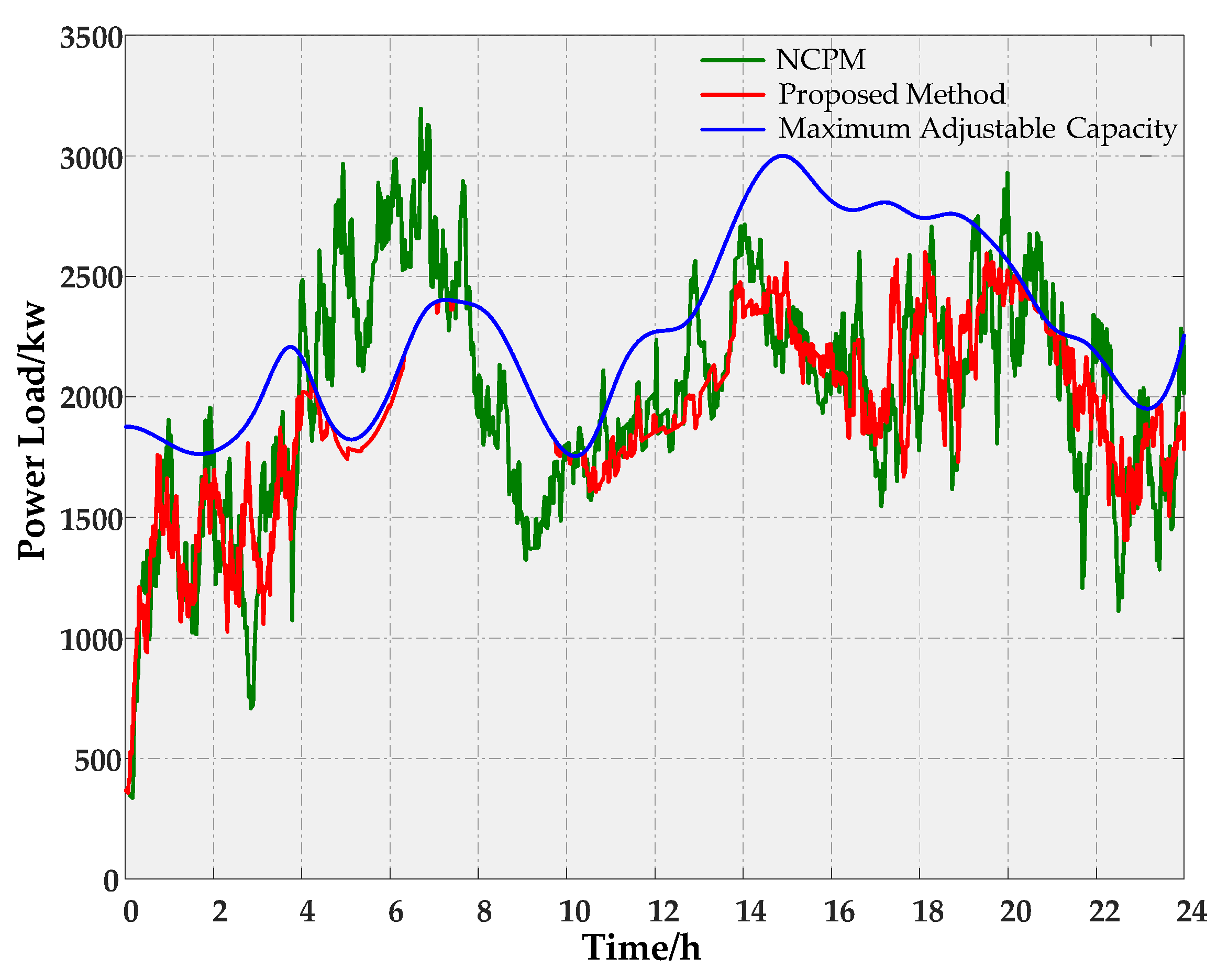
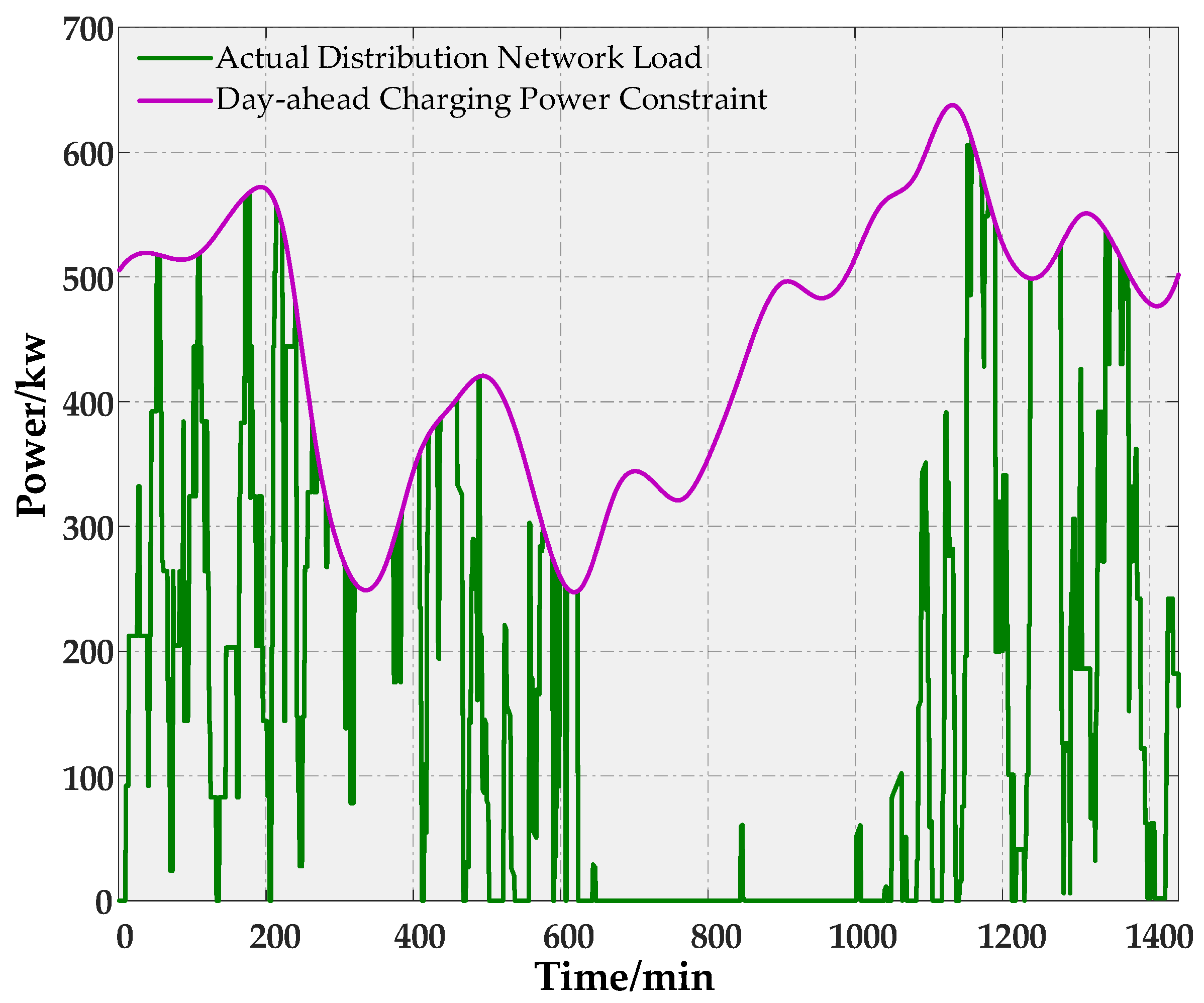
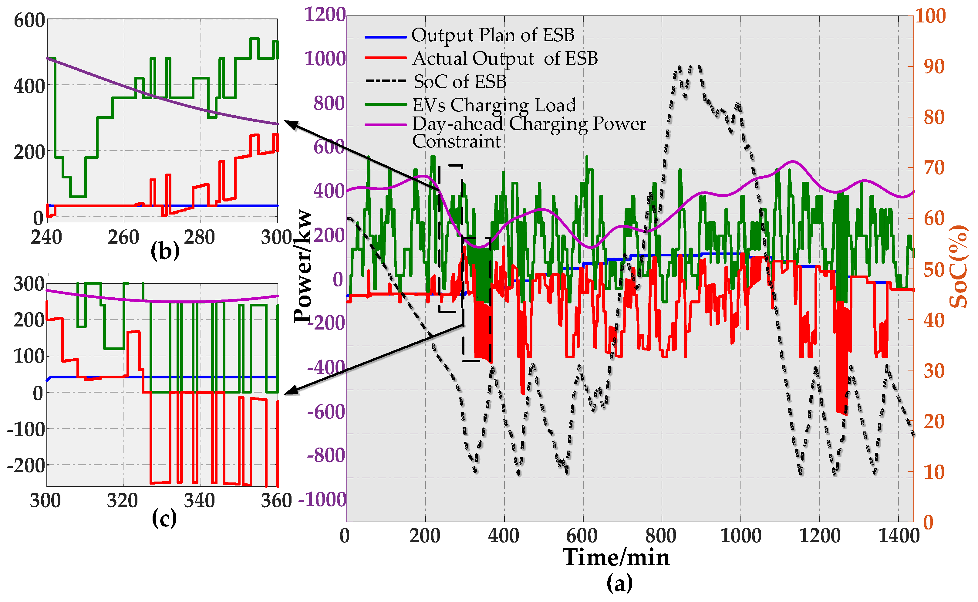
4.4. Simulation of CS Energy Control

CS9 is selected to verify the effect of the CSECA The allowable range of the SoC of the ESB for simulation is 10% to 90%, the MidSoC is 30%, and the control interval Δ is 1 min. Some 1500 EVs are involved in the simulation. Figure 10 shows the simulation results of CS9 using the CSECA algorithm. It can be seen from Figure 10a that the actual charging load of the EVs is higher than the day-ahead charging power constraint in some time periods and the SoC of the ESB is always within the allowable range in a 24 h period. These results indicate that, under the control of the CSEC, CS9 cannot only meet the charging demand of more EVs, but also guarantees that the ESB works in the allowable range of SoC while regulating the ESB. Meanwhile, the ESB is charged after the SoC reaches approximately 10%, and the charging state does not end before the SoC recovers to MidSoC. Figure 10b shows that the CSEC timeously adjusts the output of the ESB to fill the power shortage when the charging load of the EVs exceeds the power constraint of the distribution network, so as to meet the charging demand of EVs as far as possible. As shown in Figure 10c, the CSECA algorithm adjusts the output of the ESB to turn in the charging state when the SoC of the ESB reaches the minimum value of its allowable range, thus protecting the ESB. Moreover, the actual charging power of the ESB is always based on the precondition of maximally meeting the charging demand of the EVs. When the charging demand of EVs is larger than the day-ahead charging power constraint, the ESB also stops charging; when the charging demand of EVs is lower than the day-ahead charging power constraint, the ESB charges the EVs with the difference between the charging demand and the power constraint. The above results prove that the CSECA is able to achieve Algorithm 2.

Figure 11 shows the actual distribution network load and the day-ahead charging power constraint of the CS9 within 24 h under the effect of the CSECA algorithm. It can be seen from the figure that under the control effect of the algorithm, the actual distribution network load is always within the allowable range, thus verifying that the CSECA algorithm is able to realize Algorithm 1.

5. Conclusions

A high-efficiency EV charging service system is proposed with a view to solving problems arising from the increased driving range and the scale development of EVs. The proposed system provides charging reservation and charging pile binding services and is composed of four parts: CDTP, SGOMS, CMP, and CSEC. We also introduce the main communication framework of the system and formulate service rules to guarantee benefit to the CSs. In terms of the spatial guidance of charging, a three-level CS selection model is established for the purposes of shortening the average waiting time for EV charging and improving the immediate utilization rate of new energy sources. We focus on the aims of each level of the CS selection model and relationship between these levels. As to the charging control, the proposed CSECA control algorithm and its control nodes are analyzed. The algorithm has two aims: ensuring the actual distribution network load of CSs is within the day-ahead charging power constraint (Algorithm 1), which is realized using a sub-algorithm (Algorithm 1); and filling the power shortage using an ESB to reduce the influences of the power constraint of the distribution network on the charging of EVs (Algorithm 2), which is achieved by another two sub-algorithms (Algorithms 2 and 3). Finally, an experimental area in Nanjing was selected to verify the proposed model and algorithm through use of a simulation. The simulation results prove the utility of the proposed model and algorithm in shortening the waiting time for EV charging in the simulation area, improving the average immediate utilization rate of new energy sources in the simulation area, and ensuring the distribution network load remains within the allowable range. Verified as effective, the proposed model and algorithm will be applied to a real EV charging project in future research.

References

1. Fan, P.; Sainbayar, B.; Ren, S. Operation Analysis of Fast Charging Stations with Energy Demand Control of Electric Vehicles. IEEE Trans. Smart Grid 2015, 6, 1819–1826. [Google Scholar] [CrossRef]
2. Tan, J.; Wang, L. Real-Time Charging Navigation of Electric Vehicles to Fast Charging Stations: A Hierarchical Game Approach. IEEE Trans. Smart Grid 2015, 2, 846–856. [Google Scholar] [CrossRef]
3. Yunus, K.; Parra, H.Z.D.L.; Reza, M. Distribution grid impact of Plug-In Electric Vehicles charging at fast charging stations using stochastic charging model. In Proceedings of the IEEE European Conference on Power Electronics and Applications, Birmingham, UK, 30 August–1 September 2011; pp. 1–11. [Google Scholar]
4. Yang, S.N.; Cheng, W.S.; Hsu, Y.C.; Gan, C.-H.; Lin, Y.-B. Charge Scheduling of Electric Vehicles in Highways through Mobile Computing. Math. Comput. Model. 2013, 57, 2873–2882. [Google Scholar] [CrossRef]
5. Gusrialdi, A.; Qu, Z.; Simaan, M.A. Scheduling and cooperative control of electric vehicles’ charging at highway service stations. In Proceedings of the IEEE 53rd Annual Conference on Decision and Control (CDC), Los Angeles, CA, USA, 15–17 December 2014; pp. 6465–6471. [Google Scholar]
6. Razo, V.D.; Jacobsen, H.A. Smart Charging Schedules for Highway Travel with Electric Vehicles. IEEE Trans. Transp. Electr. 2016, 2, 160–173. [Google Scholar] [CrossRef]
7. Gusrialdi, A.; Qu, Z.; Simaan, M.A. Distributed Scheduling and Cooperative Control for Charging of Electric Vehicles at Highway Service Stations. IEEE Trans. Intell. Transp. Syst. 2017, 18, 2713–2727. [Google Scholar] [CrossRef]
8. Brenna, M.; Longo, M.; Yaïci, W. Modelling and Simulation of Electric Vehicle Fast Charging Stations Driven by High Speed Railway Systems. Energies 2017, 10, 1268. [Google Scholar] [CrossRef]
9. Rigas, E.S.; Ramchurn, S.D.; Bassiliades, N.; Koutitas, G. Congestion management for urban EV charging systems. In Proceedings of the IEEE International Conference on Smart Grid Communications (SmartGridComm), Vancouver, BC, Canada, 21–24 October 2013; pp. 121–126. [Google Scholar]
10. Schürmann, D.; Timpner, J.; Wolf, L. Cooperative Charging in Residential Areas. IEEE Trans. Intell. Transp. Syst. 2017, 99, 1–13. [Google Scholar] [CrossRef]
11. Szczurek, P.; Xu, B.; Wolfson, O.; Lin, J.; Rishe, N. Learning the relevance of parking information in VANETs. In Proceedings of the Seventh ACM International Workshop on VehiculAr Internetworking, Chicago, IL, USA, 24 September 2010; ACM: New York, NY, USA, 2010; pp. 81–82. [Google Scholar]
12. Cao, Y.; Kaiwartya, O.; Wang, R.; Jiang, T.; Cao, Y.; Aslam, N.; Sexton, G. Toward Efficient, Scalable, and Coordinated on-the-Move EV Charging Management. IEEE Wirel. Commun. 2017, 24, 66–73. [Google Scholar] [CrossRef]
13. Silvestre, D.; Sanseverino, R.; Zizzo, G.; Graditi, G. An optimization approach for efficient management of EV parking lots with batteries recharging facilities. J. Ambient Intell. Humaniz. Comput. 2013, 4, 641–649. [Google Scholar] [CrossRef]
14. Clement-Nyns, K.; Haesen, E.; Driesen, J. The Impact of Charging Plug-In Hybrid Electric Vehicles on a Residential Distribution Grid. IEEE Trans. Power Syst. 2010, 25, 371–380. [Google Scholar] [CrossRef] [Green Version]
15. Mu, Y.; Wu, J.; Jenkins, N.; Jia, H.; Wang, C. A Spatial–Temporal model for grid impact analysis of plug-in electric vehicles. Appl. Energy 2014, 114, 456–465. [Google Scholar] [CrossRef]
16. Qian, K.; Zhou, C.; Allan, M.; Yuan, Y. Modeling of Load Demand Due to EV Battery Charging in Distribution Systems. IEEE Trans. Power Syst. 2011, 26, 802–810. [Google Scholar] [CrossRef]
17. Awadallah, M.A.; Singh, B.N.; Venkatesh, B. Impact of EV Charger Load on Distribution Network Capacity: A Case Study in Toronto. Can. J. Electr. Comput. Eng. 2016, 39, 268–273. [Google Scholar] [CrossRef]
18. Wang, Z.; Wang, S. Grid Power Peak Shaving and Valley Filling Using Vehicle-to-Grid Systems. IEEE Trans. Power Deliv. 2013, 28, 1822–1829. [Google Scholar] [CrossRef]
19. Xi, X.; Sioshansi, R. Using Price-Based Signals to Control Plug-in Electric Vehicle Fleet Charging. IEEE Trans. Smart Grid 2014, 5, 1451–1464. [Google Scholar] [CrossRef]
20. Hu, Z.; Zhan, K.; Zhang, H.; Song, Y. Pricing mechanisms design for guiding electric vehicle charging to fill load valley. Appl. Energy 2016, 178, 155–163. [Google Scholar] [CrossRef]
21. Ghavami, A.; Kar, K.; Bhattacharya, S.; Gupta, A. Price-driven charging of Plug-in Electric Vehicles: Nash equilibrium, social optimality and best-response convergence. In Proceedings of the 47th Annual Conference on Information Sciences and Systems (CISS), Baltimore, MD, USA, 20–22 March 2013; pp. 1–6. [Google Scholar]
22. Luo, C.; Huang, Y.F.; Gupta, V. Stochastic Dynamic Pricing for EV Charging Stations with Renewables Integration and Energy Storage. IEEE Trans. Smart Grid 2018, 9, 1494–1505. [Google Scholar] [CrossRef]
23. Fan, H.; Hou, H.; Ke, X.; Zhu, G.; Chen, W. The Optimal Charging Strategy of EV Rational User Based on TOU Power Price. In Proceedings of the IEEE International Conference on Industrial Informatics—Computing Technology, Intelligent Technology, Industrial Information Integration, Wuhan, China, 3–4 December 2016; pp. 376–379. [Google Scholar]
24. Liu, M.; Mcloone, S.; Studli, S.; Middleton, R.; Shorten, R.; Braslavs, J. On-off based charging strategies for EVs connected to a Low Voltage distributon network. In Proceedings of the IEEE PES Asia-Pacific Power and Energy Engineering Conference (APPEEC), Kowloon, China, 8–11 December 2013; pp. 1–6. [Google Scholar]
25. Masuch, N.; Keiser, J.; Lützenberger, M.; Albayrak, S. Wind power-aware vehicle-to-grid algorithms for sustainable EV energy management systems. In Proceedings of the IEEE International Electric Vehicle Conference (IEVC), Greenville, SC, USA, 4–8 March 2012; pp. 1–7. [Google Scholar]
26. Zheng, J.; Wang, X.; Men, K.; Zhu, C.; Zhu, S. Aggregation Model-Based Optimization for Electric Vehicle Charging Strategy. IEEE Trans. Smart Grid 2013, 4, 1058–1066. [Google Scholar] [CrossRef]
27. Yagcitekin, B.; Uzunoglu, M. A double-layer smart charging strategy of electric vehicles taking routing and charge scheduling into account. Appl. Energy 2016, 167, 407–419. [Google Scholar] [CrossRef]
28. Chaudhari, K.; Ukil, A.; Kumar, K.N.; Manandhar, U.; Kollimalla, S.K. Hybrid Optimization for Economic Deployment of ESS in PV Integrated EV Charging Station. IEEE Trans. Ind. Inf. 2017, 14, 101–116. [Google Scholar] [CrossRef]
29. Xu, Z.; Su, W.; Hu, Z.; Song, Y.; Zhang, H. A Hierarchical Framework for Coordinated Charging of Plug-In Electric Vehicles in China. IEEE Trans. Smart Grid 2017, 7, 428–438. [Google Scholar] [CrossRef]
Figure 1. Framework of the high-efficiency electric vehicles (EVs) charging service system.
Energies 11 00911 g001
Figure 2. The communication framework of the sub-systems in the high-efficiency EV charging service system.
Energies 11 00911 g002
Figure 3. The CSECA procedure and its control diagram.
Energies 11 00911 g003
Figure 4. Map of the simulation area.
Energies 11 00911 g004
Figure 5. Simulation results under conditions in which three different charging methods are used. (a) Average waiting time in the simulation area; (b) Relative rate of growth of average waiting time.
Energies 11 00911 g005
Figure 6. Average immediate utilization rates of new energy sources in the simulation area when the three different methods are used for charging.
Energies 11 00911 g006
Figure 7. Curves of the distribution network load in the simulation area when the NCPM and the proposed method are used.
Energies 11 00911 g007
Figure 8. Simulation results while charging using the three different methods. (a) Average waiting time in the simulation area; (b) Relative growth rate in average waiting time.
Energies 11 00911 g008
Figure 9. Average immediate utilization rates of new energy sources in the simulation area when the three different charging methods are used.
Energies 11 00911 g009
Figure 10. Simulation results for CS9 under the effect of the CESCA. (a) Curves of the output plan of the ESB, actual output of the ESB, SoC of the ESB, charging load of EVs, and day-ahead charging power constraint; (b) Partially enlarged view on the interval [240, 300]; (c) Partially enlarged view on the interval [300, 360].
Energies 11 00911 g010
Figure 11. Curves of actual distribution network load and the day-ahead charging power constraint under the effect of the CSECA.
Energies 11 00911 g011