Force Analysis of a Circular Cylinder at Ununiformed Flow in a T Pipe Junction


1
Key Laboratory of Thermo-Fluid Science and Engineering, Ministry of Education, School of Energy and Power Engineering, Xi’an Jiaotong University, Xi’an 710049, China
2
Department of Mechanical Engineering, Lanzhou Jiaotong University, Lanzhou 730070, China
*
Author to whom correspondence should be addressed.
Energies 2018, 11(4), 864; https://doi.org/10.3390/en11040864
Submission received: 1 March 2018
/
Revised: 4 April 2018
/
Accepted: 6 April 2018
/
Published: 8 April 2018
(This article belongs to the Section I: Energy Fundamentals and Conversion)
Abstract
:Experimental and numerical investigations of force analysis acted on single circular cylinder in the T pipe junction with the effect of vanes are reported in this paper. Experiments are carried on in a small wind tunnel at five different velocity ratios (R) from 0.117 to 0.614. The mean pressure data acted on the cylinder are obtained and in turn the drag and lift. Vanes are installed at the junction to change the secondary flow in the suction duct and the angle is in the range of 90° ≤ φ ≤ 130°. Numerical studies which are validated by the experimental data help understand the flow structure for the analysis. It is found that in the T shape junction without vanes, the cylinder presents different surface mean pressure distributions at the different positions in the suction duct. As the increase of the distance from the junction to the cylinder center, the surface mean pressure distributions recover to the benchmark gradually which performs in the straight duct beforehand. Four feature points including the front/rear stagnation points and the separation points and the corresponding three divisions of flow region are analyzed in detail with the auxiliary numerical simulation of flow structure. Effect of the vanes with different angle is also discussed. Finally, the drag and lift coefficients acted on the cylinder with or without vanes are performed.
1. Introduction
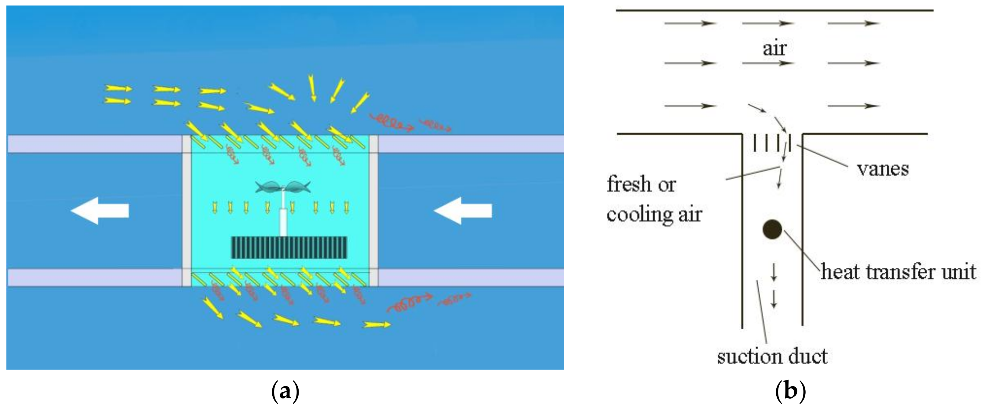
Recent years have seen many great changes taking place in China’s transportation, especially in high speed railways which mileage has increased to more than 25 thousand kilometers in five years, representing 2/3 of the world totally. Ventilation and heat transfer are the main aerodynamic problems when trains are running in underground stations and tunnels as they can affect the trains’ thermal comfort, efficiency, stability, safety and other characteristics together with the comfort for passengers and prevention of disasters [1]. For the experimental study, the practical ventilation and heat transfer units of the high speed shear flow can be simplified as a wind tunnel model as depicted in Figure 1. Through the vanes impeding entry of external trash at the ventilation ports, fresh or cooling air flows into the suction duct and then forces convection with the heat transfer unit by the action of a draught fan, so the flow at the ventilation parts can be simplified as flow past a single circular cylinder in the branch of a T pipe junction.
Flow past a circular cylinder has recently received a number of experimental [2,3] and computational [4,5] investigations due to its typical complicated turbulent characteristic and extensive engineering application over the past decades. The main flow features include the pressure coefficient, drag/lift, skin friction, separation angle and also Strouhal number, which are highly Reynolds number (Re) relevant, together with the geometrical effects such as the aspect ratio and blockage [6,7]. Divided by the Re in engineering, the turbulent flow past a cylinder exhibits several regions as defined [2,8,9]: sub-critical for 3 × 10² < Re < 2 × 10⁵, critical for 2 × 10⁵ < Re < 3.5 × 10⁵, supercritical for 3.5 × 10⁵ < Re < 1.5 × 10⁶ and post-critical for Re > 1.5 × 10⁶.
In experimental studies, West and Apelt [10] examined the effect of aspect ratio and blockage ratio on pressure distribution, drag coefficient, Strouhal number and the spanwise cross-correlations of fluctuating pressures. They found that for blockage ratios in the range 6–l6%, reduction in aspect ratio had effects on drag coefficient and on base pressure coefficient which were similar to those associated with increase in blockage ratio and the blockage correction procedures based on the image method and the momentum method [11,12] were unsatisfactory in their prediction of the unblocked drag coefficient but the momentum method predicted the unblocked base pressure coefficient quite well. Cantwell and Coles [13] conducted an experimental study of entrainment and transport in the turbulent near wake of a circular cylinder.
They reached an important conclusion that a substantial part of the turbulence production is concentrated near the saddles and that the mechanism of turbulence production is probably vortex stretching at intermediate scales. Another two dimensional parameters-Strouhal number and mean base suction coefficient affected by the aspect ratio were investigated by Norberg [14]. It was found that different aspect ratios are needed for the independent condition at higher Re. Tsutsui and Igarashi [15] reported a method to reduce the drag in air-stream by using a rod in front of the cylinder. An optimum condition was obtained that vortices do not shed from the rod and the shear layer from the rod reattaches on the front face of the circular cylinder. The total drag with the rod is 63% less than the standard single cylinder. Bearman [16] presented the vortex shedding around single cylinder at the critical Re. The cylinder can be treated as two-dimensional with the organized vertex shedding when the Re is less than 5.5 × 10⁵. The Strouhal number reaches a maximum value of 0.46 when the mean drag coefficient is a minimum. The local pressure and skin friction around a circular cylinder at post critical Re region were exhibited by Achenbach [17]. Three flow states are defined according to the position of the separation points, separation bubbles or transition points acquired by calculating the skin friction distribution. Shih et al. [18] investigated the rough cylinder in the crossflow at with Re up to 8 × 10⁶. The difference between steady and unsteady with the roughness and the drag coefficient independent area for Re were obtained.
The circular cylinder flow has also attracted lots of attention in numerical simulations, including the steady and unsteady by means of the Reynolds average Naiver-Stokes (RANS) models or the scale-resolving simulation (SRS) models. Breuer [19] mainly studied the numerical and modeling influence on the large eddy simulation (LES) of flow past cylinder. Most important advices were achieved such as the better central schemes of second- or fourth-order accuracy in space. Different subgrid scale modeling and spanwise resolution have also been studied. Kravchenko and Moin [20] reported a new space discretize method based on the B-splines for the investigation of flow over a circular cylinder at ReD = 3900. Better agreement with the experimental measurements were obtained farther downstream the cylinder, especially the power spectra of fluctuating velocity. A comparison of near weak of a cylinder by using four classic turbulent models was conducted by Ünal et al. [21]. From the report the Shear-Stress-Transport k-(SST k-) model is the best RANS choose for the flow which has the adverse pressure gradient and vortex shedding. Yeon et al. [22] presented a systematic LES study on the flow over the circular cylinder in a large range of Re. They found that large aspect ratio is needed at sub-critical Re while small aspect ratio appears important at critical and super-critical Re. The turbulence separation is the most difficult to predict. Drag crisis was captured by Lloyd and James [23] by using the different grid size and numerical strategy. The Re is in the range of 6.31 × 10⁴ to 5.06 × 10⁵. It was shown that the dynamic subgrid model is better than the conventional Smagorinsky model and the discretization of the convection scheme plays an important role when adopting the coarse grid. Catalano et al. [24] presented LES and RANS simulations around the circular cylinder at the supercritical region. It was found that the LES model is more accurate than the RANS model, but the Re dependence is not captured. Ong et al. [25] employed two-dimensional unsteady RANS equations with a standard high Reynolds number k- turbulence model to simulate the flow past a circular cylinder in the post-critical region. It was shown that the model has good applicability in engineering design.
The oncoming flow past the circular cylinder of the previously mentioned literatures are mainly uniform flow, while few researchers have studied the non-uniform condition, such as the suction flow in the T pipe junction with the intense secondary flow. In the present paper, experimental investigations of force analysis acted on single circular cylinder in the T pipe junction with the effect of vanes in wind tunnel are reported at the five velocity ratios (R) from 0.117 to 0.614 and the twelve positions in the suction duct. In the following parts, Section 2 and Section 3 systematically introduce the experimental system and the corresponding analyses in detail. A benchmark test is firstly carried out to validate the experimental method, also compared with the following measurements in a T pipe junction. Section 4 describes the numerical simulation for visualizing the flow structure around the circular cylinder in suction duct. The results and discussion are reported in Section 5, mainly including the pressure coefficient, the drag coefficient and the lift coefficient with and without vanes. Conclusions are summarized in Section 6.
2. Experimental Test Facility and Procedure
2.1. Wind Tunnel
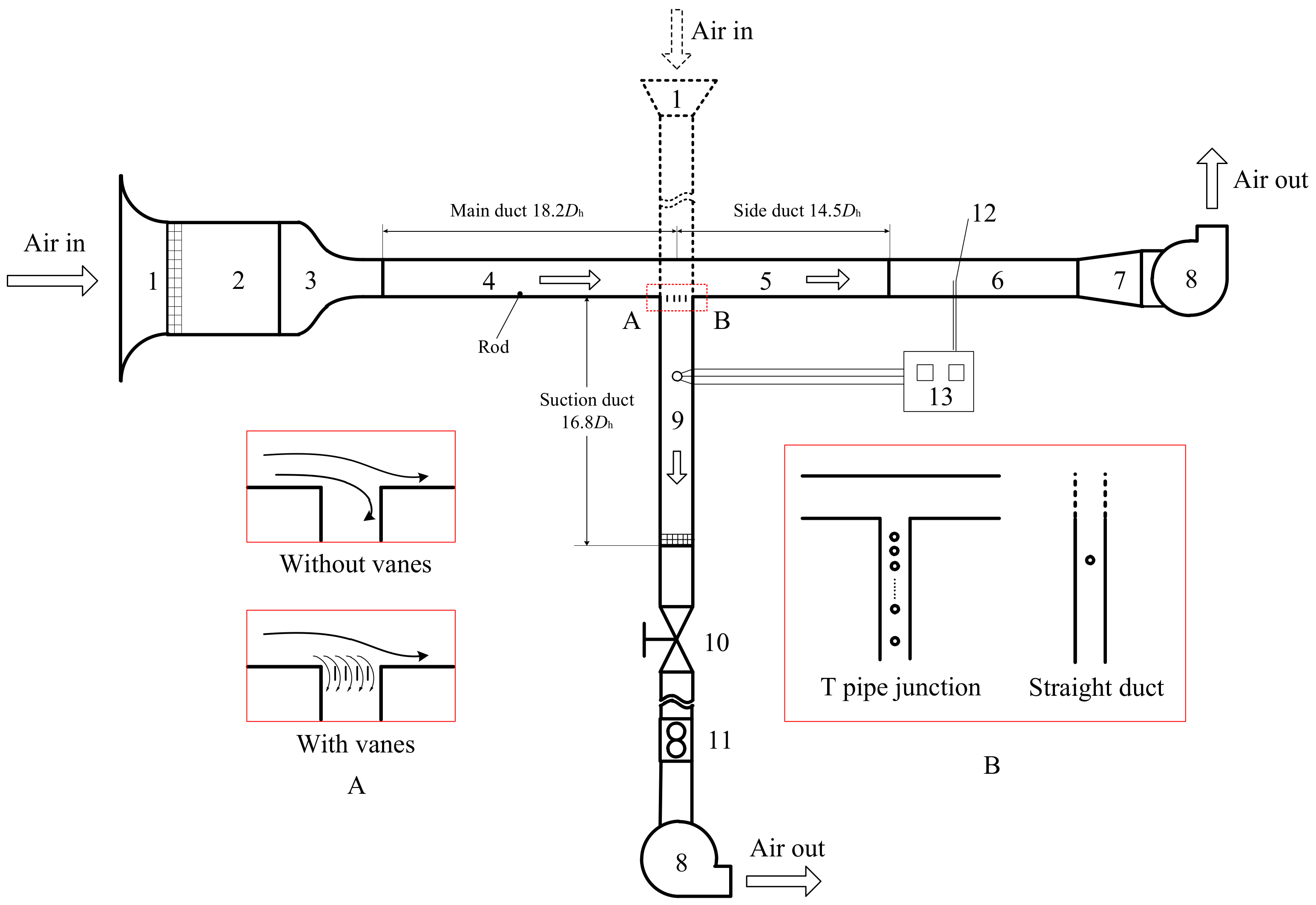
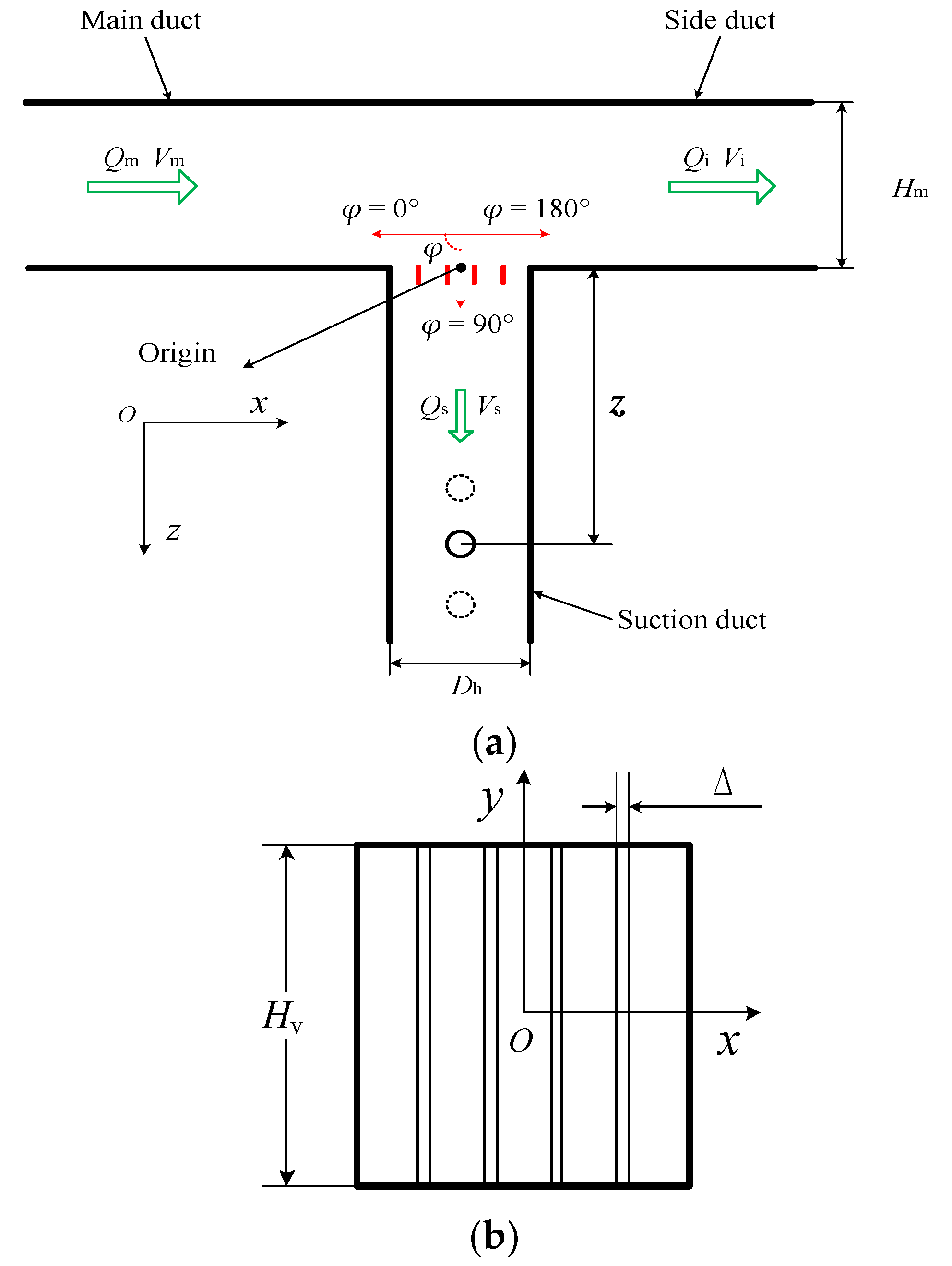
The experimental tests are conducted in a T shape wind tunnel with two variable frequency blowers running at the same time. Three major ducts are included in present system—the main duct, the side duct and the suction duct—as depicted in Figure 2. In the main duct, grid structure and filter screen are mounted between the horn shape entrance and the transition section, which is followed by a 9:1 area contraction section. An iron rod of 2 mm diameter is installed inside the duct wall, 1000 mm away from the main duct inlet, to make the inlet turbulent flow fully developed. Both the main duct and the side duct have the same cross-section of height (Hm) × width (Am) × length (Lm) = 143.3 mm × 161.7 mm × 2000 mm and they are partitioned by the perpendicularly installed square suction duct with the cross-section of 110 mm × 110 mm. Part A in Figure 2 is the local enlarged main duct and suction duct interface with/without vanes in the lower left corner of Figure 2. Part B in Figure 2 is the two kinds of the flow paths, including the flow in the T pipe junction duct and the straight duct in the right lower corner of Figure 2. Four vanes which are made of iron are uniformly mounted at the suction entrance and the angle definition is shown in Figure 3. Each of vanes has x × y × z = 2 mm × 110 mm × 21 mm. The origin of the coordinates is at the suction duct inlet center as shown in Figure 3a. The circular cylinder can move at twelve positions in the suction centerline, z/Dh = 0.5, 1, 1.5, 2, 3, 4, 5, 6, 7, 9, 11, 13. Here z represents the distance between the cylinder and the origin. Dh is the suction duct hydraulic diameter. For the validation of the experimental measurement and the comparison with in the T pipe junction, a benchmark test in an extended suction duct (straight duct) without vanes is carried out beforehand as show in dotted line in Figure 2.
The volume flow rate through the side duct is measured by Pitot tube that connects with an intelligent pressure scanner (PSI) with a precision of 0.1%. The volume flow rate through the suction duct is measured by a rotameter with a precision of 1.5%.
2.2. Test Circular Cylinder
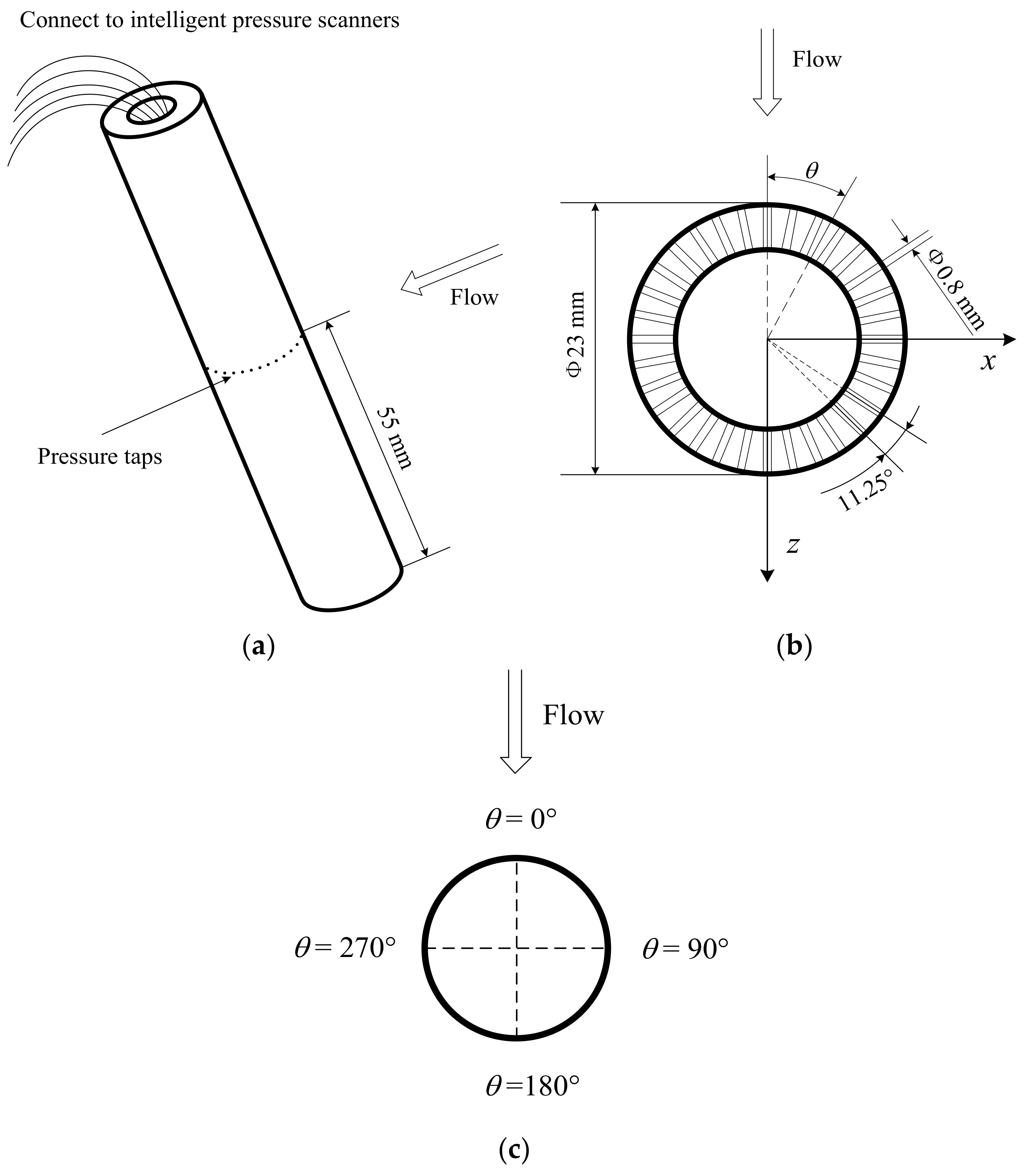
Figure 4 depicts a schematic view of the test cylinder and the angle around the cylinder surface. The outer diameter (d) is 23 mm and the length (l) is 160 mm. It is vertically located at the suction centerline. The material is acrylic glass with smooth surface. There are 32 pressure taps uniformly arrangement around the cylinder surface, as shown in Figure 4a,b. The diameter of the taps is 0.8 mm and suitable capillaries are inserted. Silicon tubes are employed to connect the capillaries and the PSI so the circumferential surface pressure data can be acquired at the same time.
3. Analyses of the Experiment
3.1. Measurement in T Pipe Junction
During the process of all experimental tests in T pipe junction, the suction volume flow rate Qs is fixed at 0.0639 m3/s. The corresponding bulk velocity Vs is 5.28 m/s. The suction bulk velocity Vs is calculated as:
where Ss is the cross-section area of suction duct. Analogously, the corresponding bulk velocities in main duct Vm, and side duct Vi are defined by:
where Sm is the cross-section area of main duct and the side duct. Qm and Qi are the main duct and side duct volume flow rate respectively. Due to the incompressible propriety of air under the test condition, here the main volume flow rate Qm is defined by:
One important dimensionless parameter named velocity ratio R is defined as:
By regulating the frequency of the blowers, five different velocity ratios can be achieved: R = 0.117, 0.150, 0.263, 0.439, and 0.614.
3.2. Measurement in the Straight Duct
One single benchmark experimental test in the extended suction duct (straight duct) is conducted. The volume flow rate keeps the same with that in the suction duct of the T pipe junction as mentioned before, Qs = 0.0639 m3/s. This test can both validate the accuracy of experimental method and compare with the measurements in T pipe junction.
Based on the suction duct bulk velocity Vs and hydraulic diameter Dh, the Reynolds number in the straight duct is Res = 3.6 × 10⁴. It is noticed that in the calculation of Reynolds number for flow past the circular cylinder, the characteristic velocity ought to be the centerline velocity, Vsc. According to Melling and Whitelaw [26], the relationship between Vsc and Vs is given as:
where varies as a function of Res. It is 1.24 based on experimental measurements [26] when the Reynolds number approaches Res = 3.6 × 10⁴. According to the centerline velocity Vsc and the outer diameter of the circular cylinder d, the Reynolds number of flow over the circular cylinder in the straight duct is Rec = 9163.
3.3. Data Processing
Pressure coefficient calculated in the present investigation is a slightly different with the traditional definition which is based on the freestream static pressure and the centerline velocity. Nevertheless, the freestream static pressure does not exist in the T shape model because the inlet flow into the suction duct is not uniform. Therefore the revised pressure coefficient can be calculated as follows:
where Cp (θ) and p(θ) represent the pressure coefficient and the surface pressure at θ degree around the circular cylinder as depicted in Figure 4. Here Vsc is the same value with that in Equation (6) though it does not refer to the freestream centerline velocity in the suction duct of T shape configuration. ρ is the air density and Pmin represents the minimum value of the thirty-two circumference pressure values around the cylinder in experimental test.
The correlation function F(δ) is defined to check the correlation or the similarity between two functions. Here both the pressure distribution curves in straight duct (benchmark) and in T pipe junction are treated as discrete periodic functions. The period is 360 degrees. Then the relevant coefficient σ among them is calculated by:
Another parameter, amplitude ratio AR is defined to exhibit the relative size of maximum values of the surface pressure coefficient between the T pipe junction and the benchmark. It is calculated by:
where and represent the maximum pressure coefficient around the circular cylinder achieved in T pipe junction and in the benchmark, respectively.
Two force analysis parameters including drag coefficient (CD) and lift coefficient (CL) are defined as:
where fz and fx refer to the resultant force on the unit length of circular cylinder in z-direction and x-direction as shown in Figure 3a and r is the radius of the circular cylinder.
3.4. Experimental Uncertainty Analysis
In the present experimental system, the primary obtained parameter is the surface pressure coefficient which is calculated by the pressure and velocity measurements. As mentioned in Section 2.1, both the pressure and the side duct volume flow rate data are acquired by PSI with precisions of 0.1%. The volume flow rate through the suction duct is revealed by a rotameter with a precision of 1.5%. The errors in measuring the cross-section area of the main duct and the suction duct are ±0.001 m2 and ±0.002 m2, respectively. The environmental temperature and barometric pressure are acquired by the experimental facilities with the precisions of ±0.2 °C and 0.03%, respectively. Based on the method described in [27], the maximum uncertainties in calculating pressure and velocity are 0.03% and 4.23% and the primary obtained pressure coefficient has a maximum uncertainty of 6.63%.
3.5. Validation of the Experimental Measurement Method in Straight Duct
3.5.1. Classical Pressure Distribution around Single Circular Cylinder
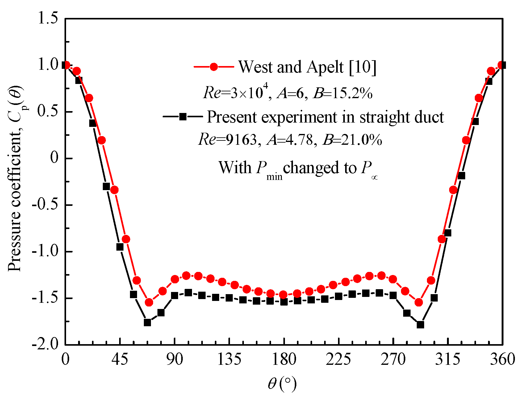
Before the T pipe junction measurements, one benchmark test is conducted in the straight duct under the approximate conditions of West and Apelt [10]. A little difference should be mentioned in calculating the traditional pressure coefficient in straight duct as long as transform Pmin in Equation (7) into the freestream static pressure, P∞. P∞ is defined as follows:
where P(0) is the 0° degree surface pressure as depicted in Figure 4.
Figure 5 shows the comparison between the present benchmark test and the literature data from West and Apelt [10]. Good agreement can be obtained in the variation tendency especially the positions of stagnation and separation points. The measurements in the present case are a bit little than that in West and Apelt [10] which is under the test condition of Re = 3.0 × 10⁴, aspect ratio A = 6 and blockage ratio B = 15.2%. Base on the studies of Norberg and Sunden [28] and Ahmed and Talama [29], the effect of Reynolds number ranging from 104 to 105 can be neglected and the Reynolds number in the present straight duct experimental test is 9163, which is very close to this range, and also both decreases in the aspect ratio and increases in the blockage ratio can lower the pressure coefficient [10].
3.5.2. Drag Coefficient (CD)
Table 1 depicts the comparison of drag coefficient on single circular cylinder in straight duct between present result and the previous study. According to the figures and data in West and Apelt [10], as the Reynolds number is in the range of about 5000 < Re < 50,000, the drag coefficient is influenced by Reynolds number, blockage, and aspect ratio together. Reduction in aspect ratio has effects on drag coefficient and on base-pressure coefficient which is similar to those associated with increase in blockage ratio. Comparing these three sets of data we can find that the blockage and aspect ratio are generally close, so the effect of the Reynolds number governs principally. On the base of the results in West and Apelt [10], the drag coefficient increases with the increase of Reynolds number, the same changing trend as the present result. Meanwhile, the lift coefficient is 0.0018 which can be neglected in the x-direction.
Based on the pressure coefficient and drag coefficient validations, the experimental measurement method can be considered reliable.
4. Numerical Method
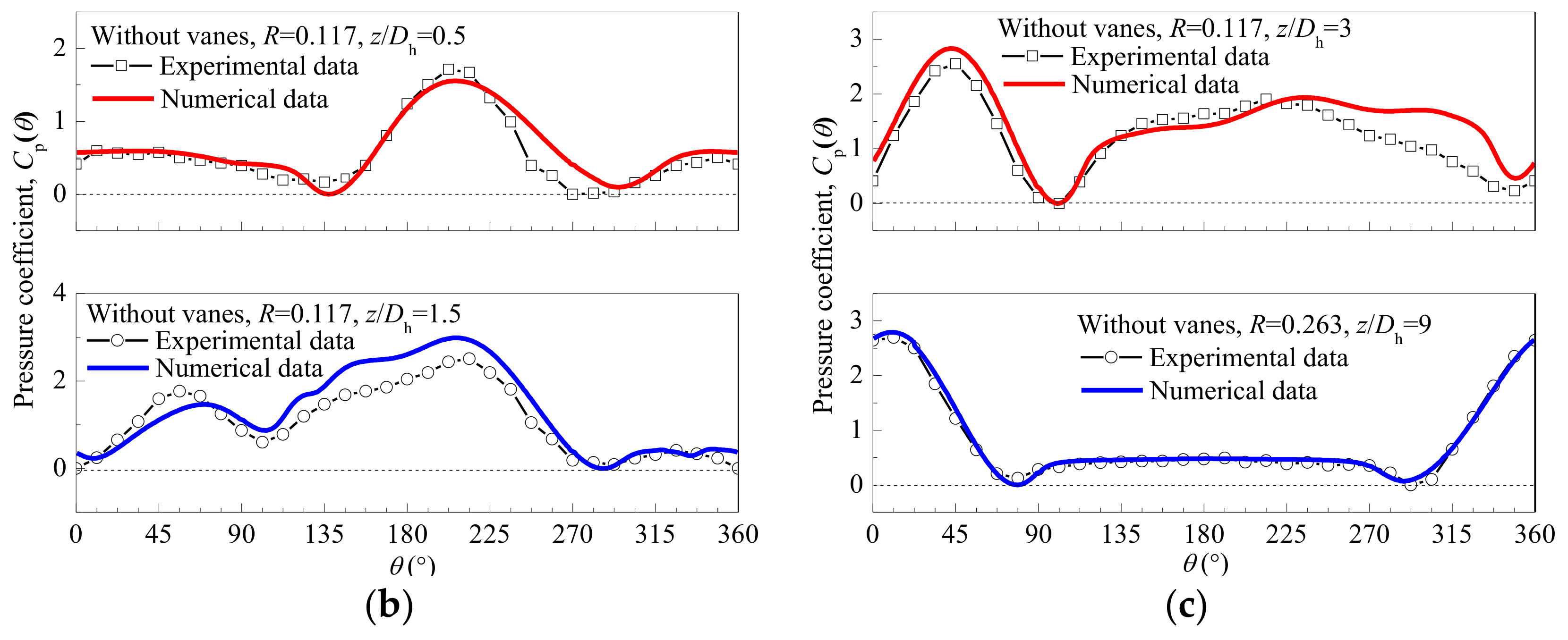
A three-dimensional computational fluid dynamic (CFD) simulation for typical experimental cases is performed by using ASNSY FLUENT 14.5 to obtain the flow characteristics for the analysis of the surface mean pressure distributions. The main calculation model in CFD study is with a proportion of 1:1 with the experimental test section and both the inlet and the two outlets are extended as depicted in Figure 6. Shear-stress transport k- (SST k-) model is selected to model the turbulent due to the better prediction for flow separation and adverse pressure gradient. Detail settings in the calculation are shown in Table 2. Figure 7 depicts the comparisons between CFD results with experimental measurements in T pipe junction with/without vanes. It can be observed that the CFD results in T pipe junction with vanes appear to show good agreement with the experimental data as shown in Figure 7a. CFD and experimental results also show good agreement for T pipe junction without vanes except for a little higher at a few points as depicted in Figure 7b,c. Generally, the calculated CFD results show good agreement with the experimental tests, so the present CFD method is acceptable.
5. Results and Discussion
5.1. Mean Pressure Distribution without Vanes
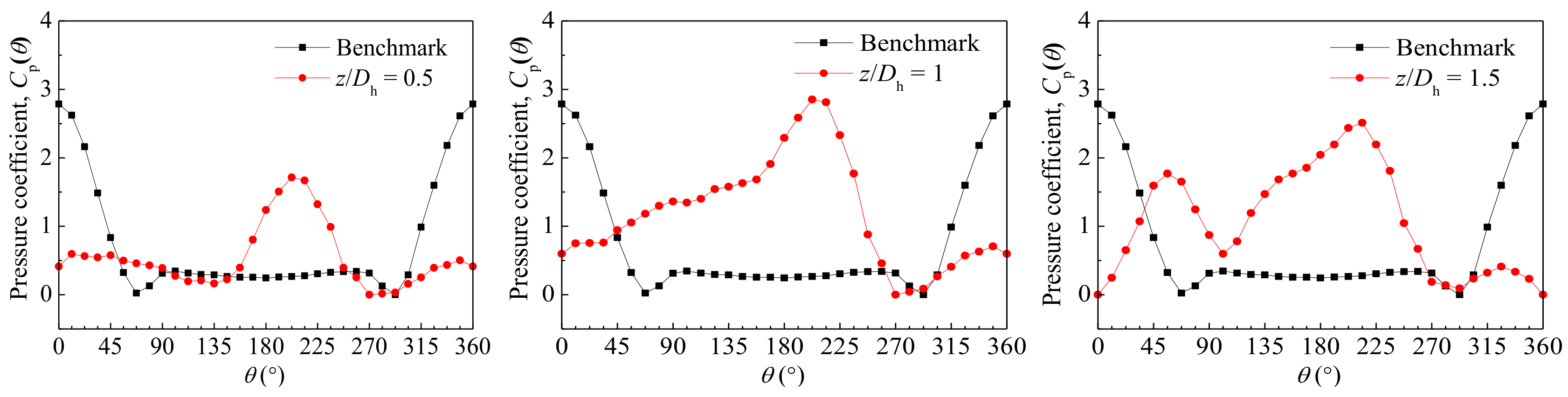
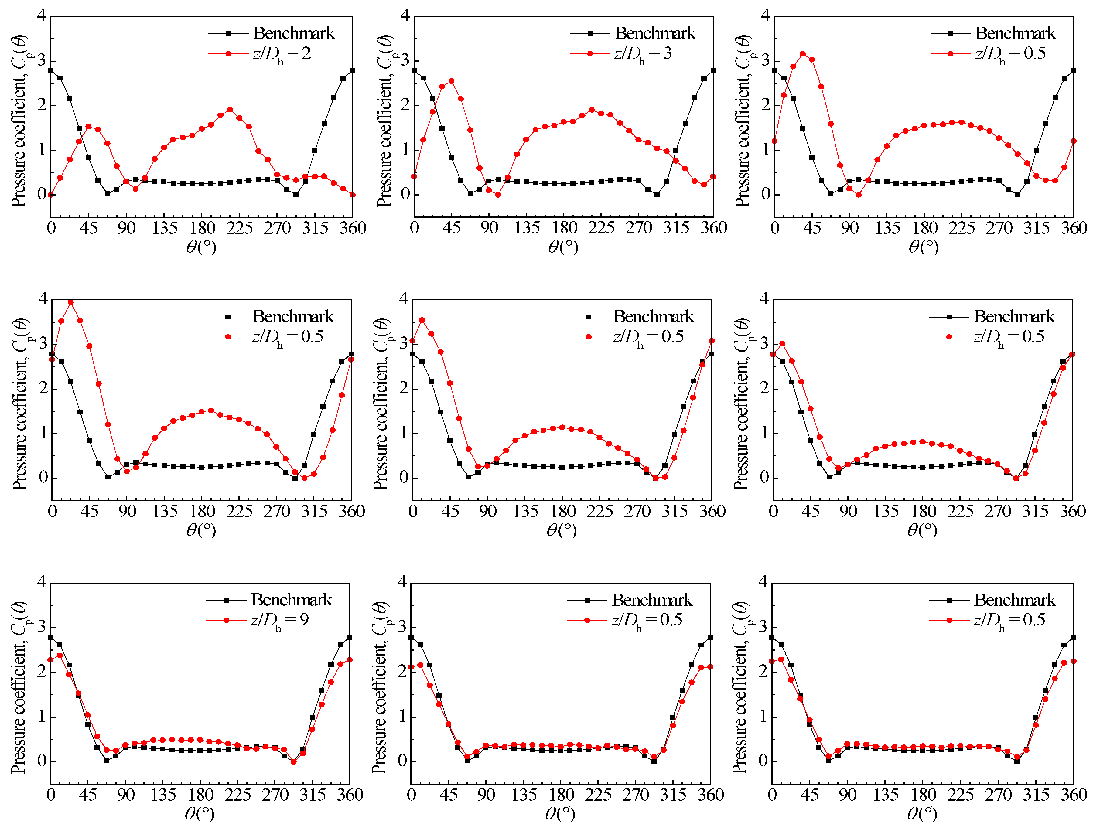
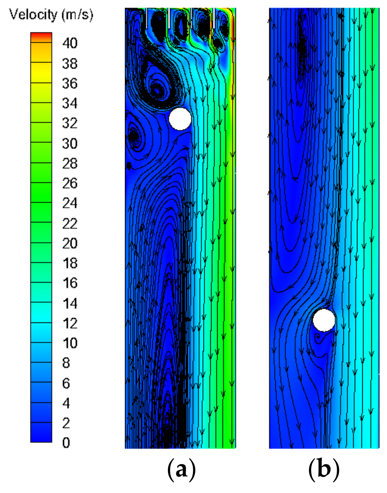
Figure 8 shows the typical test case of the pressure distributions at different positions under R = 0.117 without vanes and Figure 9 and Figure 10 are the corresponding numerical results, including the local and global flow structure. For the benchmark in Figure 8, the surface pressure distribution around the circular cylinder shows symmetry about the front stagnation point (θ = 0°) and rear stagnation point (θ = 180°) due to the uniformity of the oncoming flow in the straight duct. The peak value is about 2.8. From 0° to 180°, it monotonically declines until down to 0.0238 at the separation point at 67.5° where the flow boundary layer separation occurs and the adverse pressure gradient appears followed on. Finally it gradually decreases to a minimum value of 0.246 at 180°. However, in the T pipe junction, pressure distributions must be evidently asymmetric because of the intense non-uniformity of oncoming flow near the suction slot in T pipe junction and it would recover to the benchmark at the sufficient farther position as predicted. The changing process is shown as follows.
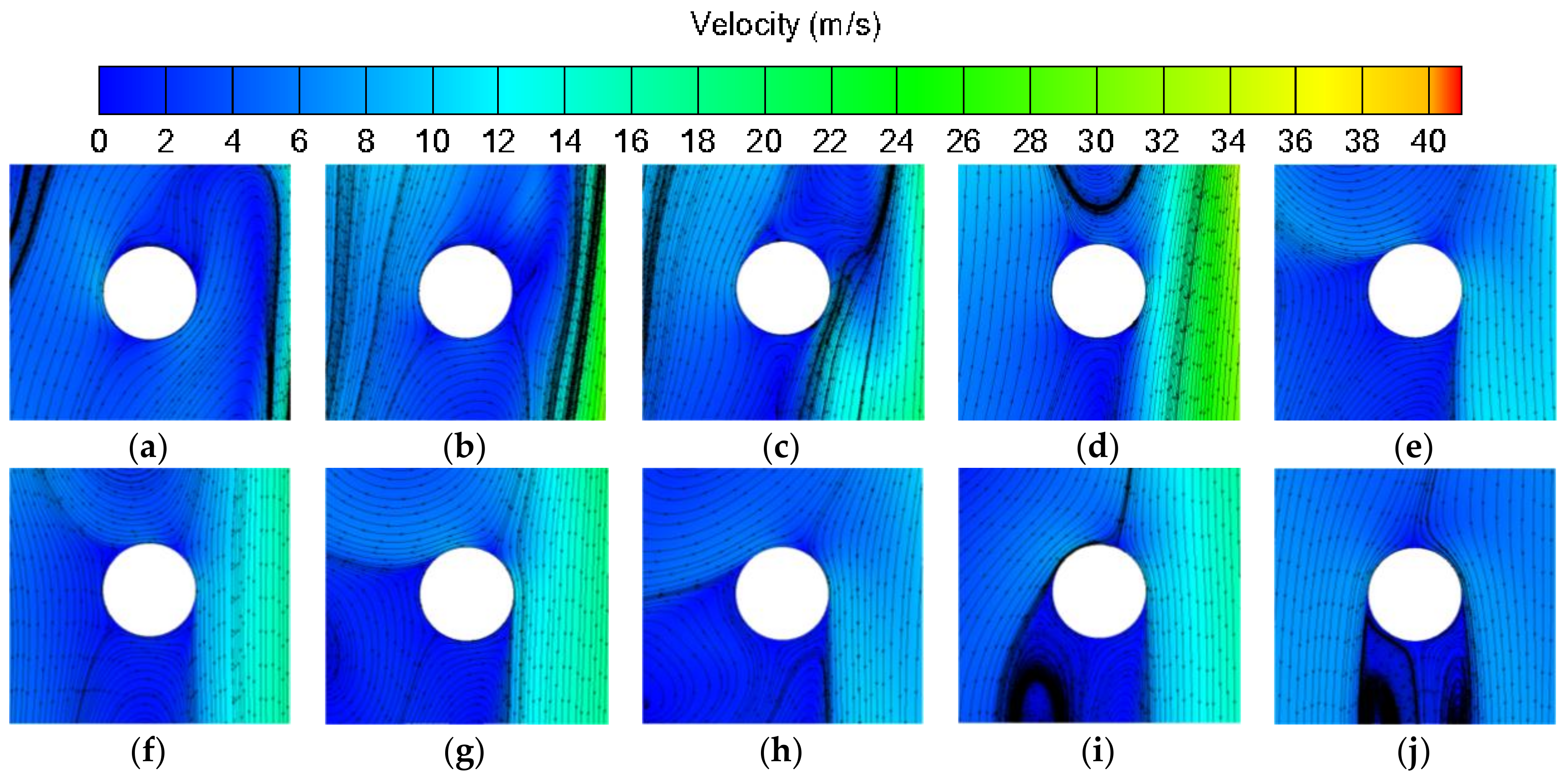
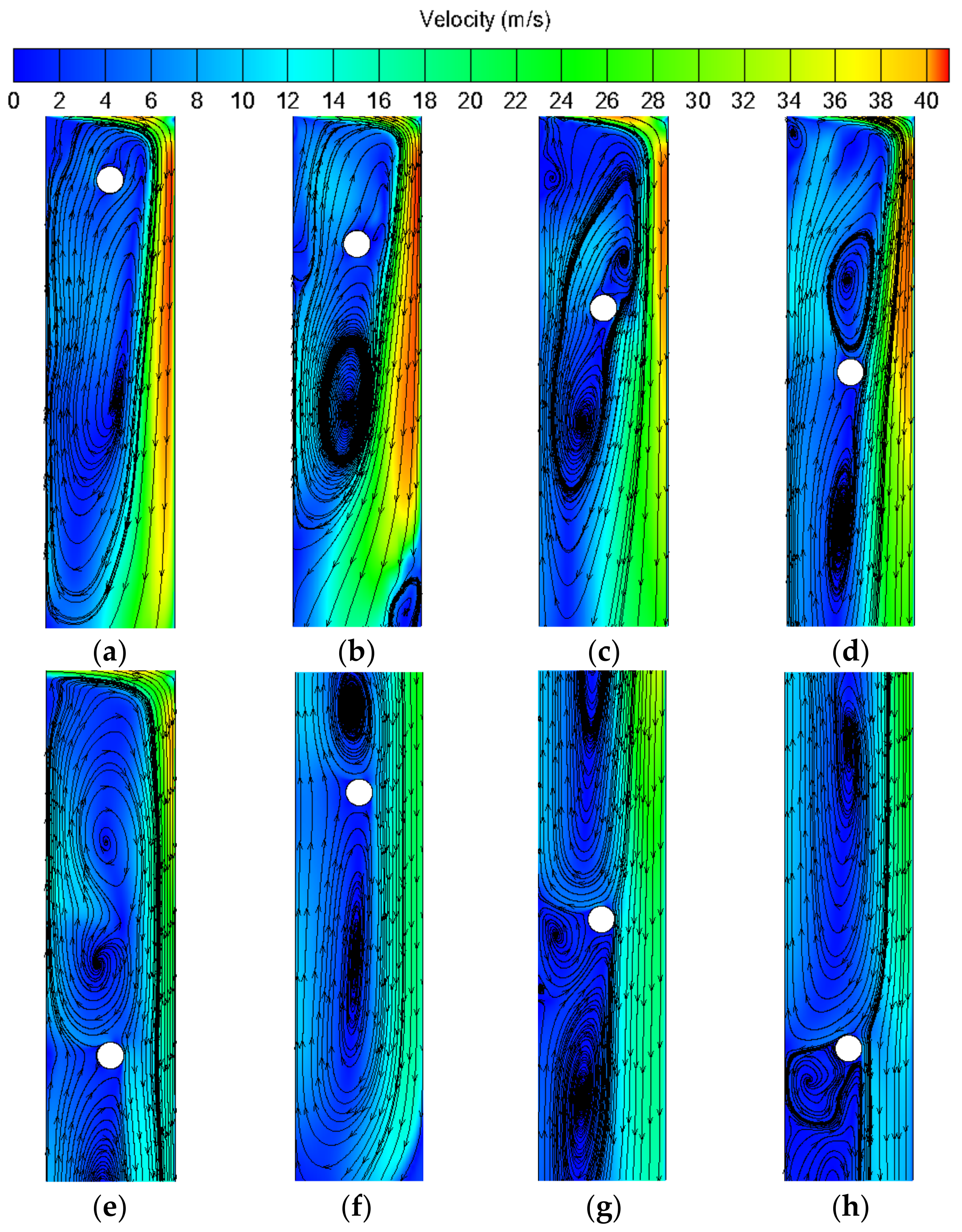
At z/Dh = 0.5, an obvious maximum point locates at about 203° with a value of about 1.71 and two minimum points at about 135° and 270° with values of about 0.28 and 0.32, respectively. This is because most part of the fluid flow through the right side of the suction and a “reverse oblique flow” past a cylinder forms which turns the front stagnation point from 0° to about 203° and the separation points from 67.5° and 292.5° to 135° and 270°, respectively, which can be seen in Figure 9a. Only a bit of change is exhibited in the range from 0° to 120° and 315° to 360°. It is expected that the reverse oblique reattachment flow of the free shear layer may be laminar and the vortices near this region may not become turbulent due to the relatively less and low speed fluid around the cylinder which locates at the upper side of the large vortex in the suction duct as can be seen in Figure 10a. Meanwhile, most part of the surface pressure coefficients are less than the benchmark except in the region near the front stagnation. At z/Dh = 1, the holistic pressure coefficients are greater than that at z/Dh = 0.5 especially the peak value at about 203°. A monotonous rise can be observed from 0° to 203°. Only one distinct separation point remains at 270°. Figure 9b and Figure 10b depict that the rear part of the reverse oblique flow past a cylinder becomes more complicated, and instead of the regular vortex street, and the upside cylinder has the tendency to form another vortex as can be seen in the farther positions. Here from z/Dh = 0.5 to z/Dh = 1, we define the single peak region, where the reverse oblique flow forms around and only one pressure peak value exists.
From z/Dh = 1.5 to z/Dh = 4, two peak values and separation points can be gradually observed. Their positions present a right offset relative to the benchmark as depicted in the curves. It can be seen from Figure 9c–f and Figure 10c–f that there are two obvious vortices above and below the circular cylinder in the suction duct. They are both encompassed in a large vortex. Each vortex carries the flow dynamic pressure on the cylinder so that two peak values generate at the stagnation points. The front stagnation value (near 0°) is smaller than the rear stagnation value (near 180°) at z/Dh = 1.5 and z/Dh = 2 while greater in the distance which change indicates the relative intensity of the two vortices.
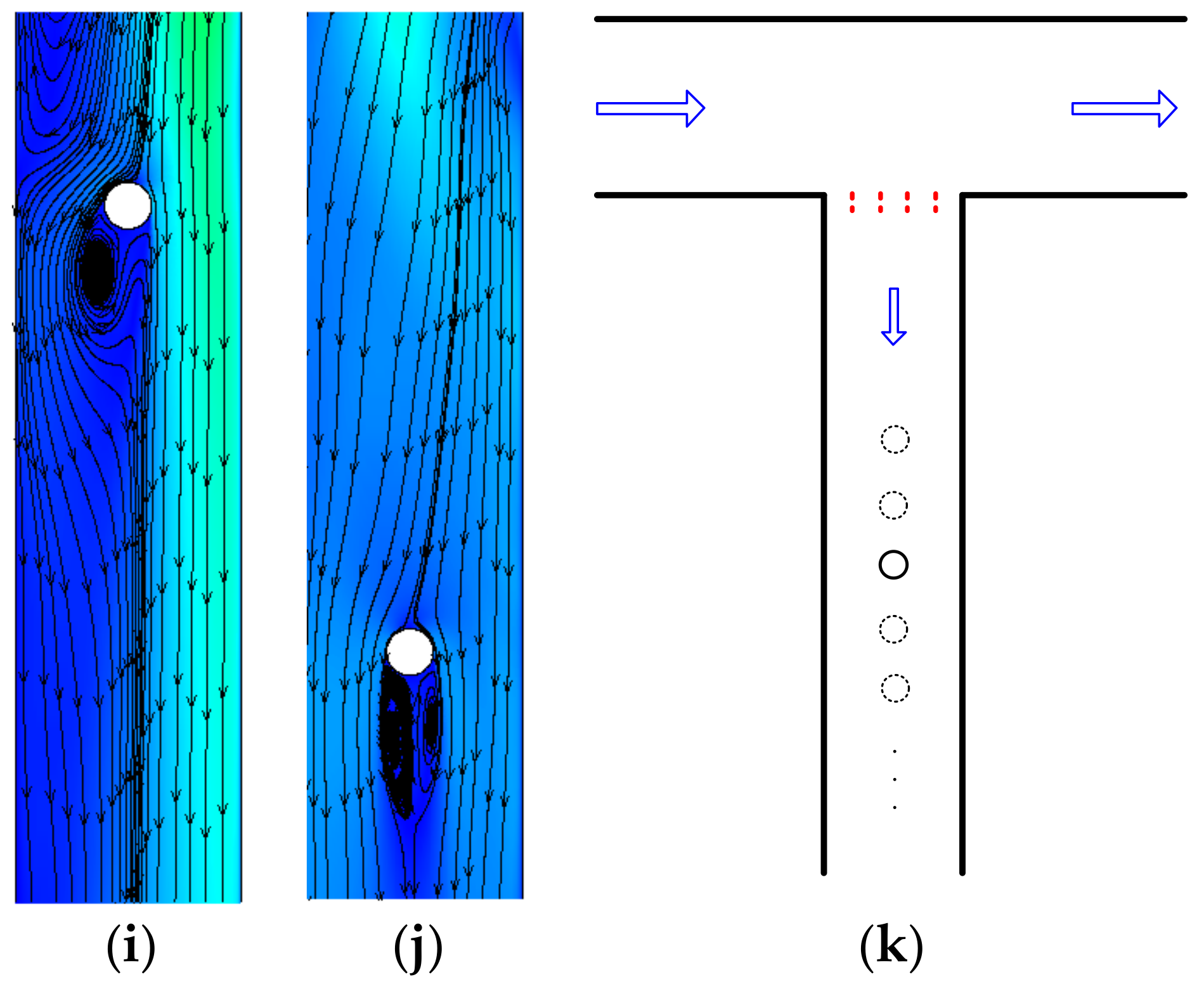
Here from z/Dh = 1.5 to z/Dh = 4, we define the double peaks region where double vortices form above and below the cylinder. From z/Dh = 5 we define the recovery region in which the pressure distribution starts to regain the benchmark gradually. This can be seen in Figure 9g–i and Figure 10g–i, where the immature vortex channel takes shape from z/Dh = 5 and finally forms at z/Dh = 9. At z/Dh = 9, the pressure coefficient curve becomes nearly symmetrical and it is very close to the benchmark curve at father distance though there are a bit of smaller points near 0°.
As analyzed before, three flow regions divided by the number of peak value are described and the front stagnation point, the rear stagnation point and the separation points are shown again from the double peaks region. Their changing law is as follows.
It can be seen from Figure 8 that the front stagnation point appears at about 203° at the single region due to “reverse oblique flow”. From the double peaks region, a right offset about 56° appears at z/Dh =1.5 and it shows gradual move back to 0° as the increase of z/Dh. The pressure coefficient value firstly increases and then decreases, finally maintaining around the benchmark. The largest value is even up to 3.96 at z/Dh = 5. The rear stagnation point firstly appears at about 214° at z/Dh = 1.5 with a value of 2.51. The peak value firstly decreases slowly and then turns into a more and more smooth region between the two separation points. It is almost the same from z/Dh = 11 with the benchmark. This is because both the intensity and the location of the above and below vortices around the cylinder keep constantly changing as the variation of z/Dh as depicted in Figure 10. It is expected that the vortices near the cylinder surface become intense first and then turn out to be weakened gradually with the increase of z/Dh, leading to the corresponding dynamic pressures exerted on the circular cylinder. The separation points show the relative opposite position at z/Dh = 0.5, with one point disappearing at z/Dh = 1 and recovering to two points from z/Dh = 1.5 as the flow direction around the circular cylinder transforms from reverse to obverse. They are between the two stagnation points and show a similar variation. From z/Dh = 1.5, the angle positions are moved back gradually from about 101° to 67.5° and about 349° to 292.5°, respectively.
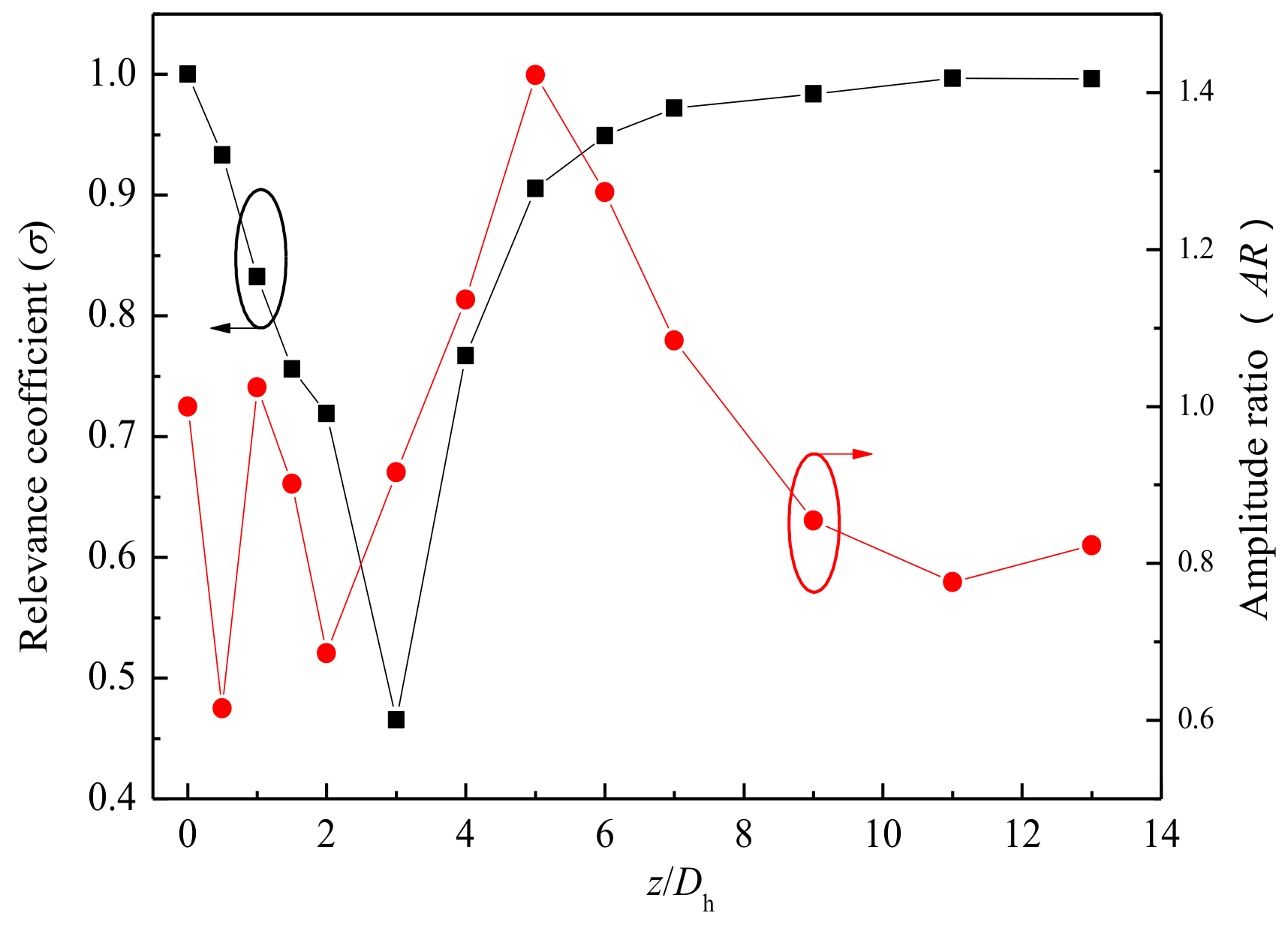
The above analyses are mainly around the local featured points. A general description of the pressure coefficient curve based on the relevance coefficient (σ) and amplitude ratio (AR), which are defined in Section 3.3, follows. The pressure coefficient curve is more similar to the benchmark when the relevance coefficient is approaching 1. The amplitude ratio can reflect the limit value of the pressure coefficient at one position.
Figure 11 shows the relevance coefficients and amplitude ratios at R = 0.117 without vanes. It is noted that z/Dh = 0 in x-coordinate denotes the benchmark with the values of 1 for both the relevance coefficient and amplitude ratio. The relevance coefficient firstly monotonically declines up to z/Dh = 3 with a minimum value of 0.47, and then increases gradually until close to the benchmark with the value of 1. It means that the effect of secondary flow for the suction duct gets more and more weakened. Some higher values exist at lower z/Dh. This is because the relevance coefficient is chosen from the maximum value of the 32 alternate calculations as defined in Equations (8) and (9) and the “reverse oblique flow” near the suction slot would more resemble with the benchmark at one certain alternate angle. Generally the amplitude ratio increase first and then decrease until to relative steady at last. Some irregular points appear from z/Dh = 0.5 to z/Dh = 2 mainly because the maximum value of pressure coefficients is in the range of θ > 180° from z/Dh = 0.5 to z/Dh = 2, while at the front stagnation point (θ < 90°) when z/Dh > 2 as can be seen in Figure 8. The largest value is up to 1.42 at z/Dh = 5.
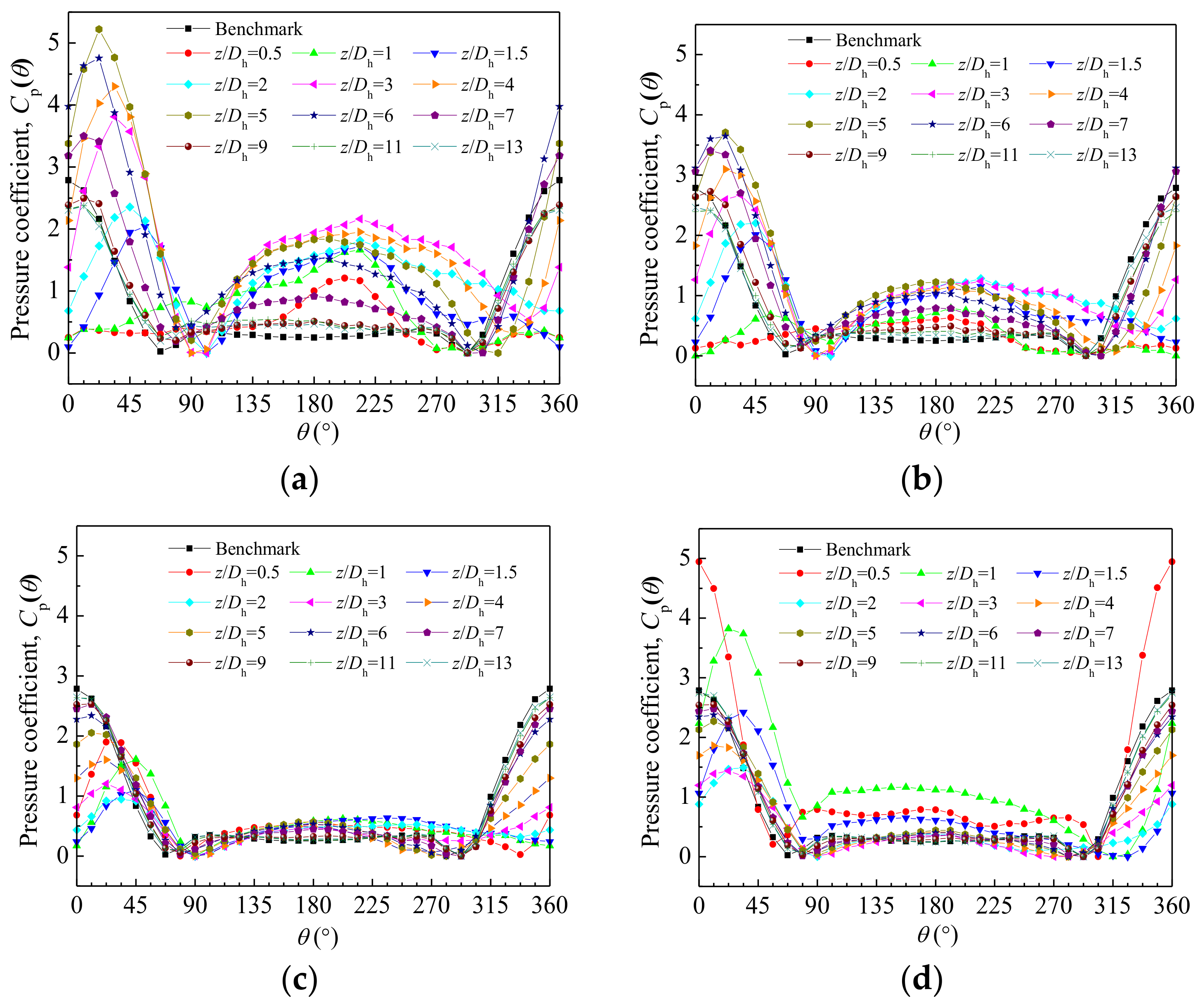
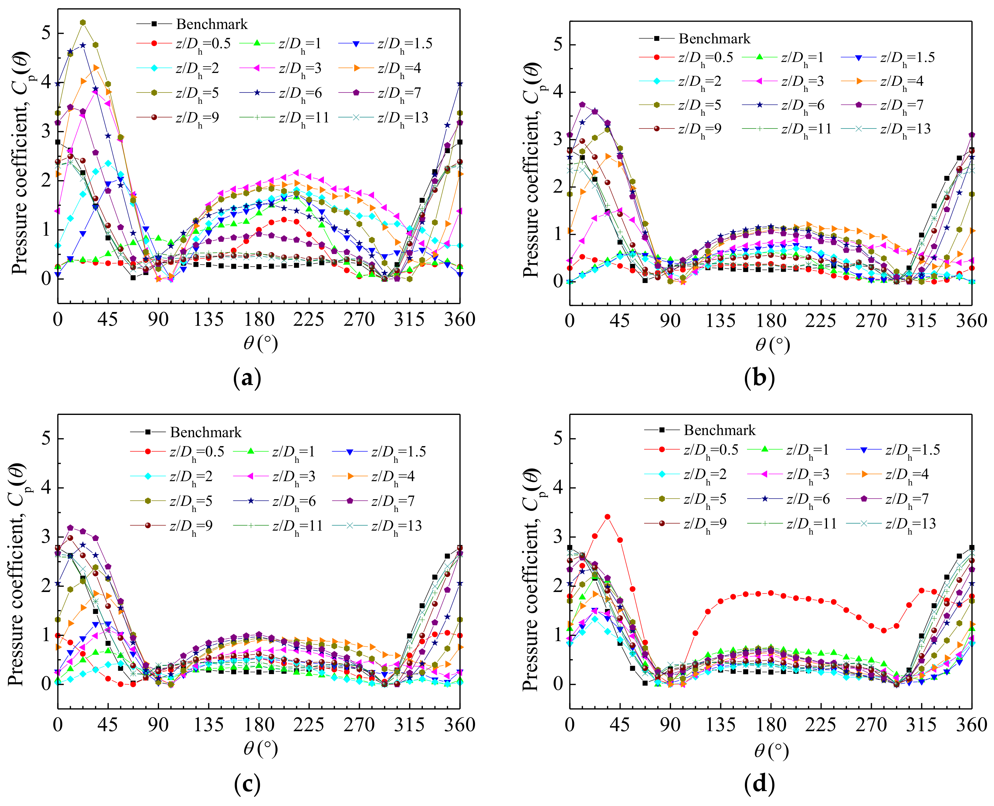
Figure 12 show the pressure distributions at other velocity ratios without vanes. Their relevance coefficients and amplitude ratios are depicted in Figure 13. Totally, as the velocity ratio increases, all the pressure coefficients show smaller values, especially the values in the front stagnation and rear stagnation regions as can be seen in Figure 12. Meanwhile, the single peak region appears more and more weakened. It can be seen obviously at R = 0.150, but not clearly at R = 0.263, and it disappears at R = 0.439 which presents the double peaks region directly. Left of Figure 13 shows that the recovery process to the benchmark gets more and more rapid. The locations of the minimum relevance coefficient approach to the suction entrance and the values become greater as the velocity ratio increases. All the relevance coefficients are larger than 0.97, very close to the benchmark, when z/Dh 7. For R = 0.614, the minimum value is already 0.9 and the pressure distribution curve is almost symmetrical at z/Dh = 0.5. That means the changes remain similar but the influence of the secondary flow on the suction duct gets more and more weakened at the larger velocity ratio. The amplitude ratios increase first and then decrease for R ≤ 0.263 while they decrease first and then increase for larger velocity ratios, as presented on the right of Figure 13.
5.2. Mean Pressure Distribution with Vanes
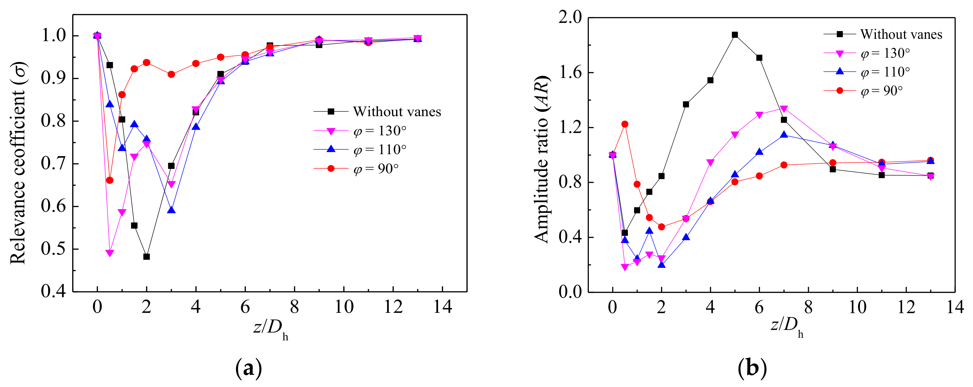
This section presents the experimental tests with vanes. Figure 14 shows the pressure distributions at R = 0.150 with the vanes angle in the range of 90° ≤ φ ≤ 130° and Figure 15 is the corresponding typical numerical results. Generally, it can be seen that the curves exhibit lower amplitude values around the circular cylinder, especially at the two stagnation points (regions) as the decrease of vanes angle compared to the case without vanes. That means the vanes help the branch recover to the benchmark and the smaller vanes angle, the faster recovery in the range of 90° ≤ φ ≤ 130°. When φ = 90°, all pressure distribution curves are much closer to the benchmark except at z/Dh = 0.5 with some higher values which maybe result from the strong flushing by the flow though the vanes, leading to the intense dynamic pressure exerted on the cylinder surface. It can be explained that the 90° mounted vanes parallel the streamline to the wall, prevent the upstream flow forming large vortices thus to weaken the strength of secondary flow as much as possible, as described in Figure 15. Figure 15a,c show that the cylinder is already located in the recovery region at z/Dh = 1 with 90° mounted vanes but still in the single peak region without vanes in Figure 14. It can be observed from Figure 16 that with the decrease of vane angle, the variation trend in relevance coefficients and amplitude ratios remains very familiar compared with that in Figure 13. It is expected that both the decrease of vanes angle and the increase of velocity ratio have a similar effect to weaken the suction influence and recover to the benchmark as soon as possible. The amplitude ratios from z/Dh = 0.5 to z/Dh = 2 with φ = 90° show higher values than other cases with vanes perhaps because some small vortices formed by the vanes still act on the circular cylinder strongly near the bifurcation.
5.3. Drag Coefficient (CD) and Lift Coefficient (CL)
The force conditions on the circular cylinder are analyzed in this part included the drag and lift coefficients which are defined before. Figure 17 shows the cases without vanes. Here z/Dh = 0 at x-coordinate denotes the drag and lift coefficients of the benchmark. From Figure 17a we can see that for a single velocity ratio, the drag coefficients decrease first and then increase as the far distance of z/Dh until gradually close to the benchmark and a minimum exists at about 1 < z/Dh < 1.5 and also the drag coefficients increase as the velocity ratio increases. It is noticed that the drag coefficients are less than zero at some positions when R ≤ 0.263. That means the resultant force on the circular cylinder in z-direction is upwards. It can be explained that the pressure coefficients around the down semi-cylinder (90°–180°–270°), especially at the rear stagnation region, are generally greater than that around the up semi-cylinder (270°–0°–90°) at these positions as shown in Figure 8 and Figure 12. It is expected that the strength of vortices behind the cylinder is stronger than that in front of the cylinder leading to the backflow. The smaller the velocity ratio, the intenser the backflow which results in the wider range of CD < 0. For R = 0.117, the minimum value at z/Dh = 1 is −1.33 which almost equals the benchmark for the absolute value. For R ≥ 0.439, all the drag coefficients are greater than zero, in the positive z-direction. The corresponding lift coefficients are depicted on Figure 17b. It can be observed that the lift coefficients curves are twist and turns. The peak values at about z/Dh = 2~3 are followed by the first minimums at about z/Dh = 1, and then the second minimums occur at z/Dh = 5 with the end of gradual recovery to the benchmark as the farther distance. It is pointed that the most of the lift coefficients are less than zero except some values at the peak regions. It indicates that the resultant force on the circular cylinder in x-direction is leftwards at most positions. Also it can be explained that the pressure coefficients around the right semi-cylinder (0°–180°), especially at the front stagnation region, are generally greater than that around the left semi-cylinder (180°–360°) as shown in Figure 8 and Figure 12. For R = 0.150, the maximum and minimum values are 0.21 at z/Dh = 2 and −0.74 at z/Dh = 5, respectively. For R = 0.614, all the lift coefficients are less than zero, in the negative x-direction.
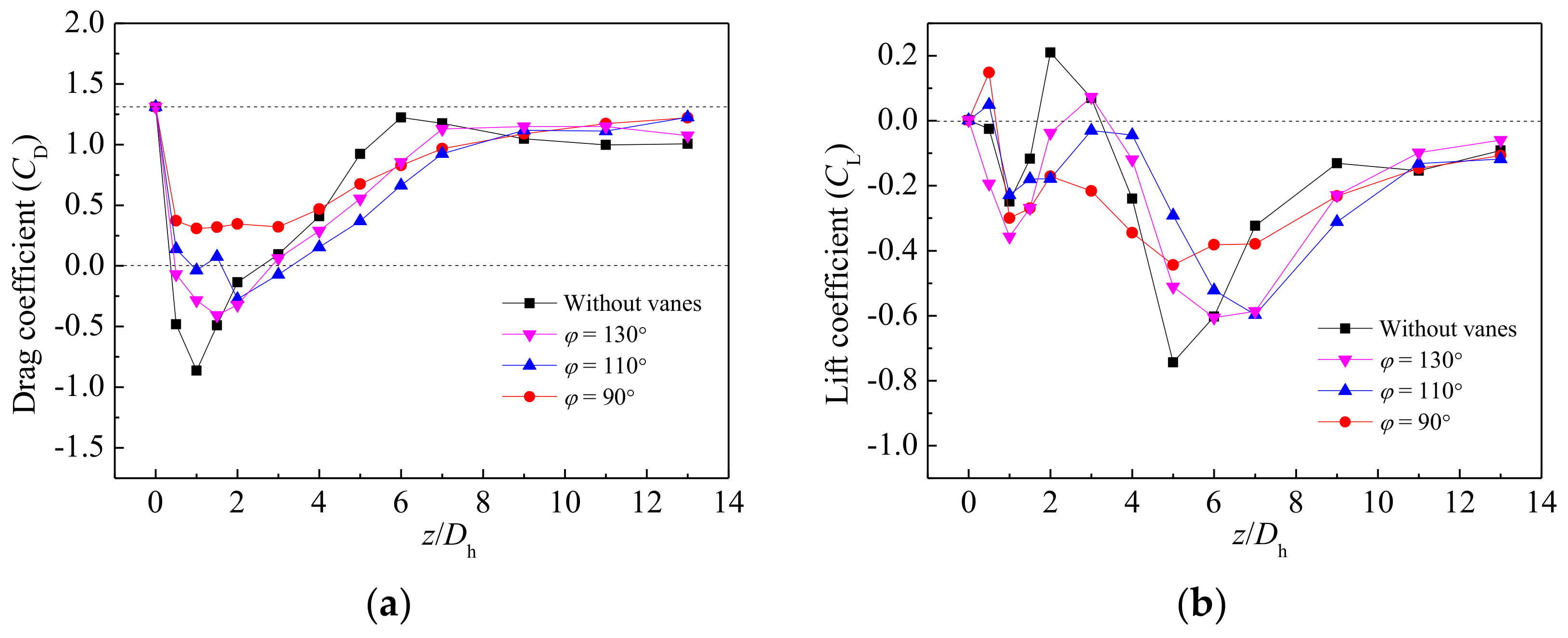
Figure 18 shows drag and lift coefficients at R = 0.150 with the vanes angle in the range of 90° ≤ φ ≤ 130°. It can be seen that as the decrease of vanes angle, the drag coefficients present higher values near the suction slot (z/Dh ≤ 4) and they are all greater than zero under φ = 90°. Meanwhile the lift coefficients present less fluctuation. This means that both the decrease of vanes angle and the increase of velocity ratio have the similar effect to make the circular cylinder with less force fluctuation.
6. Conclusions
Experimental and numerical investigations of force analysis acting on a single circular cylinder in the T pipe junction with the vanes effect are presented in this paper. The angle of the vanes is in the range of 90° ≤ φ ≤ 130°. One single benchmark experimental test in the extended suction duct (straight duct) is conducted beforehand to both verify the experimental method and compare the results with the data obtained in a T pipe junction. Numerical studies which are validated by the experimental data help understand the flow structure for the analysis. The main conclusions are as follows:
- (1)
- For a typical single velocity ratio R = 0.117 in the T pipe junction without vanes, influenced by the secondary flow in the suction duct, the cylinder presents different surface mean pressure distributions at the different positions including a single peak region, a double peaks region and a recovery region, which are analyzed in detail. As the distance from the junction to the cylinder center increases, the pressure distribution curves slowly recover to the benchmark value. Increasing the velocity ratio can make the single peak region and the double peaks region disappear gradually to speed up the recovery to the benchmark. The changing process of the main feature points including the front stagnation point, the rear stagnation point and the separation points are performed. Generally, increasing the velocity ratio can also increase the relevance coefficient. The amplitude ratios firstly increase and then decrease for R ≤ 0.263 while this is reversed for larger velocity ratios. For R = 0.614, the minimum relevance coefficient is already 0.9 and the pressure distribution curve is almost symmetrical at z/Dh = 0.5. That means the secondary flow effect on the suction duct is very small.
- (2)
- In the T pipe junction with vanes, all the pressure distribution curves exhibit lower amplitude values around the circular cylinder, especially at the two stagnation points (regions) as the decrease of vanes angle compared to the case without vanes. Both decreasing the vanes angle and increasing the velocity ratio have the same effect to weaken the suction flow and make the recovery to the benchmark faster.
- (3)
- For the test cases without vanes, the drag coefficients decrease first and then increase as the far distance of z/Dh until gradually close to the benchmark and they increase as the velocity ratio increases. The drag coefficients are less than zero at some positions when R ≤ 0.263 and the corresponding detailed analysis are presented. The lift coefficients curves are twists and turns and they are less than zero except some values at the peak regions which are also analyzed in detail. For the test cases with vanes, both the decrease of vanes angle and the increase of velocity ratio have a similar effect to make the circular cylinder display less force fluctuation.
Acknowledgements
We would like to acknowledge financial support for this work provided by the National Natural Science Foundation of China (Grant No. 51236003 and 51376145).
Author Contributions
Yantao Yin and Shicong Li conceived, designed and performed the experiments; Mei Lin contributed analysis tools; Liangbi Wang and Qiuwang Wang are the reviewers of this paper.
Conflicts of Interest
The authors declare no conflict of interest.
Nomenclature
| A | aspect ratio (l/d) |
| Am | main duct width (mm) |
| AR | amplitude ratio |
| B | block ratio (d/l) |
| CD | drag coefficient |
| CL | lift coefficient |
| Cp(θ) | pressure coefficient at θ degree |
| d | circular cylinder outer diameter (mm) |
| Dh | suction duct hydraulic diameter (mm) |
| fx | resultant force on unit length of circular cylinder in x-direction |
| fz | resultant force on unit length of circular cylinder in z-direction |
| F(δ) | correlation function |
| Hm | main duct height (mm) |
| Hv | vanes height (mm) |
| l | circular cylinder length (mm) |
| P(θ) | pressure value at θ degree (Pa) |
| Pmin | minimum pressure value (Pa) |
| P∞ | freestream static pressure (Pa) |
| Pr | Prandtl number |
| Q | volume flow rate (m3/s) |
| R | velocity ratio |
| r | circular cylinder radius (mm) |
| Re | Reynolds number |
| Res | Reynolds number for flow in suction duct |
| Rec | Reynolds number for flow past circular cylinder |
| S | cross-section area (m2) |
| V | bulk velocity (m/s) |
| Vsc | centerline velocity of suction duct (m/s) |
| x, y, z | Cartesian coordinate system (mm) |
| Greek symbols | |
| ∆ | thickness of vanes (mm) |
| δ | angle variation (°) |
| θ | circumferential angle around circular cylinder (°) |
| ρ | density (kg/m3) |
| σ | relevance coefficient |
| φ | angle of the vanes (°) |
| Subscripts | |
| i | side duct |
| m | main duct |
| s | suction duct |
| Superscripts | |
| B | benchmark |
| T | T pipe junction |
References
- Raghunathan, R.S.; Kim, H.D.; Setoguchi, T. Aerodynamics of high-speed railway train. Prog. Aeosp. Sci. 2002, 38, 469–514. [Google Scholar] [CrossRef]
- Williamson, C. Vortex dynamics in the cylinder wake. Annu. Rev. Fluid Mech. 1996, 28, 477–539. [Google Scholar] [CrossRef]
- Norberg, C. Fluctuating lift on a circular cylinder: Review and new measurements. J. Fluids Struct. 2003, 17, 57–96. [Google Scholar] [CrossRef]
- Shao, J.; Zhang, C. Numerical analysis of the flow around a circular cylinder using RANS and LES. Int. J. Comput. Fluid D 2006, 20, 301–307. [Google Scholar] [CrossRef]
- Sayeed-Bin-Asad, S.M.; Lundström, T.S.; Andersson, A.G. Study the flow behind a semi-circular step cylinder (laser doppler velocimetry (LDV) and computational fluid dynamics (CFD)). Energy 2017, 10, 332–344. [Google Scholar] [CrossRef]
- Anagnostopoulos, P.; Iliadis, G.; Richardson, S. Numerical study of the blockage effects on viscous flow past a circular cylinder. Int. J. Numer. Meth. Fluids 1996, 22, 1061–1074. [Google Scholar] [CrossRef]
- Szepessy, S.; Bearman, P.W. Aspect ratio and end plate effects on vortex shedding from a circular cylinder. J. Fluid Mech. 1992, 234, 191–217. [Google Scholar] [CrossRef]
- Schewe, G. On the force fluctuations acting on a circular cylinder in cross-flow from subcritical up to transcritical Reynolds numbers. J. Fluid Mech. 1983, 133, 265–285. [Google Scholar] [CrossRef]
- Sumer, B.M.; Fredsøe, J. Hydrodynamics around Cylindrical Structures; World Sci.: Singapore, 1997. [Google Scholar]
- West, G.S.; Apelt, C.J. The effects of tunnel blockage and aspect ratio on the mean flow past a circular cylinder with Reynolds numbers between 104 and 105. J. Fluid Mech. 1982, 114, 361–377. [Google Scholar] [CrossRef]
- Allen, H.J.; Vincenti, W.G. Wall Interference in a Two-Dimensional-Flow Wind Tunnel, with Consideration of the Effect of Compressibility; NACA report 782; National Aeronautics and Space Administration Moffett Field Ca Ames Research Center: Mountain View, CA, USA, 1944. [Google Scholar]
- Maskell, E.C. A Theory of the Blockage Effect on Bluff Bodies and Stalled Wings in Closed Tunnel; ARC R&M 3400; Aeronautical Research Council: London, UK, 1963. [Google Scholar]
- Cantwell, B.; Coles, D. An experimental study of entrainment and transport in the turbulent near wake of a circular cylinder. J. Fluid Mech. 1983, 136, 321–374. [Google Scholar] [CrossRef]
- Norberg, C. An experimental investigation of the flow around a cirucular cylinder: Influence of aspect ratio. J. Fluid Mech. 1994, 258, 287–316. [Google Scholar] [CrossRef]
- Tsutsui, T.; Igarashi, T. Drag reduction of a circular cylinder in an air-stream. J. Wind Eng. Ind. Aerodyn. 2002, 90, 527–541. [Google Scholar] [CrossRef]
- Bearman, P.W. On vortex shedding from a circular cylinder in the critical Reynolds number regime. J. Fluid Mech. 1969, 37, 577–585. [Google Scholar] [CrossRef]
- Achenbach, E. Distribution of local pressure and skin friction around a circular cylinder in cross-flow up to Re=5×10⁶. J. Fluid Mech. 1968, 34, 625–639. [Google Scholar] [CrossRef]
- Shih, W.C.; Wang, C.; Coles, D.; Roshko, A. Experiments on flow past rough circular cylinders at large Reynolds numbers. J. Wind Eng. Ind. Aerodyn. 1993, 49, 351–368. [Google Scholar] [CrossRef]
- Breuer, M. Large eddy simulation of the sub-critical flow past a circular cylinder. Int. J. Heat Fluid Flow 1998, 28, 1281–1302. [Google Scholar]
- Kravchenko, A.G.; Moin, P. Numerical studies of flow over a circular cylinder at ReD=3900. Phys. Fluids 2000, 12, 403–417. [Google Scholar] [CrossRef]
- Ünal, U.O.; Atlar, M.; Gören, O. Effect of turbulence modelling on the computation of the near-wake flow of a circular cylinder. Ocean Eng. 2010, 37, 387–399. [Google Scholar] [CrossRef]
- Yeon, S.M.; Yang, J.M.; Stern, F. Large-eddy simulation of the flow past a circular cylinder at sub- to super-critical Reynolds numbers. Appl. Ocean Res. 2016, 59, 663–675. [Google Scholar] [CrossRef]
- Lloyd, T.P.; James, M. Large eddy simulations of a circular cylinder at Reynolds numbers surrounding the drag crisis. Appl. Ocean Res. 2016, 59, 676–686. [Google Scholar] [CrossRef]
- Catalano, P.; Wang, M.; Iaccarino, G.; Moin, P. Numerical simulation of the flow around a circular cylinder at high Reynolds numbers. Int. J. Heat Fluid Flow 2003, 24, 463–469. [Google Scholar] [CrossRef]
- Ong, M.C.; Utnes, T.; Holmedal, L.E.; Myrhaug, D.; Pettersen, B. Numerical simulation of flow around a smooth circular cylinder at very high Reynolds numbers. Mar. Struct. 2009, 22, 142–153. [Google Scholar] [CrossRef]
- Melling, A.; Whitelaw, J.H. Turbulent flow in a rectangular duct. J. Fluid Mech. 1976, 78, 289–315. [Google Scholar] [CrossRef]
- Kline, S.J.; Mcclintock, F.A. Describing uncertainties in single-sample experiments. >Mech. Eng. 1953, 75, 3–8. [Google Scholar]
- Norberg, C.; Sunden, B. Turbulence and Reynolds number effects on the flow and fluid forces on a single cylinder in cross flow. J. Fluids Struct. 1987, 1, 337–357. [Google Scholar] [CrossRef]
- Ahmed, M.R.; Talama, F. Flow characteristics and local heat transfer rates for a heated circular cylinder in a cross flow of air. Int. J. Fluid Mech. Res. 2008, 35, 76–93. [Google Scholar] [CrossRef]
- Franke, J.; Hirsch, C.; Jensen, A.G.; Krüs, H.W.; Schatzmann, M.; Westbury, P.S.; Miles, S.D.; Wisse, J.A.; Wright, N.G. Recommendations on the use of CFD in wind engineering. In Proceedings of the International Conference on Urban Wind Engineering and Building Aerodynamics, Sint-Genesius-Rode Belgium, 5–7 May 2004. [Google Scholar]
- Menter, F.R. Two-equation eddy-viscosity turbulence models for engineering applications. AIAA J. 1994, 32, 1598–1605. [Google Scholar] [CrossRef]
Figure 1.
Abstract models of the ventilation and heat transfer units in the high speed train: (a) practical physical model; (b) simplified experimental model.
Figure 1.
Abstract models of the ventilation and heat transfer units in the high speed train: (a) practical physical model; (b) simplified experimental model.

Figure 2.
Schematic diagram of experimental test: (1) Entrance; (2) Transition section; (3) Contraction section; (4) Main duct; (5) Side duct; (6) Flow metering duct; (7) Expansion section; (8) Blower; (9) Test section; (10) Valve; (11) Rotor flowmeter; (12) Pitot tube; (13) Data acquisition system.

Figure 3.
2D illustration of the T pipe junction: (a) planar graph; (b) vanes structure.

Figure 4.
Details of the test cylinder and the angle around the cylinder surface: (a) the circular cylinder; (b) pressure taps; (c) angle around the circular cylinder surface.
Figure 4.
Details of the test cylinder and the angle around the cylinder surface: (a) the circular cylinder; (b) pressure taps; (c) angle around the circular cylinder surface.

Figure 5.
Validation of the experimental method.

Figure 6.
Computational domain in numerical investigation.

Figure 7.
Comparisons between CFD results with experimental measurements. (a) With vanes, R = 0.150, φ = 90°; (b) and (c) Without vanes, R = 0.117 and R = 0.150 and 0.263.
Figure 7.
Comparisons between CFD results with experimental measurements. (a) With vanes, R = 0.150, φ = 90°; (b) and (c) Without vanes, R = 0.117 and R = 0.150 and 0.263.
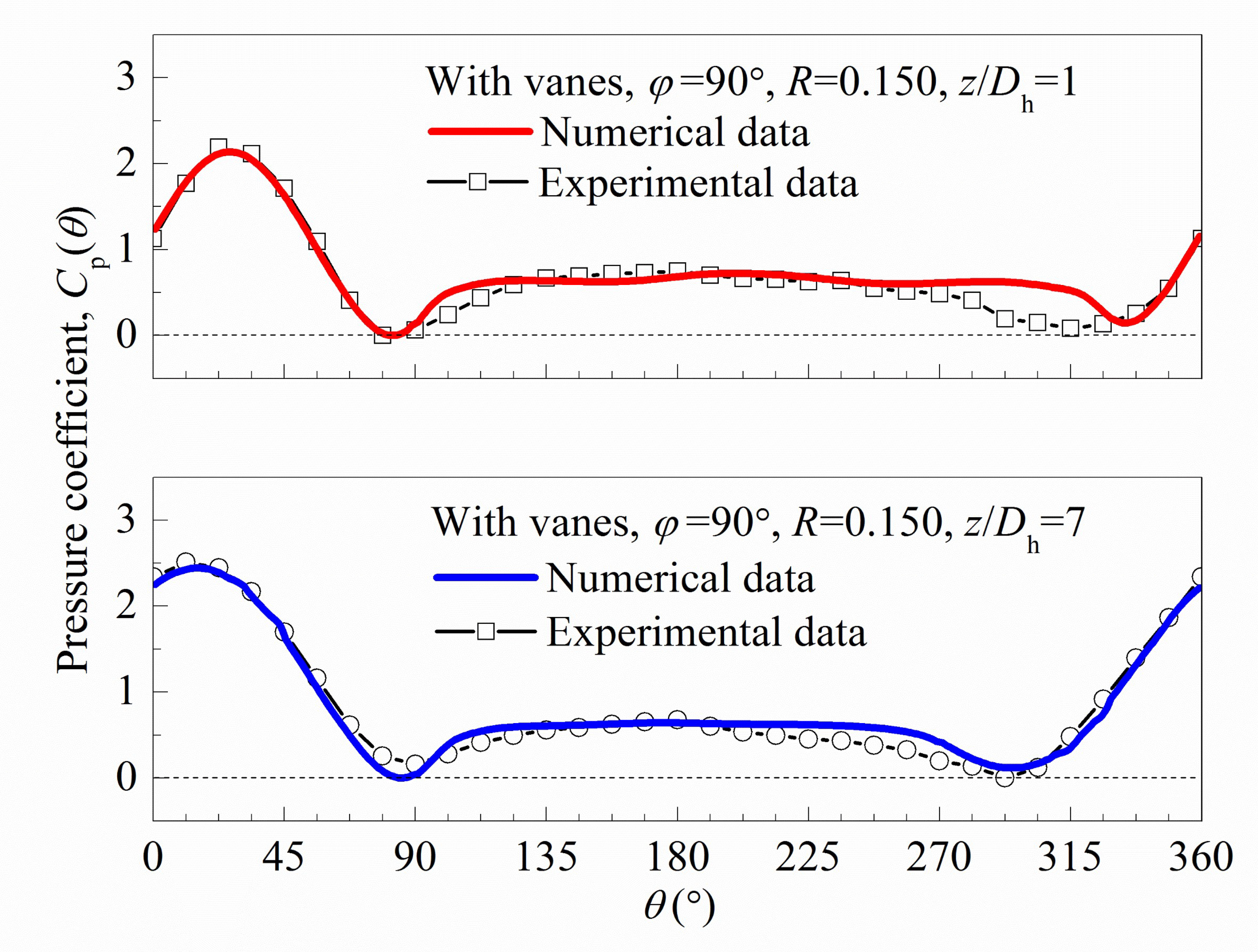

Figure 8.
Pressure distributions at different positions at R = 0.117 without vanes.


Figure 9.
Local flow structure around the circular cylinder at R = 0.117 without vanes: (a) z/Dh = 0.5; (b) z/Dh = 1; (c) z/Dh = 1.5; (d) z/Dh = 2; (e) z/Dh = 3; (f) z/Dh = 4; (g) z/Dh = 5; (h) z/Dh = 6; (i) z/Dh = 7; (j) z/Dh = 9.
Figure 9.
Local flow structure around the circular cylinder at R = 0.117 without vanes: (a) z/Dh = 0.5; (b) z/Dh = 1; (c) z/Dh = 1.5; (d) z/Dh = 2; (e) z/Dh = 3; (f) z/Dh = 4; (g) z/Dh = 5; (h) z/Dh = 6; (i) z/Dh = 7; (j) z/Dh = 9.

Figure 10.
Global flow structure around the circular cylinder at R = 0.117 without vanes: (a) z/Dh = 0.5; (b) z/Dh = 1; (c) z/Dh = 1.5; (d) z/Dh = 2; (e) z/Dh = 3; (f) z/Dh = 4; (g) z/Dh = 5; (h) z/Dh = 6; (i) z/Dh = 7; (j) z/Dh = 9 and (k) schematic figure of the T pipe junction.
Figure 10.
Global flow structure around the circular cylinder at R = 0.117 without vanes: (a) z/Dh = 0.5; (b) z/Dh = 1; (c) z/Dh = 1.5; (d) z/Dh = 2; (e) z/Dh = 3; (f) z/Dh = 4; (g) z/Dh = 5; (h) z/Dh = 6; (i) z/Dh = 7; (j) z/Dh = 9 and (k) schematic figure of the T pipe junction.


Figure 11.
Relevance coefficients and amplitude ratios at R = 0.117 without vanes.

Figure 12.
Pressure distributions at different positions at different R without vanes: (a) R = 0.150; (b) R = 0.263; (c) R = 0.439; (d) R = 0.614.
Figure 12.
Pressure distributions at different positions at different R without vanes: (a) R = 0.150; (b) R = 0.263; (c) R = 0.439; (d) R = 0.614.

Figure 13.
Relevance coefficients (left) and amplitude ratios (right) under different R without vanes.
Figure 13.
Relevance coefficients (left) and amplitude ratios (right) under different R without vanes.
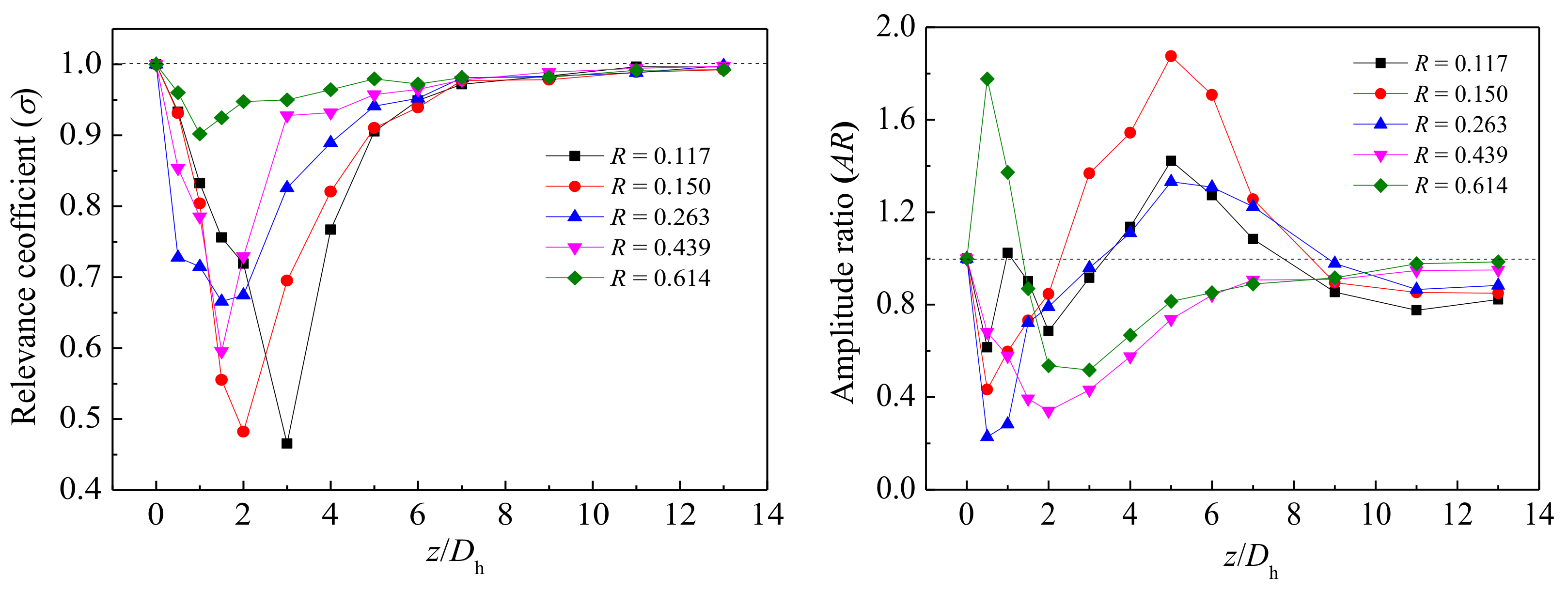
Figure 14.
Pressure distributions at different positions with different angle of the vanes at R = 0.150: (a) without vanes; (b) φ = 130°; (c) φ = 110°; (d) φ = 90°.
Figure 14.
Pressure distributions at different positions with different angle of the vanes at R = 0.150: (a) without vanes; (b) φ = 130°; (c) φ = 110°; (d) φ = 90°.

Figure 15.
Typical global and local flow structure around the circular cylinder at R = 0.150 with vanes: (a) global z/Dh = 1; (b) global z/Dh = 7; (c) local z/Dh = 1; (d) local z/Dh = 7.
Figure 15.
Typical global and local flow structure around the circular cylinder at R = 0.150 with vanes: (a) global z/Dh = 1; (b) global z/Dh = 7; (c) local z/Dh = 1; (d) local z/Dh = 7.

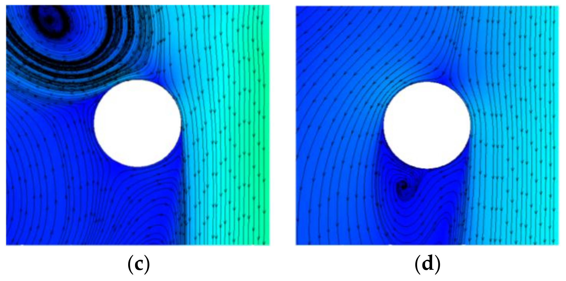
Figure 16.
Relevance coefficients (a) and amplitude ratios (b) with different angle of the vanes at R = 0.150.
Figure 16.
Relevance coefficients (a) and amplitude ratios (b) with different angle of the vanes at R = 0.150.

Figure 17.
Drag coefficients (a) and lift coefficients (b) at different R without vanes.
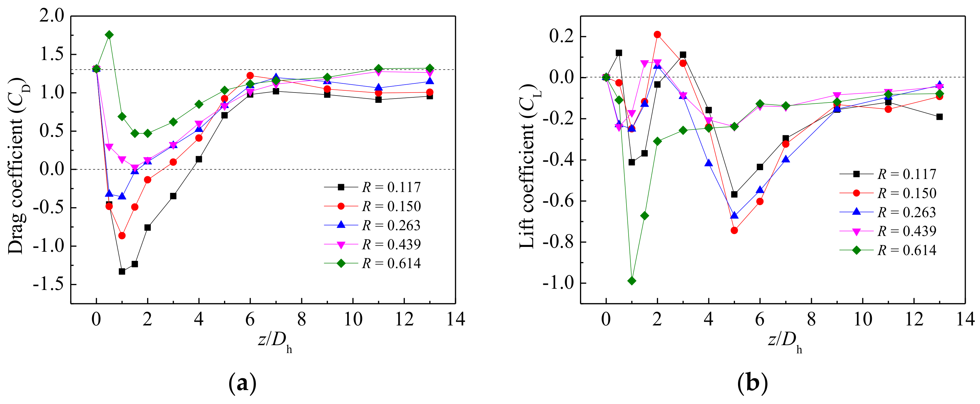
Figure 18.
Drag coefficients (a) and lift coefficients (b) with different angle of the vanes at R = 0.150.
Figure 18.
Drag coefficients (a) and lift coefficients (b) with different angle of the vanes at R = 0.150.

Table 1.
Comparisons of the drag coefficient between present result and West and Apelt [10].
Table 1.
Comparisons of the drag coefficient between present result and West and Apelt [10].
| CD | Reynolds Number | Blockage | Aspect Ratio |
|---|---|---|---|
| 1.352 (West and Apelt [10]) | 1.53 × 10⁴ | 16% | 4 |
| 1.381 (West and Apelt [10]) | 4.5 × 10⁴ | 15.8% | 6 |
| 1.310 (present) | 0.916 × 10⁴ | 20.1% | 4.78 |
Table 2.
Detail settings in three-dimensional CFD simulation.
| General Setting | Incompressible Fluid, Steady, Turbulent |
|---|---|
| Fluid material | Air with constant physical property |
| Turbulent model | SST k- [30,31] |
| Solution methods | Pressure-velocity coupling algorithm: SIMPLE |
| Gradient discretize: Least squares cell based | |
| Pressure discretize: Standard | |
| Other terms: Second order upwind | |
| Boundary conditions | Inlet of main duct: Constant velocity-inlet |
| Outs of suction and main ducts: Outflow | |
| Other surfaces: No slip wall |
© 2018 by the authors. Licensee MDPI, Basel, Switzerland. This article is an open access article distributed under the terms and conditions of the Creative Commons Attribution (CC BY) license (http://creativecommons.org/licenses/by/4.0/).
Share and Cite
MDPI and ACS Style
Yin, Y.; Li, S.; Wang, L.; Lin, M.; Wang, Q. Force Analysis of a Circular Cylinder at Ununiformed Flow in a T Pipe Junction. Energies 2018, 11, 864. https://doi.org/10.3390/en11040864
AMA Style
Yin Y, Li S, Wang L, Lin M, Wang Q. Force Analysis of a Circular Cylinder at Ununiformed Flow in a T Pipe Junction. Energies. 2018; 11(4):864. https://doi.org/10.3390/en11040864
Chicago/Turabian StyleYin, Yantao, Shicong Li, Liangbi Wang, Mei Lin, and Qiuwang Wang. 2018. "Force Analysis of a Circular Cylinder at Ununiformed Flow in a T Pipe Junction" Energies 11, no. 4: 864. https://doi.org/10.3390/en11040864
Note that from the first issue of 2016, this journal uses article numbers instead of page numbers. See further details here.