Short-Term Wind Power Forecasting Based on Clustering Pre-Calculated CFD Method

Abstract

To meet the increasing wind power forecasting (WPF) demands of newly built wind farms without historical data, physical WPF methods are widely used. The computational fluid dynamics (CFD) pre-calculated flow fields (CPFF)-based WPF is a promising physical approach, which can balance well the competing demands of computational efficiency and accuracy. To enhance its adaptability for wind farms in complex terrain, a WPF method combining wind turbine clustering with CPFF is first proposed where the wind turbines in the wind farm are clustered and a forecasting is undertaken for each cluster. K-means, hierarchical agglomerative and spectral analysis methods are used to establish the wind turbine clustering models. The Silhouette Coefficient, Calinski-Harabaz index and within-between index are proposed as criteria to evaluate the effectiveness of the established clustering models. Based on different clustering methods and schemes, various clustering databases are built for clustering pre-calculated CFD (CPCC)-based short-term WPF. For the wind farm case studied, clustering evaluation criteria show that hierarchical agglomerative clustering has reasonable results, spectral clustering is better and K-means gives the best performance. The WPF results produced by different clustering databases also prove the effectiveness of the three evaluation criteria in turn. The newly developed CPCC model has a much higher WPF accuracy than the CPFF model without using clustering techniques, both on temporal and spatial scales. The research provides supports for both the development and improvement of short-term physical WPF systems.

1. Introduction

In the context of the worldwide energy crisis and the urgent need to decarbonize electricity generation, the development of renewable energy has become central to energy policy [1]. Being one of the most mature clean energy technologies, wind energy is now widely used for power generation and is making a significant contribution to the electric power system [2,3]. However, due to the intermittent and time varying characteristics of wind energy, the integration of large-scale wind power into the electricity grid poses significant challenges to the safe and stable operation of power systems [4]. Accurate wind power forecasting (WPF) is an effective way to alleviate this problem since power system operators can then anticipate the wind power production in advance and plan accordingly. In addition, by reducing the uncertainty associated with wind power generation, forecasting can improve the market competitiveness of wind power [5,6].

WPF techniques are mature and widely used; they can be divided into statistical and physical methods [7]. The statistical WPF methods make use of a range of statistical prediction algorithms (neural networks, fuzzy logic, support vector machine and others) and are capable of predicting the wind power with high accuracy for limited look ahead periods [8,9]. However, a large amount of operational data is needed to establish such statistical WPF models, which precludes their application for newly constructed wind farms for which such data is lacking [10]. Physically-based WPF methods adopt the concepts of atmospheric dynamics and boundary-layer meteorology to carry out spatial refinement of coarse meso-scale numerical weather prediction (NWP) systems [11] to the specific site conditions as well as the transformation of the predicted wind speed to the hub height of wind turbines; they use only very limited historical data and can be applied to newly constructed wind farms [12]. Diagnostic and computational fluid dynamics (CFD) models are two basic classes of physical WPF systems. Diagnostic models [13] are based on the parameterizations of boundary layer without further dynamical information and are normally used for the modeling of flow over flat terrain. CFD models can dynamically simulate the relevant wind flow fields and deliver higher accuracy and are suitable for flow modeling in complex terrain [14]. Marjanovic et al. [15] have investigated the effects of model parameters on high-resolution WPF and the results imply that forecasting accuracy with complex terrain is more sensitive to the model’s spatial resolution than in the case of flat terrain. Murali et al. [16] use the Navier-Stokes equations with mixed basis formulations to simulate the interaction of multiple wind turbines located in complex terrain and demonstrate good agreement with the field measurements.

The CFD simulation of a wind farm flow fields includes both terrain modeling and wake modeling; the terrain and wake effects can be combined in two different ways [17]. One is the coupling of CFD simulation with full-scale or simplified wind turbine modeling [18,19], and the other is the superposition of CFD terrain simulation and semi-empirical engineering wake models [20]. According to different turbulence scales, terrain effects can be simulated by Reynold averaged Navier-Stokes (RANS), detached eddy simulation (DES) or large eddy simulation (LES) methods, among which the computation load varies considerably as the precision does [21]. According to Sanderse [22], for the applications like wind turbine layout optimization and wind power estimation, which focus on averaged wind velocities in wind turbine far wake area, the superposition of turbulent kinetic energies and velocity deficits is the most popular approach. Therefore, to speed up the modeling process, the fastest RANS model and the simplest engineering wake model should be adopted to calculate the terrain effects and wake effects, respectively.

However, even using the simplified superposition schemes of wind farm flow field simulation, the CFD modelling of the flow over complex terrain still has a heavy computational burden [21], which is unable to meet the timeliness requirements of short-term WPF [23]. In view of this, Li et al. [24,25] have devised a short-term WPF method based on CFD pre-calculated flow fields (CPFF), which allows the CFD calculations to be completed prior to the forecasting analysis, and saved in a flow characteristics database. Then meso-scale NWP data is used as input to the established database to predict the wind power for different future time periods. The CPFF-based WPF method dramatically reduces the time needed by the forecasting process and provides a good balance between computation time and forecasting accuracy.

Nevertheless, for wind farms located in complex terrain or covering large spatial extents, the elevations of different wind turbines can vary considerably. The CPFF method outlined above uses extrapolation from a single virtual mast to estimate the wind speeds at all wind turbine locations; it is unable to accurately represent the wind speeds across the entire wind farm, and this limits the power prediction accuracy [26]. Since it is also unrealistic to establish an individual forecasting model for each of the wind turbines in a wind farm, the compromise based on wind turbine clustering is seen as attractive [27]. In such an approach, as developed here for the first time, a clustering flow field database can be established, where wind turbines in the wind farm are classified into a few clusters and a forecasting model is made for each cluster.

Clustering methods have been widely used in many research areas, the commonly used clustering methods can be divided into partitioning-based, hierarchical-based, density-based, model-based and graph-based clustering [28]. Each category has its own clustering characteristics and application fields, and some clustering techniques have already been applied to wind power analysis and forecasting. Yan et al. [29] developed a clustering approach to WPF based on the combination of a model-based self-organizing feature mapping clustering approach and a statistical forecasting method. The validations from two large wind farms proved that its forecasting accuracy is highly improved compared with the un-clustered model. D. Liu et al. [30] undertook wind speed forecasting with graph-based spectral clustering and then used a wavelet transformation to decompose the wind speed. The clustering forecasting method increases the accuracy for multiple simultaneous prediction. According to the daily similarity of wind power, Dong et al. [31] used a partitioning-based K-means method to divide the historical daily NWP data into a number of clusters. Then, the historical samples in the clusters similar to the forecasting day were chosen as training data to build a neural network model, the work presents an approach which has high day-ahead forecasting accuracy. All of the above researches have made great improvements on the accuracy of the original un-clustered forecasting models. However, the clustering methods used in the above papers are always used together with statistical WPF models, and there is no indication of how well it will work in other forecasting circumstances. Besides, no formal criteria are adopted to evaluate the effectiveness of different clustering models, which makes it difficult to optimize model parameters. In this paper, attention is first focused on the clustering to improve physically based WPF models, and corresponding evaluation criteria are also proposed.

This work investigates for the first time the application of clustering methods to improve the accuracy of WPF based on the established approach of using CPFF. The specific goals of this paper are to identify the most effective wind turbine clustering methods and then to demonstrate that these can produce more accurate results for the CPFF-based WPF approach. Three clustering algorithms are adopted to build wind turbine clustering models for a wind farm in complex terrain. Three criteria based on distance matrices are proposed to evaluate the effectiveness of the clustering schemes. A representative wind turbine is selected from each cluster as a virtual mast via a correlation analysis of the measured data, and then the flow field databases based on them can be constructed. The NWP for wind speed and wind direction data at virtual masts positions are taken as the inputs to the clustering CPFF database. Through the rigorous effectiveness evaluation of the clustering models and the analysis of WPF results, a clustering pre-calculated CFD (CPCC) model for physical WPF is proposed. This not only supports the establishment of an accurate and fast physical WPF model, but also improves the accuracy of WPF results.

This paper has five sections: Section 1 describes relevant background material and outlines the general content of the paper; Section 2 describes the principles of three clustering algorithms to be investigated; Section 3 describes the modeling processes and the results of different clustering methods; Section 4 describes the WPF based on CPCC model and analyzes the forecasting results; Section 5 presents the final conclusions.

2. Wind Turbine Clustering Algorithms

The K-means clustering, hierarchical agglomerative clustering (HAC) and spectral clustering (SC) algorithms are different forms of centroid-based clustering, hierarchical clustering and graph-based clustering, respectively. The principles and modeling processes of different algorithms are outlined below.

2.1. K-Means Clustering

The K-means method [32,33] is an unsupervised learning algorithm widely used for data classification. The main idea is to obtain optimal centroids for each of the assumed k clusters; this is done by assuming initial centroid locations and then iteration to identify the optimal locations. The iteration process is terminated once the objective function J achieves its minimum to an agreed resolution. J is defined by Equation (1):

$$J={{\displaystyle \sum _{j=1}^k{\displaystyle \sum _{i=1}^{m_j}\Vert x_i^{(j)}-c_j\Vert }}}^2$$

(1)

where ${\Vert x_i^{(j)}-c_j\Vert }^2$ is the squared Euclidean distance between data point $x_i^{\left(j\right)}$ and its cluster center c_j, and m_j is the elements number within the j-th cluster.

The modeling process of K-means clustering is as follows:

(a)

Randomly place k points into the space represented by the objects that are being clustered. These points represent the initial cluster centroids.

(b)

Assign each object to the cluster that has the closest centroid.

(c)

Recalculate the positions of the k centroids, according to the distance between points and centroids.

(d)

Repeat steps b and c until the centroids no longer move, and J stabilizes to its minimum value.

2.2. Hierarchical Agglomerative Clustering

Hierarchical clustering is the hierarchical decomposition of a data set that fulfill specified objective conditions. Hierarchical clustering has two categories, agglomerative and divisive clustering, and wind turbine clustering is generally treated as an agglomerative clustering problem.

HAC [34,35] adopts a bottom-up strategy. Clustering results are mainly determined by two metrics, one is the distance between data pairs, and the other is the linkage criterion, a function taking distance as the variant. The modeling process of HAC is as follows.

(a)

Assign each item to a single cluster and calculate the distance between every two items to form a distance matrix with size m × m.

(b)

Find the most similar (the closest) pair of clusters C_p, C_q, which fulfills $\underset{p,q}{\max }\{\ell (C_p,C_q)\}$, and then merge them into one cluster, so now there are m-1 clusters in total.

(c)

Compute the similarities (distances) between the new cluster and each of the previous clusters.

(d)

Repeat steps b and c until the number of clusters is reduced to k.

During the whole modeling process, the squared Euclidean distance is taken as the distance metric, and the linkage criterion is realized by the complete-linkage [36], shown as Equation (2), the goal of which is to minimize the maximum squared Euclidean distance between every two clusters. ω_ij is the similarity between item i and j:

$$l_{complete}(C_p,C_q)=\underset{i\in C_p,j\in C_q}{min}{\omega }_{ij}$$

(2)

2.3. Spectral Clustering

The SC technique [37,38] makes use of the spectrum of a similarity matrix of the data to perform dimension reduction before clustering in fewer dimensions. Compared with traditional clustering methods, SC can cluster on an arbitrary shape of sample space and converge to the global optimal. SC is a point-to-point clustering method, the essence of which is to turn clustering problems into the optimal partition of the spectrum problem, to create subgraphs having the biggest internal similarity and the smallest external similarity. For the clustering of a data set X with the size of m, SC follows the steps given below:

(a)

Build the similarity matrix S of data set X = {x₁, x₂, …, x_m}, S µ ∈ R^m×m, and S_ij is the weight vector connecting the i-th and the j-th data point, where

$$S_{ij}=\{\begin{array}{lll}exp\left(\frac{-{\Vert x_i-x_j\Vert }^2}{2{\sigma }^2}\right)& & i\ne j\\ 0& & i=j\end{array}$$

(3)

(b)

Define a diagonal matrix J, the (i, i) element of J is computed as the summation of all the items in the i-th row of matrix S. Then construct the Laplacian matrix L = J^−1/2SJ^−1/2.

(c)

Compute the k largest eigenvectors in matrix L, and then construct the eigenvector space Y via the stack of column vectors, Y = {y₁, y₂, …, y_k} ∈ R^m×k.

(d)

Normalize the items in matrix Y, and then obtain the normalized matrix Z. The items in Z are calculated by Equation (4).

$$Z_{ij}=\frac{Y_{ij}}{\sqrt{{\displaystyle {\sum }_j{Y}_{ij}^2}}}$$

(4)

(e)

Take the items in each row of Z as a single point, and try to classify the m points in eigenvector space into k clusters, by using K-means or other classical clustering methods.

3. Wind Turbine Clustering Models

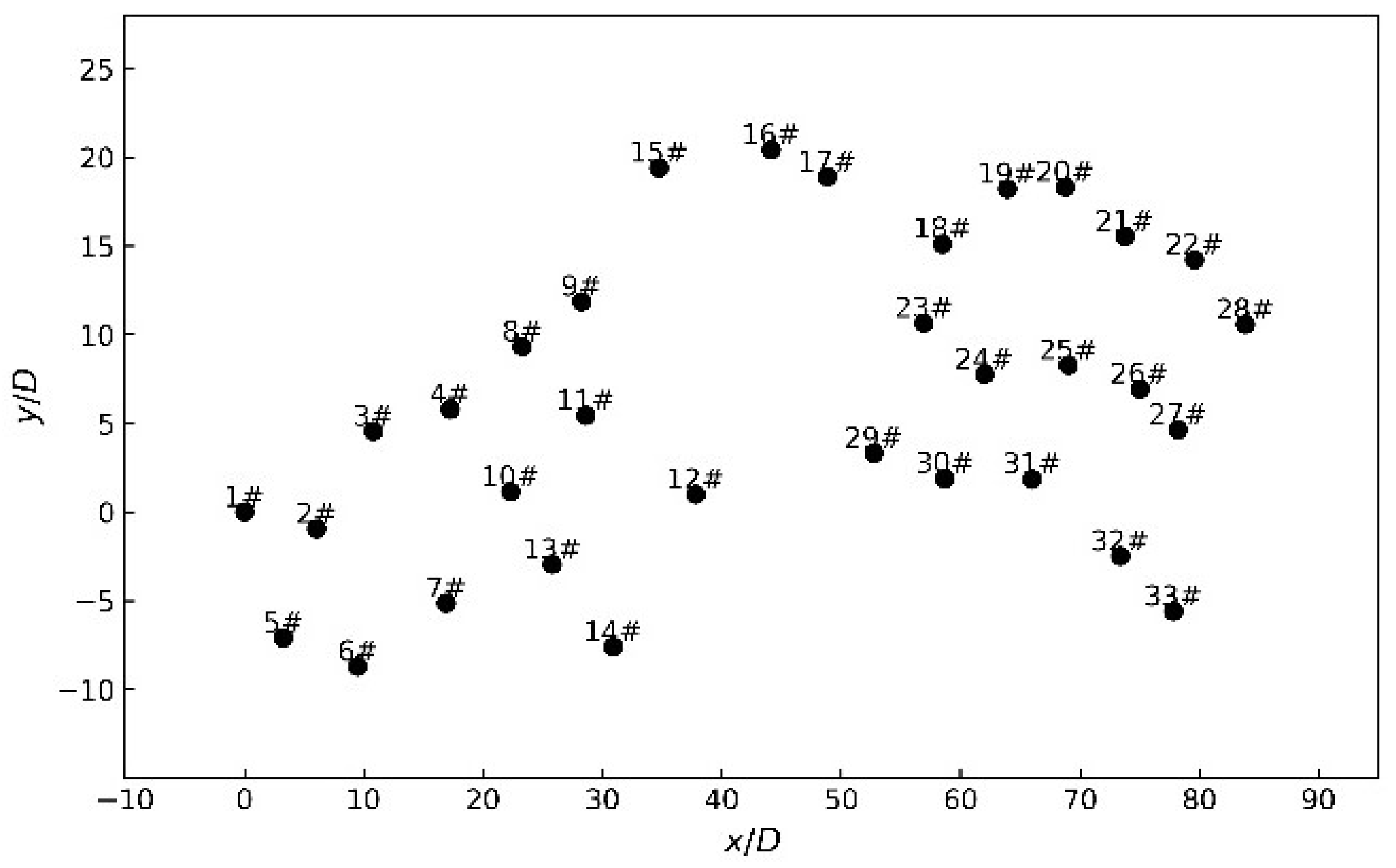
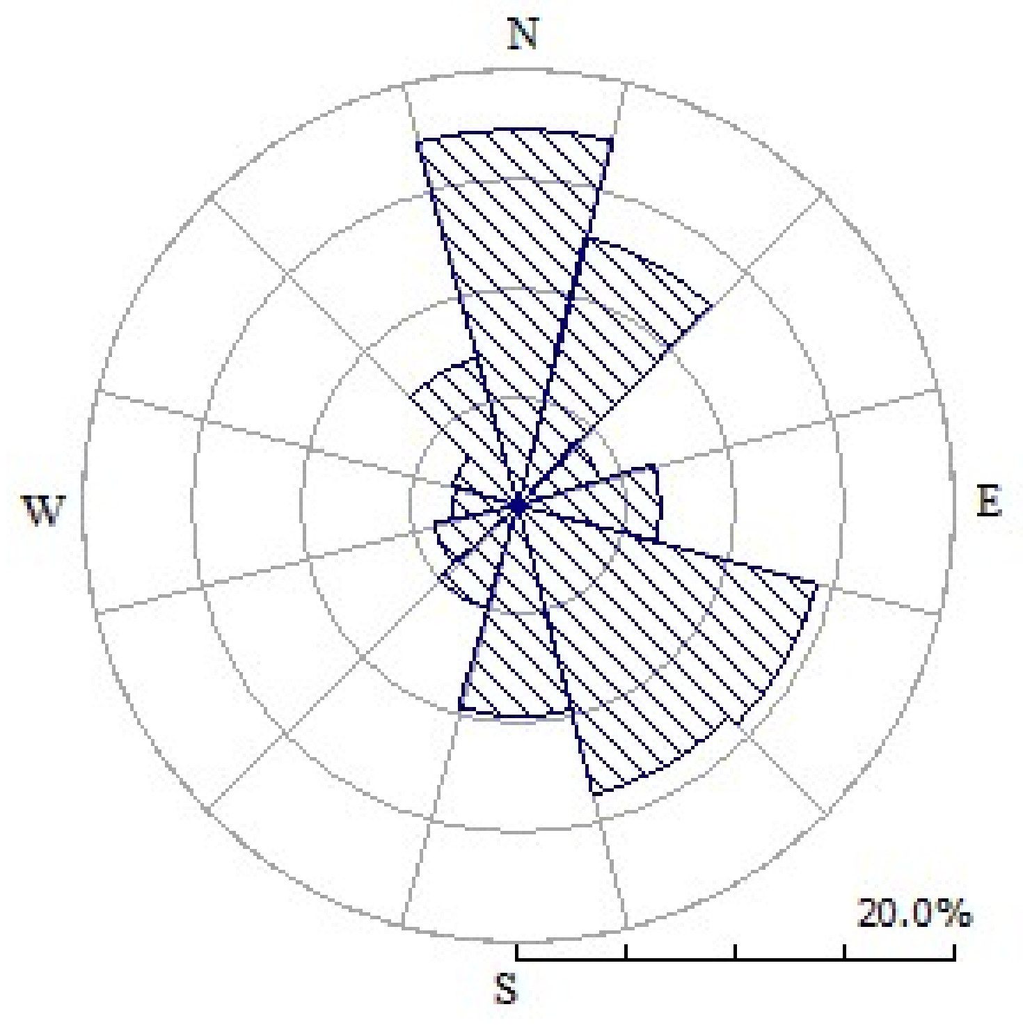
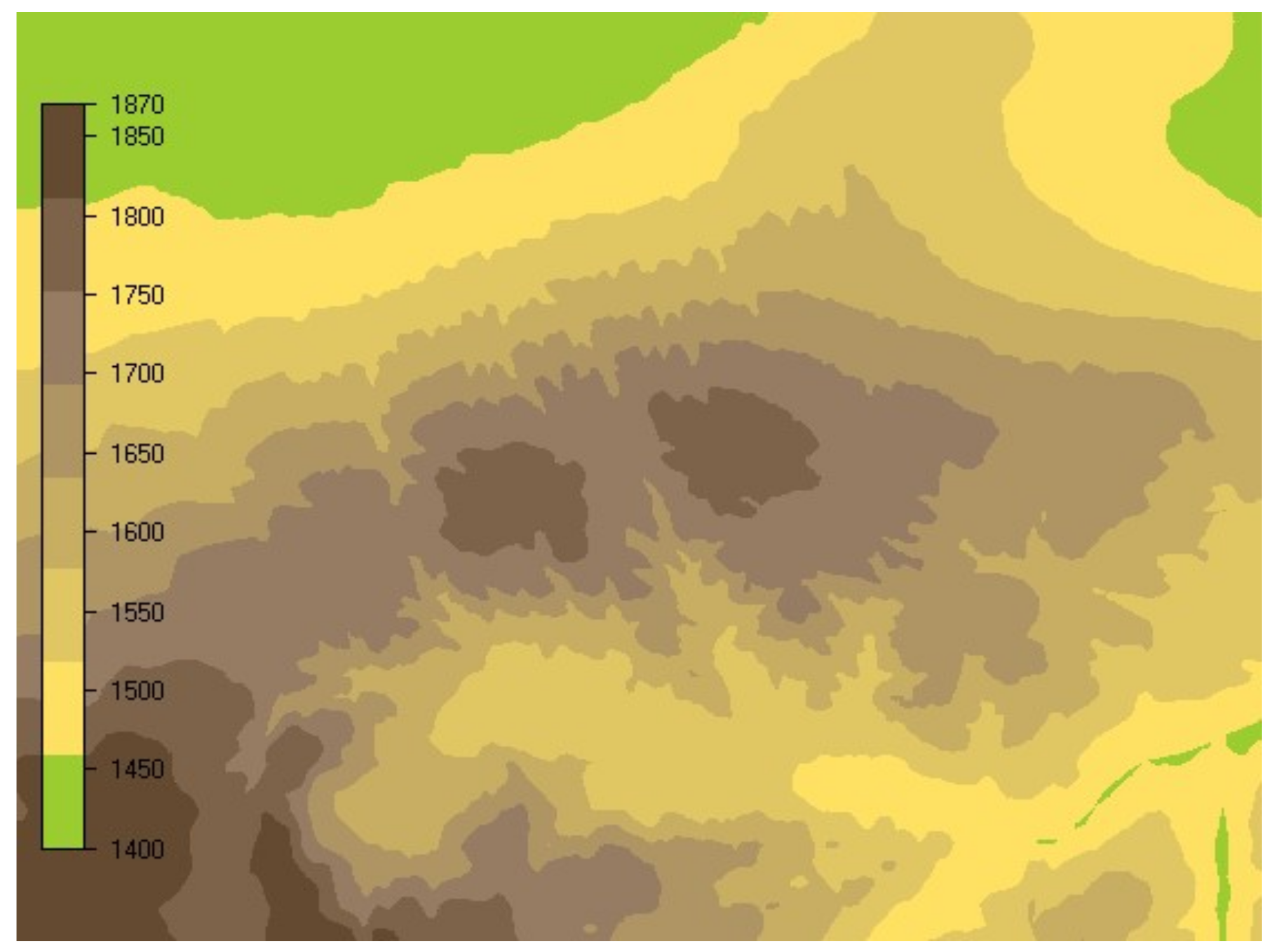
3.1. Wind Farm and Input Data Description

An onshore wind farm in the Shanxi province of northern China is used for wind turbine clustering and subsequent WPF analysis. The wind farm is located in an area of complex terrain, which is the overland of Loess Plateau and desert steppe, and comprises 33 × 1.5 MW wind turbines with the hub heights of 80 m. The maximum elevation difference between turbines is up to 200 m. Figure 1 shows the layout of wind turbines.

The prevailing wind direction at the site is from the north (0° sector), and the corresponding wind rose can be seen in Figure 2. The data obtained from the wind farm include real-time wind speed and output power of each wind turbine for one-year from the supervisory control and data acquisition (SCADA) system on a 15-min basis. Since there is no available NWP, the measured wind speed is used to replace the NWP in this paper. This is not an issue as the aim is to demonstrate the relative improvement in wind power forecasts that can be achieved using clustering.

Due to the effects of wind farm terrain and the wake of upstream wind turbines, wind turbines in different locations experience different wind speeds at hub height and thus, produce different output power. To prepare for WPF, the measured wind power and wind speed of each wind turbine are taken as the inputs to different wind turbine clustering approaches. The characteristics of each wind turbine are represented by four annual average parameters: average wind speed; standard deviation of wind speed; average wind power and standard deviation of wind power. These four parameters respectively for the r-th wind turbine are calculated with Equations (5)–(8):

$$V_{\mathit{mean},r}=\frac{1}{N}{\displaystyle \sum _{i=1}^N{V}_{\mathit{ri}}}$$

(5)

$$V_{\mathit{std},r}=\sqrt{\frac{1}{N}{\displaystyle \sum _{i=1}^N{(V_{\mathit{ri}}-V_{\mathit{mean},r})}^2}}$$

(6)

$$P_{\mathit{mean},r}=\frac{1}{N}{\displaystyle \sum _{i=1}^N{P}_{\mathit{ri}}}$$

(7)

$$P_{\mathit{std},r}=\sqrt{\frac{1}{N}{\displaystyle \sum _{i=1}^N{(P_{\mathit{ri}}-P_{\mathit{mean},r})}^2}}$$

(8)

where V and P are measured wind speed and wind power values, respectively. r = 1, 2, …, m, represents different wind turbines. m is the total number of wind turbines within a wind farm, and N is the size of measured time series (V and P).

The four parameters of each wind turbine are normalized using Equation (9) and form the parameter matrix for the clustering model, which has a size of m × 4:

$$x_{\mathit{norm},r,i}=\frac{x_{r,i}-\mathit{min}(X_i)}{\mathit{max}(X_i)-\mathit{min}(X_i)}$$

(9)

where x_r,i is the ith characteristic value of the rth wind turbine, x_norm,r,i is the normalized value of x_r,i, X_i = {x₁, x₂, …, x_m} is a one-dimensional matrix containing the ith characteristic values of all m wind turbines, i = 1, 2, 3, 4.

3.2. Criteria Used to Assess Clustering Effectiveness

Taking the m × 4 parameter matrix as input, clustering models can be established based on the K-means, HAC and SC algorithms. Analysis of the distance within and between clusters can be undertaken to determine the relative effectiveness of the different clustering approaches. The Silhouette Coefficient, the Calinski-Harabaz and within-between indices have been used in this assessment; they are outlined below.

3.2.1. Silhouette Coefficient

The Silhouette Coefficient (Sico) [39] is used to evaluate the internal cohesion and external separation of clusters. The silhouette value s(x) and Sico are defined in Equations (10) and (11) respectively:

$$s(x)=\frac{b(x)-a(x)}{\mathit{max}\{a(x),b(x)\}}$$

(10)

$$\mathit{Sico}=\frac{1}{m}{\displaystyle \sum _{i=1}^{m}s(x_i)}$$

(11)

where a(x) is the average dissimilarity of x with all the other items within the same cluster, and b(x) is the lowest average dissimilarity of x to any other cluster, of which x is not a member.

s(x) ∈ [−1, 1]. If s(x) ∈ [−1, 0] and b(x) < a(x), the clustering scheme is not reasonable, and least acceptable when s(x) = −1. However, when s(x) ∈ [0, 1] and b(x) > a(x), then the clustering scheme is reasonable, with s(x) = 1 giving the best performance.

3.2.2. Calinski-Harabaz and within-between Indices

The Calinski-Harabaz (CH) index [40] and within-between (WB) index [41] are indices based on the sum of squared distances, and can be computed using Equations (12) and (13), respectively:

$$\mathit{CH}(k)=\frac{\mathit{SSB}/(k-1)}{\mathit{SSW}/(m-k)}$$

(12)

$$\mathit{WB}(k)=k\times \mathit{SSW}/\mathit{SSB}$$

(13)

In the above equations, sum of squares within (SSW) and sum of squares between (SSB) represent the metrics for within cluster variance and between cluster variance, respectively. For a given cluster, SSW is the summation of the squared Euclidean distance between each item within the cluster and the cluster centroid, SSB is the squared Euclidean distance between the cluster centroid and the centroid of all m items times the size of this cluster. The total SSW and SSB of all wind turbines can be calculated from Equations (14) and (15):

$$\mathit{SSW}={{\displaystyle \sum _{i=1}^m\Vert x_i-C_{\mathit{pi}}\Vert }}^2$$

(14)

$$\mathit{SSB}={\displaystyle \sum _{j=1}^k{n}_j}{\Vert C_j-\overline{X}\Vert }^2$$

(15)

where m is the number of wind turbines in a wind farm, k is the number of clusters, C_pi is the cluster center of the pth cluster where the ith wind turbine belongs, n_j is the number of wind turbines in the jth cluster, C_j is the cluster center of the jth cluster, $\overline{X}=\frac{1}{m}{\displaystyle \sum _{i=1}^m{x}_i}$ is the centroid of all wind turbines in the wind farm.

The values of the above three criteria can be used to evaluate different clustering methods and identify the optimal cluster numbers as well, which follow the roles that high values of Sico and CH index indicate effective clustering, whilst a low value of WB index is preferred.

3.3. Wind Turbine Clustering Analysis

K-means, HAC and SC algorithms are used to build wind turbine clustering models within the wind farm and the Sico together with the CH and WB indices are used to evaluate the different cluster models. Finally, the optimal wind turbine clustering scheme for the selected wind farm was determined from the analysis of clustering results. The values of three evaluation indices for the different clustering models has been calculated for cluster number k from two to nine, and then the curves for different indices as a function of cluster number are plotted as in Figure 3.

Figure 3 illustrates that with the increase of cluster number, different clustering methods have similar trends, while the different indices exhibit different trends. The Sico rises to a local maximum at k = 3 for all clustering approaches, then declines to a minimum, and finally increases. The CH index also increases to a maximum at k = 3, and then decreases. The WB index declines rapidly to k = 3 (a local minimum for the HAC) and then in general more slowly with the increasing k. Taking the three measures together suggests that the optimal number of clusters is three for all these three clustering methods. According to Figure 3, for a settled cluster number, K-means model has the highest Sico and CH index values, while with the lowest WB index value as a whole. Thus, for the given case, K-means model gives the overall best clustering results, SC model ranks the second, and HAC performs a little worse than the other two models.

4. Clustering Pre-Calculated CFD-Based WPF

Based on the presented wind turbine clustering models, the CPCC model can be established for short-term WPF. Using the representative wind turbines identified for each cluster, virtual masts can be selected and then applied to the CPCC based WPF.

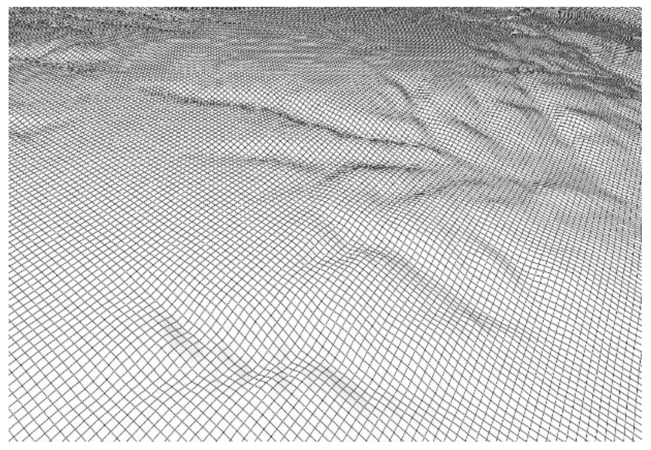
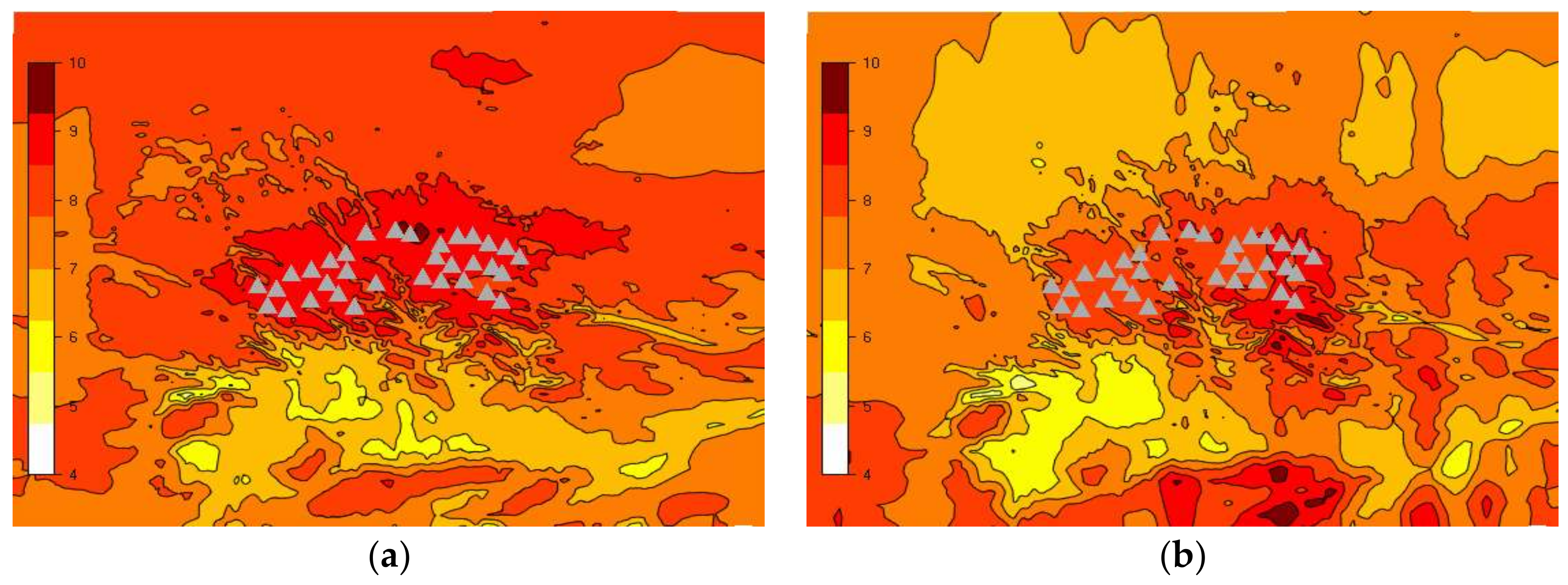
4.1. CFD Database of Flow Field Characteristics

The key point of the CPFF-based WPF method [24,25] is to rescale the predicted meso-scale NWP wind speed from the virtual mast position to every wind turbine location using CFD simulation of wind farm flow fields and so provide wind power forecasts considering both terrain and wake effects. The modeling process can be summarized as follows.

First, a CFD flow model of the wind farm site and surrounding area is constructed (but without wind turbines) based on terrain elevation and surface roughness data. Considering the elevation drop and aspect ratio of the computing domain, the solution domain is specified as an extension of 7 km out of the wind farm boundary in each horizontal direction and about five times the total elevation drop in height direction. Then, a central area refinement meshing scheme is adopted, and the horizontal resolution of the refinement area is 40 m. The elevation distribution and the partial mesh of computation domain showing the changes of topography are shown in Figure 4 and Figure 5. A commercial CFD code PHOENICS with RNG k-ε turbulence model [42] have been used to simulate the wind flow. For each inflow wind condition, the entrance position of the computation domain is determined by the inflow wind direction, and the entrance boundary is set to a vertical wind profile given by the exponential law (Equation (16)). Flow modelling is undertaken for a full range of wind speeds and directions to cover all possible inflow conditions. The inflow wind speeds are respectively set to 2, 4, 6, …, 24 m/s, and the wind directions are distributed in 16 sectors evenly spaced from 0° to 337.5° with the sector width of 22.5°; the combination of each wind speed and each wind direction comprises a discrete inflow, with 192 discrete inflow wind conditions in total. Taking 10 m/s inflow wind speed as an example, the wind velocity distributions of the CFD domain for 0° and 180° inflow wind directions can be obtained and shown in Figure 6:

$$U_n=U_1{\left(\frac{Z_n}{Z_1}\right)}^{\alpha }$$

(16)

where α is the wind shear exponent, Z₁ is the height on the top of the atmospheric boundary layer, U_n and U₁ are the wind velocities at the height Z_n and Z₁, respectively, and U₁ is set to be the speed of inflow wind.

Then the wind turbines and virtual masts are located within the flow domain according to their spatial coordinates, and wake deficits are calculated using the Larsen wake model [43]. The superposition of the wake effects of multiple upstream wind turbines is computed using the sum of squared velocities method [44]. In this manner, the wind speed and direction at each turbine hub height can be obtained. Finally, the wind turbine power curve is used to calculate the output power of the individual wind turbines for all possible wind conditions. These results are formed into a database to be used for the prediction of wind power output.

The Larsen wake model is a fast semi-empirical engineering model used for calculating wind turbine wakes. Assuming the wind velocity deficits of different downstream wind turbines are similar, and then the wake velocity deficit ΔU can be computed using Equation (17):

$$\Delta U=-\frac{U_{\mathit{WT}}}{9}{(C_{T}A{x}^{-2})}^{\frac{1}{3}}{\left[R_w^{\frac{3}{2}}{(3c_1^2{C}_T\mathit{Ax})}^{-\frac{1}{2}}-\left({(\frac{35}{2\pi })}^{\frac{3}{10}}{(3c_1^2)}^{-\frac{1}{3}}\right)\right]}^2$$

(17)

where x is the distance along the axial coordinate direction, A is the swept area of wind rotor, C_T is the thrust coefficient of wind turbine, $c_1$ is the dimensionless mixing length, $U_{\mathit{WT}}$ is the average wind speed at wind turbine hub height, $R_w$ is the wake radius.

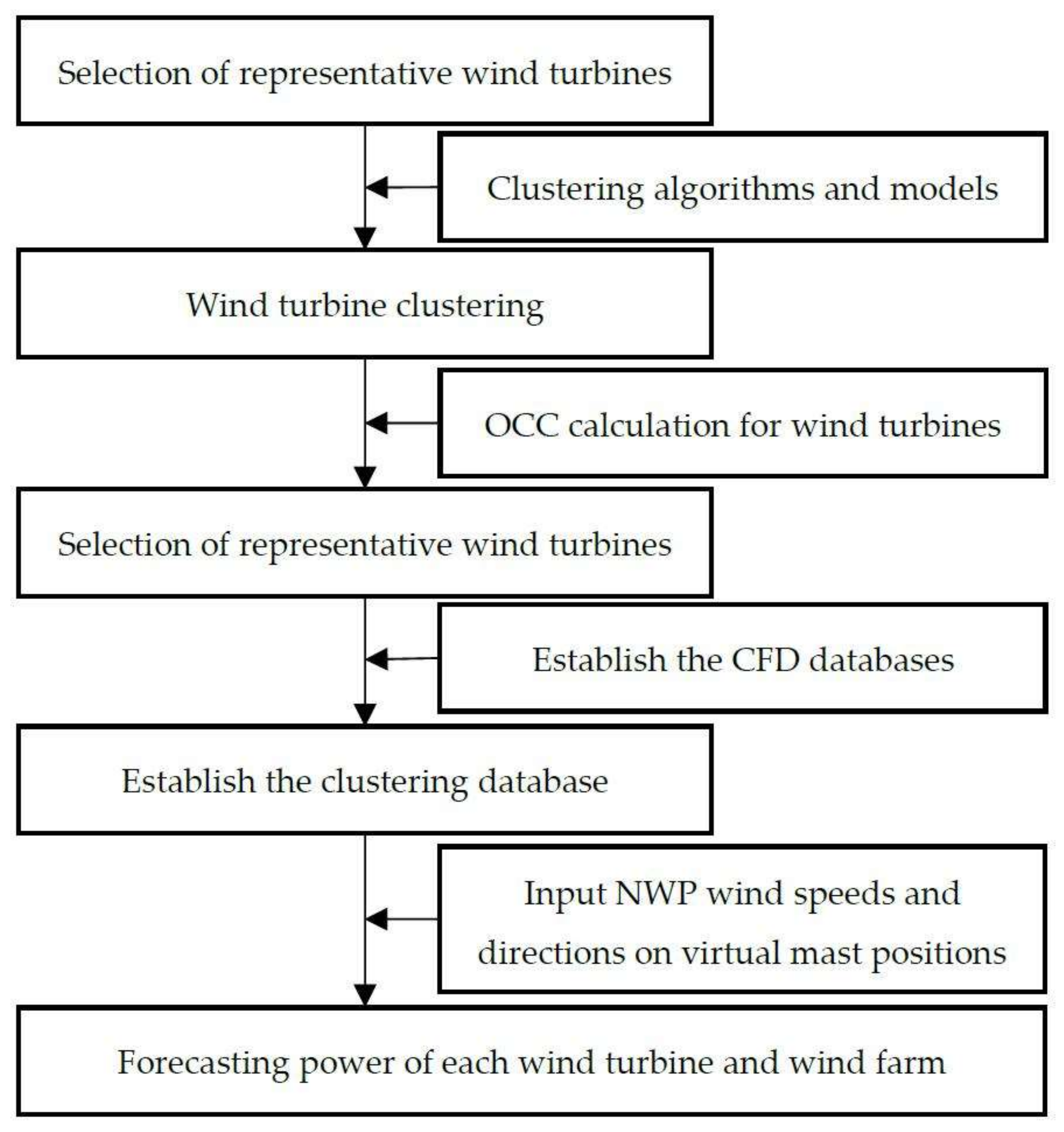
4.2. WPF Model Based on Clustering CFD Database

During the modeling process, the wind turbine that is the most representative of each cluster is selected as the virtual mast, and then the wind speeds at hub height and the output power can be calculated based on the flow fields extrapolated from the virtual mast position. The representative wind turbines can be identified through the calculation of the overall correlation coefficient (OCC) for all wind turbines within each cluster. The turbine with the highest OCC value can be chosen as the representative wind turbine, the OCC is defined according to Equation (18):

$$\mathit{OCC}(X_p)=\frac{1}{m_i}{\displaystyle \sum _{q\in C_i}\frac{\mathit{Cov}(X_p\mathit{,}{X}_q)}{\sqrt{\mathit{Var}(X_p)\mathit{Var}(X_q)}}}$$

(18)

where m_i is the number of the turbines in cluster i, p and q are two arbitrary wind turbines in the ith cluster, p, q ∈ C_i. X_p and X_q are two-dimensional measurement matrixes of the ith and jth wind turbine, respectively. Cov(X_p, X_q) is the covariance between X_p and X_q. Var(X_p) and Var(X_q) are the variance of X_p and X_q, respectively.

Taking the time series data of NWP wind speeds and wind directions at the virtual masts positions as inputs, the corresponding wind power of each wind turbine can be read by searching for neighboring wind conditions in mast columns within each sub-database. Then linear interpolation is used to compute the forecasting output power of every wind turbine under the given input conditions. To take account of wind turbine availability, the predicted power of the whole wind farm is computed from the sum of the forecast power of wind turbines in operation at the time in question. Figure 7 gives the flow chart for establishing a clustering WPF model.

4.3. Case Analysis for Clustering WPF Method

With the flow fields calculated by the CFD model, K-means, HAC and SC methods are applied separately to build the clustering CFD databases for different cluster sizes that can then be used for WPF. According to the stated requirements for short term wind power prediction in China [45], the time resolution should be 15 min, and the monthly root mean square error (RMSE) of short-term WPF should be lower than 20%. RMSE [46] is used as the error index to evaluate the forecasts of wind power for the entire wind farm over one year against measured data:

$$\mathit{RMSE}=\frac{1}{P}\sqrt{\frac{{\displaystyle \sum {(y_t^{\prime }-y_t)}^2}}{N}}$$

(19)

where $y_t^{\prime }$ is the forecast wind power at time t, y_t is the measured wind power at time t, and P is the total capacity of the wind farm.

4.3.1. The Final Clustering Scheme for WPF

For each of these three clustering models considered, the annual RMSE of the predicted wind power for the whole wind farm is calculated while k ranges from two to nine to obtain the curves showing how forecasting error varies with cluster number, as in Figure 8.

Figure 8 illustrates that with the increase of k, the error curves for the three clustering WPF models show similar trends, which initially fall fast and then remain fairly constant. The most consistent minimum error occurs when k is three. Over the range of k from two to nine, the clustering WPF model based on K-means, HAC and SC have the average annual RMSE of 7.5%, 7.8% and 7.6%, respectively.

The HAC method has the highest WPF error, the SC-based model performs a little better, and K-means clustering method shows the best WPF accuracy. The error analysis above confirms the conclusions drawn from the assessment of clustering performance presented in Section 3.3, which in turn proves the effectiveness of the three indices (Sico, CH and WB) used in clustering assessments.

The optimal cluster number for all three methods is found to be three. Moreover, all three clustering models produce exactly the same clustering scheme for k is three. According to the OCC computations for all wind turbines, the optimal clustering scheme and the corresponding OCCs of all wind turbines are shown in

Table 1. The optimal clustering scheme and OCC statistics of all wind turbines. (k = 3).

Cluster I		Cluster II		Cluster III
WT	OCC (%)	WT	OCC (%)	WT	OCC (%)
2	89.30	6	90.52	1	92.11
4	90.58	7	93.38	3	91.92
5	89.86	10	93.37	8	93.55
9	91.62	11	89.46	15	93.77
18	92.63	12	93.83	16	91.53
21	87.50	13	93.84	17	90.14
22	91.99	14	92.83	19	92.39
23	92.81	24	91.59	20	92.02
25	92.59	27	91.01
26	92.84	29	90.50
28	91.64	30	93.73
		31	93.69
		32	92.78
		33	92.68

. Grey highlights show the highest OCC values of each cluster.

Table 1 indicates that the numbers of wind turbines in the three clusters are 11, 14 and 8, respectively. The wind turbines that have the highest OCCs within each cluster are 26#, 13# and 15#, respectively. These three representative wind turbine locations are taken as the virtual masts of three sub-databases used for WPF.

4.3.2. WPF Analysis for Optimal Clustering Scheme

Based on the consistent assessments of clustering performance and WPF accuracy, the optimal clustering with k = 3 is used to establish CFD flow field databases. By taking the NWP time series data of wind speed and wind direction at the location of 13#, 15# and 26# turbines as input, respectively, and then searching for nearby wind conditions in the established databases, the power generated by the wind turbines within each cluster can be calculated by linear interpolation. Compared with the measurement data of the wind farm, RMSE is taken as error index to evaluate the improvements from the optimal clustering WPF model against the WPF models without clustering for different spatial and temporal scales.

(1) Annual error of forecasting wind power

The annual RMSEs of the wind power predicted by both the clustering database and three sub-databases for the entire wind farm are presented in Figure 9, and for every wind turbine individually in Figure 10.

As can be seen from Figure 9 and Figure 10, compared with all sub-databases, the clustering database gives the highest annual accuracy for both individual wind turbines and whole wind farm. For the whole wind farm, the use of the clustering database helps to reduce the error by 4.2%, 5.2% and 2.9% for 13#, 15# and 26# databases, respectively. For the annual RMSE of a single wind turbine, the clustering database has the same error as each sub-database for the wind turbines within the corresponding cluster.

(2) Monthly error of forecasting wind power

Based on the clustering database and sub-databases, the monthly RMSE of the forecasting wind power for the entire farm can be computed and plotted as Figure 11.

As can be seen in Figure 11, the 15# database has the highest annual and monthly RMSE, and 26# database has the lowest ones. For all these databases, the RMSEs of June and October are much higher than the other months. The clustering database has managed to decrease the RMSE of June by 4.0%, 8.4% and 3.2% respectively for three sub-databases, and the RMSE of October has been decreased by 6.0%, 4.7% and 2.8%, respectively. For the wind power predicted by clustering database, the monthly RMSE of twelve months are all lower than 10%.

(3) Error distributions for forecasting wind power

It is also instructive to investigate the error distributions for the forecasting power associated with different databases. 5% is used as the error interval and then errors within [−50%, +50%] are presented. The mid-point of each interval is employed to represent each 5% wide interval as in Figure 12.

From Figure 12, it is clear that using clustering by far the highest proportion, 49.8%, falls into the zero error category [−2.5%, +2.5%], which is significantly higher than 38.2%, 39.7% and 42.0% for three sub-databases. Over 90% of the cluster based forecasting power fall into the range of −10% to 10%.

(4) Short-term wind power forecasts

Whether for the whole year or 12 individual months, for the whole wind farm or 33 individual wind turbines, the clustering database always gives better accuracy than the other three sub-databases. Figure 13 shows the comparisons between predicted and measured wind power for short-term trends over three days from two selected months (January and April).

It is apparent that the power predicted by sub-databases reasonably follows the general variational trends of measured wind power. However, for the time points where there is an abrupt change of the output wind power (or wind speed), the predicted wind power can deviate markedly from the measured one. In contrast, the use of clustering significantly improves the accuracy in this situation.

5. Conclusions

In this paper, three indices to evaluate clustering effectiveness have been used to assess the performance of the different proposed clustering methods. The clustering models presented in this paper were then applied to CPCC based WPF. From the error analysis of wind power forecasts, the following conclusions can be drawn.

(1)

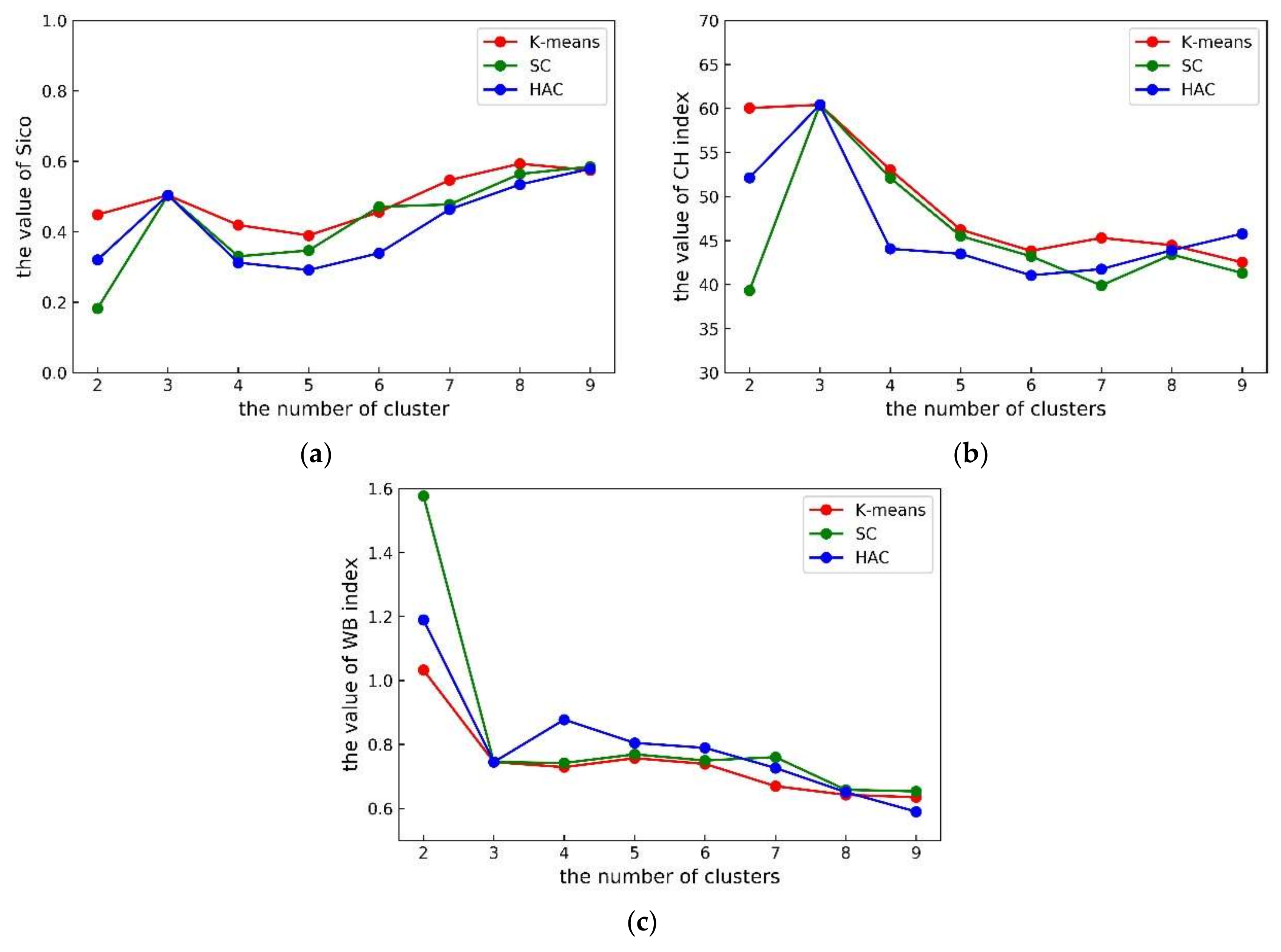
The analysis of WPF error confirmed the effectiveness of the three measures (Silhouette Coefficient, Calinski-Harabaz and WB indices) for assessing clustering performance proposed in this paper, and the three clustering evaluation indices are all in close agreement.

(2)

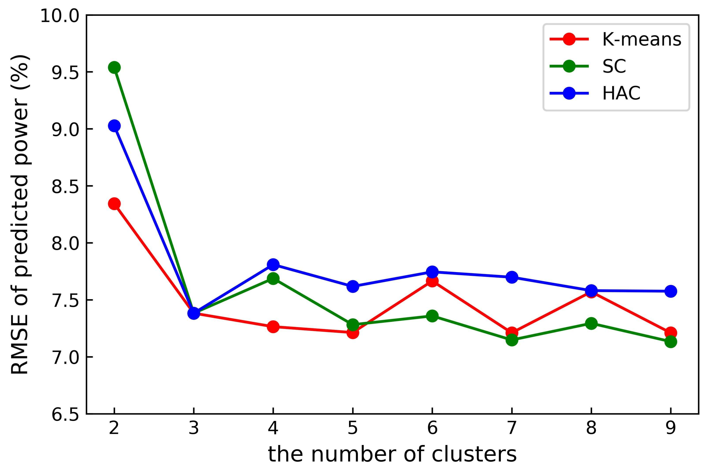
For a given cluster number k, K-means method gives the best clustering results, SC ranks the second, and HAC is a little worse than the other two methods. For k is three, all three clustering methods give the same clustering performance, in fact they share exact the same clustering scheme.

(3)

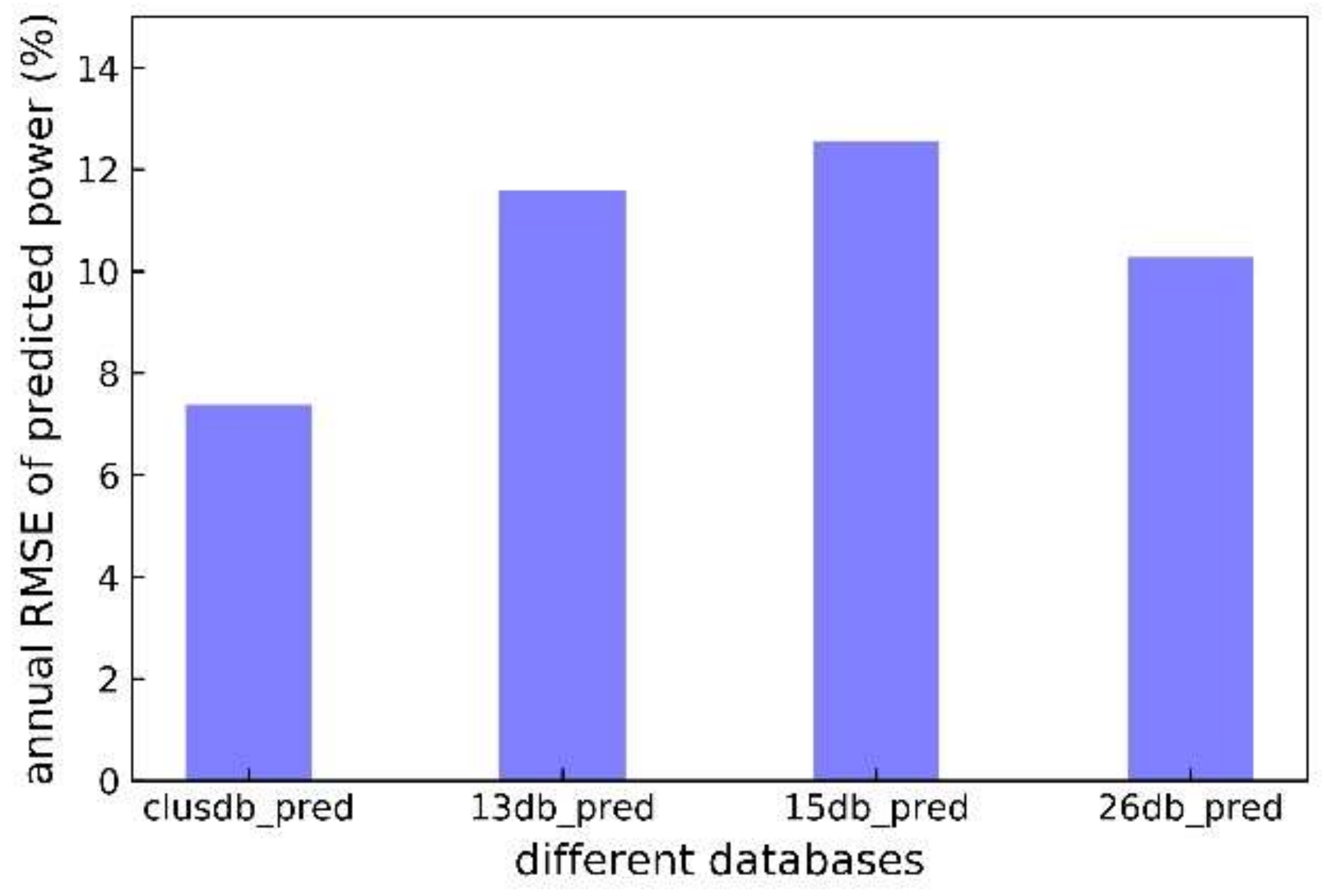
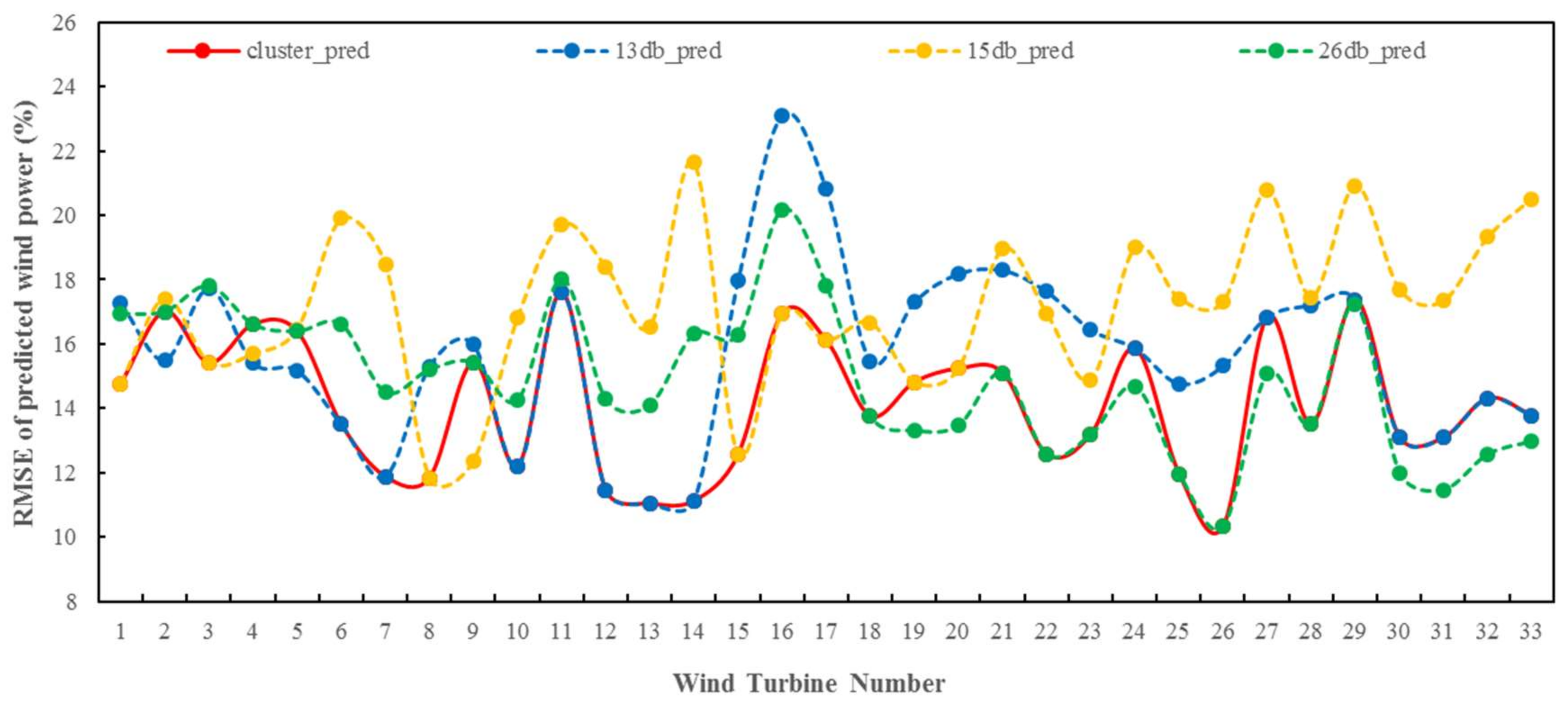
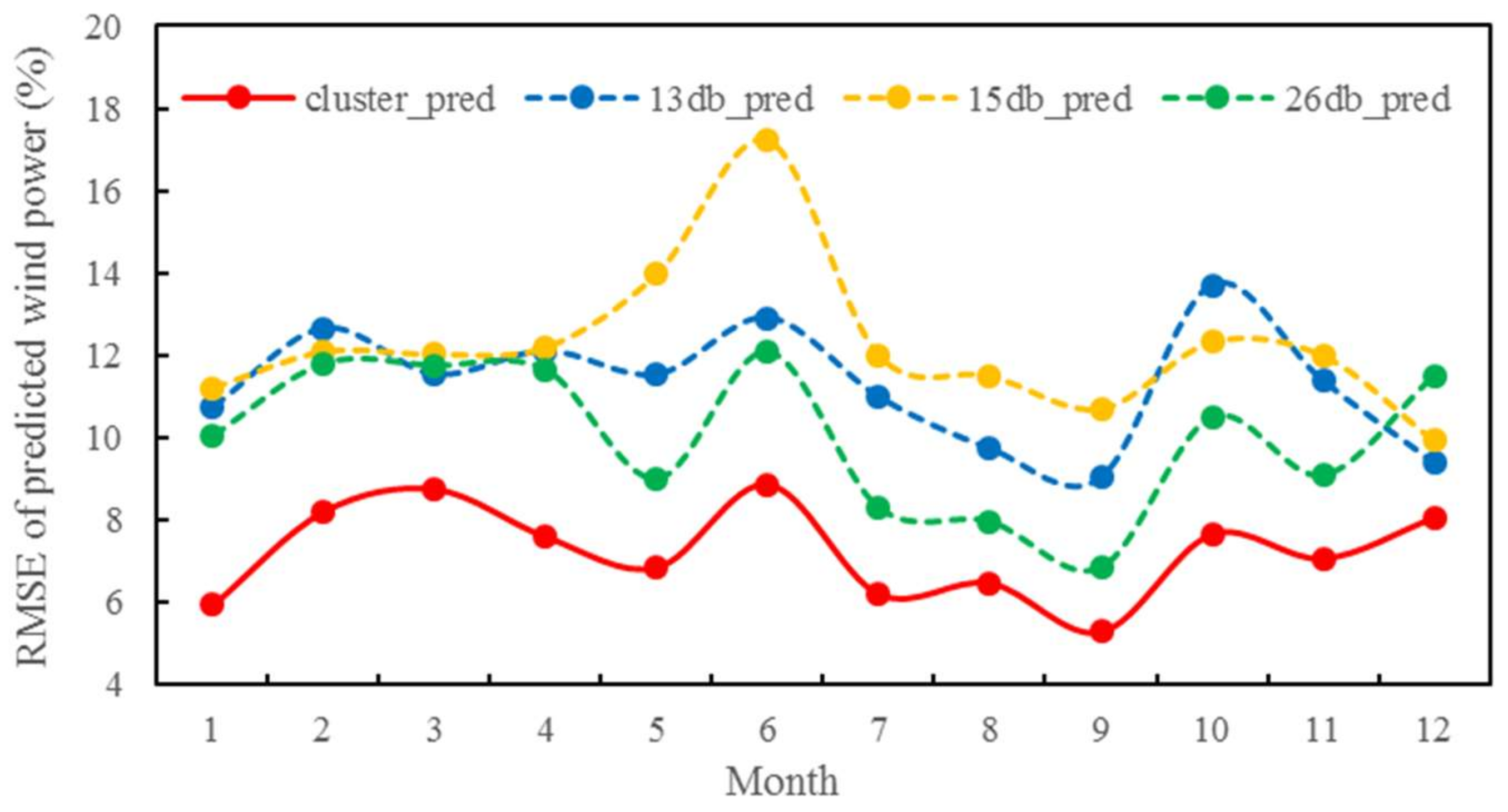
For different temporal scales (yearly, monthly or daily) and spatial scales (wind farm or wind turbine), the clustering approach always produces more accurate forecasts power than those from single sub-databases, and can decrease the annual forecasting RMSE of the whole wind farm by up to 5.2%.

(4)

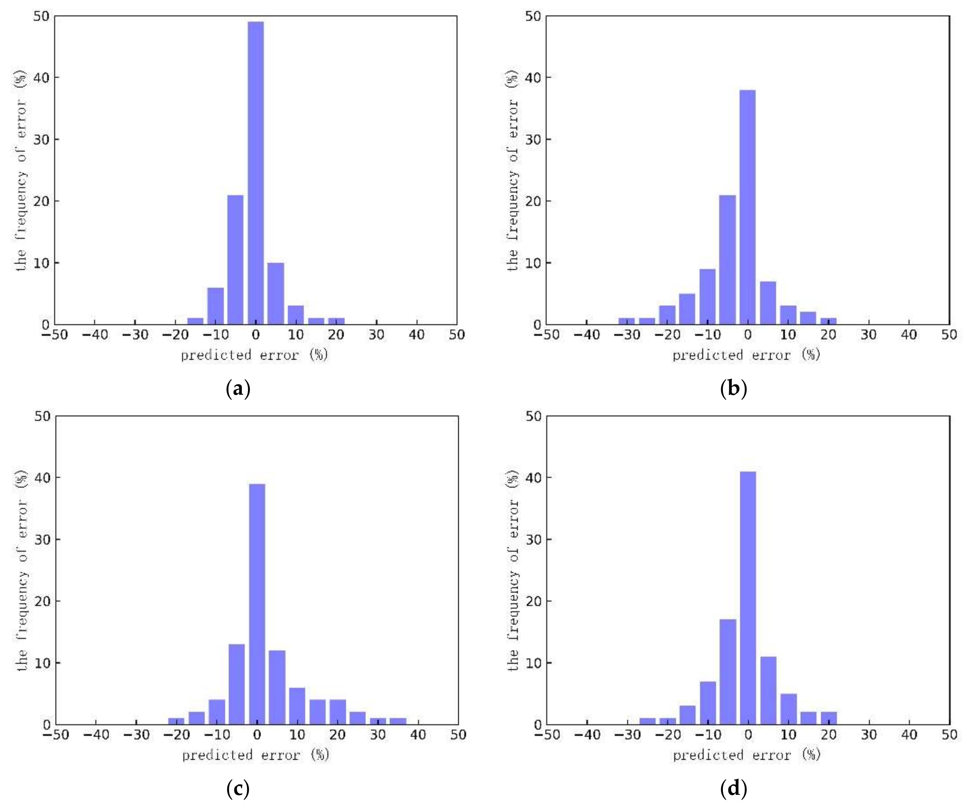
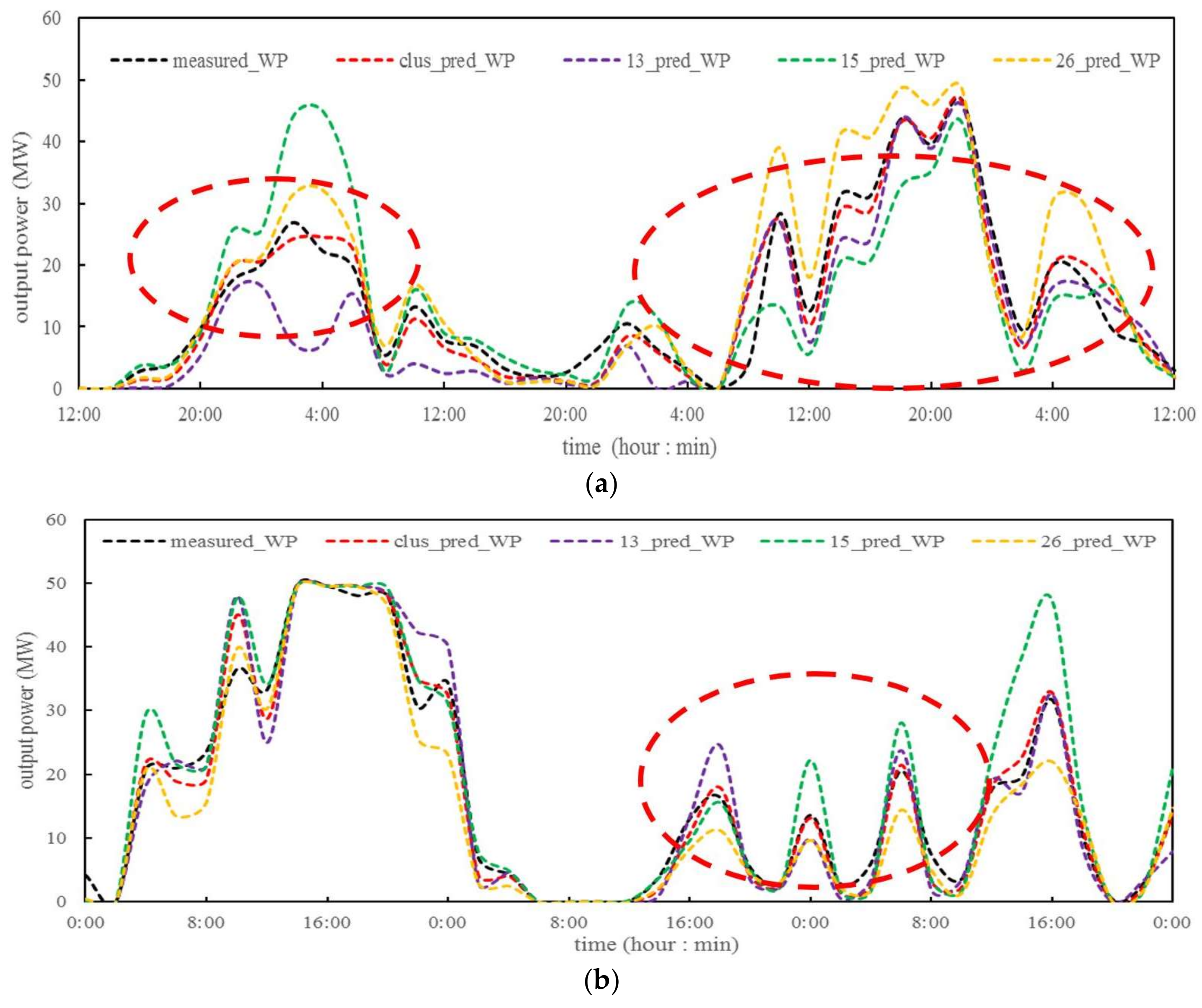
Use of clustering database dramatically improves the distribution of forecasting errors. The errors within [−10%, 10%] are 14.4% higher than 15# sub-database. The clustering database produces more accurate wind power predictions for different short-term variation scenarios than the other sub-databases.

References

1. Lauha, F.; Limig, Q.; Steve, S.; Sgruti, S. Global Wind Report Annual Market Update 2016; Global Wind Energy Council: Brussels, Belgium, 2017. [Google Scholar]
2. Lu, X.; McElroy, M.B.; Peng, W.; Liu, S.; Nielsen, C.P.; Wang, H. Challenges faced by China compared with the US in developing wind power. Nat. Energy 2016, 1, 16061. [Google Scholar] [CrossRef]
3. Zhang, X.; Ma, C.; Song, X.; Zhou, Y.; Chen, W. The impacts of wind technology advancement on future global energy. Appl. Energy 2016, 184, 1033–1037. [Google Scholar] [CrossRef]
4. Lund, H. Large-scale integration of wind power into different energy systems. Energy 2005, 30, 2402–2412. [Google Scholar] [CrossRef]
5. Lei, M.; Shiyan, L.; Chuanwen, J.; Hongling, L.; Yan, Z. A review on the forecasting of wind speed and generated power. Renew. Sustain. Energy Rev. 2009, 13, 915–920. [Google Scholar] [CrossRef]
6. Ren, G.; Liu, J.; Wan, J.; Guo, Y.; Yu, D. Overview of wind power intermittency: Impacts, measurements, and mitigation solutions. Appl. Energy 2017, 204, 47–65. [Google Scholar] [CrossRef]
7. Jung, J.; Broadwater, R.P. Current status and future advances for wind speed and power forecasting. Renew. Sustain. Energy Rev. 2014, 31, 762–777. [Google Scholar] [CrossRef]
8. Colak, I.; Sagiroglu, S.; Yesilbudak, M. Data mining and wind power prediction: A literature review. Renew. Energy 2012, 46, 241–247. [Google Scholar] [CrossRef]
9. Wang, H.-Z.; Li, G.-Q.; Wang, G.-B.; Peng, J.-C.; Jiang, H.; Liu, Y.-T. Deep learning based ensemble approach for probabilistic wind power forecasting. Appl. Energy 2017, 188, 56–70. [Google Scholar] [CrossRef]
10. Shuang-Lei, F.; Wei-Sheng, W.; Chun, L.; Hui-zhu, D. Study on the physical approach to wind power prediction. Proc. CSEE 2010, 30, 1–6. [Google Scholar]
11. Al-Yahyai, S.; Charabi, Y.; Gastli, A. Review of the use of Numerical Weather Prediction (NWP) Models for wind energy assessment. Renew. Sustain. Energy Rev. 2010, 14, 3192–3198. [Google Scholar] [CrossRef]
12. Lange, M.; Focken, U. Physical Approach to Short-Term Wind Power Prediction; Springer: New York, NY, USA, 2006. [Google Scholar]
13. Landberg, L. Short-term prediction of the power production from wind farms. J. Wind Eng. Ind. Aerodyn. 1999, 80, 207–220. [Google Scholar] [CrossRef]
14. Ye, L.; Zhao, Y.; Zeng, C.; Zhang, C. Short-term wind power prediction based on spatial model. Renew. Energy 2017, 101, 1067–1074. [Google Scholar] [CrossRef]
15. Marjanovic, N.; Wharton, S.; Chow, F.K. Investigation of model parameters for high-resolution wind energy forecasting: Case studies over simple and complex terrain. J. Wind Eng. Ind. Aerodyn. 2014, 134, 10–24. [Google Scholar] [CrossRef]
16. Murali, A.; Rajagopalan, R. Numerical simulation of multiple interacting wind turbines on a complex terrain. J. Wind Eng. Ind. Aerodyn. 2017, 162, 57–72. [Google Scholar] [CrossRef]
17. Politis, E.S.; Prospathopoulos, J.; Cabezon, D.; Hansen, K.S.; Chaviaropoulos, P.; Barthelmie, R.J. Modeling wake effects in large wind farms in complex terrain: The problem, the methods and the issues. Wind Energy 2012, 15, 161–182. [Google Scholar] [CrossRef] [Green Version]
18. Carvalho, D.; Rocha, A.; Santos, C.S.; Pereira, R. Wind resource modelling in complex terrain using different mesoscale–microscale coupling techniques. Appl. Energy 2013, 108, 493–504. [Google Scholar] [CrossRef]
19. Castellani, F.; Vignaroli, A. An application of the actuator disc model for wind turbine wakes calculations. Appl. Energy 2013, 101, 432–440. [Google Scholar] [CrossRef]
20. Castellani, F.; Astolfi, D.; Mana, M.; Piccioni, E.; Becchetti, M.; Terzi, L. Investigation of terrain and wake effects on the performance of wind farms in complex terrain using numerical and experimental data. Wind Energy 2017, 20, 1277–1289. [Google Scholar]
21. Göçmen, T.; Van der Laan, P.; Réthoré, P.-E.; Diaz, A.P.; Larsen, G.C.; Ott, S. Wind turbine wake models developed at the technical university of Denmark: A review. Renew. Sustain. Energy Rev. 2016, 60, 752–769. [Google Scholar] [CrossRef] [Green Version]
22. Sanderse, B. Aerodynamics of Wind Turbine Wakes; ECN-E–09-016; Energy Research Center of the Netherlands (ECN): Petten, The Netherlands, 2009; Volume 5, p. 153. [Google Scholar]
23. Castellani, F.; Astolfi, D.; Mana, M.; Burlando, M.; Meißner, C.; Piccioni, E. Wind Power Forecasting techniques in complex terrain: ANN vs. ANN-CFD hybrid approach. J. Phys. Conf. Ser. 2016, 753, 082002. [Google Scholar] [CrossRef]
24. Li, L.; Liu, Y.; Yang, Y.; Han, S. Short-term wind speed forecasting based on CFD pre-calculated flow fields. Proc. CSEE 2013, 33, 27–32. [Google Scholar]
25. Li, L.; Liu, Y.-Q.; Yang, Y.-P.; Shuang, H.; Wang, Y.-M. A physical approach of the short-term wind power prediction based on CFD pre-calculated flow fields. J. Hydrodyn. Ser. B 2013, 25, 56–61. [Google Scholar] [CrossRef]
26. Liu, Y.; Wang, Y.; Li, L.; Han, S.; Infield, D. Numerical weather prediction wind correction methods and its impact on computational fluid dynamics based wind power forecasting. J. Renew. Sustain. Energy 2016, 8, 033302. [Google Scholar] [CrossRef] [Green Version]
27. Lin, L.; Chen, Y.; Wang, N. Clustering wind turbines for a large wind farm using spectral clustering approach based on diffusion mapping theory. In Proceedings of the 2012 IEEE International Conference on Power System Technology (POWERCON), Auckland, New Zealand, 30 October–2 November 2012; pp. 1–6. [Google Scholar]
28. Fahad, A.; Alshatri, N.; Tari, Z.; Alamri, A.; Khalil, I.; Zomaya, A.Y.; Foufou, S.; Bouras, A. A survey of clustering algorithms for big data: Taxonomy and empirical analysis. IEEE Trans. Emerg. Top. Comput. 2014, 2, 267–279. [Google Scholar] [CrossRef]
29. Yan, J.; Liu, Y.; Han, S.; Qiu, M. Wind power grouping forecasts and its uncertainty analysis using optimized relevance vector machine. Renew. Sustain. Energy Rev. 2013, 27, 613–621. [Google Scholar] [CrossRef]
30. Liu, D.; Wang, J.; Wang, H. Short-term wind speed forecasting based on spectral clustering and optimised echo state networks. Renew. Energy 2015, 78, 599–608. [Google Scholar] [CrossRef]
31. Dong, L.; Wang, L.; Khahro, S.F.; Gao, S.; Liao, X. Wind power day-ahead prediction with cluster analysis of NWP. Renew. Sustain. Energy Rev. 2016, 60, 1206–1212. [Google Scholar] [CrossRef]
32. Li, S.; Ma, H.; Li, W. Typical solar radiation year construction using k-means clustering and discrete-time Markov chain. Appl. Energy 2017, 205, 720–731. [Google Scholar] [CrossRef]
33. Kanungo, T.; Mount, D.M.; Netanyahu, N.S.; Piatko, C.D.; Silverman, R.; Wu, A.Y. An efficient k-means clustering algorithm: Analysis and implementation. IEEE Trans. Pattern Anal. Mach. Intell. 2002, 24, 881–892. [Google Scholar] [CrossRef]
34. Zepeda-Mendoza, M.L.; Resendis-Antonio, O. Hierarchical agglomerative clustering. In Encyclopedia of Systems Biology; Springer: New York, NY, USA, 2013; pp. 886–887. [Google Scholar]
35. Day, W.H.; Edelsbrunner, H. Efficient algorithms for agglomerative hierarchical clustering methods. J. Classif. 1984, 1, 7–24. [Google Scholar] [CrossRef]
36. Ding, C.; He, X. Cluster merging and splitting in hierarchical clustering algorithms. In Proceedings of the Data Mining, Maebashi City, Japan, 9–12 December 2002; pp. 139–146. [Google Scholar]
37. Von Luxburg, U. A tutorial on spectral clustering. Stat. Comput. 2007, 17, 395–416. [Google Scholar] [CrossRef]
38. Ng, A.Y.; Jordan, M.I.; Weiss, Y. On spectral clustering: Analysis and an algorithm. Proc Nips 2001, 14, 849–856. [Google Scholar]
39. Rousseeuw, P.J. Silhouettes: A graphical aid to the interpretation and validation of cluster analysis. J. Comput. Appl. Math. 1987, 20, 53–65. [Google Scholar] [CrossRef]
40. Caliński, T.; Harabasz, J. A dendrite method for cluster analysis. Commun. Stat. Theory Methods 1974, 3, 1–27. [Google Scholar] [CrossRef]
41. Zhao, Q.; Fränti, P. WB-index: A sum-of-squares based index for cluster validity. Data Knowl. Eng. 2014, 92, 77–89. [Google Scholar] [CrossRef]
42. Yakhot, V.; Orszag, S.A. Renormalization group analysis of turbulence. I. Basic theory. J. Sci. Comput. 1986, 1, 3–51. [Google Scholar] [CrossRef]
43. Larsen, G.C. A Simple Stationary Semi-Analytical Wake Model; Risø National Laboratory for Sustainable Energy, Technical University of Denmark: Roskilde, Denmark, 2009. [Google Scholar]
44. Kuo, J.Y.; Romero, D.A.; Amon, C.H. A mechanistic semi-empirical wake interaction model for wind farm layout optimization. Energy 2015, 93, 2157–2165. [Google Scholar] [CrossRef]
45. Liu, C.; Pei, Z.Y.; Wang, B.; Dong, C.; Feng, S.L.; Fan, G.F.; Shi, Y.G.; Fan, G.Y.; Guo, L. Function Specification of Wind Power Forecasting; China Electric Power Press: Beijing, China, 2011. [Google Scholar]
46. Ouyang, T.; Zha, X.; Qin, L. A combined multivariate model for wind power prediction. Energy Convers. Manag. 2017, 144, 361–373. [Google Scholar] [CrossRef]
Figure 1. Layout of wind turbines.
Energies 11 00854 g001
Figure 2. Wind rose.
Energies 11 00854 g002
Figure 3. The variation of indices with the increase of cluster number for the different models: (a) Silhouette coefficient; (b) Calinski-Harabaz index; (c) WB index.
Energies 11 00854 g003
Figure 4. Elevation distribution within wind farm area.
Energies 11 00854 g004
Figure 5. Partial mesh in computational domain.
Energies 11 00854 g005
Figure 6. Velocity field distributions under different inflow wind directions (unit: m/s): (a) North wind; (b) South wind.
Energies 11 00854 g006
Figure 7. The modeling process of the WPF based on clustering database.
Energies 11 00854 g007
Figure 8. The annual RMSEs of different clustering WPF models as a function of cluster number.
Energies 11 00854 g008
Figure 9. The annual RMSE of wind farm output power predicted by different databases.
Energies 11 00854 g009
Figure 10. The annual RMSE of wind turbine output power predicted by different databases.
Energies 11 00854 g010
Figure 11. The monthly RMSE of the power predicted by different databases.
Energies 11 00854 g011
Figure 12. Error frequency distributions for different databases: (a) clustering database; (b) 13# sub-database; (c) 15# sub-database; (d) 26# sub-database.
Energies 11 00854 g012
Figure 13. Short-term variations of the predicted power using different databases: (a) January; (b) April.
Energies 11 00854 g013