A Distributed Robust Dispatch Approach for Interconnected Systems with a High Proportion of Wind Power Penetration

Abstract

This paper proposes a distributed robust dispatch approach to solve the economic dispatch problem of the interconnected systems with a high proportion of wind power penetration. First of all, the basic principle of synchronous alternating direction method of multipliers (SADMM) is introduced to solve the economic dispatch problem of the two interconnected regions. Next, the polyhedron set of the robust optimization method is utilized to describe the wind power output. To adjust the conservativeness of the polyhedron set, an adjustment factor of robust conservativeness is introduced. Subsequently, considering the operation characteristics of the DC tie line between the interconnected regions, an economic dispatch model with a high proportion of wind power penetration is established and parallel iteration based on SADMM is used to solve the model. In each iteration, the optimized power of DC tie lines is exchanged between the regions without requiring the participation of the superior dispatch center. Finally, the validity of the proposed model is verified by the examples of the 2-area 6-node interconnected system and the interconnection of several modified New England 39-node systems. The results show that the proposed model can meet the needs of the independent dispatch of regional power grids, effectively deal with the uncertainty of wind power output, and maximize the wind power consumption under the condition of ensuring the safe operation of the interconnected systems.

1. Introduction

With the penetration of a high proportion of wind power, as well as the rapid development of power grid, great challenges have emerged in the economic dispatch of the power system. On the one hand, wind power output is featured by volatility and anti-peak. Therefore, how to deal with the impact of wind power penetration on the economic dispatch of the power system is a valuable topic that deserves further study [1,2,3,4]. On the other hand, the links between regional power grids are getting closer and closer through the ultrahigh voltage (UHV) DC transmission, and meanwhile the requirements for the communication capabilities of power grids are getting higher and higher accordingly. Thus, how to achieve the optimal dispatch of the whole power system under the precondition of reducing the computing scale of the interconnected system has become a research hotspot nowadays [5,6,7,8].

During the process of dealing with the uncertainties of wind power output, literature [9] proposes a dispatch method using energy storage to deal with the forecasting error of wind power, which aims to minimize the sum of the investment cost, operation cost, and load-shedding cost. A probability distribution model is put forward by literature [10] to describe the forecasting error of wind power, and then it is applied to the economic dispatch of the wind power system. Furthermore, literature [11] proposes a two-stage power generation model and solves the problem using stochastic programming by introducing demand response to make wind power output smoother. In literature [12], a robust optimization method is employed to describe the wind power output. The literature also establishes a day-ahead dispatch model that aims to minimize the total cost under the worst scenario and introduces adjustable parameters to control the conservativeness of the model. Literature [13] adopts both stochastic programming and fuzzy programming to describe the wind power output and utilizes the particle swarm algorithm to solve the established two-stage, multi-objective dispatch model. Although the above literatures provide some methods to deal with the uncertainties of wind power output, they are all limited to the centralized dispatch of a single region and fail to take into account the current status of China’s regional power grid interconnection.

As for the distributed optimization [14,15] of the power system, literature [16] solves the AC-DC security-constrained unit commitment (SCUC) problem by using a convex relaxation technique and introduces the conditional value-at risk to limit the risk of deviations in the load demand and renewable generation. Literature [17] proposes a decentralized decision-making algorithm based on analytical target cascading (ATC) for optimization in complex systems. Literature [18] proposes a self-decision method of load management based on multi-agent systems, in which the upstream grid, distributed generation, and demand response resources are taken into consideration. Literature [19] proposes a centralized approach for the independent system operator to solve a direct current optimal power flow (DCOPF) problem based on demand response. The lagrangian relaxation method is utilized in literature [20] to decompose the economic dispatch problem of the interconnected power system into the independent sub-problems. However, the introduction of a large number of Lagrange multipliers will lead to the reduction of the convergence of the solution. Literature [21] applies the augmented Lagrangian relaxation method in the multi-region economic dispatch, yet the problem of indivisibility of the algorithm needs to be solved by the principle of the auxiliary problem. In literature [22], a modified generalized Benders decomposition method is adopted to address the multi-region dynamic economic dispatch problem with wind power penetration. However, a reasonable correction constraint needs to be introduced into each iteration. Literature [23,24] solves the problem of economic dispatch in the multi-region interconnected power system dispersedly with the usage of the target cascade method. However, it is necessary to construct an upper coordinator to achieve inter-region coordination and optimization. In literature [25], the optimal condition decomposition method is adopted to decompose the optimal power flow problem in the interconnected regions, yet the operation characteristics of the tie lines are considered in a rough way. As an essential method in the field of decentralized optimization, an alternating direction method of multipliers (ADMM) has some advantages in the rate of convergence [26,27,28,29]. However, the coordination and optimization of the upper coordinator are needed during the iteration. Compared with the above methods, SADMM not only has the characteristics of sound convergence performance but also does not require the participation of the upper coordinator in the process of problem solving. Therefore, it solves the problem more quickly.

The contributions of this paper are as follows: (1) The polyhedron set in robust optimization is adopted to describe wind power output, and an adjustment factor of robust conservativeness is introduced to adjust the conservativeness of problem solving. (2) The decentralized robust dispatch model with a high proportion of wind power penetration is established. (3) The SADMM algorithm is utilized to solve the established model. In the process of optimization, each region is independently responsible for the optimal dispatch problem in the region and does not need the participation of the superior dispatch center. The model is addressed in parallel and the optimized power of each DC tie line is exchanged between regions after each iteration. (4) Examples are given to verify the validity of the proposed model.

The rest of the paper is organized as follows. The second part describes the basic principle of SADMM. The third part is the establishment of the decentralized economic dispatch model. The solving process of the model and case study are provided in the fourth part. The fifth part is the conclusions of the full text.

2. Basic Principle of SADMM

Taking the two-region interconnected system as an example, the standard alternating direction method of multipliers (ADMM) is presented as follows:

$$\{\begin{array}{l}\min F_1(x_1)+F_2(x_2)\\ \mathrm{s}.\mathrm{t}.\mathit{A}{x}_1=\mathit{B}{x}_2\end{array}$$

(1)

When ADMM is used to address the problem, the updated iterative equation is as follows:

$$\{\begin{array}{l}{x}_1^{k+1}=\arg \min [F_1(x_1^k)+{({\mathit{\lambda }}^k)}^{\mathrm{T}}(\mathit{A}{x}_1^k-\mathit{B}{x}_2^k)+\frac{\beta }{2}{\Vert \mathit{A}{x}_1^k-\mathit{B}{x}_2^k\Vert }^2]\\ x_2^{k+1}=\arg \min [F_2(x_2^k)+{({\mathit{\lambda }}^k)}^{\mathrm{T}}(\mathit{A}{x}_1^{k+1}-\mathit{B}{x}_2^k)+\frac{\beta }{2}{\Vert \mathit{A}{x}_1^{k+1}-\mathit{B}{x}_2^k\Vert }^2]\\ {\mathit{\lambda }}^{k+1}={\mathit{\lambda }}^k+\beta (\mathit{A}{x}_1^{k+1}-\mathit{B}{x}_2^{k+1})\end{array}$$

(2)

According to the ADMM iteration process, the principle is a serial iteration. That is, the latter region needs to make use of the optimization value of the previous region when optimizing the solution. When all the regions are optimized, the Lagrange multiplier is updated by the upper coordinator and then distributed to the dispersed regions. Obviously, this iteration is slow and is not conducive to the large-scale calculations. Therefore, some work has been done to convert ADMM to SADMM. Parallel iteration is utilized in SADMM without the participation of the upper coordinator in the process of problem solving, so the speed of problem solving is faster than ADMM. The following is the process of conversion from ADMM to SADMM.

In the first line of Equation (2), the latter two of augmented Lagrangian functions can be expressed as

$${({\mathit{\lambda }}^k)}^{\mathrm{T}}(\mathit{A}{x}_1^k-\mathit{B}{x}_2^k)+\frac{\beta }{2}{\Vert \mathit{A}{x}_1^k-\mathit{B}{x}_2^k\Vert }^2=\frac{\beta }{2}{\Vert \mathit{A}{x}_1^k-\mathit{B}{x}_2^k+\frac{1}{\beta }{\mathit{\lambda }}^k\Vert }^2-\frac{1}{2\beta }{\Vert {\mathit{\lambda }}^k\Vert }^2$$

(3)

Let ${\mathit{\nu }}^k$ = $\frac{1}{\beta }{\mathit{\lambda }}^k$; if the constant term $\frac{1}{2\beta }{\Vert {\mathit{\lambda }}^k\Vert }^2$ is omitted, then Equation (2) can be converted into

$$\{\begin{array}{l}{x}_1^{k+1}=\arg \min \left[F_1(x_1^k)+\frac{\beta }{2}{\Vert \mathit{A}{x}_1^k-\mathit{B}{x}_2^k+{\mathit{\nu }}^k\Vert }^2\right]\\ x_2^{k+1}=\arg \min \left[F_2(x_2^k)+\frac{\beta }{2}{\Vert \mathit{A}{x}_1^{k+1}-\mathit{B}{x}_2^k+{\mathit{\nu }}^k\Vert }^2\right]\\ {\mathit{\nu }}^{k+1}={\mathit{\nu }}^k+(\mathit{A}{x}_1^{k+1}-\mathit{B}{x}_2^{k+1})\end{array}$$

(4)

Take the average of each optimization result of two regions, and let

$${\overline{x}}_1^k={\overline{x}}_2^k=\frac{(\mathit{A}{x}_1^k+\mathit{B}{x}_2^k)}{2}$$

(5)

Then, let Equation (5) replace the optimization result of the adjacent regions to be selected next in Equation (4), that is, if one lets ${\overline{x}}_1^k$ replace $\mathit{B}{x}_2^k$ and ${\overline{x}}_2^k$ replace $\mathit{A}{x}_1^{k+1}$, the expression of SADMM can be obtained:

$$\{\begin{array}{l}{x}_1^{k+1}=\arg \min \left[F_1(x_1^k)+\frac{\beta }{2}{\Vert \mathit{A}{x}_1^k-{\overline{x}}_1^k+{\mathit{\nu }}_1^k\Vert }^2\right]\\ {\mathit{\nu }}_1^{k+1}={\mathit{\nu }}_1^k+(\mathit{A}{x}_1^{k+1}-{\overline{x}}_1^{k+1})\end{array}$$

(6)

$$\{\begin{array}{l}{x}_2^{k+1}=\arg \min \left[F_2(x_2^k)+\frac{\beta }{2}{\Vert {\overline{x}}_2^k-\mathit{B}{x}_2^k+{\mathit{\nu }}_2^k\Vert }^2\right]\\ {\mathit{\nu }}_2^{k+1}={\mathit{\nu }}_2^k+({\overline{x}}_2^{k+1}-\mathit{B}{x}_2^{k+1})\end{array}$$

(7)

The basic principle of solving the economic dispatch problem of the two interconnected regions using SADMM is as follows. First of all, the interconnected regions are decomposed into two independently operated regions, and then the two regions are optimized using parallel computing. The calculation result of each iteration needs to be exchanged between the regions. The average value of the optimization result of the two regions is taken as the optimization result of the adjacent regions to be selected in the next iteration. The entire process does not need the participation of the upper coordinator, which can not only reduce the computing scale of the interconnected regions but also achieve decentralized control.

3. Decentralized Economic Dispatch Model of the Interconnected Power System

The schematic diagram of interconnected power system is shown in Figure 1; taking region A as an example, the corresponding optimization dispatch model is established based on the SADMM algorithm as follows.

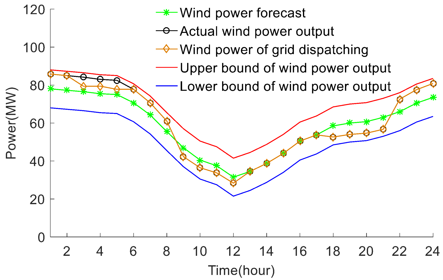
3.1. Modeling of Wind Power Output

In this paper, a robust optimization method is utilized to describe the wind power output. Suppose region A contains $M$ wind farms with a total of $T$ dispatch time intervals, the output of wind farm $j$ in the time period $t$ is $P_{j,t}^{\mathrm{W}}$, which is an uncertain parameter for the dispatch. Its output forecast value is $P_{j,t}^{\mathrm{e}}$. First of all, according to the weather forecast information, the predicted interval of wind power output can be obtained as follows:

$$P_{j,t}^{\mathrm{Wmin}}\le P_{j,t}^{\mathrm{W}}\le P_{j,t}^{\mathrm{Wmax}}$$

(8)

Considering the space cluster effect, restriction on the overall deviation of all wind power output prediction in each dispatch time interval $t$ is added

$${\displaystyle {\sum }_j\left|P_{j,t}^{\mathrm{W}}-P_{j,t}^{\mathrm{e}}\right|}/P_{j,t}^{\mathrm{Wh}}\le {\Gamma }^{\mathrm{S}}$$

(9)

in which

$$P_{j,t}^{\mathrm{e}}=\frac{\left(P_{j,t}^{\mathrm{Wmax}}+P_{j,t}^{\mathrm{Wmin}}\right)}{2}$$

(10)

$$P_{j,t}^{\mathrm{Wh}}=\frac{\left(P_{j,t}^{\mathrm{Wmax}}-P_{j,t}^{\mathrm{Wmin}}\right)}{2}$$

(11)

Similarly, taking into account the time smoothed effect, the limit of the overall deviation of all wind power output predictions in all periods is added to a particular wind farm $j$.

$${\displaystyle {\sum }_t\left|P_{j,t}^{\mathrm{W}}-P_{j,t}^{\mathrm{e}}\right|}/P_{j,t}^{\mathrm{Wh}}\le {\Gamma }^{\mathrm{T}}$$

(12)

To sum up, the set of wind power output $P^{\mathrm{W}}$ can be described as follows:

$$P^{\mathrm{W}}=\left\{P_{j,t}^{\mathrm{W}}|\begin{array}{l}{P}_{j,t}^{\mathrm{Wmin}}\le P_{j,t}^{\mathrm{W}}\le P_{j,t}^{\mathrm{Wmax}}\\ {\displaystyle {\sum }_j\left|P_{j,t}^{\mathrm{W}}-P_{j,t}^{\mathrm{e}}\right|}/P_{j,t}^{\mathrm{Wh}}\le {\Gamma }^{\mathrm{S}}\\ {\displaystyle {\sum }_t\left|P_{j,t}^{\mathrm{W}}-P_{j,t}^{\mathrm{e}}\right|}/P_{j,t}^{\mathrm{Wh}}\le {\Gamma }^{\mathrm{T}}\end{array}\right\}$$

(13)

Here, literature [30] describes the uncertainty that is used, and the set described by Equation (13) can be expressed as follows:

$$P^{\mathrm{W}}=\left\{P_{j,t}^{\mathrm{W}}|\begin{array}{l}{P}_{j,t}^{\mathrm{W}}=P_{j,t}^{\mathrm{e}}+P_{j,t}^{\mathrm{Wh}}{\tau }_{j,t},\left|{\tau }_{j,t}\right|\le 1\\ {\displaystyle \sum _{j=1}^M\left|{\tau }_{j,t}\right|\le {\Gamma }^{\mathrm{S}},{\displaystyle \sum _{t=1}^T\left|{\tau }_{j,t}\right|\le {\Gamma }^{\mathrm{T}}}}\end{array}\right\}$$

(14)

The parameters ${\Gamma }^{\mathrm{S}}$ and ${\Gamma }^{\mathrm{T}}$ are utilized to control the severity of the uncertainty, and they also reflect the risk appetite of policymakers.

If ${\Gamma }^{\mathrm{S}}$ and ${\Gamma }^{\mathrm{T}}$ are integers, the set expressed by Equation (14) has a single-mode matrix structure. Under the most uncertain circumstances, the below equation appears:

$${\displaystyle \sum _{j=1}^M\left|{\tau }_{j,t}\right|={\Gamma }^{\mathrm{S}},{\displaystyle \sum _{t=1}^T\left|{\tau }_{j,t}\right|={\Gamma }^{\mathrm{T}}}}$$

(15)

In this case, since the set represented by Equation (14) is a polyhedron, the worst case of the uncertainty it imposes must occur on the pole [31]. Thus, only the pole set of the polyhedron needs to be taken into consideration. It has the following representation:

$$P^{\mathrm{W}}=\left\{P_{j,t}^{\mathrm{W}}|\begin{array}{ccc}\hfill P_{j,t}^{\mathrm{W}}& =& P_{j,t}^{\mathrm{e}}+\left({\tau }_{j,t}^{+}-{\tau }_{j,t}^{-}\right)P_{j,t}^{\mathrm{Wh}}\hfill \\ \hfill \mathrm{s}.\mathrm{t}.& & {\tau }_{j,t}^{+}+{\tau }_{j,t}^{-}\le 1,{\tau }_{j,t}^{+},{\tau }_{j,t}^{-}\in \left\{0,1\right\}\hfill \\ & & {\displaystyle \sum _{j=1}^M\left({\tau }_{j,t}^{+}+{\tau }_{j,t}^{-}\right)\le {\Gamma }^{\mathrm{S}}}\hfill \\ & & {\displaystyle \sum _{t=1}^T\left({\tau }_{j,t}^{+}+{\tau }_{j,t}^{-}\right)\le {\Gamma }^{\mathrm{T}}}\hfill \end{array}\right\}$$

(16)

Equation (16) is equivalent to Equation (13) in the worst case of uncertainty. However, the conservativeness of the wind power output set expressed by Equation (16) is high. Therefore, to reduce the conservativeness of the problem, adjustable parameters are introduced in the set that describes the wind power output, and the rest of the constraints remain unchanged. The specific form is shown as follows:

$$P_{j,t}^{\mathrm{W}}=P_{j,t}^{\mathrm{e}}+\lambda \left({\tau }_{j,t}^{+}-{\tau }_{j,t}^{-}\right)P_{j,t}^{\mathrm{Wh}}$$

(17)

The range of $\lambda$ is $0\le \lambda \le 1$. It is adopted to adjust the conservativeness of the robust optimization problem so that the wind power output will not reach the boundary in the worst case.

3.2. The Objective Function

The optimization goals of region A include thermal power generation cost, wind power abandonment cost, and deviation penalty cost of tie line power. In fact, the aim of adding the deviation penalty cost of the tie line power is to make the optimization results of region A and region B become closer so as to achieve the optimization of the entire interconnected power system. The concrete form of the objective function is as follows:

$$\min {\displaystyle \sum _{t\in T}\left\{{\displaystyle \sum _{i\in N_{\mathrm{G}}^{\mathrm{A}}}{F}_i(P_{i,t}^{\mathrm{G}})}+{\displaystyle \sum _{j\in N_{\mathrm{W}}^{\mathrm{A}}}{C}_{\mathrm{W}}\Delta P_{j,t}^{\mathrm{W}}}+\frac{\beta }{2}{\Vert P_{m,t}^{\mathrm{dc}}-{\overline{P}}_t^{\mathrm{dc}}+P_{f,t}^{\mathrm{dc}}\Vert }^2\right\}}$$

(18)

in which

$$F_i(P_{i,t}^{\mathrm{G}})=a_i{(P_{i,t}^{\mathrm{G}})}^2+b_i(P_{i,t}^{\mathrm{G}})+c_i$$

(19)

$$\Delta P_{j,t}^{\mathrm{W}}=P_{j,t}^{\mathrm{W}}-P_{j,t}^{\mathrm{WS}}$$

(20)

3.3. The Constraints

For the optimal dispatch model of the wind power system, the constraints usually include:

$${\displaystyle \sum _{i\in N_{\mathrm{G}}^{\mathrm{A}}}{P}_{i,t}^{\mathrm{G}}+{\displaystyle \sum _{j\in N_{\mathrm{W}}^{\mathrm{A}}}{P}_{j,t}^{\mathrm{WS}}-P_{m,t}^{\mathrm{dc}}=}}{\displaystyle \sum _{k\in {\mathsf{\Phi }}_{\mathrm{D}}^{\mathrm{A}}}{P}_{k,t}^{\mathrm{D}}}$$

(21)

$$P_{i,t}^{\mathrm{Gmin}}\le P_{i,t}^{\mathrm{G}}\le P_{i,t}^{\mathrm{Gmax}}$$

(22)

$$R_i^{\mathrm{G}-}\le P_{i,t}^{\mathrm{G}}-P_{i,t-1}^{\mathrm{G}}\le R_i^{\mathrm{G}+}$$

(23)

$$\{\begin{array}{l}{\displaystyle \sum _{i=1}^{N_{\mathrm{G}}^{\mathrm{A}}}\min (P_{i,t}^{\mathrm{Gmax}}-P_{i,t}^{\mathrm{G}},r_i^{\mathrm{u}}{T}_0)\ge R_{\mathrm{A},t}^{+}+{\overline{P}}_{mn}^{\mathrm{dc}}}\\ R_{\mathrm{A},t}^{+}={\omega }_{\mathrm{D}}{\displaystyle \sum _{k\in {\mathsf{\Phi }}_{\mathrm{D}}^{\mathrm{A}}}{P}_{k,t}^{\mathrm{D}}}+{\omega }_{\mathrm{u}}{\displaystyle \sum _{j\in N_{\mathrm{W}}^{\mathrm{A}}}{\overline{P}}_{j,t}^{\mathrm{W}}}\end{array}$$

(24)

$$\{\begin{array}{l}{\displaystyle \sum _{i=1}^{N_{\mathrm{G}}^{\mathrm{A}}}\min (P_{i,t}^{\mathrm{G}}-P_{i,t}^{\mathrm{Gmin}},r_i^{\mathrm{d}}{T}_0)\ge R_{\mathrm{A},t}^{-}-{\underset{\_}{P}}_{mn}^{\mathrm{dc}}}\\ R_{\mathrm{A},t}^{-}={\omega }_{\mathrm{d}}{\displaystyle \sum _{j\in N_{\mathrm{W}}^{\mathrm{A}}}{P}_{j,t}^{\mathrm{W}}}\end{array}$$

(25)

$$|{\displaystyle \sum _{i\in N_{\mathrm{G}}^{\mathrm{A}}}{S}_{li}^{\mathrm{G}}{P}_{i,t}^{\mathrm{G}}+{\displaystyle \sum _{j\in N_{\mathrm{W}}^{\mathrm{A}}}{S}_{lj}^{\mathrm{W}}{P}_{j,t}^{\mathrm{WS}}}}-S_{lm}^{\mathrm{dc}}{P}_{m,t}^{\mathrm{dc}}-{\displaystyle \sum _{k\in {\mathsf{\Phi }}_{\mathrm{D}}^{\mathrm{A}}}{S}_{lk}^{\mathrm{D}}{P}_{k,t}^{\mathrm{D}}}|\le {\overline{F}}_l$$

(26)

$$0\le P_{j,t}^{\mathrm{WS}}\le P_{j,t}^{\mathrm{W}}$$

(27)

Equations (21)–(27) are separately powered balance constraint, thermal power output constraint, climbing constraint, positive spinning reserve constraint, negative spinning reserve constraint, power flow safety constraint, and wind power output constraint.

For the DC tie lines between the interconnected regions, the constraints that the output needs to satisfy are as follows:

$$P_t^{\min ,\mathrm{dc}}\le P_{m,t}^{\mathrm{dc}}\le P_t^{\max ,\mathrm{dc}}$$

(28)

$$\left(x_t^{+}+x_t^{-}\right){\underset{\_}{\Delta }}_t^{\mathrm{dc}}\le \left|P_{t+1}^{\mathrm{dc}}-P_t^{\mathrm{dc}}\right|\le \left(x_t^{+}+x_t^{-}\right){\overline{\Delta }}_t^{\mathrm{dc}}$$

(29)

$$\{\begin{array}{l}{x}_t^{+}+x_{t+1}^{-}\le 1\\ x_t^{-}+x_{t+1}^{+}\le 1\end{array}$$

(30)

$$\{\begin{array}{l}{x}_t^{+}+x_{t+1}^{+}\le 1\\ x_t^{-}+x_{t+1}^{-}\le 1\end{array}$$

(31)

$$x_t^{+}+x_t^{-}\le 1$$

(32)

$${\displaystyle \sum _{t\in T}\left(x_t^{+}+x_t^{-}\right)}\le N_{\max }$$

(33)

$${\displaystyle \underset{1}{\overset{T}{\int }}{P}_t^{\mathrm{dc}}·\Delta t\mathrm{d}t}=Q$$

(34)

Equations (28)–(34) separately represent the output constraint of the DC tie lines, the constraint of the adjustment rate of the output, the constraint of not being adjusted in different directions in the adjacent periods, the constraint of not being adjusted continuously in the adjacent periods, the constraint of climbing and landslide not being performed at the same time, the constraint of output adjustment times, and the constraint of the total amount of electricity delivered within the planning period.

4. Model Solving and Case Study

4.1. Integrated Schematic of the Whole Study

The integrated schematic of the whole study is described as follows:

Step 1:

Input the predicted load demand, predicted wind power output, and initial transmission plan.

Step 2:

Propose a distributed robust dispatch model to solve the economic dispatch problem of the interconnected power system with a high proportion of wind power penetration.

Step 3:

Solve the model by using the SADMM algorithm.

Step 4:

Solve the hybrid integer quadratic programming problem on the Matlab2016a platform.

Step 5:

Output and analyze the simulation results.

This process can be described by the flow chart shown in Figure 2.

4.2. Flow Chart of Model Solving Based on the SADMM

Based on the basic principle of the SADMM algorithm, the convergence condition of the model solution in the iterative process is as follows:

$$\left|P_{m,t}^{\mathrm{dc}}(k)-P_{n,t}^{\mathrm{dc}}(k)\right|\le \mathsf{\epsilon }$$

(35)

If the convergence condition is not satisfied in the $k$ iteration, ${\overline{P}}_t^{\mathrm{dc}}$ and $P_{f,t}^{\mathrm{dc}}$ are updated according to Equations (36) and (37), and then the next iteration is performed.

$${\overline{P}}_t^{\mathrm{dc}}(k+1)=\frac{P_{m,t}^{\mathrm{dc}}(k)+P_{n,t}^{\mathrm{dc}}(k)}{2}$$

(36)

$$P_{f,t+1}^{\mathrm{dc}}(k+1)=P_{f,t}^{\mathrm{dc}}(k)+P_{m,t+1}^{\mathrm{dc}}(k)-{\overline{P}}_t^{\mathrm{dc}}(k+1)$$

(37)

Based on the SADMM algorithm, the solution flow chart of the decentralized economic dispatch model with a high proportion of wind power penetration is presented in Figure 3.

4.3. Case Study

The hybrid integer quadratic programming problem is the essence of the solution of the distributed economic dispatch model with a high proportion of wind power penetration established in the paper. Yalmip programming is adopted on the Matlab2016a (2016a, MathWorks, Natick, MA, USA) platform and Gurobi solver is selected to address this problem. The CPU in the testing environment is a Quad-core processor with 8 GB memory. The two examples are selected to verify the validity of the model.

4.3.1. A 2-Area 6-Node System

First of all, a 2-area 6-node interconnected system is utilized to simulate the interconnection of the grids of both region A and region B. The regions are connected by a DC tie line. Additionally, the interconnected system includes a wind farm, which is located at node 2 in region A. The structure is presented in Figure 4, and the relevant parameters of the thermal power units are shown in

Table 1. Conventional unit parameters.

Generator	${\mathit{P}}_{\mathit{i},\mathit{t}}^{\mathbf{Gmin}}$ (MW)	${\mathit{P}}_{\mathit{i},\mathit{t}}^{\mathbf{Gmax}}$ (MW)	${\mathit{a}}_{\mathit{i}}$ ($/h)	${\mathit{b}}_{\mathit{i}}$ ($/MW·h)	${\mathit{c}}_{\mathit{i}}$ ($/MW·h2)
G1	10	100	100	30	0.3
G2	10	75	100	40	0.8
G3	10	50	100	20	0.2
G4	10	100	200	60	0.6
G5	10	75	200	80	1.6
G6	10	50	200	40	0.4

. To make the power exchange between the regions more obvious, the coal consumption factor of region B relative to region A is considered as 1.5, the demand coefficient of the load for the positive spinning reserve is ${\omega }_D$ = 10%, the demand coefficient of the wind power for the positive and negative spinning reserves is ${\omega }_u$ = ${\omega }_d$ = 10%, the upper limit of the transmission of the DC tie line is 50 MW, the convergence precision of the SADMM algorithm is $\mathsf{\epsilon }$ = 10⁻⁵, the robust conservativeness factor is $\lambda$ = 0.5, and the forecast value of wind power and load is presented in Figure 5. Additionally, Figure 6 shows the initial transmission plan of the DC tie line.

Based on the SADMM algorithm and the generation cost of region A and region B, the convergence process of the total generation cost of the interconnected power system is presented in Figure 7.

According to Figure 7, the proposed method can converge to the global optimal solution after being iterated 8 times, and the final result of the decentralized dispatch is basically the same as the result of the centralized dispatch, which indicates the effectiveness of the SADMM algorithm in the optimization dispatch problems of interconnected power system.

The wind power output is shown in Figure 8, and the comparison between the result of the centralized dispatch and the result of the decentralized dispatch using the SADMM algorithm is presented in

Table 2. Comparisons for 2-area 6-node interconnected test system.

Dispatch Method	Abandonment Rate of Wind Power (%)	Generation Cost ($)	Time (s)
Centralized dispatch	1.9	79,309.1	14.2
Decentralized dispatch	1.9	80,161.3	130.1

. Combining Figure 8 and Table 2, it can be seen that except for the three periods form $t$ = 3 to $t$ = 5, the wind power in the rest of the time period is completely absorbed and the overall abandonment rate of the wind power of the interconnected system is only 1.9%. This indicates the validity of SADMM in addressing the problem of wind power consumption in the interconnected power system. As is shown in Table 2, the power generation cost calculated by the SADMM algorithm is slightly higher than that of the centralized dispatch. However, the error between the two is only 1.1%, indicating the equivalence between the decentralized dispatch and centralized dispatch in solving the problem. In addition, the distributed dispatch based on the SADMM algorithm takes more time than the centralized dispatch, since it takes up the computer's necessary data communication resources for parallel computing and the number of iterations required by the decentralized dispatch is greater. Therefore, it is more time-consuming than the centralized dispatch at addressing the problem.

Figure 9 indicates the initial transmission plan of the DC tie line and the optimized DC tie line power. According to Figure 9, compared with the initial transmission plan, the power of the DC tie line after optimization is uplifted during the trough of the load, which is beneficial to enhancing the capacity of wind power consumption at night and reducing the abandonment rate of the wind power of the interconnected system. Due to the high load level of the end grid, the coal consumption coefficient of the thermal power units is large. Therefore, during the peak period of load, the delivery volume of the DC tie line will also increase, which is beneficial to relieving the peaking pressure of the thermal power units on the receiving end and reducing the spare capacity of the interconnected system.

Figure 10 shows the effect of the multiple of coal consumption coefficient of region B relative to region A on the power of the DC tie line and the total output of thermal power units in both regions. To achieve the purpose of economic operation of the interconnected system, a unit with a small coal consumption coefficient will contribute more power, while a unit with a large coal consumption coefficient will contribute less. Therefore, as the multiple of coal consumption coefficient of region B relative to region A increases, the total output of thermal units in region A will increase, yet that in region B will decrease. As the DC tie line power is flowing from A to B during operation, the trend of the DC tie line power with the multiple of coal consumption coefficient of region B relative to region A is similar to the output of the thermal power units in region A. When the coal consumption coefficient of region B is 21 times that of region A, the influence of this factor on the power of DC tie line and the output of thermal power unit in region A tends to become saturated. When the coal consumption coefficient of region B is 13 times that of region A, the influence of this factor on the output of thermal power units in region B is likely to become saturated.

Figure 11 indicates the influence of the upper transmission limit of DC tie line power on the total output of thermal power units and the total generation cost in the two regions. As is presented in Figure 11, with the increase of the upper transmission limit of DC tie line power, the total output of thermal power units in region A increases, the total output of thermal power units in region B decreases, and the total power generation cost of the interconnected systems reduces. When the upper transmission limit of the DC tie line power reaches 50 MW, the increase of the limit has little effect on the three. Therefore, developing a reasonable upper limit of the transmission of DC tie line power is conducive to the optimal allocation of resources and can improve the economy of the interconnected systems.

4.3.2. Interconnection of Several Modified New England 39-Node Systems

The approach proposed in this paper is further validated by the interconnection of two modified New England 39-node systems. The interconnected system includes four wind farms, all of which are located in region A. Additionally, the relevant data of thermal power units are shown in literature [32]. The upper limit of transmission of tie line power is 1500 MW. Additionally, the remaining parameters are the same as the example provided in Section 4.3.1. The simulation results and analysis are as follows.

Figure 12 shows the convergence process of the abandonment rate of wind power in the two-area interconnected system. The results show that the decentralized dispatch using SADMM can converge to the global optimal solution after 18 iterations, which further validates the validity of the proposed method in solving the dispatch problem of the interconnected power system with a high proportion of wind power penetration.

As can be seen from Figure 13, the greater $\lambda$ is, the grater the power generation cost is. It is because of this that policy makers will be more cautious and conservative about the scope of uncertainty in wind power output, as well as pay more for coping with possible risks with the increase of $\lambda$. In addition, when $\lambda$ = 0, it means that the prediction is accurate or the prediction error of wind power is ignored, and the corresponding robust optimal dispatch problem will degenerate into a traditional economic dispatch problem. When $\lambda$ = 1, the range of wind power output reaches its maximum, and the system faces its most serious problems at this time.

Expanding the scale of the interconnected system gradually, the centralized dispatch method and the SADMM-based decentralized dispatch method are respectively utilized to optimize the interconnected system, and the optimized results obtained are presented in

Table 3. Comparison of the results of 2, 3, and 8 regional systems.

Number of Regions	Abandonment Rate of Wind Power (%)		Generation Cost ($)		Time (s)
	Centralize	Decentralize	Centralize	Decentralize	Centralize	Decentralize
2	2.3	2.3	1,810,496.6	1,839,402.3	90.4	314.9
3	0	0	2,912,026.3	2,938,421.8	352.8	462.3
8	0	0	6,243,526.8	6,276,134.5	1446.5	1269.7

.

According to Table 3, even though the scale of the interconnected system is enlarged, the abandonment rate of the wind with the usage of the decentralized dispatch based on the SADMM algorithm still remains the same as the abandonment rate of the wind power with the usage of the centralized dispatch. Additionally, during the process of solving the economic dispatch problem of the interconnected power system, the total generation cost of the interconnected system is basically the same, further illustrating the validity of SADMM when solving the economic dispatch problem of interconnected power system. When the number of the interconnected regions is fewer than eight, the usage of decentralized dispatch takes more computation time than that of centralized dispatch. However, when the number of the interconnected regions reaches eight, the time of problem solving with the usage of decentralized dispatch is shorter than that of centralized dispatch. It is because of this that the computing speed of each region is not affected by the total number of regions in parallel computing. The computing time of centralized dispatch will increase rapidly as the number of regions increase. Therefore, when the system size reaches a certain level, centralized dispatch is more time-consuming than decentralized dispatch.

5. Conclusions

The high proportion of wind power integrated into the grid often leads to the occurrence of wind abandonment. One of the currently effective solutions is to send wind power across regions. In this paper, a distributed robust dispatch approach is proposed to solve the economic dispatch problem of the interconnected power system with a high proportion of wind power penetration. An adjustment factor of robust conservativeness is introduced to adjust the conservativeness of the polyhedron set that describes the uncertainty of wind power output. The decentralized economic dispatch model that considers the operation characteristics of the DC tie line between the interconnected regions is solved by the SADMM algorithm. Examples are utilized to verify the proposed distributed dispatch approach; the simulation results show that the decentralized dispatch can not only meet the need of the independent dispatch of the regional power grids, but also realize the optimized operation of the entire interconnected system, and it is less time-consuming than centralized dispatch when the system size reaches a certain level. The proposed method will be implemented in practice, and the participation of energy storage will be considered in the future.

References

1. Doostizadeh, M.; Aminifar, F.; Ghasemi, H.; Lesani, H. Energy and reserve scheduling under wind power uncertainty: An adjustable interval approach. IEEE Trans. Smart Grid 2016, 7, 2943–2952. [Google Scholar] [CrossRef]
2. Zhang, N.; Kang, C.; Xia, Q.; Liang, J. Modeling conditional forecast error for wind power in generation scheduling. IEEE Trans. Power Syst. 2014, 29, 1316–1324. [Google Scholar] [CrossRef]
3. Nikoobakht, A.; Mardaneh, M.; Aghaei, J.; Guerrero-Mestre, V.; Contreras, J. Flexible power system operation accommodating uncertain wind power generation using transmission topology control: An improved linearised AC SCUC model. IET Gener. Transm. Dis. 2017, 11, 142–153. [Google Scholar] [CrossRef]
4. Wang, C.; Liu, F.; Wang, J.; Qiu, F.; Wei, W.; Mei, S.; Lei, S. Robust risk-constrained unit commitment with large-scale wind generation: An adjustable uncertainty set approach. IEEE Trans. Power Syst. 2017, 32, 723–733. [Google Scholar] [CrossRef]
5. Gill, S.; Kockar, I.; Ault, G. Dynamic optimal power flow for active distribution networks. IEEE Trans. Power Syst. 2014, 29, 121–131. [Google Scholar] [CrossRef] [Green Version]
6. Li, Z.; Wu, W.; Shahidehpour, M.; Zhang, B. Adaptive robust tie-line scheduling considering wind power uncertainty for interconnected power systems. IEEE Trans. Power Syst. 2016, 31, 1351–1361. [Google Scholar] [CrossRef]
7. Zhao, F.; Litvinov, E.; Zheng, T. A marginal equivalent decomposition method and its application to multi-area optimal power flow problems. IEEE Trans. Power Syst. 2014, 29, 53–61. [Google Scholar] [CrossRef]
8. Ahmadi-Khatir, A.; Conejo, A.; Cherkaoui, R. Multi-area energy and reserve dispatch under wind uncertainty and equipment failures. IEEE Trans. Power Syst. 2013, 28, 4373–4383. [Google Scholar] [CrossRef]
9. Kargarian, A.; Hug, G.; Mohammadi, J. A multi-time scale co-optimization method for sizing of energy storage and fast-ramping generation. IEEE Trans. Sustain. Energy 2016, 7, 1351–1361. [Google Scholar] [CrossRef]
10. Zhang, Z.; Sun, Y.; Gao, D.; Lin, J.; Cheng, L. A versatile probability distribution model for wind power forecast errors and its application in economic dispatch. IEEE Trans. Power Syst. 2013, 28, 3114–3125. [Google Scholar] [CrossRef]
11. Mahmoudi, N.; Saha, T.; Eghbal, M. Wind power offering strategy in day-ahead markets: Employing demand response in a two-stage plan. IEEE Trans. Power Syst. 2015, 30, 1888–1896. [Google Scholar] [CrossRef]
12. Jiang, R.; Wang, J.; Guan, Y. Robust unit commitment with wind power and pumped storage hydro. IEEE Trans. Power Syst. 2012, 27, 800–810. [Google Scholar] [CrossRef]
13. Wang, B.; Wang, S.; Zhou, X.; Watada, J. Two-stage multi-objective unit commitment optimization under hybrid uncertainties. IEEE Trans. Power Syst. 2016, 31, 2266–2277. [Google Scholar] [CrossRef]
14. Toulabi, M.; Bahrami, S.; Ranjbar, A. An input-to-state stability approach to inertial frequency response analysis of doubly-fed induction generator-based wind turbines. IEEE Trans. Energy Convers. 2017, 32, 1418–1431. [Google Scholar] [CrossRef]
15. Amini, M.; Boroojeni, K.; Iyengar, S.; Pardalos, P.; Blaabjerg, F.; Madni, A. Sustainable Interdependent Networks: From Theory to Application; Springer: Cham, Switzerland, 2018. [Google Scholar]
16. Bahrami, S.; Wong, V. Security-constrained unit commitment for ac-dc grids with generation and load uncertainty. IEEE Trans. Power Syst. 2017. [Google Scholar] [CrossRef]
17. Mohammadi, A.; Mehrtash, M.; Kargarian, A. Diagonal quadratic approximation for decentralized collaborative TSO+DSO optimal power flow. IEEE Trans. Smart Grid 2018. [Google Scholar] [CrossRef]
18. Amini, M.; Nabi, B.; Haghifam, M. Load management using multi-agent systems in smart distribution network. In Proceedings of the IEEE Power and Energy Society General Meeting, Vancouver, BC, Canada, 21–25 July 2013. [Google Scholar]
19. Bahrami, S.; Amini, M.; Shafie-khah, M.; Catalao, J. A decentralized electricity market scheme enabling demand response deployment. IEEE Trans. Power Syst. 2017. [Google Scholar] [CrossRef]
20. Jiang, Q.; Zhou, B.; Zhang, M. Parallel augment Lagrangian relaxation method for transient stability constrained unit commitment. IEEE Trans. Power Syst. 2013, 28, 1140–1148. [Google Scholar] [CrossRef]
21. Ahmadi-Khatir, A.; Conejo, A.; Cherkaoui, R. Multi-area unit scheduling and reserve allocation under wind power uncertainty. IEEE Trans. Power Syst. 2014, 29, 1701–1710. [Google Scholar] [CrossRef]
22. Li, Z.; Wu, W.; Shahidehpour, M.; Zhang, B.; Wang, B. Decentralized multi-area dynamic economic dispatch using modified generalized benders decomposition. IEEE Trans. Power Syst. 2016, 31, 526–538. [Google Scholar] [CrossRef]
23. Kargarian, A.; Fu, Y.; Li, Z. Distributed security-constrained unit commitment for large-scale power systems. IEEE Trans. Power Syst. 2015, 30, 1925–1936. [Google Scholar] [CrossRef]
24. Zhou, M.; Zhai, J.; Li, G.; Ren, J. Distributed dispatch approach for bulk AC/DC hybrid systems with high wind power penetration. IEEE Trans. Power Syst. 2017. [Google Scholar] [CrossRef]
25. Bakirtzis, A.; Biskas, P. A decentralized solution to the DC-OPF of interconnected power systems. IEEE Trans. Power Syst. 2003, 18, 1007–1013. [Google Scholar] [CrossRef]
26. Zheng, W.; Wu, W.; Zhang, B.; Sun, H.; Liu, Y. A fully distributed reactive power optimization and control method for active distribution networks. IEEE Trans. Smart Grid 2016, 7, 1021–1033. [Google Scholar] [CrossRef]
27. Loukarakis, E.; Bialek, J.; Dent, C. Investigation of maximum possible OPF problem decomposition degree for decentralized energy markets. IEEE Trans. Power Syst. 2015, 30, 2566–2578. [Google Scholar] [CrossRef]
28. Wang, Y.; Wu, L.; Wang, S. A fully-decentralized consensus-based ADMM approach for DC-OPF with demand response. IEEE Trans. Power Syst. 2017, 8, 2637–2647. [Google Scholar] [CrossRef]
29. Zhang, Y.; Giannakis, G. Distributed stochastic market clearing with high-penetration wind power. IEEE Trans. Power Syst. 2016, 31, 895–899. [Google Scholar] [CrossRef]
30. Bertsimas, D.; Sim, M. The price of robustness. Oper. Res. 2004, 52, 35–53. [Google Scholar] [CrossRef]
31. Wolsey, L. Integer Programming; Wiley Inter-Science: New York, NY, USA, 1998. [Google Scholar]
32. Ongsaul, W.; Petcharks, N. Unit commitment by enhanced adaptive Lagragian relaxation. IEEE Trans. Power Syst. 2004, 19, 620–628. [Google Scholar] [CrossRef]
Figure 1. Schematic diagram of interconnected power system.
Energies 11 00835 g001
Figure 2. Integrated schematic of the whole study.
Energies 11 00835 g002
Figure 3. Flow chart of model solving based on the SADMM.
Energies 11 00835 g003
Figure 4. A schematic diagram of the 2-area 6-node interconnected test system.
Energies 11 00835 g004
Figure 5. Forecast value of wind power and load demand of area A.
Energies 11 00835 g005
Figure 6. Initial transmission plan of DC tie line between interconnected regions.
Energies 11 00835 g006
Figure 7. The convergence curve of generation cost of interconnected power system.
Energies 11 00835 g007
Figure 8. Related output of wind power and its upper and lower bounds.
Energies 11 00835 g008
Figure 9. DC tie line power between interconnected regions before and after optimization.
Energies 11 00835 g009
Figure 10. Influence of multiple of coal consumption coefficient of region B relative to region A on power of DC tie line and total output of thermal power units in two areas.
Energies 11 00835 g010
Figure 11. Influence of the upper transmission limit of DC tie line power between interconnected regions on the total output of thermal power and total generation cost in two regions.
Energies 11 00835 g011
Figure 12. Convergence curve of the abandonment rate of wind power.
Energies 11 00835 g012
Figure 13. Influence of the adjustment factor of robust conservativeness on generation cost.
Energies 11 00835 g013