Novel Approach for Lithium-Ion Battery On-Line Remaining Useful Life Prediction Based on Permutation Entropy

Abstract

The degradation of lithium-ion battery often leads to electrical system failure. Battery remaining useful life (RUL) prediction can effectively prevent this failure. Battery capacity is usually utilized as health indicator (HI) for RUL prediction. However, battery capacity is often estimated on-line and it is difficult to be obtained by monitoring on-line parameters. Therefore, there is a great need to find a simple and on-line prediction method to solve this issue. In this paper, as a novel HI, permutation entropy (PE) is extracted from the discharge voltage curve for analyzing battery degradation. Then the similarity between PE and battery capacity are judged by Pearson and Spearman correlation analyses. Experiment results illustrate the effectiveness and excellent similar performance of the novel HI for battery fading indication. Furthermore, we propose a hybrid approach combining Variational mode decomposition (VMD) denoising technique, autoregressive integrated moving average (ARIMA), and GM(1,1) models for RUL prediction. Experiment results illustrate the accuracy of the proposed approach for lithium-ion battery on-line RUL prediction.

1. Introduction

Driven by energy crisis and environmental pollution, new energy technologies such as supercapacitors and lithium-ion batteries have attained global attention in the application of electric vehicles [1,2]. The lithium-ion battery is now widely used in electric vehicles as the new energy source because of its long life cycle, high power density, and high energy density. However, the performance of the battery will degrade gradually during the working condition, which may result in overall electric vehicle system failure. So, it is very meaningful to study the degradation process of lithium-ion battery and predict its remaining useful life (RUL).

Recent research about battery RUL prediction approach mainly includes the mechanism-based, data-based, and the fusion methods [3,4,5,6,7,8,9,10]. In general, the data-based RUL prediction approach has better adaptability and on-line prediction performance than that of the mechanism-based approach. However, the data-based approaches usually have a disadvantage in accuracy compared with the mechanism-based approach. In order to improve the accuracy of the data-based method, the fusion method by multiple data-driven algorithms is a satisfactory solution. Hu et al. [5] combined the Bayesian linear regression model and Artificial Neural Network (ANN) model to improve lithium-ion battery RUL prediction accuracy. Patil et al. [6] used the classification and regression models to predict the battery RUL by using support vector machine (SVM). Wu et al. [7] used the sampling technology and ANN to estimate the RUL. Zhang et al. [8] utilized the wavelet denoising technology and combined the differential evolution (DE) and multiple relevance vector machine (RVM) to estimate the RUL accuracy. Zhang et al. [9] combined the empirical mode decomposition (EMD) and RVM to enhance the accuracy of battery RUL prediction. Although the above methods have excellent regression performance, these methods lack the ability to predict long-term performance. Zhou and Huang [10] utilized the EMD denoising and auto-regressive integrated moving average (ARIMA) model to improve the battery RUL long-term prediction performance.

It is worth noting that most of the research about the prediction algorithms of battery RUL is based on battery capacity which is difficult to monitor online. To overcome the problem of on-line monitoring, Liu et al. [11] proposed that the time interval of equal discharging voltage difference (TIEDVD) can be used as health indicator (HI). Liu et al. [12] pointed out that the discharging voltage difference of equal time interval (DVDETI) can also be a new HI for battery RUL prediction. Zhang and Guo [13] used six different extracted features as the HI of battery degradation. Zhou et al. [14] proposed the mean voltage falloff (MVF) for on-line monitoring. Analysis of previous studies on HIs indicates that TIEDVD, DVDETI, and MVF all need to consider how to select the interval parameters. The HI with six features is too complex for engineering applications. Widodo et al. [15] used the sample entropy (SE) to estimate the discharging voltage for RUL prediction. However, the SE is time-consuming and subject to interference by noise.

In order to give a simple life prediction approach by monitoring the on-line battery parameter, we propose a novel approach for lithium-ion battery on-line RUL prediction based on permutation entropy (PE). Compared with SE, PE has an advantage in dynamic change of complex signal [16]. Since ARIMA is essentially a linear model, while the battery degradation is a nonlinear behavior, the ARIMA model prediction results exists the nonlinear errors. In addition, due to the capacity regeneration during battery degradation, the anti-interference ability of the ARIMA model is poor. To solve the two above problems, we also propose a hybrid model that can effectively improve the on-line battery RUL prediction accuracy. Technically, we use the Pearson and Spearman correlation to estimate the effectiveness of PE, and similarity between PE and capacity. Li et al. [17] have shown that VMD outperforms EMD in removing non-linear and non-stationary noise. Then, we combine the VMD denoising, ARIMA, and GM(1,1) models to predict the battery RUL. In order to compensate for the nonlinear error between the original data and ARIMA model prediction results, the GM(1,1) model is added to predict the residual error.

The remainder of this paper is organized as follows: the theories of the PE, VMD technique, ARIMA, and GM(1,1) models are introduced in Section 2. Section 3 proposes the PE extraction and the hybrid approach of the battery RUL prediction. Section 4 illustrates the effectiveness of PE and accuracy of the proposed approach for battery RUL prediction. Finally, a conclusion is drawn in Section 5.

2. Related Theory

2.1. Permutation Entropy (PE)

The basic principle of PE is described in detail in Reference [18]. PE provides a simple, fast, and robust approach to calculate the complexity of time series.

Rebuild the time series $\left\{x\left(i\right), i=1,2,\cdots ,N\right\}$ by phase space reconstruction. The phase space matrix is defined as follows:

$$\mathrm{Y}=\left\{\begin{array}{cccc}x\left(1\right)& x\left(1+\tau \right)& \cdots & x\left(1+\left(m-1\right)\tau \right)\\ x\left(2\right)& x\left(2+\tau \right)& \cdots & x\left(2+\left(m-1\right)\tau \right)\\ ⋮ & ⋮ & & ⋮ \\ x\left(i\right)& x\left(i+\tau \right)& \cdots & x\left(i+\left(m-1\right)\tau \right)\\ ⋮ & ⋮ & & ⋮ \\ x\left(K\right)& x\left(K+\tau \right)& \cdots & x\left(K+\left(m-1\right)\tau \right)\end{array}\right\}$$

(1)

where $i=1,2,\cdots ,K$, m is embedding dimension, $\tau$ is delay time, $K=N-\left(m-1\right)\tau$.

Considering the value sequence $\left(x_i,x_{i+1},x_{i+2},\cdots ,x_{i+m-1}\right)$, the permutation pattern $\pi =\left(r_0,r_1,r_2,\cdots ,r_{m-1}\right)$ of $\left(0,1,2,\cdots ,m-1\right)$ is defined to fulfill:

$$x_{i+r_0}\le x_{i+r_1}\le x_{i+r_2}\le \cdots \le x_{i+r_{m-1}}.$$

(2)

For each $\pi$, the relative probability is calculated as follows:

$$p\left(\pi \right)=\frac{B}{N-m+1}$$

(3)

where B is the number of $\left(x_i,x_{i+1},x_{i+2},\cdots ,x_{i+m-1}\right)$, which has the same type $\pi$ for $0\le i\le N-m$.

Then, we further extend $\left(x_i,x_{i+1},x_{i+2},\cdots ,x_{i+m-1}\right)$ by considering an embedding delay $\tau$ as $\left(x_i,x_{i+1\ast \tau },x_{i+2\ast \tau },\cdots ,x_{i+\left(m-1\right)\ast \tau }\right)\tau >1$, the PE is defined by

$$PE\left(m,\tau ,N\right)=-{{\displaystyle \sum }}_{i=1}^{m!}p\left(\pi \right)lnp\left(\pi \right).$$

(4)

A previous study [18] suggests $3<m<7$, $\tau =1$ are reasonable values when using PE. In this study, the parameters are set as follows: $m=5$ and $\tau =1$.

2.2. Variational Mode Decomposition (VMD)

In 2014, Dragomiretskiy and Zosso proposed a new signal process approach called VMD [19]. VMD can decompose multi-component signals into some band-limited inherent mode functions (BLIMFs). The main process of VMD is as follow:

(a)

In order to build a variational model, we use the Hilbert transform to get the processing signal of BLIMFs $u_k\left(t\right)$. Next, the spectrum of each BLIMF is moved to the baseband by multiplying the exponential term $e^{-j{\omega }_{k}t}$ with the processing signal. Then we use the square L2-norm of the gradient of the signal to calculate the bandwidth of each BLIMF. The constrained variational problem can be shown as follow:

$$\{\begin{array}{c}\underset{\left\{u_k\right\}\left\{{\omega }_k\right\}}{min}\left\{{\displaystyle \sum _{k=1}^K}\Vert {\partial }_t\left[\left(\delta \left(t\right)+\frac{j}{\pi t}\right)\ast u_k\left(t\right)\right]e^{-j{\omega }_{k}t}{\Vert }_2^2\right\}\\ s.t.{\displaystyle \sum _{k=1}^K}{u}_k\left(t\right)=f\left(t\right)\end{array}$$

(5)

where $f\left(t\right)$ is the original signal, $\delta \left(t\right)$ is the Dirac function, ${\omega }_k$ is the corresponding center frequency, $u_k$ is the kth BLIMF, $K$ is the pre-determined number of decomposed modes, and $k=1,2,\cdots ,K$.

(b)

The above constraint variational problem can be unconstrained by inputting the Lagrangian multiplier $\lambda$ and quadratic penalty term $\alpha$. The augmented Lagrangian formula can be described as follows:

$$L\left(\left\{u_k\right\},\left\{{\omega }_k\right\},\lambda \right)=\alpha {\displaystyle \sum }_{k=1}^K\Vert {\partial }_t\left[\left(\delta \left(t\right)+\frac{j}{\pi t}\right)\ast u_k\left(t\right)\right]e^{-j{\omega }_{k}t}{\Vert }_2^2+\Vert f\left(t\right)-{\displaystyle \sum }_{k=1}^K{u}_k\left(t\right){\Vert }_2^2+⟨\lambda \left(t\right),f\left(t\right)-{\displaystyle \sum }_{k=1}^K{u}_k\left(t\right)⟩$$

(6)

In order to solve the Equations (5) and (6), the alternate direction approach is used to search for the saddle point by iteratively updating. The iterative expression can be described as follows:

$${\widehat{u}}_k^{n+1}\left(\omega \right)=\frac{\widehat{f}\left(\omega \right)-{{\displaystyle \sum }}_{i\ne k}{\widehat{u}}_i\left(\omega \right)+\widehat{\lambda }\left(\omega \right)/2}{1+2\alpha {\left(\omega -{\omega }_k\right)}^2}$$

(7)

$${\omega }_k^{n+1}=\frac{{{\displaystyle \int }}_0^{\infty }\omega {\left|{\widehat{u}}_k\left(\omega \right)\right|}^{2}d\omega }{{{\displaystyle \int }}_0^{\infty }{\left|{\widehat{u}}_k\left(\omega \right)\right|}^{2}d\omega }$$

(8)

VMD is described in detail in Reference [19]. The main parameters of VMD includes quadratic penalty term $\alpha$, the number of modes $K$ and time step of dual ascent $\tau$. In our work, the parameters are set as follows: $K=3, \alpha =2000$, and $\tau =2$.

2.3. ARIMA Model

The ARIMA model is based on auto-regressive (AR) model, moving average (MA) model, and auto-regressive and moving average (ARMA) models.

AR(p) model can be described as follows:

$$y_t={\varnothing }_1{y}_{t-1}+{\varnothing }_2{y}_{t-2}+\cdots +{\varnothing }_p{y}_{t-p}+{\epsilon }_t$$

(9)

MA(q) model can be described as follows:

$$y_t={\epsilon }_t-{\theta }_1{\epsilon }_{t-1}-{\theta }_2{\epsilon }_{t-2}-\cdots -{\theta }_q{\epsilon }_{t-q}$$

(10)

ARMA(p,q) model can be described as follows:

$$y_t={\varnothing }_1{y}_{t-1}+{\varnothing }_2{y}_{t-2}+\cdots +{\varnothing }_p{y}_{t-p}+{\epsilon }_t-{\theta }_1{\epsilon }_{t-1}-{\theta }_2{\epsilon }_{t-2}-\cdots -{\theta }_q{\epsilon }_{t-q}$$

(11)

where, $y_t$ is the estimated value, ${\epsilon }_t$ is a normal white noise process with zero mean, ${\varnothing }_i$ and ${\theta }_i$ are coefficients, $y_{t-i}$ is the previous observed value, and ${\epsilon }_{t-i}$ is previous noise value.

The ARIMA model is an improved version of ARMA model, which is not only suitable for stationary time series, but also for non-stationary time series. If the time series is non-stationary, the d-order difference equation is needed for converting the non-stationary to a stationary time series. Usually d is 0,1, or at most 2 [20].

ARIMA(p,d,q) model can be described as follows:

$$w_t={\varnothing }_1{w}_{t-1}+{\varnothing }_2{w}_{t-2}+\cdots +{\varnothing }_p{w}_{t-p}+{\epsilon }_t-{\theta }_1{\epsilon }_{t-1}-{\theta }_2{\epsilon }_{t-2}-\cdots -{\theta }_q{\epsilon }_{t-q}$$

(12)

where $w_t={\nabla }^d{y}_t$. When $d=0$, Equation (12) actually is a mixed ARMA model.

The procedure of ARIMA model and prognostic are described in Figure 1. The first step is to verify whether the sequence is non-stationary. If it is, use the d-order difference equation to make it stationary. Considering the requirement of on-line computing time in engineering, the maximum values of p and q must be set. In this study, we set $p_{max}=5,q_{max}=5$. Next, the least square estimation is used to get the parameters $\left\{{\varnothing }_p\right\}$ and $\left\{{\theta }_q\right\}$ for each ARIMA model with different p and q. By comparing the AIC values of the ARIMA model with different p and q, a local optimal ARIMA model has been constructed. Then, we can obtain the prediction of ARIMA model. The detail for ARIMA model can be found in Reference [21].

Figure 1. Framework of autoregressive integrated moving average (ARIMA) model and prognostic.

2.4. GM(1,1) Model

The GM(1,1) model [22] is suitable for environment with less and incomplete information. The main steps of GM(1,1) model constructing can be shown as follows:

Step 1: Initial time series can be defined by

$$x^{\left(0\right)}=\left\{x^{\left(0\right)}\left(1\right),x^{\left(0\right)}\left(2\right),\cdots ,x^{\left(0\right)}\left(n\right)\right\}.$$

(13)

In order to weaken the variation influence, the accumulated generating operation (AGO) algorithm is used to build a new series called 1-AGO, which can be defined as:

$$x^{\left(1\right)}=\left\{x^{\left(1\right)}\left(1\right),x^{\left(1\right)}\left(2\right),\cdots ,x^{\left(1\right)}\left(n\right)\right\}$$

(14)

where $x^{\left(1\right)}\left(1\right)=x^{\left(0\right)}\left(1\right)$, and $x^{\left(1\right)}\left(k\right)={\displaystyle \sum }_{i=1}^k{x}^{\left(0\right)}\left(i\right),i=1,2,\cdots ,n.$

Step 2: The 1-AGO series of consecutive neighbors is

$$z^{\left(1\right)}\left(k\right)=0.5\left[x^{\left(1\right)}\left(k\right)+x^{\left(1\right)}\left(k-1\right)\right]$$

(15)

where $k=2,3,\cdots ,n.$

Step 3: The differential equation of GM(1,1) model can be described as follows:

$$\frac{d{x}^{\left(1\right)}\left(k\right)}{dt}+a{x}^{\left(1\right)}\left(k\right)=b$$

(16)

The least square estimate algorithm is utilized for parameter a and b. If:

$$B=\left[\begin{array}{c}-z^{\left(1\right)}\left(2\right) 1\\ -z^{\left(1\right)}\left(3\right) 1\\ ⋮ ⋮\\ -z^{\left(1\right)}\left(n\right) 1\end{array}\right],Y_n=\left[\begin{array}{c}{x}^{\left(0\right)}\left(2\right)\\ x^{\left(0\right)}\left(3\right)\\ ⋮\\ x^{\left(0\right)}\left(n\right)\end{array}\right]$$

Then the parameters satisfy the following condition:

$$\widehat{a}={\left(a,b\right)}^T={\left(B^{T}B\right)}^{-1}{B}^T{Y}_n.$$

(17)

Step 4: In order to get the first-order differential form, the solution of $x^{\left(1\right)}$ can be defined as:

$${\widehat{x}}^{\left(1\right)}\left(t+1\right)=\left(x^{\left(0\right)}\left(1\right)-\frac{b}{a}\right)e^{-at}+\frac{b}{a}$$

(18)

and the solution of $x^{\left(0\right)}$ is:

$${\widehat{x}}^{\left(0\right)}\left(t+1\right)={\widehat{x}}^{\left(1\right)}\left(t+1\right)-{\widehat{x}}^{\left(1\right)}\left(t\right).$$

(19)

3. On-Line RUL Prediction Approach Based on PE

3.1. Experimental Data

In order to demonstrate the effectiveness and accuracy of the novel approach based on PE, we adopted the shared data set provided by the data repository of the NASA Ames Prognostics Center of Excellence (PCoE) [23]. These shared data were collected by 18,650 lithium-ion battery tests. Lithium-ion batteries were tested through three different operational processes, including charge, discharge, and impedance at room temperature.

• Charge: 1.5 A constant current until the battery voltage reached 4.2 V and then continued in a constant voltage until the charge current dropped to 20 mA.
• Discharge: 2 A constant current until the battery fell to the predefined cutoff voltage.
• Impedance measurement: an electrochemical impedance spectroscopy (EIS) frequency tested from 0.1 Hz to 5 kHz.

We chose the No. 05, 06, 07, and 18 batteries of the shared data as the research objects, of which the predefined cutoff voltage is 2.7, 2.5, 2.2, and 2.5 V, respectively. The experiments were stopped when the battery capacity dropped by 30%. The tested discharge life cycle number of No. 05, 06, 07, and 18 batteries is 168, 168, 168, and 132 cycles, respectively.

3.2. On-Line HI Extraction

Figure 2 shows some discharge voltage curves of the specify cycle during the No. 05 battery degradation process. The whole discharge process consists of discharge stage and self-recharge stage. After the battery discharge is over, the battery discharge voltage tends to rise, which is called self-recharge.

Figure 2. Discharge voltage of battery No.5.

As shown in Figure 2, the discharge voltage curves are compressed gradually in the horizontal direction with the battery degradation. The reason is that the increase of the battery internal resistance causes the gradual increase of the voltage change rate. When the voltage difference at discharge stage is constant, the change rate of voltage is gradually increased by shortening the discharge time. However, NASA only focused on the voltage changes at the discharge stage and did not unify the time of the self-recharge, so the ending voltage is different. In order to make the results of different cycles more contrasting, we set the same sequence length to reflect the voltage changes at the self-recharge stage. Finally, the modified discharge voltage sequence is used to solve the entropy.

The flow chart of PE extraction is presented in Figure 3, and the main operations are described as follows:

Figure 3. Flow chart of health indicator (HI) extraction based on permutation entropy (PE).

Step 1: 

Collect discharge voltage degradation data from NASA’s lithium-ion batteries. Count the history cycles of discharge process as N;

Step 2: 

Count the length of discharge voltage sequence of ith cycle as $L1\left(i\right)$, for example, $L1\left(150\right)$ is the length of discharge voltage sequence of 150th cycle, which has been shown in Figure 2;

Step 3: 

Count the sequence length of ith cycle at discharge stage as $L2\left(i\right)$, for example, $L2\left(150\right)$ has also been shown in Figure 2;

Step 4: 

Calculate the sequence length of ith cycle at self-recharge stage as $L\left(i\right)$, $L\left(i\right)=L1\left(i\right)-L2\left(i\right)$;

Step 5: 

Repeat Step 2–Step 4 until $i=N$;

Step 6: 

Count the effective length at self-recharge stage as $L$, $L=min\left\{L\left(1\right),L\left(2\right),\cdots ,L\left(N\right)\right\}$;

Step 7: 

Rebuild a new sequence with first $\left(L2\left(i\right)+L\right)$ data of original sequence of ith cycle;

Step 8: 

Set entropy parameter:$m=5$ and $\tau =1$. Make a phase space reconstruction for the new sequence;

Step 9: 

Calculate the probability by data order. Then, obtain the PE value of ith cycle as $PE\left(i\right)$;

Step 10: 

Repeat Step 7–Step 9 until $i=N$;

Step 11: 

Obtain the HI sequence based on PE, named as $\left\{PE\left(1\right),PE\left(2\right),\cdots ,PE\left(N\right)\right\}$.

3.3. Hybrid Model for Battery RUL

The hybrid prognostic approach combines the VMD denoising technology, ARIMA model, and GM(1,1) model. Firstly, an original HI sequence is denoised by VMD technology. Next, the denoising HI sequence is used for construction and prediction of ARIMA model. Then, the residual value between the original HI sequence and the prediction result of ARIMA model is utilized for construction and prediction of GM(1,1) model. Finally, battery RUL prediction value would be obtain by adding ARIMA model prediction and GM(1,1) model residual prediction.

The main prediction steps of RUL prediction are shown in Figure 4 and defined as follows:

Figure 4. Framework of battery remaining useful life (RUL) prediction.

Step 1: 

Obtain the HI sequence based on PE;

Step 2: 

Perform EMD denoising based on the HI sequence and obtain the denoised data;

Step 3: 

Build the ARIMA model and predict the HI;

Step 4: 

Obtain the residual sequence between the original HI sequence and the HI prediction of ARIMA model;

Step 5: 

Build the GM(1,1) and predict the residual data;

Step 6: 

Add the ARIMA model prediction and the GM(1,1) model prediction;

Step 7: 

Establish the relationship between HI and capacity. Calculate the failure threshold of HI according to the failure threshold of capacity;

Step 8: 

RUL value is defined by the length between the starting point and the point of which the estimated HI meets the failure threshold.

4. Result and Discussion

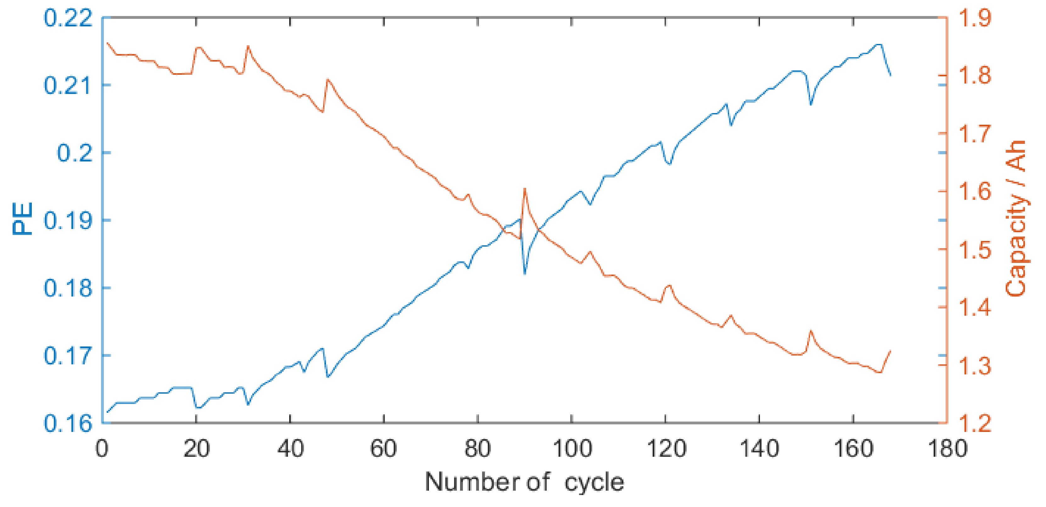
4.1. Verification of HI Extraction

PE features are extracted from discharge voltage sequence. In our study, we describe the PE features of battery No. 5 and 18 in Figure 5 and Figure 6, respectively. Observing these figures, the PE degrades with the cycle increasing during degradation process. As can be seen in Figure 5 and Figure 6, it has a good symmetry between the PE feature and the maximum releasable capacity. The PE feature as a novel HI can be an indicator for lithium-ion battery degradation process.

Figure 5. PE feature of battery No. 5.

Figure 6. PE feature of battery No. 18.

In order to further study whether PE feature can express the change of the battery capacity efficiently, the similarity between the PE feature and capacity are analyzed by Pearson and Spearman correlation. The correlation analyses of batteries No. 5, 6, 7, and 18 are presented in Table 1. Experiment results prove that it has a highly approximately negative linear relationship between the change of PE feature and capacity.

Table 1. Effectiveness analyses of HI based on PE.

Battery Number	No. 5	No. 6	No. 7	No. 18
Pearson correlation	−0.9977	−0.9931	−0.9979	−0.9909
Spearman correlation	−0.9994	−0.9999	-0.9995	−0.9919

Due to the loss of some early discharge voltage data of battery No. 6 and 7 at the self-recharge stage, some PE values in the degradation process are 0. In order to make the correlation analysis meaningful, the correlation analysis should be carried out after removing the data with the PE value of 0 and the corresponding capacity.

The proposed HI based on PE feature is effective and can express the capacity degradation process of lithium-ion battery well.

Table 2 has shown the advantage of the proposed HI based on PE compared with MVF [14] and DVD_ETI [12]. The results show that the similarity between PE and battery capacity is higher than that of MVF and DVD_ETI. Therefore, the proposed HI based on PE is more efficient in expression of battery degradation compared with MVF and DVD_ETI.

Table 2. Similarity analyses comparison by battery No. 5.

HI	PE	MVF	DVD_ETI
Pearson correlation	−0.9977	−0.9897	−0.9920
Spearman correlation	−0.9994	−0.9868	−0.9890

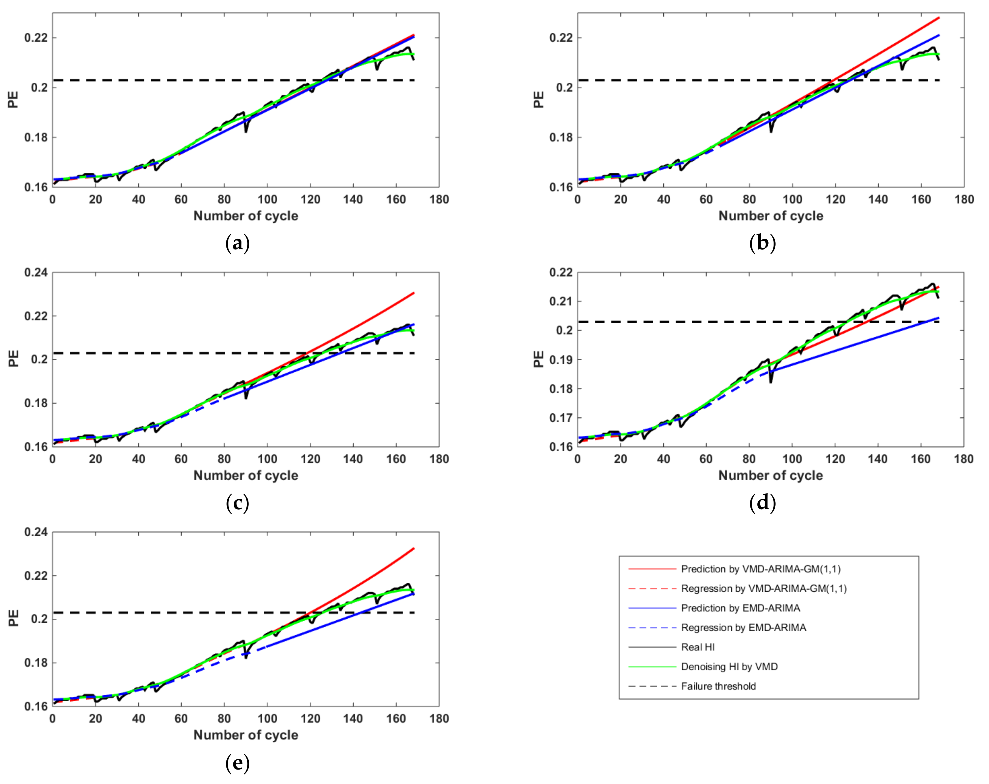
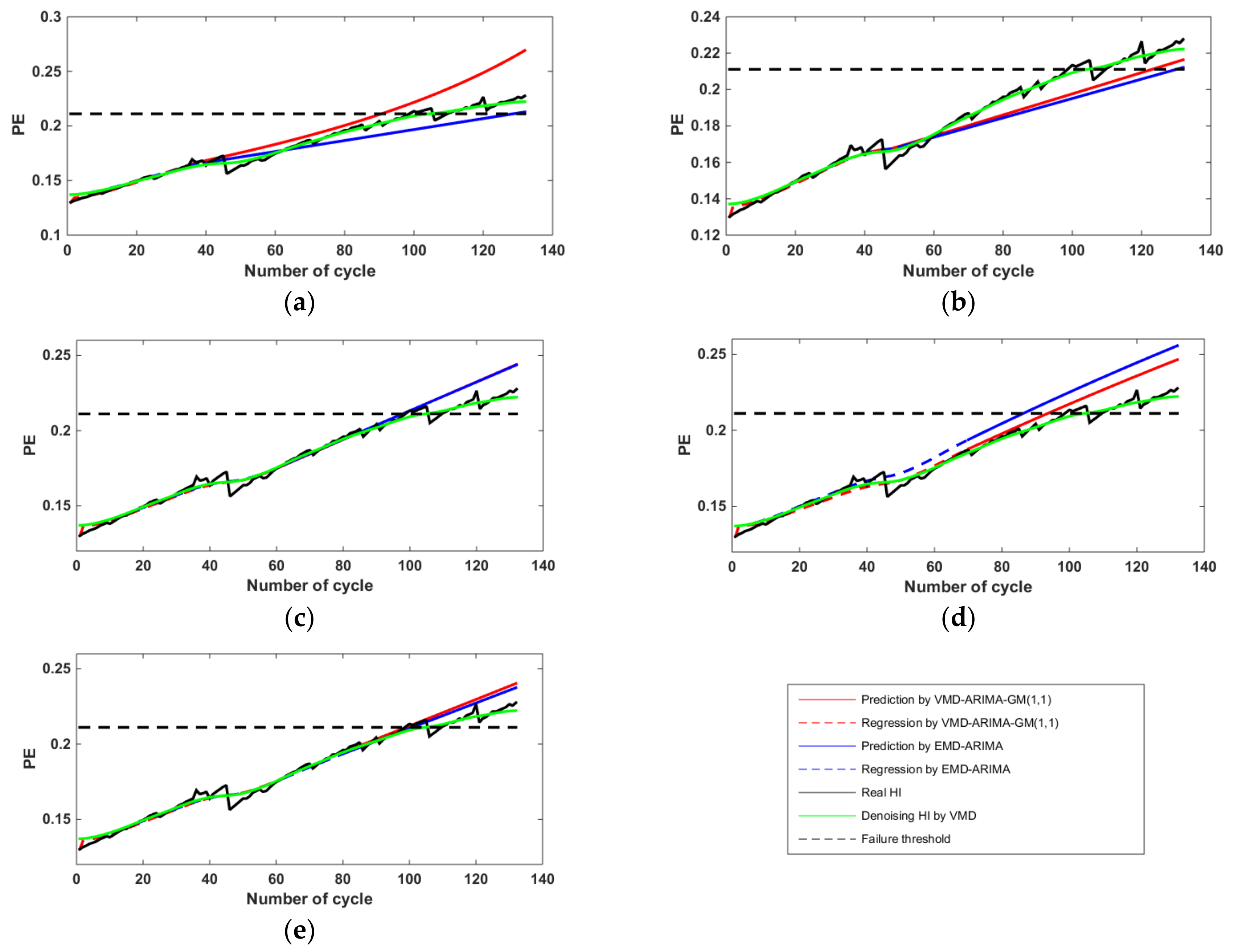
4.2. RUL Prediction Results and Analysis

4.2.1. Evaluation Criteria

After verifying the effectiveness of PE, we perform RUL prediction based on PE at different starting point for each battery. Due to the loss of some early discharge voltage data of battery No. 6 and 7 at the self-recharge stage, we use battery No. 5 and 18 as examples to make RUL prediction.

The absolute error (AE) and root mean squared error (RMSE) are defined as the evaluation criteria to estimate accuracy of the proposed approach,

• AE

  $$AE=\left|R-\widehat{R}\right|$$

  (20)
• RMSE

  $$RMSE=\sqrt{\frac{{{\displaystyle \sum }}_{i=1}^N{\left[x\left(i+n_s\right)-\widehat{x}\left(i+n_s\right)\right]}^2}{N}}$$

  (21)

  where $R$ is the actual RUL and $\widehat{R}$ is the predicted RUL. $x\left(i+n_s\right)$ is the actual HI and $\widehat{x}\left(i+n_s\right)$ is the predicted HI, respectively. N is the sampling size. $n_s$ is the prediction starting cycle.

To predict the battery RUL, we should confirm the PE failure threshold. As mentioned above, the discharge experiments were stopped when the battery capacity dropped by 30%. Due to the highly linear relationship between capacity and PE, we estimate the PE failure threshold is 0.2. Then the RUL can be obtained by counting the length between the starting point and failure threshold of PE.

4.2.2. Prediction Results and Analysis

We use VMD–ARIMA–GM(1,1) and EMD–ARIMA approaches to make RUL prediction based on PE at five different starting points for No. 5 and 18 batteries, respectively. The prediction results are shown in Figure 7 and Figure 8. Moreover, according to Equations (20) and (21), we conclude the performance of the proposed approach presented in Table 3.

Figure 7. RUL prediction for battery No. 5 at (a) 60 cycles; (b) 70 cycles; (c) 80 cycles; (d) 90 cycles; (e) 100 cycles.

Figure 8. RUL prediction for battery No. 18 at (a) 40 cycles; (b) 50 cycles; (c) 60 cycles; (d) 70 cycles; (e) 80 cycles.

Table 3. RUL prediction performance base on PE compared with Capacity.

Approach	HI	Battery No.	Starting Point	Actual RUL	Predicted RUL	AE	RMSE	TIME(s)
VMD–ARIMA–GM(1,1)	PE	#05	60	65	67	2	0.0026	5.7240
			70	55	49	6	0.0054	3.1329
			80	45	38	7	0.0067	3.0489
			90	35	45	10	0.0028	3.1980
			100	25	20	5	0.0079	3.9542
		#18	40	59	51	8	0.0182	4.6548
			50	49	73	24	0.0092	5.0305
			60	39	38	1	0.0087	6.0966
			70	29	24	5	0.0120	5.2689
			80	19	19	0	0.0083	4.2462
	Capacity	#05	60	65	59	6	0.0599	3.6518
			70	55	50	5	0.0552	5.5227
			80	45	44	4	0.0326	3.5595
			90	35	54	19	0.0509	4.9536
			100	25	27	2	0.0245	2.9617
		#18	40	59	88	29	0.0559	4.3129
			50	49	63	14	0.0435	5.5490
			60	39	31	8	0.1065	3.5446
			70	29	22	7	0.0917	4.1230
			80	19	14	5	0.0764	3.8354
EMD–ARIMA	PE	#05	60	65	68	3	0.0025	5.6949
			70	55	57	2	0.0027	3.0554
			80	45	54	9	0.0031	3.1098
			90	35	72	37	0.0089	3.2036
			100	25	43	18	0.0060	3.8054
		#18	40	59	89	30	0.0100	4.7045
			50	49	80	31	0.0115	5.0143
			60	39	38	1	0.0086	6.1818
			70	29	16	13	0.0192	5.2857
			80	19	21	2	0.0067	4.2334
	Capacity	#05	60	65	59	6	0.0593	3.7034
			70	55	54	1	0.0452	5.5080
			80	45	53	8	0.0356	3.5589
			90	35	72	37	0.0894	4.8837
			100	25	39	14	0.0470	3.0115
		#18	40	59	100	41	0.0734	4.3695
			50	49	73	24	0.0604	5.0888
			60	39	26	13	0.1392	3.5195
			70	29	25	4	0.0775	3.9590
			80	19	20	1	0.0551	3.9384

As shown in Figure 7 and Figure 8, the VMD–ARIMA–GM(1,1) and EMD–ARIMA approaches can both predict the battery RUL well. The green solid line represents the denoising HI sequence; the blue dashed line represents the regression curve of ARIMA model by the denoising HI training data; the blue solid line represents the ARIMA model prediction; the red dashed line represents the regression curve of the proposed model in this paper; the red solid line represents the proposed combining model prediction. Compared with the blue dashed line, the gap between the red dashed line and the green solid line is smaller, because the introduction of the GM(1,1) model compensates the residual value between the original sequence and the regression sequence of the ARIMA model.

As shown in Figure 7b and Figure 8b,d, the obvious regeneration phenomenon of battery capacity may lead to a large deviation of ARIMA regression sequence compared with the real one. The VMD–ARIMA–GM(1,1) proposed in this paper is a combination prediction approach, which can effectively reduce the prediction interference caused by the battery capacity regeneration.

Table 3 shows the performance of the proposed approach with different HIs and starting points for battery No. 5 and 18. The AEs with VMD–ARIMA–GM(1,1) range from 7.7 to 29 cycles, while the range of EMD–ARIMA is 14.8–41 cycles. The AEs of RUL with VMD–ARIMA–GM(1,1) are smaller than that with EMD–ARIMA. Therefore, we can conclude that VMD–ARIMA–GM(1,1) effectively improves the accuracy of RUL prediction.

All of the predicted HI made by VMD–ARIMA–GM(1,1) are very close to real HI sequence, which have been shown in Figure 7 and Figure 8. The RMSE value range from 0.0026 to 0.1065, while the range of EMD–ARIMA is 0.0025–0.1392. Therefore, we can conclude that our proposed approach outperforms the EMD–ARIMA approach in the long-term prediction of battery RUL.

In order to verify the computational efficiency of the proposed approach, the execution time of the proposed approach in Matlab has been calculated. Different training sequence leads to different time of building ARIMA model, so the execution time statistics can only be a range. Experiment results shows the execution time of VMD–ARIMA–GM(1,1) is 2.9617–6.0966 s while the range of EMD–ARIMA is 3.0554–6.1818 s. Compared with EMD–ARIMA, the proposed approach has a slight advantage in execution time.

According to the above analysis, we can conclude that the proposed RUL prediction approach based on PE and VMD–ARIMA–GM(1,1) undoubtedly as outstanding performance with effectiveness, high accuracy and long-term prediction ability.

5. Conclusions

In this paper, we propose a novel approach for lithium-ion battery on-line RUL prediction based on PE. The PE sequence is obtained by the discharge voltage series during battery degradation process. Based on the PE sequence, we proposed a hybrid model called VMD–ARIMA–GM(1,1) to estimate the battery RUL. The main findings in this paper are highlighted as follows:

• By Pearson and Spearman correlation analyses, we can find the correlation absolute value between PE and capacity is close to 1, indicating that PE has a high linear relationship with capacity. PE features can express the battery degradation process well.
• The Pearson correlation absolute value of PE, MVF, and DVD_ETI is 0.9977, 0.9897, and 0.9920, respectively. The Spearman correlation absolute value of PE, MVF and DVD_ETI is 0.9994, 0.9868, and 0.9890, respectively. Both results show that PE has better presentation ability than MVF and DVD_ETI.
• The AEs with VMD–ARIMA–GM(1,1) range from 7.7 to 29 cycles, while the range of EMD–ARIMA is 14.8–41cycles. The RMSE values range from 0.0026 to 0.1065, while the range of EMD–ARIMA is 0.0025–0.1392. The error analysis illustrates VMD–ARIMA–GM(1,1) usually has an advantage over EMD–ARIMA in accuracy.
• Different training sequence leads to different time of building ARIMA model, so the execution time statistics can only be a range. The execution time of VMD–ARIMA–GM(1,1) is 2.9617–6.0966 s, while the range of EMD–ARIMA is 3.0554–6.1818 s. Compared with EMD–ARIMA, the proposed approach has a slight advantage in execution time.

Algorithm fusion is a good trend for battery RUL estimation. Due to the GM(1,1) model being processed by using the approximate exponential law, it may lead to the excessive residual compensation for RUL prediction as shown in Figure 7e and Figure 8a. To overcome this problem, in our future research, we should further study the data-driven approach for battery long-term RUL prediction to replace the GM(1,1) model. Dynamic and probability estimation of PE will also be studied.

References

1. Genc, R.; Alas, M.O.; Harputlu, E.; Repp, S.; Kremer, N.; Castellano, M.; Colak, S.G.; Ocakoglu, K.; Erdem, E. High-capacitance hybrid supercapacitor based on multi-colored fluorescent carbon-dots. Sci. Rep. 2017, 7, 11222. [Google Scholar] [CrossRef] [PubMed]
2. Zou, C.; Manzie, C.; Nešić, D.; Kallapur, A.G. Multi-time-scale observer design for state-of-charge and state-of-health of a lithium-ion battery. J. Power Sources 2016, 335, 121–130. [Google Scholar] [CrossRef]
3. Prasad, G.K.; Rahn, C.D. Model based identification of aging parameters in lithium ion batteries. J. Power Sources 2013, 232, 79–85. [Google Scholar] [CrossRef]
4. Orchard, M.E.; Hevia-Koch, P.; Zhang, B.; Tang, L. Risk measures for particle-filtering-based state-of-charge prognosis in lithium-ion batteries. IEEE Trans. Ind. Electron. 2013, 60, 5260–5269. [Google Scholar] [CrossRef]
5. Hu, C.; Youn, B.D.; Wang, P. Ensemble of data-driven prognostic algorithms for robust prediction of remaining useful life. Reliabil. Eng. Syst. Saf. 2012, 103, 120–135. [Google Scholar] [CrossRef]
6. Patil, M.A.; Tagade, P.; Hariharan, K.S.; Kolake, S.M.; Song, T.; Yeo, T.; Doo, S. A novel multistage support vector machine based approach for li-ion battery remaining useful life estimation. Appl. Energy 2015, 159, 285–297. [Google Scholar] [CrossRef]
7. Wu, J.; Zhang, C.; Chen, Z. An online method for lithium-ion battery remaining useful life estimation using importance sampling and neural networks. Appl. Energy 2016, 173, 134–140. [Google Scholar] [CrossRef]
8. Zhang, C.; He, Y.; Yuan, L.; Xiang, S.; Wang, J. Prognostics of lithium-ion batteries based on wavelet denoising and de-rvm. Comput. Intell. Neurosci. 2015, 2015, 14. [Google Scholar] [CrossRef] [PubMed]
9. Zhang, C.; He, Y.; Yuan, L.; Xiang, S. Capacity prognostics of lithium-ion batteries using emd denoising and multiple kernel rvm. IEEE Access 2017, 5, 12061–12070. [Google Scholar] [CrossRef]
10. Zhou, Y.; Huang, M. Lithium-ion batteries remaining useful life prediction based on a mixture of empirical mode decomposition and arima model. Microelectron. Reliabil. 2016, 65, 265–273. [Google Scholar] [CrossRef]
11. Liu, D.; Wang, H.; Peng, Y.; Xie, W.; Liao, H. Satellite lithium-ion battery remaining cycle life prediction with novel indirect health indicator extraction. Energies 2013, 6, 3654–3668. [Google Scholar] [CrossRef]
12. Liu, D.; Zhou, J.; Liao, H.; Peng, Y.; Peng, X. A health indicator extraction and optimization framework for lithium-ion battery degradation modeling and prognostics. IEEE Trans. Syst. Man Cybern. Syst. 2015, 45, 915–928. [Google Scholar]
13. Zhang, Y.; Guo, B. Online capacity estimation of lithium-ion batteries based on novel feature extraction and adaptive multi-kernel relevance vector machine. Energies 2015, 8, 12439–12457. [Google Scholar] [CrossRef]
14. Zhou, Y.; Huang, M.; Chen, Y.; Tao, Y. A novel health indicator for on-line lithium-ion batteries remaining useful life prediction. J. Power Sources 2016, 321, 1–10. [Google Scholar] [CrossRef]
15. Widodo, A.; Shim, M.C.; Caesarendra, W.; Yang, B.S. Intelligent prognostics for battery health monitoring based on sample entropy. Expert Syst. Appl. Int. J. 2011, 38, 11763–11769. [Google Scholar] [CrossRef]
16. Tang, G.; Wang, X.; He, Y.; Liu, S. Rolling bearing fault diagnosis based on variational mode decomposition and permutation entropy. In Proceedings of the IEEE International Conference on Ubiquitous Robots and Ambient Intelligence, Xi’an, China, 19–22 August 2016; pp. 626–631. [Google Scholar]
17. Li, Y.; Li, Y.; Chen, X.; Yu, J. Denoising and feature extraction algorithms using npe combined with vmd and their applications in ship-radiated noise. Symmetry 2017, 9, 256. [Google Scholar] [CrossRef]
18. Bandt, C.; Pompe, B. Permutation entropy: A natural complexity measure for time series. Phys. Rev. Lett. 2002, 88, 174102. [Google Scholar] [CrossRef] [PubMed]
19. Dragomiretskiy, K.; Zosso, D. Variational mode decomposition. IEEE Trans. Signal Process. 2014, 62, 531–544. [Google Scholar] [CrossRef]
20. Box, G.E.P.; Jenkins, G.M. Time series analysis: Forecasting and control. J. Time 2010, 31, 303. [Google Scholar]
21. Calheiros, R.N.; Masoumi, E.; Ranjan, R.; Buyya, R. Workload prediction using arima model and its impact on cloud applications’ qos. IEEE Trans. Cloud Comput. 2015, 3, 449–458. [Google Scholar] [CrossRef]
22. Chen, Y.; Wei, Y. Applications of grey relative relational grade to optimization of grey model gm(1,1). J. Grey Syst. 2007, 19, 321–332. [Google Scholar]
23. Saha, B.; Kai, G.; Poll, S.; Christophersen, J. Prognostics methods for battery health monitoring using a bayesian framework. IEEE Trans. Instrum. Measur. 2009, 58, 291–296. [Google Scholar] [CrossRef]