Article

Direct Flux Control for Stand-Alone Operation Brushless Doubly Fed Induction Generators Using a Resonant-Based Sliding-Mode Control Approach

State Key Laboratory of Advanced Electromagnetic Engineering and Technology, Huazhong University of Science and Technology, Wuhan 430074, China
*
Author to whom correspondence should be addressed.
Energies 2018, 11(4), 814; https://doi.org/10.3390/en11040814
Submission received: 6 February 2018 / Revised: 26 March 2018 / Accepted: 29 March 2018 / Published: 2 April 2018

Abstract

:
In this paper, a novel voltage control strategy for stand-alone operation brushless doubly fed induction generators for variable speed constant frequency wind energy conversion systems was presented and discussed. Based on the model of the power generation system, the proposed direct flux control strategy employs a nonlinear reduced-order generalized integrator-based resonant sliding-mode control approach to directly calculate and regulate the output value of converter which the control winding stator requires so as to eliminate its instantaneous errors, without involving any synchronous rotating coordinate transformations. The stability, robustness and convergence capability of the proposed control strategy were described and analyzed. Owing to the fact no additional current control inner loops are involved, the system configuration is therefore simplified and the dynamic performance enhanced. A constant converter switching frequency was achieved by using space vector pulse width modulation, which reduces the harmonics of the generator terminal voltage. In addition, the feasibility and validity of the proposed scheme is verified by experiments, and excellent steady and transient performance is achieved.

1. Introduction

Among variable-speed constant-frequency (VSCF) wind energy conversion systems (WECS), a brushless doubly-fed induction generator (BDFIG) is a reliable option that inherits the doubly-fed induction generator (DFIG)’s benefits of low cost structure due to the facts that no permanent magnets materials are utilized and only a fractionally rated converter is needed. Simultaneously, the absence of electric slip rings eliminates one of the main failure modes of the DFIG [1,2]. The BDFIG also has a significantly enhanced low-voltage ride-through performance in contrast with a DFIG [3]. Furthermore, it is a medium velocity machine, which increases the efficiency due to the avoidance of a high-speed gear stage.
The control of BDFIG systems has recently received much more attention than ever. In particular, a classical vector control (VC) oriented power winding (PW) stator flux is presented in [4,5,6,7,8], where the instantaneous PW stator active and reactive powers are controlled by regulating the decoupled control winding (CW) currents, and proportional-integral (PI) controllers are employed. Moreover, VC-based unbalanced operation is investigated [6,7], and the typical improved algorithm includes employing PI regulators implemented in the positive and negative sequence counter-rotating synchronous reference frame, respectively [6], or PI plus resonant (PIR) regulators to implement the precise control of currents in a positive sequence synchronous reference frame [7]. Besides, VC-based sensor-less control is developed as well [8]. The main drawback for VC is that the performance highly relies on the harmony of the controller parameters and accurate generator parameters. Besides, in view of the discrete operation of source converters, direct control (DC) was proposed in [9,10,11,12,13]. Such a scheme directly controls the generator torque or power, reduces the complexity of the VC and minimizes the effect of generator parameters. Initially, the traditional lookup table (LUT) DC, selects the proper voltage vectors directly from a predefined optimal switching signals LUT based upon the information of the machine [9,10], and can further implemented in unbalanced situations [11]. Moreover, in [12] the synthetic vector direct control solved the out of control issues. Nevertheless, the main drawback lies in the fact the converter switching frequency varies with the hysteresis bandwidth and operation, as a result, a PW stator side filter is needed to prevent a broad-band harmonics spectrum from injecting into the grid. Besides, a high sampling frequency is required to ensure admissible performances. To solve this issue, a predictive DC strategy was presented in [13], where the duration times of each voltage vector were optimized with the cost function target of reduce ripple in the torque and flux. Although possibly constant switching frequency is achieved, complicated online calculations are needed. Model predictive control directly calculates the required voltage vectors within each sampling period [14], however, it is quite sensitive to machine parameter variations, moreover, it necessitates the rotating coordinate transformations. Besides, an indirect stator-quantities control [15] implemented in stationary reference frames, and inner loops regulator incorporating pulse width modulation (PWM) was developed. Apparently, like VC, a simple linear approximation of the error can cause the system performance to degrade due to the nonlinear nature of converters.
The study primarily addressed grid-connected operation mode. On the other hand, the development of WECS and the distributed generation concept especially resulted in isolated grids, Therefore, the stand-alone operation application is imperative. Meanwhile, relatively less work has been focused on the stand-alone operation. The VC scheme is designed and verified in [16,17]. Furthermore, a PIR regulator is employed to eliminate harmonics [18]. Nevertheless, VC schemes have the weak robustness to parameter variations, etc. The predictive DC scheme [14] required complicated calculations, while a direct voltage control scheme [19] neglected the impact of load current on the terminal voltage. Moreover, the above methods were implemented in the synchronously reference as well.
The sliding-mode (SM) control (SMC) strategy is an effective scheme for nonlinear systems with uncertainties. It features simple implementation, disturbance rejection, strong robustness, and sensitive responses. An SMC approach for DFIGs driven by turbines has been proposed in [20,21,22,23,24,25,26,27]. In particular, a first-order SMC leads to a variable switching frequency [21] and broadband harmonics. This problem is solved through application of a boundary layer [22]. Nevertheless, the ultimate tracking accuracy was partially lost. Furthermore, SM surfaces are set as the integral forms to minimize errors and maintain an enhanced response [23]. Besides, for the sake of suppressing chattering, the second-order SMC was proposed in [24], and to deal with either unbalanced or distorted grid voltages as well [25], however tuning the control parameters is a challenge. The fractional order SMC offers more flexibility, and hence optimizes the dynamic response [26,27], but it is not supported by sufficient experimental validation yet. Apparently, like the VC scheme, all of the process still requires rotating coordinate transformation. So far there is less literature associated with SMC for BDFIG.
In order to tackle the disadvantages highlighted earlier, this paper presents a novel direct flux control (DFC) scheme for stand-alone operation BDFIG using a resonant(R)-based SMC approach. It simply regulates the instantaneous PW stator flux without extra CW current control or involving rotating coordinate transformations. The required CW stator voltage can be directly procured in the PW stator stationary reference frame and a nonlinear reduced order generalized integrator (ROGI)-based sliding surface is introduced. The constant switching frequency is achieved by a space vector modulation (SVM) technique. As a result, enhanced dynamic performance alike to the DC scheme is obtained and steady state harmonic spectra are maintained at the same level as with the VC strategy. The rest part of the paper is organized as follows: in Section 2, the operation of BDFIG is briefly summarized, and the model and dynamic behavior is given. In Section 3, the ROGI-based R SM DFC approach is devised and analyzed entirely. Section 4 demonstrates the performance of the scheme by experiments. Finally, the conclusions are presented in Section 5.

2. BDFIG Stand-Alone Operation and Model

2.1. Operation and Configuration

The stator of the BDFIG is furnished with two separate stator windings, known as the PW and CW, which share one stator lamination and differ in pole pair number distribution to avoid direct coupling between the windings. The special rotor couples both stator windings [2]. In general, the PW stator connected to the point of common coupling (PCC) directly, whereas the CW stator is fed by a back-to-back voltage source converter (VSC), handling only a fraction of the rated power with limited velocity ranges. This topology shown in Figure 1 has the merit of decreasing the rating of the VSC. The CW stator side converter (CSC) is designed to control the PW stator terminal voltage and frequency constant with variable-speed turbine. The load side converter (LSC) keeps the direct-current (DC)-link voltage constant, meets the grid side harmonic acceptance indicator and guarantees the converter operation with an expected power factor. Quite unlike the grid-connected mode application, a stand-alone power generation system itself has to generate a voltage and frequency in the PW stator terminal irrespective of varying rotational velocity due to turbine speeds and varying loads. Hence, for the sake of guarantee entire desired performance, the PW stator terminal voltage’s amplitude and frequency stability are greatly compulsive.
The BDFIG is normally operated in the synchronous mode, in which the shaft velocity is determined by the excitation frequencies of the two stator windings, independent of the torque exerted on the generator, the so-called synchronous rotor angular velocity can be expressed as:
ω r = ω p + ω c p p + p c
where ωp and ωc are the excitation angular frequencies provide to PW (pp pole pairs) stator and the CW (pc pole pairs) stator respectively. Stator and rotor quantities are shown for the synchronous mode in Figure 2.

2.2. Model and Dynamic Behavior of a BDFIG

The equivalent circuit of a BDFIG represented in the unified reference frame with arbitrarily angular velocity rotating is shown in Figure 3, where the generic dynamic vector model [28] in pp-type pole pairs distribution can be expressed. The voltage vectors is given as:
U p p = R p I p p + d Ψ p p / d t + j ω Ψ p p
U c p = R c I c p + d Ψ c p / d t + j [ ω ( p p + p c ) ω r ] Ψ c p
U r p = R r I r p + d Ψ r p / d t + j ( ω p p ω r ) Ψ r p
The flux linkage vectors is given as:
Ψ p p = L s p I p p + L m p I r p
Ψ c p = L s c I c p + L m c I r p
Ψ r p = L r I r p + L m c I c p + L m p I p p
The electromagnetic torque equation is expressed:
T e = 3 2 p p I m [ Ψ p p I p p ] + 3 2 p c I m [ Ψ c p I c p ]
Considering the rotor voltage Equation (4), Ur = 0, then rotor flux Ψ r p can be expressed as:
Ψ r p = R r I r p [ d / d t + j ( ω p p ω r ) ]
Noting that in a well-designed BDFIG, the Rr has small values and is negligible, meanwhile, the value of d / d t + j ( ω p p ω r ) is larger both in steady state and transient state. Evaluating the different factor values of Equation (9), it can be concluded that Ψ r p is so smaller that can be assumed Ψ r p ≈ 0, then, according to rotor flux Equation (7) the rotor current can be derived as:
I r p = L m c L r I c p L m p L r I p p
Substituting Equation (10) Ir to flux Equations (5) and (6), PW and CW stator flux linkage vectors can be can be simplified as follows:
Ψ p p = A p I p p + A m I c p
Ψ c p = A c I c p + A m I p p
where A p = L s p L m p 2 / L r , A c = L s c L m c 2 / L r , and A m = L m c L m p / L r . In the flux Equations (11) and (12), the two stator electromagnetic coupling relationship is represented directly.
Based on PW stator flux Equation (11), the CW stator current can be expressed as:
I c p = Ψ p p A p I p p A m
Substituting Equation (13) to CW stator flux Equation (12) and systematizing it, then the instantaneous CW stator flux linkage can be expressed as:
Ψ c p = A c A m Ψ p p A c A p A m 2 A m I p p
Differentiating Equation (14) results in instantaneous variations of CW stator flux as:
d Ψ c p d t = A c A m d Ψ p p d t A c A p A m 2 A m d I p p d t
Substituting Equations (14) and (15) to CW stator voltages Equation (6), and systematizing it, then, the instantaneous variations of PW stator flux can be derived as:
d Ψ p p d t = A m A c U c p { A m A c R c + j A m [ ω ( p p + p c ) ω r ] } I c p j A m 2 A c [ ω ( p p + p c ) ω r ] I p p + A c A p A m 2 A c d I p p d t
It is worthy noting that, the model and dynamic behavior can be represented in the PW synchronous rotating reference frame by setting ω = ωp, or in PW stationary reference frame by setting ω = 0 in Equations (2)–(16).

3. Proposed DFC Using R-SMC Approach

3.1. Reference Flux Quantity

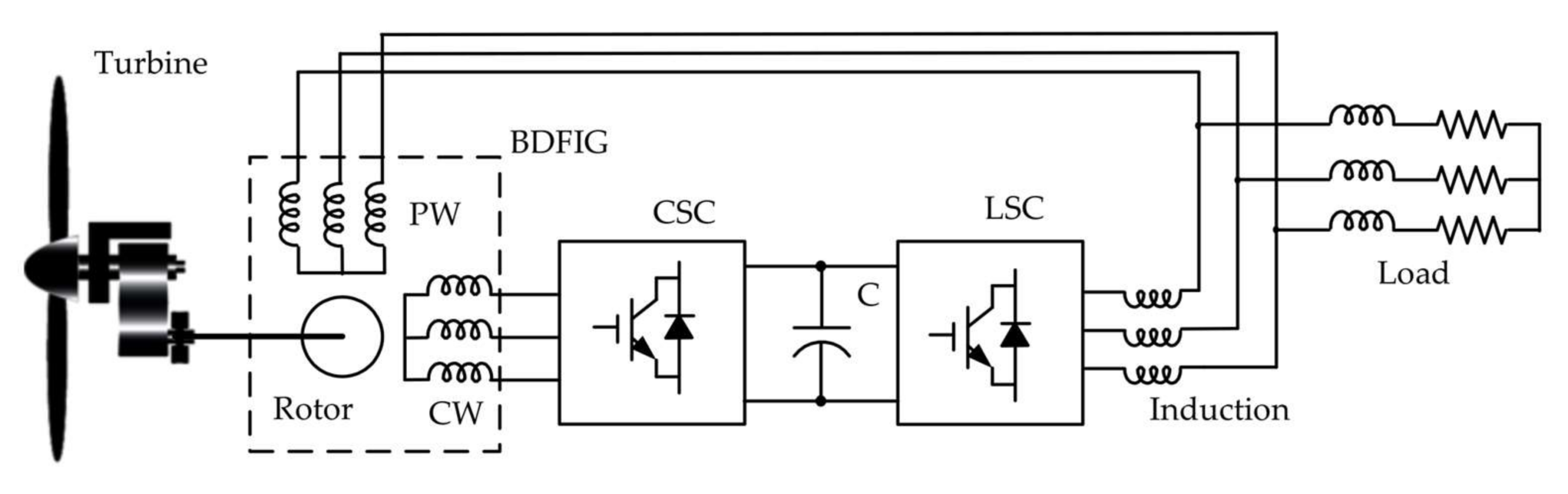
The stand-alone operation BDFIG must supply constant amplitude and frequency of voltage at the PW stator terminals irrespective of the varying shaft rotational velocity due to wind turbine speeds and varying loads. The PW stator voltage is indirectly determined through PW stator flux which is regulated by CW stator excitation current, thus the reference quantity can be set as PW stator flux. PW stator voltage phase angle can be derived directly from a free-running integral of the PW stator frequency reference, and according to PW stator voltage Equation (2), the commanded PW stator flux value is calculated from integration of the PW stator back electromotive force (EMF) references:
Ψ p α β p = ( U p α β p R p I p α β p ) d t
As the flux estimation proposed in Equation (17) will produce direct-current (DC) drift at low frequency in this implementation, the DC drift is extracted and eliminated with a low-pass filter instead of a pure integrator. In addition, generally speaking, the integral model is irrelevant to additional generator parameters, except for the PW stator resistance whose impact on the system performance is inappreciable thanks to the smaller voltage drop relatively high grid frequency.

3.2. Sliding Surface

The control objectives for stand-alone operation BDFIG systems are to track or slide along the predefined PW stator flux trajectories. Thus the sliding switching surface is set as:
S = [ S 1 S 2 ] T
The derivation of resonant sliding surface is based on the stationary reference frame implementation of a synchronous integrator. In the PW synchronous rotating reference frame, both the current references and disturbance is characterized by a DC signals in steady state, for purpose of minimizing the steady state error while the enhanced transient response remains, the sliding switching surfaces can be set as the integral form generally [22,23]:
S d q = ( 1 + K / s ) E Ψ d q p
where, E p d q p = Ψ p d q p Ψ p d q p is the instantaneous error between the references and the actual values, K is positive control gain coefficient matrix. An integrator implemented in synchronous reference frame with input X d q and output Y d q is described by:
s Y d q = X d q
Nevertheless, integral sliding surfaces can only regulate the DC signals of the feedbacks to track the references in the synchronous reference frame but not alternating-current (AC) signals in stationary reference frame due to the lower amplitude responses at high frequency. Note that the relation between the variables in the synchronous rotating frame and the stationary frame is X d q = e j θ X α β , thus the integrator may be transformed to stationary reference frame by taking a frequency shift of −ω for the positive sequence, the stationary frame generalized integrator (SGI) is mostly performed from equivalent synchronous rotating frame integrator whose transfer function be given as:
G R O G I ( s ) = K s j ω
SGI, herein is also named ROGI relative to second-order generalized integrator (SOGI). It must be noted that with two ROGI a SOGI can be constructed:
G S O G I ( s ) = 2 s K s 2 + ω 2 = K s j ω + K s + j ω
The fewer states in the ROGI’s implementation against the SOGI’s and the close relation between both are the reasons why is named ROGI. Therefore, the ROGI requires less computational burden [
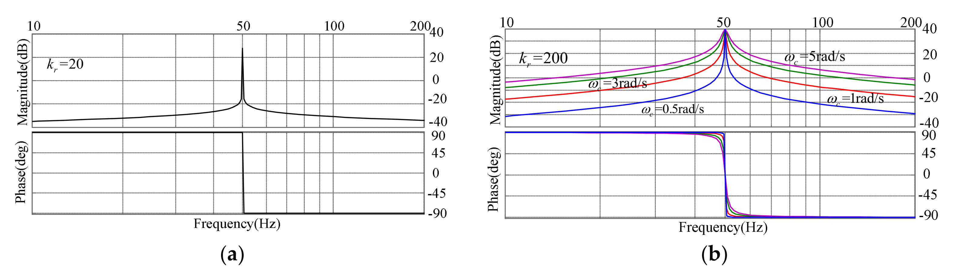
29]. In addition, both SOGI and ROGI are resonant controllers that eliminate the sinusoidal tracking error thanks to their infinite gain and zero phase shift to special order resonant frequency signals, but ROGI can provide discrimination between positive and negative sequence signals. The ROGI frequency response (magnitude and phase) be shown in Figure 4a. In fact, utilization of resonant controllers in AC tracking systems is a straightforward conclusion of internal model principle, explaining that provided to achieve zero steady-state error in a stable feedback system, the loop gain must contain a model, which can generate the required reference and disturbance signals, requiring integrative controller in DC systems and resonant controller in AC systems [29]. In the stationary frame, both the reference and disturbance behave like AC signals. Therefore, there should be a sinusoidal internal model in the controller so as to eliminate the tracking error in special orders. Besides, the magnitude and phase response changes precipitously at the adjacent of resonant frequency, therefore the steady accuracy and stability would be deteriorated as a result of frequency deviates. For the purpose of weaken the sensitivity toward slight frequency variations and increase the bandwidth around the resonant frequency, a component with cutoff frequency ωcf is inserted to well compromise in practice. As seen from the Bode diagram of improved quasi ROGI with different bandwidth coefficients in Figure 4b, the response is much smoother changing at the adjacent of resonant frequency.
Then, an improved ROGI resonant sliding surface which be tuned at fundamental frequency is defined as Equation (23) for PW stator stationary reference frame:
S α β = ( 1 + K ω c p s j ω p + ω c p ) E Ψ α β p
In general, the main advantages of this proposed ROGI are as follows: it provides infinite gain and zero phase shift to special order resonant frequency signals, which can eliminate the sinusoidal tracking error and offer discrimination between positive and negative sequences. As a consequence, implemented in stationary reference frame hence no extra synchronous rotating coordinate transformations and angular information involved, reducing the overall computational burden. The fewer states of the ROGI, which imply a minimum computational burden, make it ideal for low cost digital signal processor (DSP) implementation. A component with cutoff frequency is introduced, which reduces the sensitivity toward slight frequency variations and increases the bandwidth around the resonant frequency, thus ensuring the better robustness of steady state accuracy against frequency deviations.

3.3. SMC Law

As the name SMC indicates, the objective is to force the system state trajectory to the interaction of the switching surfaces. This section presents the design of an SMC scheme to generate the CW stator voltage reference.
The manifold S = 0 represent the precise tracking of PW stator flux. When the system states reach the sliding manifold and slide along the surface, then leads to:
S α β = d S α β / d t = 0
According to Equations (23) and (24), derivatives of S equal zero, thus we obtain:
d E Ψ α β p / d t = K E Ψ α β p
The equations mentioned before guarantee the PW stator flux errors converges to zero, and a positive control gain matrix K is selected for the expected system transients. The PW stator flux will converge asymptotically to the reference value with time constant matrix of 1/K. Then, the device objective is aimed at accomplishing sliding mode in the manifolds S = 0 with discontinuous CW stator voltage vectors:
d S α β d t = d E Ψ α β p d t + K E Ψ α β p = d Ψ p α β p d t + K ( Ψ p α β p Ψ p α β p )
Setting ω = 0 in Equation (16) for stationary reference frame and substituting it into Equation (26), then leads to:
d S α β / d t = F + B U c α β p
where:
B = A m / A c , U c α β p = [ u c α u c β ] T
and:
F = [ A m A c R c j A m ( p p + p c ) ω r ] I c α β p j A m 2 A c ( p p + p c ) ω r I p α β p A c A p A m 2 A c d I p α β p d t + K ( Ψ p α β p Ψ p α β p )
Splitting F into α-β components and arranging them in matrix form yields:
F = [ F 1 F 2 ] T
[ F 1 F 2 ] = [ A m A c R c A m ( p p + p c ) ω r A m ( p p + p c ) ω r A m A c R c ] [ i c α i c β ] + [ A m 2 A c ( p p + p c ) ω r A m 2 A c ( p p + p c ) ω r ] [ i p α i p β ] [ A c A p A m 2 A c A c A p A m 2 A c ] d d t [ i p α i p β ] + [ K α ( ψ p α ψ p α ) K β ( ψ p β ψ p α ) ]
A Lyapunov method is employed for deducing the control law that will drive the state orbit to the equilibrium manifold [22]. The quadratic Lyapunov function is chosen as:
W = S T S / 2 0
The time derivative of W on the state trajectories of Equation (28) is obtained by:
d W d t = 1 2 ( S T d S d t + S d S T d t ) = S T d S d t = S T ( F + B U c α β p )
The switch control law must be selected so as to ensure the time derivative of W is definitely negative with S ≠ 0. Therefore, the following control law is chosen:
U c α β p = B 1 { [ F 1 F 2 ] + [ K α 0 0 K β ] [ s g n ( S 1 ) s g n ( S 2 ) ] }
where sgn(S1) and sgn(S2) are respectively sign functions for α-β components flux error of PW stator. From Equation (30), the SM control law can be divided into two parts: the equivalent control part and the nonlinear switching control part. The equivalent control is used to control the nominal plant model, and the nonlinear switching control is added to ensure the satisfactory performance in spite of parametric uncertainty.

3.4. Proof of the Stability

For stability to the sliding surfaces, it is sufficient to have dW/dt < 0. By setting appropriate switch functions, the stability can be achieved provided the following condition is satisfied:
If S1sgn(S1) > 0 and S2sgn(S2) > 0 then:
d W d t = S T d S d t = S T [ K α 0 0 K β ] [ s g n ( S 1 ) s g n ( S 2 ) ]
The time derivative of Lyapunov function dW/dt is definitely negative, as a consequence, the control system becomes asymptotically stable.

3.5. Proof of the Robustness

In practice, the sliding surface S will be affected by the parameter variations, sample errors noises, etc. Therefore, Equation (27) should be rearranged as:
d S / d t = F + B U c α β p + H
where H = [ H 1 H 2 ] T represent system disturbances.
Thus, Equation (30) can be rewritten as:
d W d t = S T d S d t = S T { [ H 1 H 2 ] [ K α 0 0 K β ] [ s g n ( S 1 ) s g n ( S 2 ) ] }
Noting that provided K α > | H 1 | and K α > | H 1 | , i.e., the positive control gains meet the aforementioned condition, the time derivative of Lyapunov function dW/dt is still definitely negative. Thus, the SMC features strong robustness.

3.6. Remedy of Chattering Problem

The fast switching tracking of the instantaneous components may generate unexpected chattering, which may excite unmodeled high-frequency system transients and even result in unforeseen instability. To eliminate this behavior, the discontinuous control is smoothed out by introducing a boundary layer around the sliding surface [22]. As a result, a continuous saturated function around the sliding surface neighborhood is obtained as:
s g n ( S j ) = { 1 , if   S j > λ j S j / λ j , if   | S j | λ j 1 , if   S j < λ j
where λj > 0 is the width of the boundary layer and j = 1, 2. Then, the improve control law is obtained as Equation (35) with continuous saturated function instead of switch sign function in Equation (28), and the aforementioned condition of robustness and stability changes correspondingly as well:
U c α β p = B 1 { [ F 1 F 2 ] + [ K α 0 0 K β ] [ s a t ( S 1 ) s a t ( S 2 ) ] }

3.7. Analyses of Response Sensitivity

The SMC strategy, based on system dynamic characteristics, design sliding surface and the equivalent control, drives the system operation states to converge toward special manifolds in the state space from the hyperplane. According to the conditions for the existence of sliding mode and device discontinuous control, in case of reach the sliding surface, the control system will not be influenced by system parameters and external disturbances, slipping along the slide facing to the origin, and have the desired performance. From the deduction of SM control law Equation (35), the algorithm is not sensitive to machine rating, e.g., power, torque, velocity range. Although equivalent control is relevant to the generator parameters, the nonlinear switching control is added to ensure the desired performance despite parametric uncertainty.
Provided the initial value of the system state variable is Ψ 0 α β p = [ ψ 0 α ψ 0 β ] T , substituting SM control law to state Equation (27), then we have:
d S / d t = K s a t ( S )
The time of the system arrival SM switching surface can be deduced as:
T | Ψ 0 | + λ j ( l n λ j 1 ) K
It denotes the dynamic state performance, viz., response sensitivity of the propose strategy. According to Equation (37), obviously, the system not only converges in finite time, but also the increase of k can help reduce the time of system convergence to the SM switching surface, and enhance the response sensitivity, while on the other hand, within the boundary layer, the system no longer absolutely behaves as dictated by the sliding mode. Consequently, the characteristics of response sensitivity, tracking accuracy, etc. are partly compromised. In addition, it is worth noting that direct single control loop rather than extra control inner loop involved results in enhanced controlling bandwidth, and improved response sensitivity.

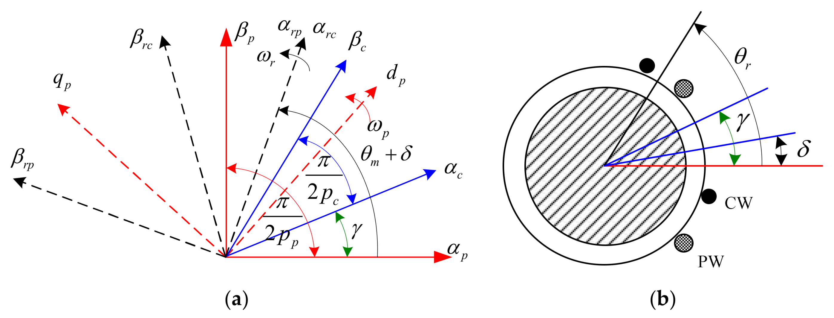
3.8. Stationary Reference Frame Coordinate Transformations

In this control scheme, the CW stator voltage and current magnitudes are expressed in a PW stator stationary reference frame. To express a magnitude Z from the CW stator (pc-type pole pairs) stationary reference frame transform into PW stator (pp-type pole pairs) stationary reference frame, the following relation can be used:
Z c α β c = Z c α β p e j ( p p + p c ) ( θ r + δ ) + p c γ
The spatial relationship of CW stator and PW stator stationary reference frames is shown in Figure 5a, noting that rotor position angular measurement is needed to transform a CW stator to a PW stator stationary reference frame, and initial rotor position angular is also needed to correct alignment [4]. The different reference axis and initial angular is shown in Figure 5b.

3.9. CW Stator-Side Output Voltage Limit

For a BDFIG, the maximum output voltage from the CSC is usually within the range of 30% of the PW stator voltage. Under steady-state operation, the required CW stator voltage is unlikely to exceed the output voltage limit of the CSC. However, during dynamic conditions, large and abrupt power variations of load can issue in large PW voltage errors. Consequently, the CW stator voltage calculated using Equations (30) and (35) may exceed the maximum output voltage capability of the CSC denoted as Ucmax. In practical operation, the limiter is also needed to eliminate stress on the mechanical and electrical elements [23]. Therefore, the CW stator voltage must be scaled proportionally to improve the transient response. This process can be represented as:
{ u c α = u c α u c α 2 + u c β 2 U c m a x u c β = u c β u c α 2 + u c β 2 U c m a x
CW stator voltage limit could result in PW stator voltage magnitude being temporarily sag, in this case, the LSC serve as a static volt-ampere reactive generator by injecting a compensate current at the PCC to support voltage.

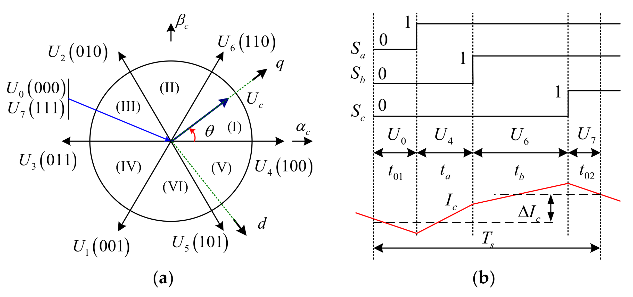
3.10. Voltage Vector Calculation Using SVM

The SVM is employed to generate the respective duration times of required switching voltage vectors. For a VSC feeding CW stator, which the three phase two-level configuration shown in Figure 6, the output voltages can be expressed by fundamental six active voltage vectors and two zero voltage vectors, indicated as U0U7 in Figure 7a, where the subscript of U originates from the binary number expressing the switching pattern in the phase sequence (a, b, c).
For the example shown in Figure 5a, where the average CW stator voltage vector Uc is located between U6 and U2, the voltage vectors required to reassemble Uc are U7, U6, U2, and U0, and their respective durations are calculated as Equation (40):
t a = 3 k v T s s i n ( π 3 θ ) , t b = 3 k v T s s i n ( θ ) , t 01 = t 01 = T s 2 [ 1 3 k v s i n ( π 3 + θ ) ]
where k v = | U c | / U d c , and 0 θ π / 3 .
CW stator voltage vectors and the impact of CW voltage vectors on the CW stator current is shown in Figure 7b.
In the case of over-modulation, the zero voltage vector durations t01 and t02 calculated using Equation (40) can become negative. Thus, the ta and tb must be scaled as:
t a = t a t a + t b T s , t b = t b t a + t b T s , t 01 = t 01 = 0
The SVM is differ from LUT hysteresis modulation which results in deterministic narrowband harmonic spectra with predominant harmonics around the fixed switching carrier frequency and multiples thereof.

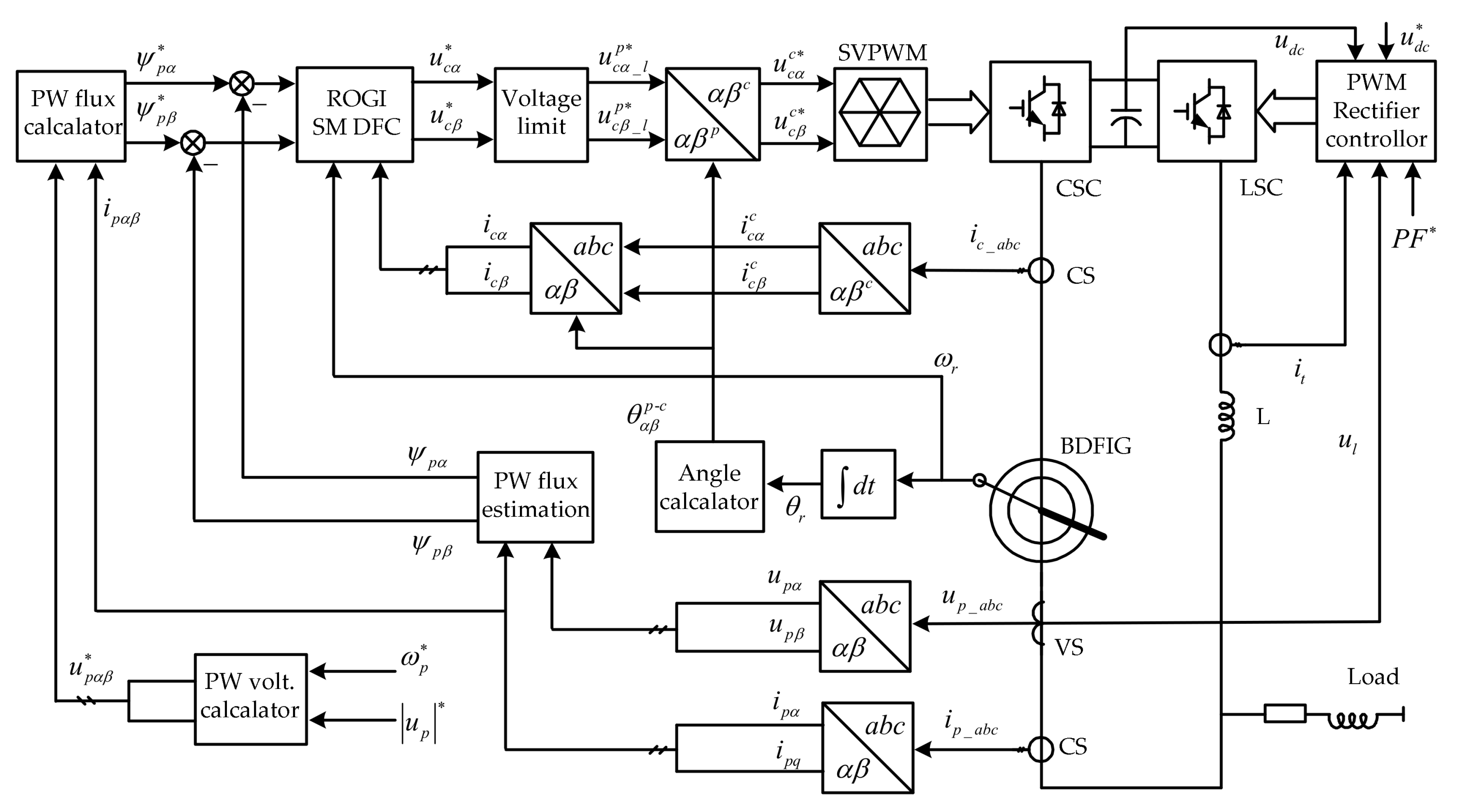
3.11. Control System Implementation

Based on the developed control strategies, the overall schematic diagram of proposed DFC strategy for a stand-alone operation BDFIG system employing the ROGI based R SMC approach is shown in Figure 8. As can be seen and was previously described, both PW stator voltage, current and CW stator currents is sampled and transformed to the PW stator stationary reference, respectively. The reference of the phase angle is derived directly from a free running integral of the PW stator frequency reference. The rotor position angle θr can be measured by the encoder. The PW stator flux value can be directly estimated according to integration of the PW stator back EMF which is irrelevant to additional generator parameters, except for the stator resistance. The instantaneous error of PW stator flux can be calculated by comparing the feedback quantity and reference quantity. The control law developed in Equation (35) based on the ROGI resonant sliding surface as Equation (23) is employed, and it simply regulates the instantaneous error of PW stator flux and directly generates the CW stator voltage reference for the CSC without any extra CW stator current control inter loops so as to enhance the transient performance. Afterward, it is transformed into a CW stator stationary reference. Moreover, the reference of the CW stator voltage is limited properly to improve the transient response. In addition, the SVM technique is employed to generate the switching patterns and their respective duration times, besides, achieve constant switching frequency which results in deterministic narrowband harmonic spectra with dominant harmonics around the carrier frequency and multiples thereof in CW stator voltage. Finally, it is worth noting that the proposed control scheme is implemented in the PW stator stationary reference frame hence no extra synchronous rotating coordinate transformations and angular information are involved.
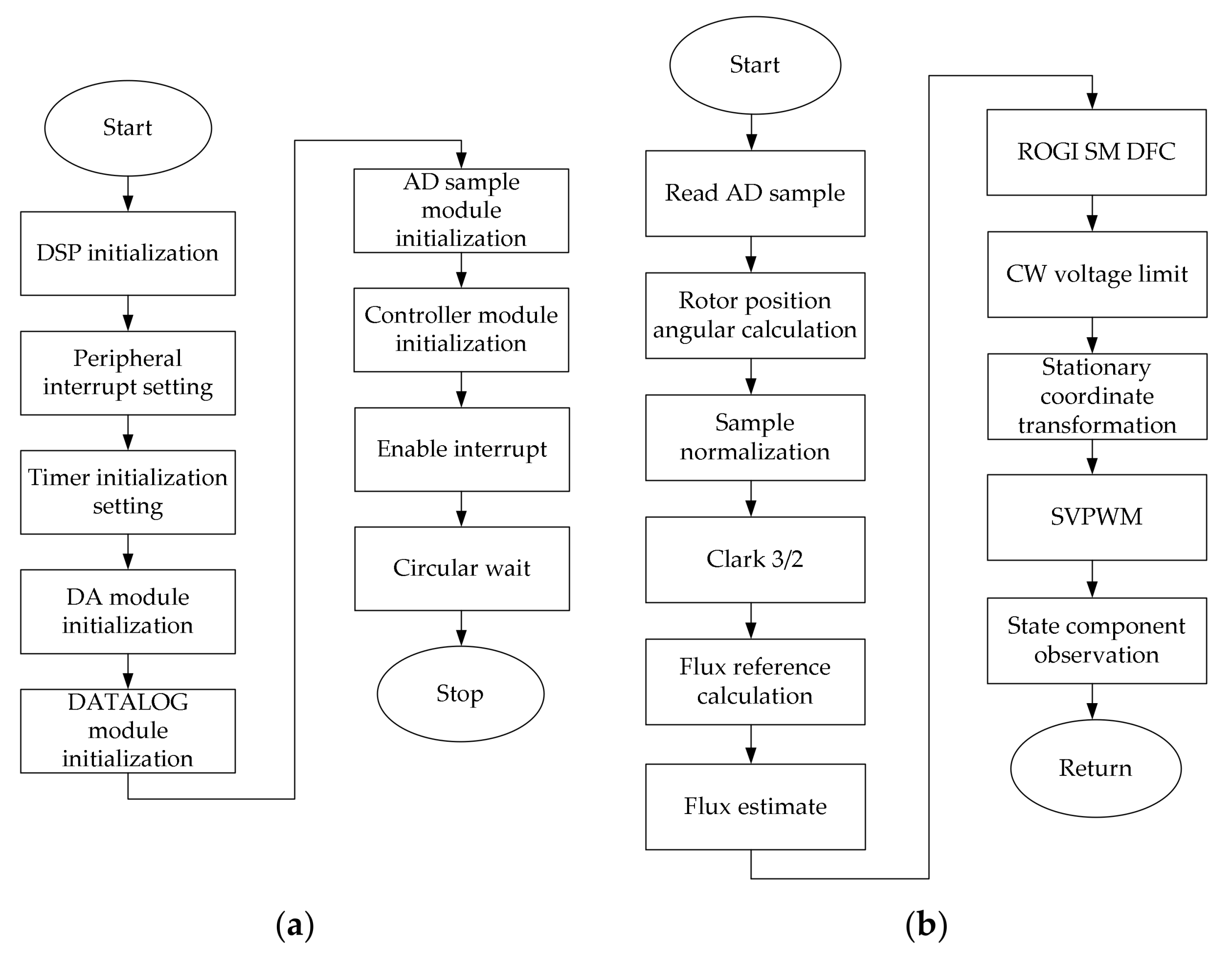
In order to effectively demonstrate the integration process of proposed control strategy, a flow chart is provided as shown in Figure 9.

3.12. Compared with Conventional Algorithms

Compared with the conventional VC strategy, the proposed novel algorithm is to be implemented in the PW stator stationary reference frame, quite unlike VC in the PW stator synchronous reference frame, thus, no synchronous rotating coordinate transformations and angular information are required. Furthermore, it directly regulate PW stator flux by calculating and adjusting the CW stator voltage, rather than extra CW stator current control loops involved in VC, Moreover, it employed a ROGI-based resonant nonlinear SMC to eliminate the sinusoidal tracking error, whereas, the VC algorithm using PI controller linear regulates with decoupling work. Therefore, in contrast, it features simple implementation, disturbance rejection, strong robustness, and fast dynamic responses.
Different from a conventional DC algorithm, the required CW stator control voltage references can be directly obtained from ROGI SMC and the SVM technique is employed to achieve constant switching frequency, so as to enhance the harmonic spectra performance. On the contrary, the traditional DC strategy selects the proper voltage vectors from a predefined optimal switching signals lookup table according to the machine information. Hysteresis bang–bang control by applying single full voltage vector within each sampling period is the resulting variable switching frequency, which is usually not limited and depends largely on the sampling time, LUT structure, load parameters, and operational state. Thus, it generates a dispersed harmonic spectrum, making it pretty hard to design the filter to absorb the broad-band harmonics spectrum while avoiding unexpected system resonance. Moreover, the filter’s efficiency is reduced with increased size and power losses. Even worse, a high sampling frequency is used to ensure acceptable performances. Besides, model predictive DC control, by contrast, required complicated online calculations, and weak robustness by reason of quite sensitive to parameters variations.

4. Experimental and Discussion Section

4.1. Test Rig Setup

In order to verify the steady and dynamic state performance and effectiveness of the proposed control strategy, experimental tests were carried out on the small scaled test rig of reduced capacity prototype BDFIG whose parameters is shown in Table 1, respectively. A schematic of the experimental test rig system is shown in Figure 10 and a photograph of the actual system is shown in Figure 11. In this test rig, as can be seen, a DC motor equipped with a commercial thyristor drive converter (DCS800 from ABB, Zurich, Switzerland) is mechanically coupled to the BDFIG shaft emulated as a wind turbine with the speed control. An encoder of 2048 pulses per revolution is mounted on the shaft to detect the rotor position angular. The voltages and currents of each stator winding are sampled by a LEM sensor, respectively. The CSC and LSC are fed by an insulated gate bipolar transistor (IGBT)-based PWM VSC in which the control strategy is implemented on the Texas Instruments (TI, Dallas, TX, USA) 32 bit floating DSP TMS320F28335. The AD sampling and switching frequencies are 2 kHz and 1 kHz, respectively. The VSC will generate sideband harmonic in CW stator voltage which is around carrier frequency and its multiples, this lead to a mass of harmonics in the PW stator voltage due to the cross-coupling effect. Therefore, a LC filter is installed in CW stator terminal to make the voltage close to the ideal sinusoidal. The PW stator is connected to a three-phase switched resistive bank and a squirrel cage induction machine to supply a resistance and inductance load. The control parameters are tuned through experiments. The voltage and current are measured by Tektronix (Beaverton, OR, USA) probes and all the waveforms are acquired by a DL750 digital storage oscilloscope (YOKOGAWA, Tokyo, Japan). The experimental data can be imported into Matlab which implements discrete fast Fourier transform (FFT) for the harmonic spectrum analysis.

4.2. Steady State Performance of Stand-Alone Operation BDFIG

The experimental tests were performed as follows: the reference amplitude and frequency of the PW stator terminal outer voltage are set at 220 V and 50 Hz, respectively, in both cases. The R SM DFC’s steady state performance of stand-alone operation BDFIG fed with a constant linear resistance and inductance loads of 1.2 kVA is presented at a fixed wind speed as shown in Figure 12a–j. Figure 12a–d show the steady state recorded waveforms of PW stator terminal line voltage, load line current, CW stator phase current, rotor rotational velocity and its time’s partial enlarged detail at a sub-synchronous rotor rotational velocity of 0.867 p.u. (650 rpm) and 0.933 p.u. (700 rpm), respectively. Obviously, both the amplitude and frequency of the PW stator terminal voltage are constant and accurately consistent with the reference value, and the sinusoidal PW stator voltage was generated with low harmonic distortion. The CW stator frequency is equal to 6.66 Hz and 3.33 Hz, respectively, and met the relationship of Equation (1) to maintain constant PW stator frequency.
FFT analysis of PW stator terminal voltage is done, as shown in Figure 12i, the total harmonics distortion (THD) of PW terminal stator voltage is found to be 0.95% in 0.933 p.u. (700 rpm) velocity, which are maintained under the acceptable limits of an IEEE-519 standard. This is due to the stable control performance, besides, BDFIG have higher equivalent leakage impedance relatively DFIG which also has a certain filtering effect. In this case, load power is less than the PW stator generated power in practice, so the remaining power is feeding to the CW stator through the LSC. The BDFIG’s steady state operation performance in super-synchronous rotor rotational velocity of 1.067 p.u. (800 rpm) and 1.133 p.u. (850 rpm) are also demonstrated in Figure 12e–h, respectively, the amplitude and frequency of the PW stator terminal voltage are stable, the THD is 0.86% in 1.067 p.u. (800 rpm) velocity as shown in Figure 12j. Just unlike the case of sub-synchronous velocity, load power is more than the PW stator terminal generated power and is about the sum of PW stator terminal generated power and CW stator power through LSC as well. In both cases, the generator proves good steady-state power output performance.

4.3. Dynamic State Performance of Stand-Alone Operation BDFIG with Load Sudden Change

The dynamic response performance of the stand-alone operation BDFIG with load sudden change by R SM DFC approach is verified as follows. The stand-alone operation BDFIG fed with a linear constant loads is run at sub-synchronous rotor rotational velocity of 0.933 p.u. (700 rpm), and an induction motor direct started supply a sudden resistance and inductance impact load, it inevitably draws sudden high inrush current for a few cycles. Figure 13a–c illustrate the recorded waveforms of PW stator terminal line voltage amplitude, load line current, CW stator phase current, PW stator voltage frequency, rotor rotational velocity and its time’s partial enlarged detail, respectively. It is observed that, even if the controlling bandwidth frequency is not high, the amplitude of PW stator voltage is almost constant, the maximal instantaneous PW stator voltage amplitude drop is below 8% and the overshoot is negligibly small, and they can be recovered to the set reference values within a half cycle of about 10 ms by regulating the CW stator voltage rapidly. The PW stator voltage frequency has a transient fluctuation approximately within the range of 0.6 Hz and lasted about within 500 ms. A pulsation in the rotor rotational velocity of the BDFIG inevitably occurs due to the pulsating torque when the load induction motor is started. The CW stator current are also sudden increased with the load changed, and then rapidity reach their normal value as the load current reaches steady state as shown in Figure 13c. For comparison purpose, the controller is also designed by traditional indirect VC methods without coupling compensation, the recorded waveforms results are presented in Figure 13g,h. Under the same load perturbations, the PW stator terminal voltage amplitude sag severely, the maximal instantaneous PW stator terminal voltage amplitude drop is approximately more than 30% and it be maintained until twenty cycles or about 0.4 s.
Thus, it can be concluded from the results that the proposed R SM DFC scheme displays enhanced transient performance, superior to the indirect VC method. The super-synchronous rotor rotational velocity of 1.067 p.u. (800 rpm) operation waveforms of the stand-alone operation BDFIG by R SM DFC scheme are also demonstrated in Figure 13d–f, the transient state performance is also similar to the case of sub-synchronous velocity operation, and the system operation is satisfactory.

4.4. Dynamic State Performance of Stand-Alone Operation BDFIG with Varying Rotational Velocity

In order to investigate the accuracy and transient response of stand-alone operation at continuous variation wind speed, the dynamic performances of this proposed R SM DFC method are observed for the varying wind speeds as shown in Figure 14a–d. In this case, due to varying wind speed, the rotational velocity of the rotor is also varying. Figure 14a,b illustrate the waveforms of PW stator terminal voltage amplitude, load current, rotor rotational velocity, CW stator phase currents and PW stator voltage frequency, load current, CW stator phase currents, and rotor rotational velocity, respectively. From these figures, the rotor rotational velocity will be rapidly increased from a sub-synchronous velocity of 0.933 p.u. (700 rpm) to a super-synchronous velocity of 1.067 p.u. (800 rpm) during 1 s with a constant linear load, and it can be observed that excellent variable-speed constant-frequency performance is achieved. In detail, both the amplitude and frequency of the PW stator terminal voltage are stably maintained constant responding to reference value and independent of the rotor rotational velocity variation, the CW stator currents frequency accordingly change depending upon rotational velocity, and met the relationship of Equation (1) to maintain constant frequency of the PW stator terminal voltage. Specialty, it is worth noting that during a transition from sub-synchronous to super-synchronous velocity, at the corresponding natural synchronous velocity of 1 p.u. (750 rpm), the frequency of CW stator currents is zero, namely, the CW stator current is direct-current. In fact, the phase sequence of current flowing in the CW stator is changed, which is manifested the sign of the CW stator frequency reversed. Furthermore, due to the load and PW stator current being constant, the amplitude of CW stator current is same to maintain constant amplitude, in spite of change in rotor rotational velocity, nevertheless, the amplitude of CW stator voltage is must varied depending on the rotor rotational velocity to balance the varying back EMF. Moreover, in this whole process, both the PW stator and CW stator were running smoothly, and thus constant frequency, constant amplitude and sinusoidal PW stator terminal voltage was generated to the load with low harmonic distortion. Similar accuracy and response performances has been observed in Figure 13c,d when the rotor rotational velocity will be decreased from a super-synchronous velocity of 1.067 p.u. (800 rpm) to a sub-synchronous velocity of 0.933 p.u. (700 rpm), during 1 s with a constant linear load. Hence, the BDFIG is controlled properly by the R-SM-DFC scheme when the rotor rotational velocity changes quickly.

5. Conclusions

This paper has focused on a stand-alone operation BDFIG complete control solution for VSCF WECS. The main contribution of the proposed control method is to combine the DC approach, SMC scheme, and SVM technique, so as to directly control PW stator flux by calculating and adjusting the CW stator voltage. Owing to the fact no extra CW stator current control is involved, the system configuration is therefore simplified and the dynamic performance improved. Thanks to being implemented in the PW stator stationary reference frame, no synchronous rotating coordinate transformations and angular information are required. The nonlinear ROGI-based resonant sliding surface is introduced to eliminate the AC tracking error. Constant converter switching frequency was achieved by employing the SVM technique, which reduces the harmonic spectra. The steady and dynamic state performance are validated via experiments using a prototype, and as a result, enhanced dynamic performance alike to the DC scheme is obtained and steady-state PW stator terminal voltage harmonic spectra are maintained at the same level as with the VC approach. The future work is progress will develop a control approach for operation without a rotational velocity sensor, and supply nonlinear loads.

Acknowledgments

The authors are grateful to the Key Projects in the National Science & Technology Pillar Program of China (2012BAG03B01) during the Twelfth Five-year Plan Period, and National Natural Science Foundation of China (51377064) for supporting this work.

Author Contributions

Kai Ji handled the project as the first author. Kai Ji contributed to the conception of the study and the control algorithm, then, conceived, designed and performed the experiments, and analyzed the data. Shenghua Huang advised the method of the proposed algorithm and helped to perform the analysis with constructive discussions. All authors provided substantive comments.

Conflicts of Interest

The authors declare no conflict of interest.

Nomenclature

U, uVoltage vector, voltage element amplitude
I, iCurrent vector, current element amplitude
Ψ, φFlux linkage vector, flux linkage element amplitude
K, kgain matrix, gain value
ωAngular frequency
θPosition angular
δInitial rotor position
TsSwitching frequency
γMechanical angular displacement between the two stator windings
Sgn()Sign function
RResistance
LInductance
TeElectromagnetic torque
Im[]Imaginary part of vector
jUnit imaginary
lnNapierian logarithm
sDerivative operator
tDuration time
λWidth of the boundary layer
Sat()Saturation function
Subscripts
r, p and crotor, PW and CW stator
m and smutual and self inductance
cfCutoff frequency
d and qd and q axis elements in the stationary reference frame
α and βα and β axis elements in the rotating reference frame
dcDirect current
Superscripts
p and cPW and CW stator reference frame
*reference value

References

  1. Polinder, H.; Ferreira, J.A.; Jensen, B.B.; Abrahamsen, A.B.; Atallah, K.; McMahon, R.A. Trends in wind turbine generator systems. IEEE J. Emerg. Sel. Top. Power Electron. 2013, 1, 174–185. [Google Scholar] [CrossRef]
  2. Strous, T.D.; Polinder, H.; Ferreira, J.A. Brushless doubly-fed induction machines for wind turbines: Developments and research challenges. IET Electr. Power Appl. 2017, 11, 991–1000. [Google Scholar] [CrossRef]
  3. Tohidi, S.; Tavner, P.; McMahon, R.A. Low voltage ride-through of DFIG and brushless DFIG: Similarities and differences. Electr. Power Syst. Res. 2014, 110, 64–72. [Google Scholar] [CrossRef]
  4. Poza, J.; Oyarbide, E.; Sarasola, I.; Rodriguez, M.A. Vector control design and experimental evaluation for the brushless doubly fed machine. IET Electr. Power Appl. 2009, 3, 247–256. [Google Scholar] [CrossRef]
  5. Shao, S.Y.; Abdi, E.; Barati, F.; McMahon, R.A. Stator-flux-oriented vector control for brushless doubly-fed induction generator. IEEE Trans. Ind. Electron. 2009, 56, 4220–4228. [Google Scholar] [CrossRef]
  6. Shao, S.Y.; Long, T.; Abdi, E.; McMahon, R.A. Dynamic control of the brushless doubly fed induction generator under unbalanced operation. IEEE Trans. Ind. Electron. 2013, 60, 2465–2476. [Google Scholar] [CrossRef]
  7. Chen, J.F.; Zhang, W.; Chen, B.J.; Ma, Y.L. Improved vector control of brushless doubly fed induction generator under unbalanced grid conditions for offshore wind power generation. IEEE Trans. Energy Convers. 2016, 31, 293–302. [Google Scholar] [CrossRef]
  8. Shipurkar, U.; Strous, T.M.; Polinder, H.; Ferreira, J.A.; Veltman, A. Achieving sensorless control for the brushless doubly fed induction machine. IEEE Trans. Energy Convers. 2017, 32, 1611–1619. [Google Scholar] [CrossRef]
  9. Chaal, H.; Jovanovic, M. Toward a generic torque and reactive power controller for doubly fed machines. IEEE Trans. Power Electron. 2012, 27, 113–121. [Google Scholar] [CrossRef]
  10. Sarasola, I.; Poza, J.; Rodriguez, M.A.; Abad, G. Direct torque control design and experimental evaluation for the brushless doubly fed machine. Energy Convers. Manag. 2011, 52, 1226–1234. [Google Scholar] [CrossRef]
  11. Hu, J.F.; Zhu, J.G.; Dorrell, D.G. A new control method of cascaded brushless doubly fed induction generators using direct power control. IEEE Trans. Energy Convers. 2014, 29, 771–779. [Google Scholar] [CrossRef]
  12. Xia, C.L.; Hou, X.X. Study on the static load capacity and synthetic vector direct torque control of brushless doubly fed machines. Energies 2016, 9, 966. [Google Scholar] [CrossRef]
  13. Sarasola, I.; Poza, J.; Rodriguez, M.A.; Abad, G. Predictive direct torque control for brushless doubly fed machine with reduced torque ripple at constant switching frequency. In Proceedings of the IEEE International Symposium on Industrial Electronics, Vigo, Spain, 4–7 June 2007. [Google Scholar]
  14. Ji, K.; Huang, S.H.; Zeng, C.; Gao, Y. Direct voltage control using space vector modulation for stand-alone brushless doubly fed induction generator. Trans. China Electron. Soc. 2015, 30, 186–196. [Google Scholar]
  15. Zhao, R.L.; Zhang, A.L.; Ma, Y.; Wang, X.; Yan, J.; Ma, Z.Z. The dynamic control of reactive power for the brushless doubly fed induction machine with indirect stator-quantities control scheme. IEEE Trans. Power Electron. 2015, 30, 5046–5057. [Google Scholar] [CrossRef]
  16. Liu, Y.; Ai, W.; Chen, B.; Chen, K.; Luo, G. Control design and experimental verification of the brushless doubly-fed machine for stand-alone power generation applications. IET Electr. Power Appl. 2016, 10, 25–35. [Google Scholar] [CrossRef]
  17. Sun, L.; Chen, Y.; Su, J.Y.; Zhang, D.B.; Peng, L.; Kang, Y. Decoupling network design for inner current loops of stand-alone brushless doubly fed induction generation power system. IEEE Trans. Power Electron. 2018, 33, 957–963. [Google Scholar] [CrossRef]
  18. Cheng, M.; Jiang, Y.L.; Han, P.; Wang, Q.S. Unbalanced and low-order harmonic voltage mitigation of stand-alone dual-stator brushless doubly fed induction wind generator. IEEE Trans. Ind. Electron. 2017. [Google Scholar] [CrossRef]
  19. Wei, X.C.; Cheng, M.; Wang, W.; Han, P.; Luo, R.S. Direct voltage control of dual-stator brushless doubly fed induction generator for stand-alone wind energy conversion systems. IEEE Trans. Magn. 2016, 52, 8203804. [Google Scholar] [CrossRef]
  20. Barambones, O.; Cortajarena, J.A.; Alkorta, P.; Gonzalez de Durana, J.M. A real-time sliding mode control for a wind energy system based on a doubly fed induction generator. Energies 2014, 7, 6412–6433. [Google Scholar] [CrossRef]
  21. Susperregui, A.; Tapia, G.; Zubia, I.; Ostolaza, J.X. Sliding-mode control of doubly-fed generator for optimum power curve tracking. Electron. Lett. 2010, 46, 126–127. [Google Scholar] [CrossRef]
  22. Hu, J.B.; Shang, L.; He, Y.K.; Zhu, Z.Q. Direct active and reactive power regulation of grid-connected DC/AC converters using sliding mode control approach. IEEE Trans. Power Electron. 2011, 26, 210–222. [Google Scholar] [CrossRef]
  23. Chen, S.Z.; Cheung, N.C.; Wong, K.C.; Wu, J. Integral variable structure direct torque control of doubly fed induction generator. IET Renew. Power Gener. 2011, 5, 18–25. [Google Scholar] [CrossRef]
  24. Martinez, M.I.; Susperregui, A.; Tapia, G. Second-order sliding-mode-based global control scheme for wind turbine-driven DFIGs subject to unbalanced and distorted grid voltage. IET Electr. Power Appl. 2017, 11, 1013–1022. [Google Scholar] [CrossRef]
  25. Liu, X.J.; Han, Y.Z.; Wang, C.C. Second-order sliding mode control for power optimisation of DFIG-based variable speed wind turbine. IET Renew. Power Gener. 2017, 11, 408–418. [Google Scholar] [CrossRef]
  26. Ullah, N.; Ali, M.A.; Ibeas, A.; Herrera, J. Adaptive fractional order terminal sliding mode control of a doubly fed induction generator-based wind energy system. IEEE Access 2017, 5, 21368–21381. [Google Scholar] [CrossRef]
  27. Xiong, L.Y.; Wang, J.; Mi, X.; Khan, M.W. Fractional order sliding mode based direct power control of grid-connected DFIG. IEEE Trans. Power System. 2017. [Google Scholar] [CrossRef]
  28. Esfandiari, G.; Ebrahimi, M.; Tabesh, A.; Esmaeilzadeh, M. Dynamic modeling and analysis of cascaded DFIMs in an arbitrary reference frame. IEEE Trans. Energy Convers. 2015, 30, 999–1007. [Google Scholar] [CrossRef]
  29. Jorge, S.G.; Busada, C.A.; Solsona, J. Low computational burden grid voltage sensorless current controller. IET Power Electron. 2013, 6, 1592–1599. [Google Scholar] [CrossRef]
Figure 1. Topology of stand-alone brushless doubly-fed induction generator (BDFIG) operation.
Energies 11 00814 g001
Figure 2. BDFIG synchronous mode of operation.
Energies 11 00814 g002
Figure 3. The dynamic equivalent circuit of a BDFIG in the arbitrary reference frame.
Energies 11 00814 g003
Figure 4. Frequency response (magnitude and phase): (a) ROGI; (b) improved quasi ROGI with different bandwidth coefficients.
Energies 11 00814 g004
Figure 5. The CW and PW stator stationary reference frames. (a) The spatial relationship of CW and PW stator stationary reference frames; (b) The different reference axis and initial angular.
Energies 11 00814 g005
Figure 6. Simplified configuration of three phase two-level VSC.
Energies 11 00814 g006
Figure 7. Voltage vector calculation using SVM. (a) CW stator voltage vectors in the CW stator stationary reference frames; (b) CW stator voltage vectors and their impact on the CW stator current.
Energies 11 00814 g007
Figure 8. Schematic diagram of the proposed R-SM-DFC for a stand-alone operation BDFIG.
Energies 11 00814 g008
Figure 9. The flow chart of the integration process. (a) The main program flow chart; (b) The interrupt program flow chart.
Energies 11 00814 g009
Figure 10. Schematic diagram of the experimental test rig system.
Energies 11 00814 g010
Figure 11. Photo of the experimental test rig system: (a) The experimental platform and power control cabinet; (b) The converter module and its controller.
Energies 11 00814 g011
Figure 12. Recorded waveform of stand-alone operation BDFIG’s steady state performance. (a) The rotor rotational velocity in sub-synchronous 700 rpm; (b) Partial enlarged detail of (a); (c) The rotor rotational velocity in sub-synchronous 650 rpm; (d) Partial enlarged detail of (c); (e) The rotor rotational velocity in super-synchronous 800 rpm; (f) Partial enlarged detail of (e); (g) The rotor rotational velocity in super-synchronous 850 rpm; (h) Partial enlarged detail of (g); (i) Harmonic spectrum FFT of PW voltage in 700 rpm velocity; (j) Harmonic spectrum FFT of PW voltage in 800 rpm velocity.
Energies 11 00814 g012aEnergies 11 00814 g012b
Figure 13. Recorded waveform of stand-alone operation BDFIG’s dynamic state performance with load sudden change. (a) PW voltage amplitude etc. in sub-synchronous 700 rpm velocity by R-SM-DFC; (b) Partial enlarged detail of (a); (c) PW voltage frequency etc. in sub-synchronous 700 rpm velocity by R-SM-DFC; (d) PW voltage frequency etc. in super-synchronous 800 rpm velocity by R-SM-DFC; (e) PW voltage amplitude etc. in super-synchronous 800 rpm velocity by R-SM-DFC; (f) Partial enlarged detail of (e); (g) PW voltage amplitude etc. in sub-synchronous 700 rpm velocity by indirect VC; (h) Partial enlarged detail of (g).
Energies 11 00814 g013aEnergies 11 00814 g013b
Figure 14. Recorded waveform of stand-alone operation BDFIG’s dynamic state performance with varying rotor rotational velocity. (a) PW voltage amplitude etc. with the rotor rotational velocity changing from sub-synchronous to super-synchronous; (b) PW voltage frequency etc. with the rotor rotational velocity changing from sub-synchronous to super-synchronous; (c) PW voltage amplitude, etc. with the rotor rotational velocity changing from super-synchronous to sub-synchronous; (d) PW voltage frequency etc. with the rotor rotational velocity changing from super-synchronous to sub-synchronous.
Energies 11 00814 g014
Table 1. Prototype BDFIG parameters.
ParameterValueParameterValueParameterValue
frame sizeD250rotor typewound rotorRp2.73 ohm
PW pole-pairs1CW pole-pairs3Rc1.16 ohm
PW connectionstarCW connectionstarRr0.1822 ohm
PW rated volt.380 VCW volt.0–350 VLp0.4519 H
PW rated freq.50 HzCW freq. range−10–30 HzLc0.4977 H
PW rated current45 ACW current range0–40 ALr0.0366 H
capacity30 kVAefficiency78–85%Lmp0.1175 H
weight 385 kgvolume0.27 m3Lmc0.3359 H

