Wind Turbine Condition Monitoring Strategy through Multiway PCA and Multivariate Inference

Abstract

This article states a condition monitoring strategy for wind turbines using a statistical data-driven modeling approach by means of supervisory control and data acquisition (SCADA) data. Initially, a baseline data-based model is obtained from the healthy wind turbine by means of multiway principal component analysis (MPCA). Then, when the wind turbine is monitorized, new data is acquired and projected into the baseline MPCA model space. The acquired SCADA data are treated as a random process given the random nature of the turbulent wind. The objective is to decide if the multivariate distribution that is obtained from the wind turbine to be analyzed (healthy or not) is related to the baseline one. To achieve this goal, a test for the equality of population means is performed. Finally, the results of the test can determine that the hypothesis is rejected (and the wind turbine is faulty) or that there is no evidence to suggest that the two means are different, so the wind turbine can be considered as healthy. The methodology is evaluated on a wind turbine fault detection benchmark that uses a 5 MW high-fidelity wind turbine model and a set of eight realistic fault scenarios. It is noteworthy that the results, for the presented methodology, show that for a wide range of significance, $\alpha \in [1\%,13\%]$, the percentage of correct decisions is kept at 100%; thus it is a promising tool for real-time wind turbine condition monitoring.

1. Introduction

The capability to detect wind turbine (WT) faults is crucial to decrease the cost of wind energy. Progress in fault detection should boost reliability and cutback operation and maintenance (O&M) costs, particularly when WTs are installed in more remote locations such as offshore. One of the major challenges indicated in the report “20% Wind Energy by 2030” [1] is the reduction in O&M costs, on the grounds that after the capital costs of commissioning wind turbine generators, the biggest costs are operations, maintenance, and insurance. Thus, reducing O&M costs can remarkably curtail the payback period and provide the incentive for investment and widespread acceptance of this clean energy source. In this concern, this paper proposes a WT condition monitoring strategy by means of multiway principal component analysis (MPCA) and multivariate statistical hypothesis testing (MSHT) that exploits on-line supervisory control and data acquisition (SCADA) data already collected at the wind turbine controller.

Traditionally, condition monitoring for WTs has focused on two widely-used methods: vibration analysis and oil monitoring [2]. These are standalone systems that require the expensive specific tailored installation of sensors and hardware. Due to the high costs of these specially dedicated condition monitoring systems, the use of already available data from the turbine SCADA system is appealing. Though most wind turbines have already installed these acquisition systems for system control and logging data, in general the collected data are not used effectively. However, recently, research on WT condition monitoring based on SCADA data has gained considerable attention. Adaptive neuro-fuzzy interference systems from SCADA data are utilized in [3] to detect abnormal behavior of the captured signals and indicate component malfunctions or faults using the prediction error; and adaptive fuzzy control is employed in [4] for robust control of a variable speed wind turbine. Furthermore, robust Takagi-Sugeno fuzzy fault-tolerant control is stated in [5] to deal with sensor faults. Time series cointegration of residuals—obtained from cointegration process of wind turbine SCADA data—has been implemented successfully in [6] for operational condition monitoring and automated fault and/or abnormal condition detection. Machine learning methods have proven to be effective in extracting information from large SCADA data sets, which has been demonstrated in [7,8,9]. Furthermore, methods based on principal component analysis (PCA) have also proven its capability to build WT fault detection strategies [10,11,12]. However, most of the aforementioned literature concentrates in one, or at most two, faults at a time. Also in the field of wind enery, PCA is a simple but powerful technique that can be used to assess the return of a wind farm in terms of risk [13]. A different approach to model the normal behavior of a WT is presented by Lind et al. [14], where a stochastic approach—the Langevin model—is used.

In this work, following the benchmark for WT fault detection proposed in [15], a group of eight hard headed faults are contemplated to develop a WT condition monitoring technique that incorporates a MPCA model—based on a healthy wind turbine—and multivariate hypothesis testing. MPCA and multivariate hypothesis testing has already been used in [16] to detect structural changes under the paradigm of guided waves in structural health monitoring. In the current paper, however, since the only available excitation is the wind turbulence, a new paradigm is considered. This new paradigm is considering that, despite the turbulent stochastic wind, the condition monitoring technique will manage to accurately detect the faults. The benchmark challenge uses a 5 MW high-fidelity WT model given by the aerolastic wind turbine simulator FAST [17], a comprehensive aeroelastic simulator code developed by NREL for supporting research and development. Germanischer Lloyd issued a certificate of evaluation for FAST in 2005. Nowadays, the FAST software is widely used for WT related research, e.g., [18,19,20].

The remaining part of this paper is arranged as follows. In Section 2, the WT benchmark model is briefly recalled. In Section 3, the condition monitoring strategy is stated. Simulation results are examined in Section 4. Finally, Section 5 wraps the paper up with the main conclusions.

2. The Wind Turbine Benchmark Model and Fault Scenarios

This work takes up the WT benchmark model proposed in [15]. It considers a 5 MW turbine proposed by the U.S. National Renewable Energy Laboratory (NREL) [21] modeled using FAST (fatigue, aerodynamics, structures, and turbulence) [17]. Furthermore, the dynamics of sensors and actuators as well as the fault scenarios are implemented separately within the Simulink environment. Finally, it states the available measurements in a standard SCADA system, as given in

Table 1. SCADA data assumed to be available [15].

Number	Sensor Type	Units
1	Generated electrical power	kW
2	Rotor speed	rad/s
3	Generator speed	rad/s
4	Generator torque	Nm
5	first pitch angle	deg
6	second pitch angle	deg
7	third pitch angle	deg
8	fore-aft acceleration at tower bottom	m/s2
9	side-to-side acceleration at tower bottom	m/s2
10	fore-aft acceleration at mid-tower	m/s2
11	side-to-side acceleration at mid-tower	m/s2
12	fore-aft acceleration at tower top	m/s2
13	side-to-side acceleration at tower top	m/s2

.

A detailed description about the WT model, generator-converter model and actuators models can be found in the mentioned paper [15]. Hereby, only the studied faults are recalled, see

Table 2. Fault scenarios.

Fault	Type	Description
F1	Pitch actuator	Change in dynamics: high air content in oil
F2	Pitch actuator	Change in dynamics: pump wear
F3	Pitch actuator	Change in dynamics: hydraulic leakage
F4	Torque actuator	Offset (offset value equal to 2000 Nm)
F5	Generator speed sensor	Scaling (gain factor equal to $1.2$)
F6	Pitch angle sensor	Stuck (fixed value equal to 5 deg)
F7	Pitch angle sensor	Stuck (fixed value equal to 10 deg)
F8	Pitch angle sensor	Scaling (gain factor equal to $1.2$)

.

2.1. Actuator Faults

The pitch and torque actuators are the most used actuators in the WT operation. Thus, in this work pitch and torque actuator faults are studied.

Information regarding faults in pitch actuators is generally proprietary. However, an example containing unexpected dynamics is given in [22]. In this work, the high air content in the oil (F1), the pump wear (F2), and the hydraulic leakage (F3) faults are considered [15].

Finally, an offset fault of 2000 Nm in the generator torque actuator (F4) is studied. This severe type of fault can appear as a result of a wrong initialization of the converter controller.

2.2. Sensor Faults

Sensor faults are more frequent compared to the turbine structure lifetime [23]. Usually they lead to measurements that are mistakenly scaled or stuck from their true values.

The generator speed measurement fault (F5) is introduced when the encoder, that measures the generator speed, reads more marks on the rotating part than actually present. This happens as a result of dirt or other false markings on the rotating part. The simulated fault, F5, is a gain factor of 1.2 on the generator speed.

Faults in the pitch position measurement (pitch position sensor fault) are also considered. This is one of the most important failure modes found on actual systems [24,25]. The origin of these faults is either electrical or mechanical, and it can result in a fixed value (faults 6 and 7) on the measurements. Here, F6 and F7 model a stuck pitch measurement to $5^{\circ }$ and ${10}^{\circ }$, respectively.

Lastly, a fault of a 1.2 gain factor on the pitch measurement (F8) is also considered.

3. Condition Monitoring Strategy

The proposed condition monitoring technique is based on three steps. Firstly, it builds a MPCA model with the healthy WT SCADA data. Secondly, when a WT has to be analyzed, its SCADA data is projected using the MPCA model. Thirdly, the final analysis is done through MSHT .

3.1. A New Paradigm

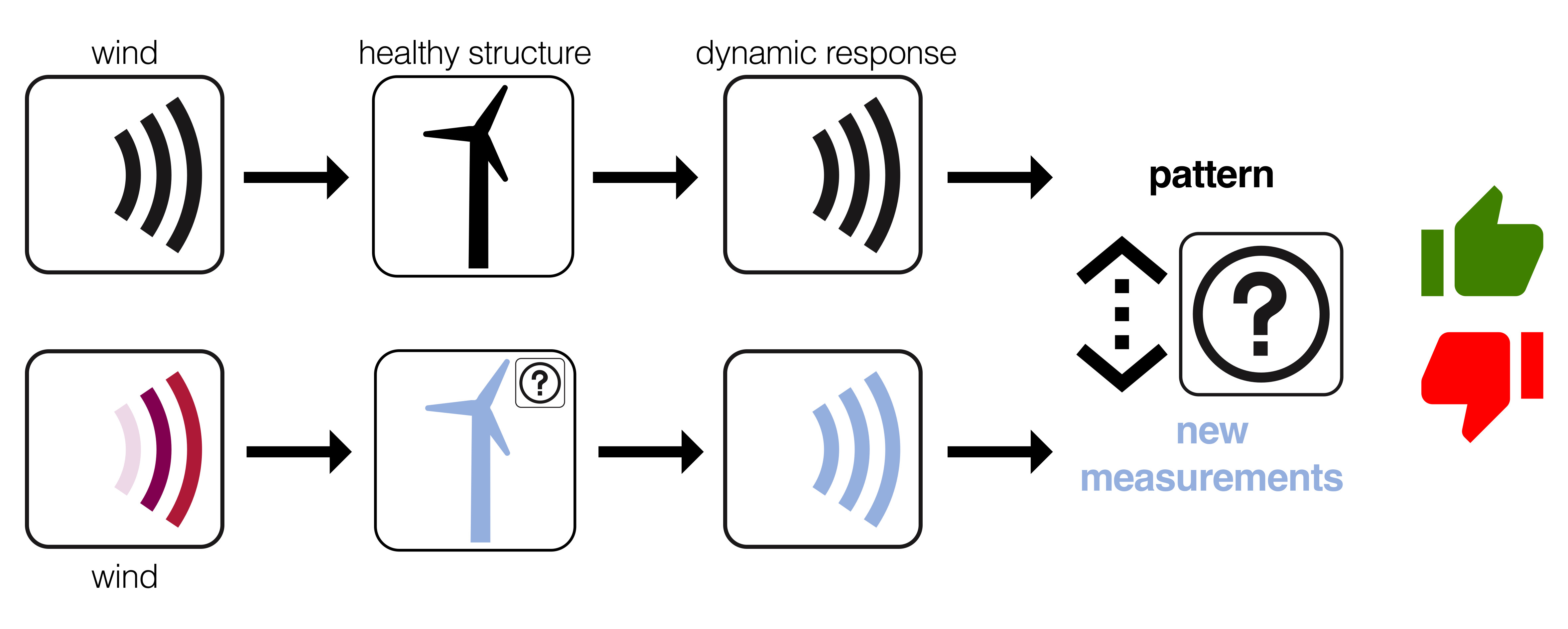
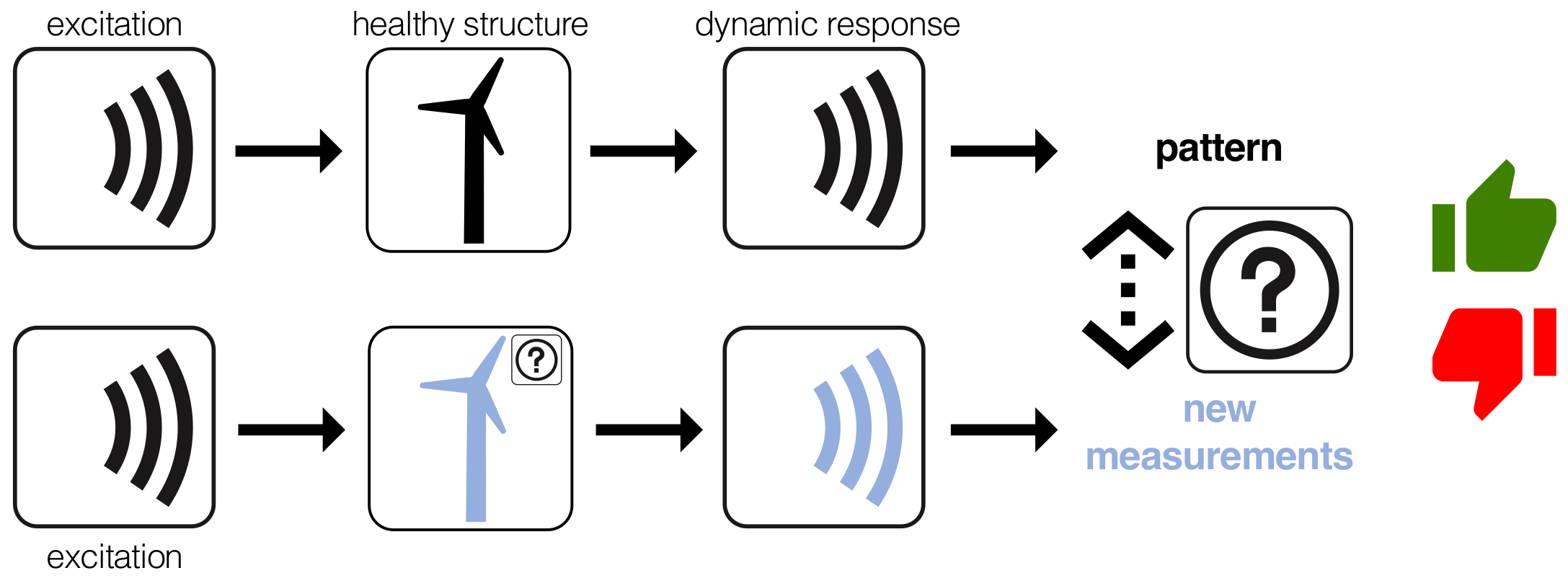
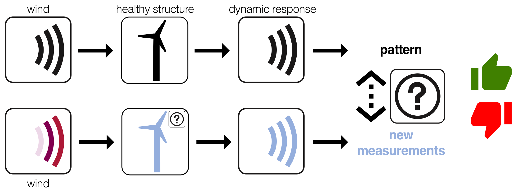
In structural health monitoring, a standard approach is the so-called vibration-based monitoring. It is based on the fact that a structural damage will alter the dynamic response of the structure, see Figure 1. In this approach, the structure to diagnose is excited by a prescribed and known signal. However, in the WT on-line monitoring, the vibration is caused by the wind, which is an stochastic unknown signal, see Figure 2. In this work, the obtained results given in Section 4 show that a change in the behavior of the overall system is detected by the proposed strategy even with a distinct (unkown) excitation.

3.2. Data Driven Baseline Modeling Based on MPCA

MPCA is a simple extension of conventional PCA to handle data in multi-dimensional arrays [26,27]. A typical two-dimensional (2D) data matrix can be considered as a two-way array, with experiments and variables (or discretization instant times) forming the two different ways. In some applications, it is necessary to extend this scheme to multiway arrays, for instance if in different experimental trials, several sensors are measuring at different time instants. MPCA is equivalent to performing ordinary PCA to an unfolded version of the original multiway array. According to Westerhuis et al. [28], there are six possible ways of unfolding a three-way data matrix. Out of the six possible unfolded matrices, in this paper we have considered type E with respect to the classification given by Ruiz et al. [29]. For the sake of clarity, in this paper, data is collected and arranged in an already unfolded matrix as it will be detailed in the posterior paragraphs.

The multiway PCA modeling in this paper starts by considering a healthy WT and measuring a sensor during $(nL-1)\Delta$ seconds, where both n and L are natural numbers and $\Delta$ is the corresponding sampling time. The discretized measures of the sensor can be arranged to form a vector of real values

$$\begin{array}{c}\hfill \left(\begin{array}{ccccccccccccc}{x}_{11}& x_{12}& \cdots & x_{1L}& x_{21}& x_{22}& \cdots & x_{2L}& \cdots & x_{n1}& x_{n2}& \cdots & x_{nL}\end{array}\right)\in {\mathbb{R}}^{nL}\end{array}$$

(1)

where $x_{ij}\in \mathbb{R},i=1,\dots ,n,j=1,\dots ,L$ is the measure of the sensor at time $\left((i-1)L+(j-1)\right)\Delta$ seconds. The $nL-$dimensional vector in Equation (1) can be rewritten as a matrix as follows:

$$\begin{array}{c}\hfill \left(\begin{array}{cccc}{x}_{11}& x_{12}& \cdots & x_{1L}\\ ⋮& ⋮& \ddots & ⋮\\ x_{i1}& x_{i2}& \cdots & x_{iL}\\ ⋮& ⋮& \ddots & ⋮\\ x_{n1}& x_{n2}& \cdots & x_{nL}\end{array}\right)\in {\mathcal{M}}_{n\times L}\left(\mathbb{R}\right)\end{array}$$

(2)

where ${\mathcal{M}}_{n\times L}\left(\mathbb{R}\right)$ represents the real vector space of $n\times L$ matrices. It is worth noting that L is the number of columns of the matrix in Equation (2) and n is the number of rows of the same matrix. The overall performance of the condition monitoring system is affected by the particular choice of n and L as is discussed on [30]. In a more general case, when the measures come from $N\in \mathbb{N}$ sensors, the assembled data can be disposed in matrix form as in Equation (2). Finally, for each sensor, the matrices in Equation (2) are concatenated to create a larger matrix $\mathbf{X}\in {\mathcal{M}}_{n\times (N·L)}$ as follows:

$$\begin{array}{cc}\hfill \mathbf{X}& =\left(\begin{array}{cccc}{x}_{11}^1& x_{12}^1& \cdots & x_{1L}^1\\ ⋮& ⋮& \ddots & ⋮\\ x_{i1}^1& x_{i2}^1& \cdots & x_{iL}^1\\ ⋮& ⋮& \ddots & ⋮\\ x_{n1}^1& x_{n2}^1& \cdots & x_{nL}^1\end{array}\left|\begin{array}{ccc}{x}_{11}^2& \cdots & x_{1L}^2\\ ⋮& \ddots & ⋮\\ x_{i1}^2& \cdots & x_{iL}^2\\ ⋮& \ddots & ⋮\\ x_{n1}^2& \cdots & x_{nL}^2\end{array}\right|\begin{array}{c}\cdots \\ \ddots \\ \cdots \\ \ddots \\ \cdots \end{array}|\begin{array}{ccc}{x}_{11}^N& \cdots & x_{1L}^N\\ ⋮& \ddots & ⋮\\ x_{i1}^N& \cdots & x_{iL}^N\\ ⋮& \ddots & ⋮\\ x_{n1}^N& \cdots & x_{nL}^N\end{array}\right)\hfill \\ & =(\underset{{\mathbf{X}}^1}{\underbrace{v_1|v_2|\cdots |v_L}}|\underset{{\mathbf{X}}^2}{\underbrace{v_{L+1}|\cdots |v_{2L}}}|\cdots |\underset{{\mathbf{X}}^N}{\underbrace{v_{(N-1)L+1}|\cdots |v_{N·L}}})\hfill \\ & =\left(\begin{array}{ccccccc}{\mathbf{X}}^1& |& {\mathbf{X}}^2& |& \cdots & |& {\mathbf{X}}^N\end{array}\right)\in {\mathcal{M}}_{n\times (N·L)}\left(\mathbb{R}\right)\hfill \end{array}$$

(3)

Given a generic element $x_{ij}^k$ of matrix $\mathbf{X}$, the superindex $k\in \{1,\dots ,N\}$ indicates the number of sensor. As a summary, matrix $\mathbf{X}\in {\mathcal{M}}_{n\times (N·L)}\left(\mathbb{R}\right)$ in Equation (3) includes the measures that come from N sensors at $nL$ discretization time instants. More precisely, the generic row vector

$$\begin{array}{c}\hfill x_i^T=\mathbf{X}(i,:)\in {\mathbb{R}}^{N·L},i=1,\dots ,n\end{array}$$

(4)

contains the measures from all the sensors at time instants $\left(\right(i-1)L+(j-1\left)\right)\Delta$ seconds, $j=1,\dots ,L$. Equivalently, the generic column vector

$$\begin{array}{c}\hfill v_j=\mathbf{X}(:,j)\in {\mathbb{R}}^n,j=1,\dots ,N·L\end{array}$$

contains the measures from sensor number $⌈j/L⌉$ at time instants $\left(\right(i-1)L+(j-1\left)\right)\Delta$ seconds, $1=1,\dots ,n$, where $\lceil ·\rceil$ is the ceiling function.

The main goal of the subsequent sections is to build the multiway PCA model, that is, the square matrix $\mathbf{P}\in {\mathcal{M}}_{(N·L)\times (N·L)}\left(\mathbb{R}\right)$ that has to be used to project the raw data stored in matrix $\mathbf{X}$ with the corresponding matrix-to-matrix product:

$$\begin{array}{c}\hfill \mathbf{T}=\mathbf{XP}\in {\mathcal{M}}_{n\times (N·L)}\left(\mathbb{R}\right).\end{array}$$

(5)

where the covariance matrix of matrix $\mathbf{T}$ in Equation (5) will be a diagonal matrix.

Group Scaling (GS) vs. Mean-Centered Group Scaling (MCGS)

Matrix $\mathbf{X}$ in Equation (3) includes the measures that come from several sensors. Consequently, the magnitudes measured by these sensors may have different scales. Therefore, it is recommended to apply some kind of pre-processing to rescale the collected data [31,32]. This pre-processing step can be performed in several ways that mainly depend on how the collected data is disposed in a matrix. In this case, we present two different alternatives: group scaling (GS) and mean-centered group scaling (MCGS). In the first case (GS), the scaling is based on the mean and the standard deviation of all measurements of the sensor. More precisely, we define

$$\begin{array}{cc}\hfill {\mu }^k& ={\displaystyle \frac{1}{nL}}\sum _{i=1}^n\sum _{j=1}^L{x}_{ij}^k,k=1,2,\dots ,N\hfill \end{array}$$

(6)

$$\begin{array}{cc}\hfill {\sigma }^k& =\sqrt{\frac{1}{nL}\sum _{i=1}^n\sum _{j=1}^L{(x_{ij}^k-{\mu }^k)}^2},k=1,2,\dots ,N\hfill \end{array}$$

(7)

where ${\mu }^k$ and ${\sigma }^k$ are the mean and the standard deviation of all the elements in matrix ${\mathbf{X}}^k$, respectively. More precisely, ${\mu }^k$ and ${\sigma }^k$ are the mean and the standard deviation of all the measures of sensor k, respectively. Consequently, the elements $x_{ij}^k$ of matrix $\mathbf{X}$ would be scaled –using GS– to create a new matrix $\check{\mathbf{X}}={\mathbf{X}}_{\mathrm{GS}}=({\check{x}}_{ij}^k)$ as

$$\begin{array}{cc}\hfill {\check{x}}_{ij}^k& :=\frac{x_{ij}^k-{\mu }^k}{{\sigma }^k},i=1,\dots ,n,j=1,\dots ,L,k=1,\dots ,N.\hfill \end{array}$$

(8)

In the second case (MCGS) the mean of all measurements of the sensor at the same column is considered in the normalization. More precisely, we define

$$\begin{array}{cc}\hfill {\mu }_j^k& =\frac{1}{n}\sum _{i=1}^n{x}_{ij}^k,j=1,\dots ,L,k=1,2,\dots ,N\hfill \end{array}$$

(9)

where ${\mu }_j^k$ is the arithmetic mean of the measures located at the same column, that is, the mean of the n measures of sensor k in matrix ${\mathbf{X}}^k$ at time instants $\left((i-1)L+(j-1)\right)\Delta$ seconds, $i=1,\dots ,n$. Therefore, the elements $x_{ij}^k$ of matrix $\mathbf{X}$ would be scaled –using MCGS– to create a new matrix $\breve{\mathbf{X}}={\mathbf{X}}_{\mathrm{MCGS}}=({\breve{x}}_{ij}^k)$ as

$$\begin{array}{cc}\hfill {\breve{x}}_{ij}^k& :=\frac{x_{ij}^k-{\mu }_j^k}{{\sigma }^k},i=1,\dots ,n,j=1,\dots ,L,k=1,\dots ,N.\hfill \end{array}$$

(10)

where ${\sigma }^k$ is defined as in Equation (7) using ${\mu }^k$ as in Equation (6). The arithmetic mean of each column vector in the scaled matrix $\breve{\mathbf{X}}$ can be calculated as

$$\begin{array}{cc}\hfill \frac{1}{n}\sum _{i=1}^n{\breve{x}}_{ij}^k& =\frac{1}{n}\sum _{i=1}^n\frac{x_{ij}^k-{\mu }_j^k}{{\sigma }^k}=\frac{1}{n{\sigma }^k}\sum _{i=1}^n\left(x_{ij}^k-{\mu }_j^k\right)\hfill \end{array}$$

(11)

$$\begin{array}{c}=\frac{1}{n{\sigma }^k}\left[\left(\sum _{i=1}^n{x}_{ij}^k\right)-n{\mu }_j^k\right]\hfill \end{array}$$

(12)

$$\begin{array}{c}=\frac{1}{n{\sigma }^k}\left(n{\mu }_j^k-n{\mu }_j^k\right)=0\hfill \end{array}$$

(13)

The scaled matrix $\breve{\mathbf{X}}$, whose elements are defined in Equation (10), is a mean-centered matrix. Taking advantage of this mean-centered property, the covariance matrix of matrix $\breve{\mathbf{X}}$ in Equation (10) can be simply computed as a matrix-to-matrix multiplication of both $\breve{\mathbf{X}}$ and its transpose. Indeed, the covariance matrix is computed as:

$${\mathbf{C}}_{\breve{\mathbf{X}}}=\frac{1}{n-1}{\breve{\mathbf{X}}}^T\breve{\mathbf{X}}\in {\mathcal{M}}_{(N·L)\times (N·L)}\left(\mathbb{R}\right)$$

(14)

Therefore, and since the calculation of the covariance matrix plays an important role in the application that we present in this paper, the Mean-Centered Group Scaling (MCGS) is the method that we have selected for the normalization. Throughout the rest of this work, matrix $\breve{\mathbf{X}}$, whose elements are defined in Equation (10), is renamed as simply $\mathbf{X}$.

The multiway PCA model is characterized by the eigenvectors $p_j,j=1,\dots ,N·L$—also called proper vectors or latent vectors—and the eigenvalues ${\lambda }_j,j=1,\dots ,N·L$—also called proper values or latent roots—of the covariance matrix in Equation (14) as follows:

$${\mathbf{C}}_{\mathbf{X}}\mathbf{P}=\mathbf{P}\mathsf{\Lambda }$$

(15)

where

$$\begin{array}{cc}\hfill \mathbf{P}& =\left(p_1|p_2|\cdots |p_{N·L}\right)\in {\mathcal{M}}_{N·L\times N·L}\left(\mathbb{R}\right)\hfill \end{array}$$

(16)

$$\begin{array}{cc}\hfill \mathsf{\Lambda }& =\left({\mathsf{\Lambda }}_{ij}\right)\in {\mathcal{M}}_{N·L\times N·L}\left(\mathbb{R}\right)\hfill \end{array}$$

(17)

and

$$\begin{array}{cc}\hfill {\mathsf{\Lambda }}_{jj}& ={\lambda }_j,j=1,\dots ,N·L\hfill \end{array}$$

(18)

$$\begin{array}{cc}\hfill {\mathsf{\Lambda }}_{ij}& =0,i,j=1,\dots ,N·L,i\ne j\hfill \end{array}$$

(19)

In Equations (16) and (18) it is assumed that the eigenvalues are organized in descending order with respect to their absolute values, that is,

$$\begin{array}{c}\hfill |{\lambda }_i|\ge |{\lambda }_{i+1}|,i=1,\dots ,N·L-1\end{array}$$

(20)

The eigenvector $p_1$—corresponding to ${\lambda }_1$—is called the first principal component. Similarly, the eigenvector $p_2$—corresponding to ${\lambda }_2$—is called the second principal component, and so on.

Matrix $\mathbf{T}$ in Equation (5) is the projected or transformed matrix onto the principal component space –also called score matrix.

If we consider a reduced number

$$\begin{array}{c}\hfill \ell <N·L\end{array}$$

(21)

of principal components, a simplified multiway PCA model is then built:

$$\begin{array}{c}\hfill \widehat{\mathbf{P}}=\left(p_1|p_2|\cdots |p_{\ell }\right)\in {\mathcal{M}}_{N·L\times \ell }\left(\mathbb{R}\right)\end{array}$$

(22)

3.3. Condition Monitoring Strategy Based on MSHT

The WT that has to be diagnosed is subjected to a wind turbulence that is changing as it is illustrated in Section 2 and Section 3.2. If we consider that the measures come from $N\in \mathbb{N}$ sensors during $(\nu L-1)\Delta$ seconds, an assembled data matrix $\mathbf{Y}$ is constructed similarly as in Equation (3):

$$\begin{array}{cc}\hfill \mathbf{Y}& =\left(\begin{array}{cccc}{y}_{11}^1& y_{12}^1& \cdots & y_{1L}^1\\ ⋮& ⋮& \ddots & ⋮\\ y_{i1}^1& y_{i2}^1& \cdots & y_{iL}^1\\ ⋮& ⋮& \ddots & ⋮\\ y_{\nu 1}^1& y_{\nu 2}^1& \cdots & y_{\nu L}^1\end{array}\left|\begin{array}{ccc}{y}_{11}^2& \cdots & y_{1L}^2\\ ⋮& \ddots & ⋮\\ y_{i1}^2& \cdots & y_{iL}^2\\ ⋮& \ddots & ⋮\\ y_{\nu 1}^2& \cdots & y_{\nu L}^2\end{array}\right|\begin{array}{c}\cdots \\ \ddots \\ \cdots \\ \ddots \\ \cdots \end{array}|\begin{array}{ccc}{y}_{11}^N& \cdots & y_{1L}^N\\ ⋮& \ddots & ⋮\\ y_{i1}^N& \cdots & y_{iL}^N\\ ⋮& \ddots & ⋮\\ y_{\nu 1}^N& \cdots & y_{\nu L}^N\end{array}\right)\in {\mathcal{M}}_{\nu \times (N·L)}\left(\mathbb{R}\right)\hfill \\ & =(\underset{{\mathbf{Y}}^1}{\underbrace{w_1|w_2|\cdots |w_L}}|\underset{{\mathbf{Y}}^2}{\underbrace{w_{L+1}|\cdots |w_{2L}}}|\cdots |\underset{{\mathbf{Y}}^N}{\underbrace{w_{(N-1)L+1}|\cdots |w_{N·L}}})\hfill \\ & =\left(\begin{array}{ccccccc}{\mathbf{Y}}^1& |& {\mathbf{Y}}^2& |& \cdots & |& {\mathbf{Y}}^N\end{array}\right)\in {\mathcal{M}}_{n\times (N·L)}\left(\mathbb{R}\right)\hfill \end{array}$$

(23)

It is very important to mention that, as stated by Pozo and Vidal [33], the number of rows of matrix $\mathbf{Y}$ should not be necessarily equal to the number of rows of $\mathbf{X}$ in Equation (3). However, the number of columns must agree.

The assembled data in matrix $\mathbf{Y}$ in Equation (23) is first scaled to create a matrix $\breve{\mathbf{Y}}=({\breve{y}}_{ij}^k)$ as in Equation (10):

$$\begin{array}{cc}\hfill {\breve{y}}_{ij}^k& :=\frac{y_{ij}^k-{\mu }_j^k}{{\sigma }^k},i=1,\dots ,\nu ,j=1,\dots ,L,k=1,\dots ,N,\hfill \end{array}$$

(24)

where ${\sigma }^k$ and ${\mu }_j^k$ are the values that have already been computed in Equations (7) and (9), respectively, with respect to $\mathbf{X}$ in Equation (3). After this pre-processing step, the scores associated with each row vector

$$\begin{array}{c}\hfill r^i=\breve{\mathbf{Y}}(i,:)\in {\mathbb{R}}^{N·L},i=1,\dots ,\nu \end{array}$$

(25)

are calculated through a vector-to-matrix multiplication:

$$\begin{array}{c}\hfill t^i=r^i·\widehat{\mathbf{P}}\in {\mathbb{R}}^{\ell },i=1,\dots ,\nu \end{array}$$

(26)

where matrix $\widehat{\mathbf{P}}$ is the simplified multiway PCA model in Equation (22).

Let $\{{\mathbf{e}}_1,{\mathbf{e}}_2,\dots ,{\mathbf{e}}_{\ell }\}\subset {\mathbb{R}}^{\ell }$ be the canonical basis. For each row vector $r^i$, the scalar

$$\begin{array}{c}\hfill t_1^i=t^i·{\mathbf{e}}_1\in \mathbb{R}\end{array}$$

(27)

is called the first score. Similarly, the scalar

$$\begin{array}{c}\hfill t_2^i=t^i·{\mathbf{e}}_2\in \mathbb{R}\end{array}$$

(28)

is called the second score, and so on.

If more than one score is considered at the same time, we can build and s-dimensional vector as

$$\begin{array}{c}\hfill {\mathbf{t}}_s^i={\left[\begin{array}{cccc}{t}_1^i& t_2^i& \cdots & t_s^i\end{array}\right]}^T\in {\mathbb{R}}^s,s\le \ell .\end{array}$$

(29)

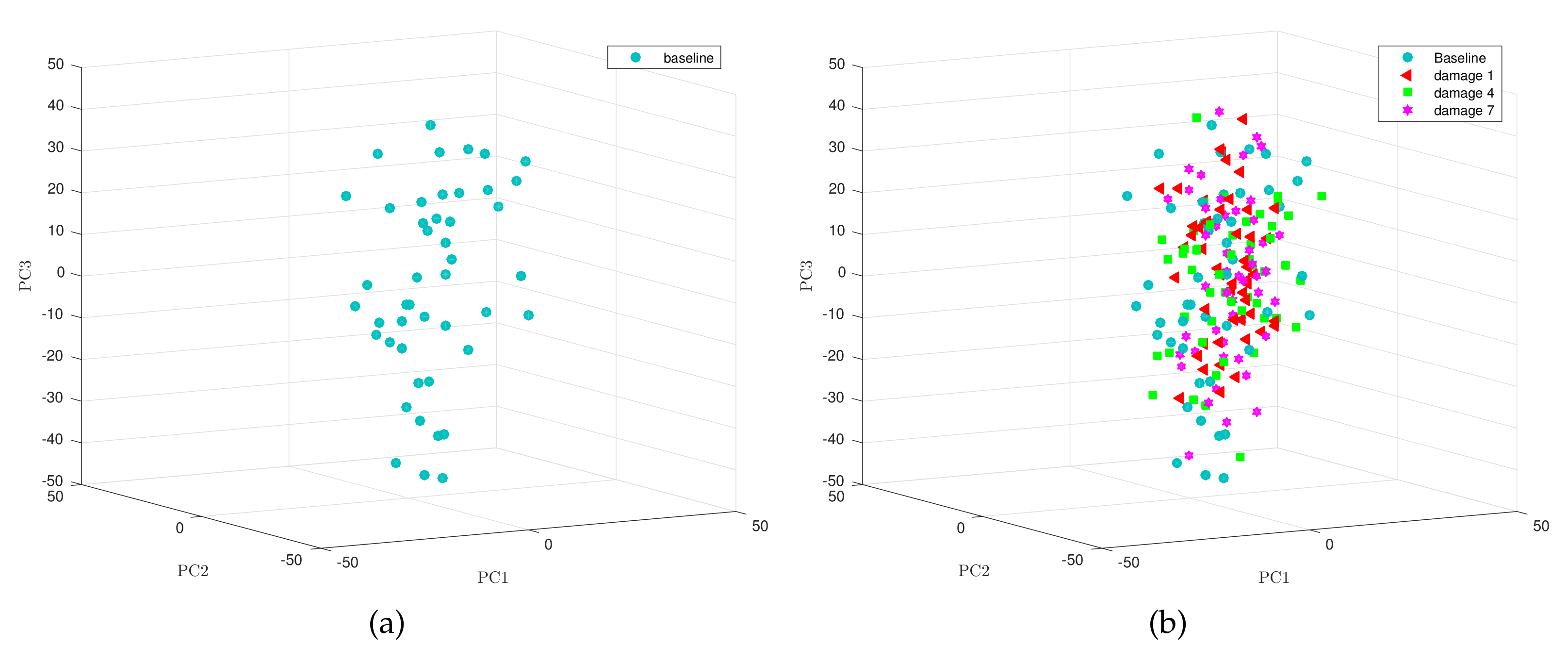
Vector ${\mathbf{t}}_s^i$ in Equation (29) can be seen as an $s-$dimensional random vector [16]. As an interesting example, we have depicted in Figure 3 some 50 element samples of the three dimensional random vector

$$\begin{array}{c}\hfill {\mathbf{t}}_3^i={\left[\begin{array}{ccc}{t}_1^i& t_2^i& t_3^i\end{array}\right]}^T,i=1,\dots ,50\end{array}$$

(30)

One corresponds to the baseline sample (Figure 3a) and the other is referred to faults 1, 4 and 7 (Figure 3b).

Testing a Multivariate Mean Vector

In order to classify the WT state (healthy or faulty) it is needed to decide if the distribution of the multivariate random samples from the WT to be monitorized is related to the distribution of the baseline. To reach this goal, a test for the plausibility of a value for a normal population mean vector is carried out.

Let $s\in \mathbb{N}$ be the number of principal components to be employed. We assume that the baseline projection is a sample of a multivariate random variable following a multivariate normal distribution (MVND) with known population mean vector, ${\mathbf{\mu }}_{\mathrm{h}}\in {\mathbb{R}}^s$, and known variance-covariance matrix, $\mathsf{\Sigma }\in {\mathcal{M}}_{s\times s}\left(\mathbb{R}\right)$. Finally, we also assume that the sample to be monitorized follows a MVND with unknown multivariate mean vector, ${\mathbf{\mu }}_{\mathrm{c}}\in {\mathbb{R}}^s$, and known variance-covariance matrix, $\mathsf{\Sigma }\in {\mathcal{M}}_{s\times s}\left(\mathbb{R}\right)$.

We need to decide whether a given s-dimensional vector, ${\mathbf{\mu }}_{\mathrm{c}}$, is a plausible value for the mean of a MVND , $N_s({\mathbf{\mu }}_{\mathrm{h}},\mathsf{\Sigma })$. Thus, the next hypothesis test follows

$$\begin{array}{cc}\hfill H_0& :{\mathbf{\mu }}_{\mathrm{c}}={\mathbf{\mu }}_{\mathrm{h}}\mathrm{versus}\hfill \\ \hfill H_1& :{\mathbf{\mu }}_{\mathrm{c}}\ne {\mathbf{\mu }}_{\mathrm{h}}.\hfill \end{array}$$

Here, the null hypothesis is ‘the sample of the WT to be monitorized is distributed as the baseline’. Thus, when the null hypothesis is accepted, the current WT is classified as healthy. Otherwise, a fault is present in the WT.

The hypothesis test is grounded on the Hotelling’s $T^2$ statistic. When a sample of size $\nu \in \mathbb{N}$ is taken from a MVND $N_s({\mathbf{\mu }}_{\mathrm{h}},\mathsf{\Sigma })$, the random variable

$$\begin{array}{c}\hfill T^2=\nu {\left(\overline{\mathbf{X}}-{\mathbf{\mu }}_{\mathrm{h}}\right)}^T{\mathbf{S}}^{-1}\left(\overline{\mathbf{X}}-{\mathbf{\mu }}_{\mathrm{h}}\right)\end{array}$$

is distributed as

$$\begin{array}{c}\hfill T^2\hookrightarrow \frac{(\nu -1)s}{\nu -s}{F}_{s,\nu -s},\end{array}$$

where $F_{s,\nu -s}$ denotes a random variable with an F-distribution with s and $\nu -s$ degrees of freedom, $\overline{\mathbf{X}}$ is the sample vector mean as a multivariate random variable; and $\frac{1}{n}\mathbf{S}\in {\mathcal{M}}_{s\times s}\left(\mathbb{R}\right)$ is the estimated covariance matrix of $\overline{\mathbf{X}}$.

At a given level of significance, $\alpha$, we reject $H_0$ when the observed

$$\begin{array}{c}\hfill t_{\mathrm{obs}}^2=\nu {\left(\overline{\mathbf{x}}-{\mathbf{\mu }}_{\mathrm{h}}\right)}^T{\mathbf{S}}^{-1}\left(\overline{\mathbf{x}}-{\mathbf{\mu }}_{\mathrm{h}}\right)\end{array}$$

is greater than $\frac{(\nu -1)s}{\nu -s}{F}_{s,\nu -s}\left(\alpha \right)$, where $F_{s,\nu -s}\left(\alpha \right)$ is the upper $\left(100\alpha \right)$th percentile of the $F_{s,\nu -s}$ distribution. Namely, the quantity $t_{\mathrm{obs}}^2$ is the fault indicator and the test is:

$$\begin{array}{cc}\hfill t_{\mathrm{obs}}^2\le \frac{(\nu -1)s}{\nu -s}{F}_{s,\nu -s}\left(\alpha \right)& ⟹\mathrm{Fail}\mathrm{to}\mathrm{reject}{H}_0,\hfill \end{array}$$

(31)

$$\begin{array}{cc}\hfill t_{\mathrm{obs}}^2>\frac{(\nu -1)s}{\nu -s}{F}_{s,\nu -s}\left(\alpha \right)& ⟹\mathrm{Reject}{H}_0,\hfill \end{array}$$

(32)

where $F_{s,\nu -s}\left(\alpha \right)$ is such that

$$\begin{array}{c}\hfill \mathbb{P}\left(F_{s,\nu -s}>F_{s,\nu -s}\left(\alpha \right)\right)=\alpha ,\end{array}$$

where $\mathbb{P}$ is a probability measure.

In a nutshell, we accept the null hypothesis if $t_{\mathrm{obs}}^2\le \frac{(\nu -1)s}{\nu -s}{F}_{s,\nu -s}\left(\alpha \right)$, thus showing that the WT is healthy. Otherwise, the alternative hypothesis is accepted, thus leading to a faulty WT diagnostic.

4. Simulation Results

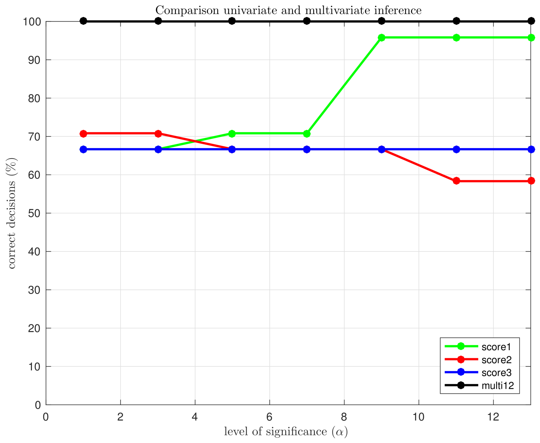
The results of the condition monitoring strategy are presented and grouped in three different subsections. Section 4.2 includes the quantity of samples that are correctly classified and the number of missing faults and false alarms. Section 4.3 and Section 4.4 present the results as a percentage. On one hand, Section 4.3 comprises both the specificity and the sensitivity, together with the false-positive and the false-negative rates. On the other hand, Section 4.4 contains the true rate of both false positives and false negatives. Finally, Section 4.5 includes a discussion on the level of significance $\alpha$ of the test. Based on that discussion, in the multivariate case, it will be seen that the level of significance can be reduced—therefore reducing the ratio of false alarms—without affecting the overall performance of the fault detection strategy.

4.1. Multivariate Normality

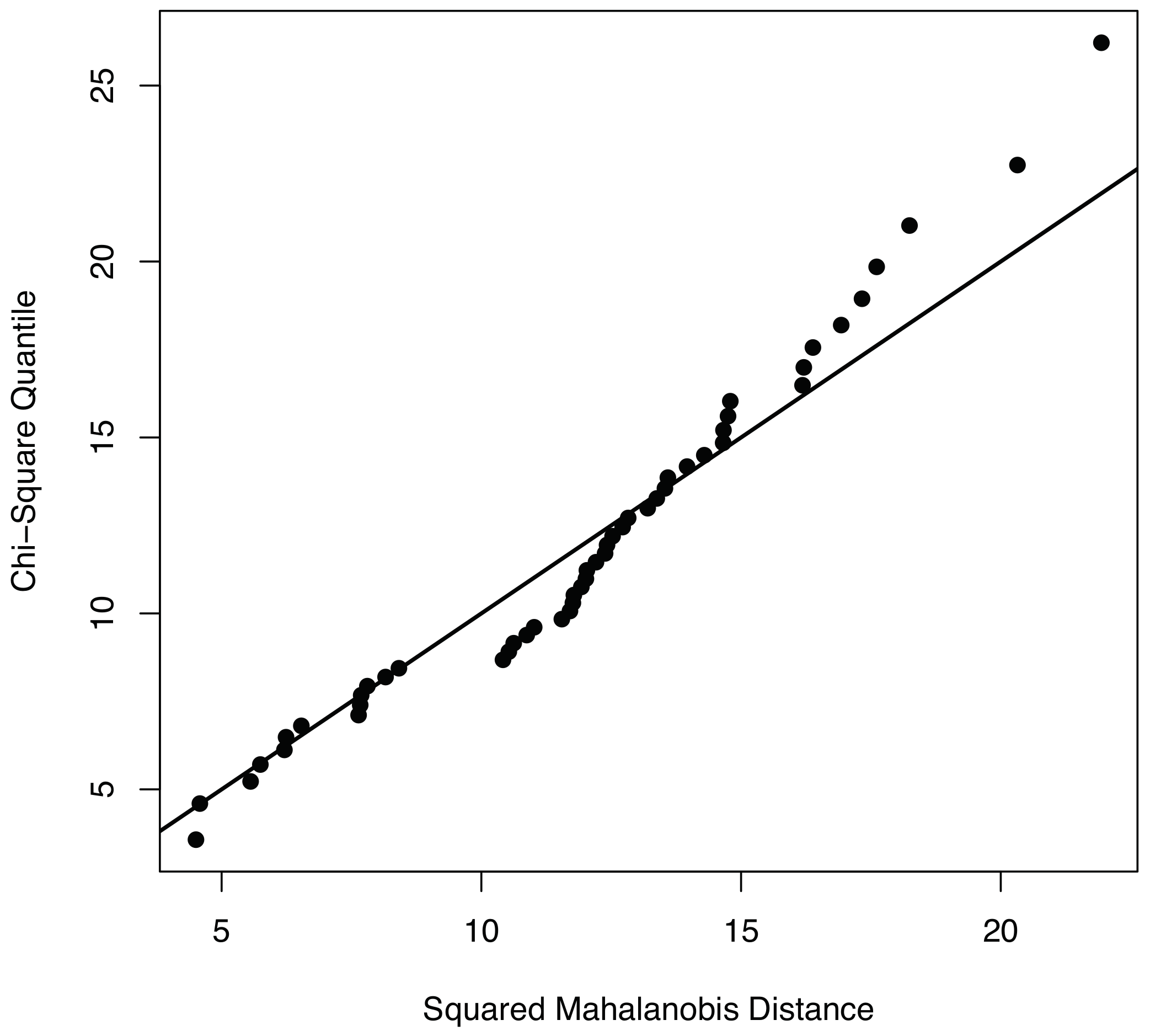
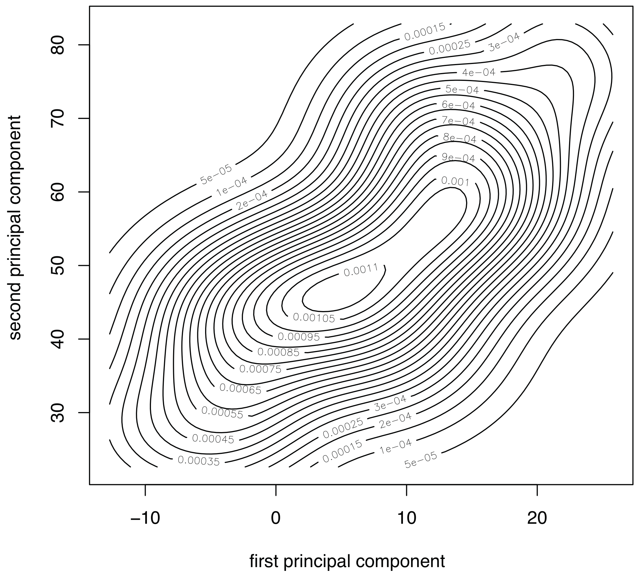
To properly apply the condition monitoring strategy described in Section 3, and more precisely, the multivariate hypothesis testing outlined in Section 3.3.1, measured data should be compatible with a multivariate normal distribution. To visually show the normality of the data used to validate the condition monitoring strategy, we use both the Q–Q plots and the contour plots. With respect to the Q–Q plots, it can be observed in Figure 4 that the points of the sample related to fault number 1—using the first twelve principal components—are distributed closely following the bisectrix, thus indicating the multivariate normality of the data. Moreover, a contour plot for the data we consider in this work is given in Figure 5. More accurately, Figure 5 represents the contour plot for the sample corresponding to fault number 4, and principal components 1 and 2. The contour lines are similar to ellipses of a normal bivariate distribution that means that the distribution in this case is, again, consistent with the assumption of multinormality. Although the graphical approaches can be useful to visually show the normality, a formal test for multivariate normality should be applied. However, since there is no single most powerful test it is recommended to perform several tests to assess the multivariate normality. Consequently, we will consider the three most widely used normality tests:

(i)

Mardia’s;

(ii)

Henze-Zirkler’s; and

(iii)

Royston’s

multivariate normality tests. A brief explanation of these methods can be found in [16].

Table 3. Results of the normality tests when considering the first two principal components, the first seven principal components and the first twelve principal components. “−” means that all the tests rejected multivariate normality while “+” means that at least one test indicated multivariate normality. In this last case, the subindex shows the tests that indicated multinormality: 1 (Mardia’s test), 2 (Henze–Zirkler’s test), or 3 (Royston’s test).

Fault Number	PC 1 to 2	PC 1 to 7	PC 1 to 12
1	${+}_{1,2,3}$	${+}_{1,2,3}$	${+}_{1,2,3}$
2	${+}_{1,2,3}$	${+}_{1,2,3}$	${+}_{1,2,3}$
3	${+}_{1,2,3}$	${+}_{1,2,3}$	${+}_{1,2,3}$
4	${+}_{1,2,3}$	${+}_{1,2,3}$	${+}_{2,3}$
5	${+}_{1,2,3}$	${+}_{2,3}$	${+}_{1,3}$
6	${+}_{1,2,3}$	${+}_{2,3}$	${+}_3$
7	${+}_{1,2,3}$	${+}_{2,3}$	${+}_{1,2,3}$
8	${+}_{1,2,3}$	${+}_{1,2,3}$	${+}_{1,2,3}$

summarizes the results of the three normality tests when considering the first two principal components, the first seven principal components and the first twelve principal components.

4.2. Type I and Type II Errors

The condition monitoring strategy presented in Section 3 is carried out considering a total of 24 samples of $\nu =50$ elements each, according to the following distribution:

• 16 samples of a healthy wind turbine; and
• 8 samples of a faulty wind turbine (one sample for each one of the different fault scenarios described in Table 2).

All samples are obtained with different wind data sets with turbulence intensity set to $10\%$ and generated with TurbSim [34]. The generated wind data has the following characteristics: Kaimal turbulence model, logarithmic profile wind type, mean speed of $18.2$ m/s simulated at hub height, and a roughness factor of $0.01$ m. Each sample of $\nu =50$ elements comes from the measures obtained from the $N=13$ sensors detailed in Table 1 during $(\nu ·L-1)\Delta =312.4875$ s, where $L=500$ and the sampling time is $\Delta =0.0125$ s. This sampling time represents a sampling ratio of 80 Hz. Although Lind et al. [14] propose a more realistic sampling ratio of 1 Hz, they also agree with the fact that a mixed system, combining SCADA and conventional high frequency sensors is expected in the near future. The measures are arranged in a $\nu \times (N·L)$ matrix $\mathbf{Y}$ as in Equation (23). As it can be observed, the number of rows of matrix $\mathbf{Y}$ equals the number of elements in the sample. Therefore, the first element of the sample is the projection of the first row of matrix $\mathbf{Y}$ into one or more principal components; the second element of the sample is the projection of the second row of matrix $\mathbf{Y}$ into one or more principal components, and so on. When the projection is performed into a single principal component, the sample is then equivalent to a set of real numbers. However, when the projection is performed into more than one principal component, the sample can be considered as a set of $s-$dimensional vectors, where $s\in \mathbb{N}$ is the number of principal components that are considered jointly. One of the main contributions of this paper is that the condition monitoring strategy is based on multivariate statistical hypothesis testing applied to this set of $s-$dimensional vectors.

The main goal of this section is to show the benefits of the multivariate statistical hypothesis testing with respect to the univariate case. To this end, we present the results when the measured data is projected into the first, the second and the third principal component, separately. Basically, when the sample is a set of real numbers, the condition monitoring is based on the univariate hypothesis testing presented in [33]. These results will be compared with a new condition monitoring strategy where the measured data is projected into: (i) the first and the second principal component, jointly; (ii) the seven first principal components, jointly; and (iii) the twelve principal components, jointly.

These 24 samples plus the baseline sample of $n=50$ elements are used to test for the equality of means (in the univariate case) or to test for the plausibility of a value for a normal population mean vector (in the multivariate case), with a level of significance $\alpha =10\%$ in both cases. Each sample of $\nu =50$ elements is categorized as follows:

(i)

number of samples from the healthy wind turbine (healthy sample) which were classified by the hypothesis test as ‘healthy’ (fail to reject $H_0$ / accept $H_0$);

(ii)

faulty sample classified by the test as ‘faulty’ (reject $H_0$ / accept $H_1$);

(iii)

samples from the faulty structure (faulty sample) classified as ‘healthy’; and

(iv)

faulty sample classified as ‘faulty’.

The results –organized according to the scheme in

Table 4. Guide for the presentation of the results in Table 5.

	Healthy Sample (${\mathit{H}}_0$)	Faulty Sample (${\mathit{H}}_1$)
Accept $H_0$	Right decision	Missing fault (type II error)
Accept $H_1$	False alarm (type I error)	Right decision

– are presented in

Table 5. Categorization of the samples with respect to the presence or absence of a fault and the result of the test considering the first score, the second score, the third score (left); and scores 1 to 2 (jointly), scores 1 to 7 (jointly), and scores 1 to 12 (jointly) (right), when $\nu =50$ and $\alpha =10\%$.

	${\mathit{H}}_0$	${\mathit{H}}_1$
Score 1
Accept $H_0$	16	1
Accept $H_1$	0	7
Score 2
Accept $H_0$	13	7
Accept $H_1$	3	1
Score 3
Accept $H_0$	16	8
Accept $H_1$	0	0
	${\mathit{H}}_0$	${\mathit{H}}_1$
Scores 1 to 2
Accept $H_0$	12	0
Accept $H_1$	4	8
Scores 1 to 7
Accept $H_0$	13	0
Accept $H_1$	3	8
Scores 1 to 12
Accept $H_0$	16	0
Accept $H_1$	0	8

. It can be stressed, from Table 5, that the sum of the columns is constant: 16 samples in the first column (healthy wind turbine) and 8 more samples in the second column (faulty wind turbine).

Table 5 includes the results using both the univariate hypothesis testing fault detection strategy developed in [33] (for the first, second and third score) and the multivariate hypothesis testing presented in this work (scores 1 to 2, 1 to 7 and 1 to 12, jointly). It is worth noting that, for a fixed level of significance $\alpha =10\%$, all decisions are correct when the first twelve scores are considered jointly. In the other cases, two kinds of misclassifications are presented: (i) type I error; and (ii) type II error. The type I error, also known as false positive or false alarm, occurs when the wind turbine is working correctly but the condition monitoring strategy infers that there is some problem. The level of significance $\alpha$ is , at the same time, the probability of committing this type of error. Additionally, the type II error, also known as false negative or missing fault, appears when the wind turbine is not working properly but the strategy classifies it as healthy. The probability of committing this type of error is called $\gamma$. This value is closely related to the sensitivity of the test, as it will be seen in Section 4.3.

4.3. Sensitivity and Specificity

As in [33], two more statistical measures are considered to examine the efficiency of the test. On one hand, the sensitivity—or the power of the test—is defined as the fraction of samples from the faulty wind turbine that are correctly classified as such. On the other hand, the specificity of the test is defined as the fraction of samples from the healthy structure which are correctly classified. Both the specificity and the sensitivity can be expressed in terms of the level of significance $\alpha$ and the real number $\gamma$ defined in Section 4.2, as it is specified in

Table 6. Relationship between specificity and sensitivity, false-positive rate (FPR) and false-negative rate (FNR).

	Healthy Sample (${\mathit{H}}_0$)	Faulty Sample (${\mathit{H}}_1$)
Accept $H_0$	Specificity ($1-\alpha$)	FNR ($\gamma$)
Accept $H_1$	FPR ($\alpha$)	Sensitivity ($1-\gamma$)

.

The specificity and sensitivity of both the univariate hypothesis testing and the multivariate case with respect to the 24 samples—arranged as shown in Table 6—have been included in

Table 7. Sensitivity and specificity of the test considering the first score, the second score, the third score (left); and scores 1 to 2 (jointly), scores 1 to 7 (jointly), and scores 1 to 12 (jointly) (right), when $\nu =50$ and $\alpha =10\%$.

	${\mathit{H}}_0$	${\mathit{H}}_1$
Score 1
Accept $H_0$	1.00	0.12
Accept $H_1$	0.00	0.88
Score 2
Accept $H_0$	0.81	0.88
Accept $H_1$	0.19	0.12
Score 3
Accept $H_0$	1.00	1.00
Accept $H_1$	0.00	0.00
	${\mathit{H}}_0$	${\mathit{H}}_1$
Scores 1 to 2
Accept $H_0$	0.75	0.00
Accept $H_1$	0.25	1.00
Scores 1 to 7
Accept $H_0$	0.81	0.00
Accept $H_1$	0.19	1.00
Scores 1 to 12
Accept $H_0$	1.00	0.00
Accept $H_1$	0.00	1.00

.

For the univariate case, the results in Table 7 show that the average value of the sensitivity is $33.33\%$, which is far from the desired value of $100\%$. The average value of the specificity is $93.67\%$, which is very close to the expected value of $1-\alpha =90\%$. However, in the multivariate case, the average values of the sensitivity and the specificity are $100\%$ and $85.33\%$, respectively. Although the average specificity in the univariate case is slightly greater than the average specificity in the multivariate case, the sensitivity in the multivariate case is undoubtedly better than the sensitivity in the univariate case. The proposed methodology thus surpasses the performance of the fault detection strategy based on univariate hypothesis testing.

4.4. Reliability of the Results

Two more statistical measures that can be used to assess the performance of the proposed condition monitoring strategy are the true rate of false negatives and the true rate of false positives. These two measures—rooted in Bayes’ theorem [35]—are described in

Table 8. Relationship between the proportion of false negatives and false positives.

	Healthy Sample (${\mathit{H}}_0$)	Faulty Sample (${\mathit{H}}_1$)
Accept $H_0$	$\mathbb{P}\left(H_0\right|\mathrm{accept}{H}_0)$	$\begin{array}{c}\mathrm{true}\mathrm{rate}\mathrm{of}\mathrm{false}\mathrm{negatives}\hfill \\ \mathbb{P}\left(H_1\right|\mathrm{accept}{H}_0)\hfill \end{array}$
Accept $H_1$	$\begin{array}{c}\mathrm{true}\mathrm{rate}\mathrm{of}\mathrm{false}\mathrm{positives}\hfill \\ \mathbb{P}\left(H_0\right|\mathrm{accept}{H}_1)\hfill \end{array}$	$\mathbb{P}\left(H_1\right|\mathrm{accept}{H}_1)$

. More precisely, the true rate of false negatives is the fraction of samples from the faulty wind turbine that have been mistakenly identified as healthy. Contrarily, the true rate of false positives is the fraction of sample from the healthy wind turbine that have been mistakenly identified as faulty.

For the univariate case, the results in

Table 9. True rate of false negatives and true rate of false positives of the test considering the first score, the second score, the third score (left); and scores 1 to 2 (jointly), scores 1 to 7 (jointly), and scores 1 to 12 (jointly) (right), when $\nu =50$ and $\alpha =10\%$.

	${\mathit{H}}_0$	${\mathit{H}}_1$
Score 1
Accept $H_0$	0.94	0.06
Accept $H_1$	0.00	1.00
Score 2
Accept $H_0$	0.65	0.35
Accept $H_1$	0.75	0.25
Score 3
Accept $H_0$	0.67	0.33
Accept $H_1$	0.00	0.00
	${\mathit{H}}_0$	${\mathit{H}}_1$
Scores 1 to 2
Accept $H_0$	1.00	0.00
Accept $H_1$	0.33	0.67
Scores 1 to 7
Accept $H_0$	1.00	0.00
Accept $H_1$	0.27	0.73
Scores 1 to 12
Accept $H_0$	1.00	0.00
Accept $H_1$	0.00	1.00

show that the average value of the true rate of false negatives is $24.67\%$, which is far from the desired value of $0\%$. The average value of the true rate of false positives is $25.00\%$. However, in the multivariate case, the average values of the true rate of false negatives and the true rate of false positives are $0.00\%$ and $20.00\%$, respectively. Although the average value of the true rate of false positives in the univariate case is similar to the same magnitude in the multivariate case, the true rate of false negatives in the multivariate case is clearly better. Once more the proposed methodology outperforms the fault detection strategy based on univariate hypothesis testing.

4.5. Discussion on the Level of Significance

The performance of the proposed condition monitoring strategy through principal component analysis and multivariate statistical hypothesis testing depends on:

• the number $\nu \in \mathbb{N}$ of elements of each sample;
• the number $L\in \mathbb{N}$ of columns of each sub-matrix—corresponding to a sensor—in matrix $\mathbf{Y}$ in Equation (23).
• the number $s\in \mathbb{N}$ of principal components considered jointly; and
• the level of significance $\alpha \in [0,1]$ of the multivariate hypothesis testing.

The effect on the overall performance of the proposed method of the choice of $\nu$ and L is exhaustively discussed on [30] for the univariate case though the results can be easily extrapolated to the multivariate case. The influence of the number s of principal components considered jointly is also accurately examined in [16]. As it is expected, the more number of principal components are considered, the better results are obtained.

The choice of the level of significance $\alpha$ is of an extreme importance too. Therefore, for the choice of $\alpha$, two considerations have to be taken into account:

• the level of significance $\alpha$ is the probability of committing a type I error (false alarm);
• type II errors (missing faults) should be reduced.

Consequently, a small level of significance is desired, but an excessively small level of significance would lead to a higher rate of missing faults. For that reason, the question is: how small the level of significance can be selected without affecting the rate of missing faults? In Figure 6 we have depicted the percentage of correct decisions using the multivariate hypothesis testing fault detection strategy with the first twelve principal components (jointly) and the univariate hypothesis testing, for the first, the second and the third principal components (separately), as a function of the level of significance $\alpha$. It can be clearly observed that, in the univariate case, if the level of significance is reduced from $\alpha =13\%$ to $\alpha =1\%$, the overall performance is degraded. However, in the multivariate case, the reduction of the level of significance—and thus the reduction of type I errors—does not affect the fault detection strategy, keeping the percentage of correct decisions at $100\%$.

5. Concluding Remarks

This paper presents a condition monitoring system for WTs based on conventional SCADA data. The results confirm the effectiveness of the methodology and its usefulness as a condition monitoring tool through the study of eight realistic different faults (covering actuators, and sensors) in different parts of the wind turbine following the WT fault detection benchmark proposed in [15].

One main contribution of this work is to show the benefits of the multivariate statistical hypothesis testing with respect to the univariate case, for PCA-based WT fault detection. Firstly, it is noteworthy that, for a fixed level of significance $\alpha =10\%$, all decisions are correct when the first twelve scores are considered jointly while in all the other studied cases misclassifications are present (missing faults and/or false alarms). Secondly, for the univariate case the average value of the sensitivity is only $33.33\%$ and the specificity is $93.67\%$ while for the multivariate case the average values are $100\%$ and $85.33\%$, respectively. Thirdly, for the univariate case, the average value of the true rate of false negatives is $24.67\%$ and the average value of the true rate of false positives is $25\%$ while for the multivariate case the average values are $0\%$ and $20\%$, respectively. Finally, in the univariate case, if the level of significance is reduced (from $\alpha =13\%$ to $\alpha =1\%$), the overall performance is degraded while in the multivariate case, the percentage of correct decisions is kept at $100\%$.

Ultimately, note that access to real SCADA datasets is often proprietary. Therefore, it is not accessible by the scientific community. However, in case experimental data sets could be fed to the proposed inference machine, two shortcomings would be encountered: the sampling time and the sensors measurement noise. With respect to the sampling time, in this work a 80 Hz sampling time is used while traditionally sampling for SCADA is 1Hz frequency or lower. However, as noted in [14] “a mixed system, combining SCADA data and conventional high frequency sensors is expected in the future”. With regard to the real measurement noise, the robustness of the proposed strategy is given by the multiway PCA used for pretreatment. Recall that PCA has the effect of concentrating much of the data into the first few principal components, which can usefully be captured by dimensionality reduction; while the later principal components may be dominated by noise, and so disposed of without great loss. Furthermore, to enhance the strategy in this respect, future work replacing PCA with robust PCA would be considered.

References

- Lindenberg, S.; Smith, B.; O’Dell, K.; Demeo, E.; Ram, B. 20% Wind Energy By 2030: Increasing Wind Energy’s Contribution to U.S. Electricity Supply; Technical Report; U.S. Department of Energy: Washington, DC, USA, 2008.
- Tchakoua, P.; Wamkeue, R.; Ouhrouche, M.; Slaoui-Hasnaoui, F.; Tameghe, T.A.; Ekemb, G. Wind turbine condition monitoring: State-of-the-art review, new trends, and future challenges. Energies 2014, 7, 2595–2630. [Google Scholar] [CrossRef]
- Schlechtingen, M.; Santos, I.F.; Achiche, S. Wind turbine condition monitoring based on SCADA data using normal behavior models. Part 1: System description. Appl. Soft Comput. 2013, 13, 259–270. [Google Scholar] [CrossRef]
- Asl, M.E.; Abbasi, S.H.; Shabaninia, F. Application of adaptive fuzzy control in the variable speed wind turbines. In International Conference on Artificial Intelligence and Computational Intelligence; Springer: Berlin, Germany, 2012; Volume 7530, pp. 349–356. [Google Scholar]
- Kamal, E.; Aitouche, A.; Ghorbani, R.; Bayart, M. Robust fuzzy fault-tolerant control of wind energy conversion systems subject to sensor faults. IEEE Trans. Sustain. Energy 2012, 3, 231–241. [Google Scholar] [CrossRef]
- Dao, P.B.; Staszewski, W.J.; Barszcz, T.; Uhl, T. Condition monitoring and fault detection in wind turbines based on cointegration analysis of SCADA data. Renew. Energy 2018, 116, 107–122. [Google Scholar] [CrossRef]
- Ruiz, M.; Mujica, L.E.; Alférez, S.; Acho, L.; Tutivén, C.; Vidal, Y.; Rodellar, J.; Pozo, F. Wind turbine fault detection and classification by means of image texture analysis. Mech. Syst. Signal Process. 2018, 107, 149–167. [Google Scholar] [CrossRef]
- Sun, P.; Li, J.; Wang, C.; Lei, X. A generalized model for wind turbine anomaly identification based on SCADA data. Appl. Energy 2016, 168, 550–567. [Google Scholar] [CrossRef]
- Bangalore, P.; Tjernberg, L.B. An artificial neural network approach for early fault detection of gearbox bearings. IEEE Trans. Smart Grid 2015, 6, 980–987. [Google Scholar] [CrossRef]
- Wang, Y.; Ma, X.; Qian, P. Wind turbine fault detection and identification through PCA-based optimal variable selection. IEEE Trans. Sustain. Energy 2018, PP, 1. [Google Scholar] [CrossRef]
- Pozo, F.; Vidal, Y. Damage and fault detection of structures using principal component analysis and hypothesis testing. In Advances in Principal Component Analysis; Springer: Berlin, Germany, 2018; pp. 137–191. [Google Scholar]
- Odgaard, P.F.; Stoustrup, J. Gear-box fault detection using time-frequency based methods. Annu. Rev. Control 2015, 40, 50–58. [Google Scholar] [CrossRef]
- Lopes, V.V.; Scholz, T.; Raischel, F.; Lind, P.G. Principal Wind Turbines for a Conditional Portfolio Approach to Wind Farms; Journal of Physics: Conference Series; IOP Publishing: Bristol, UK, 2014; Volume 524, p. 012183. [Google Scholar]
- Lind, P.G.; Vera-Tudela, L.; Wächter, M.; Kühn, M.; Peinke, J. Normal Behaviour Models for Wind Turbine Vibrations: Comparison of Neural Networks and a Stochastic Approach. Energies 2017, 10, 1944. [Google Scholar] [CrossRef]
- Odgaard, P.; Johnson, K. Wind turbine fault diagnosis and fault tolerant control—An enhanced benchmark challenge. In Proceedings of the 2013 American Control Conference—ACC, Washington, DC, USA, 17–19 June 2013; pp. 1–6. [Google Scholar]
- Pozo, F.; Arruga, I.; Mujica, L.E.; Ruiz, M.; Podivilova, E. Detection of structural changes through principal component analysis and multivariate statistical inference. Struct. Health Monit. 2016, 15, 127–142. [Google Scholar] [CrossRef] [Green Version]
- Jonkman, J. NWTC Computer-Aided Engineering Tools (FAST); Last modified 28-October-2013; NWTC Information Portal: Washington, DC, USA, 2013.
- Vidal, Y.; Tutiven, C.; Rodellar, J.; Acho, L. Fault diagnosis and fault-tolerant control of wind turbines via a discrete time controller with a disturbance compensator. Energies 2015, 8, 4300–4316. [Google Scholar] [CrossRef] [Green Version]
- Ochs, D.S.; Miller, R.D.; White, W.N. Simulation of electromechanical interactions of permanent-magnet direct-drive wind turbines using the fast aeroelastic simulator. IEEE Trans. Sustain. Energy 2014, 5, 2–9. [Google Scholar] [CrossRef]
- Beltran, B.; El Hachemi Benbouzid, M.; Ahmed-Ali, T. Second-order sliding mode control of a doubly fed induction generator driven wind turbine. IEEE Trans. Energy Convers. 2012, 27, 261–269. [Google Scholar] [CrossRef] [Green Version]
- Jonkman, J.M.; Butterfield, S.; Musial, W.; Scott, G. Definition of A 5-MW Reference wind Turbine for Offshore System Development; Technical Report; National Renewable Energy Laboratory: Golden, CO, USA, 2009.
- Johnson, K.E.; Fleming, P.A. Development, implementation, and testing of fault detection strategies on the National Wind Technology Center’s controls advanced research turbines. Mechatronics 2011, 21, 728–736. [Google Scholar] [CrossRef]
- Chaaban, R.; Ginsberg, D.; Fritzen, C.P. Structural load analysis of floating wind turbines under blade pitch system faults. In Wind Turbine Control and Monitoring; Luo, N., Yolanda Vidal, L.A., Eds.; Springer: Berlin, Germany, 2014; pp. 301–334. [Google Scholar]
- Liniger, J.; Pedersen, H.C.; Soltani, M. Reliable fluid power pitch systems: A review of state of the art for design and reliability evaluation of fluid power systems. In ASME/BATH 2015 Symposium on Fluid Power and Motion Control; American Society of Mechanical Engineers: New York, NY, USA, 2015; p. V001T01A026. [Google Scholar]
- Chen, L.; Shi, F.; Patton, R. Active FTC for Hydraulic Pitch System for an Off-shore Wind Turbine. In Proceedings of the 2013 Conference on Control and Fault-Tolerant Systems (SysTol), Nice, France, 9–11 October 2013; pp. 510–515. [Google Scholar]
- Chai, Y.; Yang, H.; Zhao, L. Data unfolding PCA modelling and monitoring of multiphase batch processes. IFAC Proc. Vol. 2013, 46, 569–574. [Google Scholar] [CrossRef]
- Ruiz, M.; Villez, K.; Sin, G.; Colomer, J.; Vanrrolleghem, P. Influence of scaling and unfolding in PCA based monitoring of nutrient removing batch process. In Fault Detection, Supervision and Safety of Technical Processes 2006; Elsevier: Amsterdam, The Netherlands, 2007; pp. 114–119. [Google Scholar]
- Westerhuis, J.A.; Kourti, T.; MacGregor, J.F. Comparing alternative approaches for multivariate statistical analysis of batch process data. J. Chemom. 1999, 13, 397–413. [Google Scholar] [CrossRef]
- Ruiz, M.; Mujica, L.E.; Sierra, J.; Pozo, F.; Rodellar, J. Multiway principal component analysis contributions for structural damage localization. Struct. Health Monit. 2017, 1475921717737971. [Google Scholar] [CrossRef]
- Pozo, F.; Vidal, Y.; Serrahima, J.M. On Real-Time Fault Detection in Wind Turbines: Sensor Selection Algorithm and Detection Time Reduction Analysis. Energies 2016, 9, 520. [Google Scholar] [CrossRef]
- Anaya, M.; Tibaduiza, D.; Pozo, F. A bioinspired methodology based on an artificial immune system for damage detection in structural health monitoring. Shock Vib. 2015, 2015, 1–15. [Google Scholar] [CrossRef]
- Anaya, M.; Tibaduiza, D.A.; Pozo, F. Detection and classification of structural changes using artificial immune systems and fuzzy clustering. Int. J. Bio-Inspired Comput. 2017, 9, 35–52. [Google Scholar] [CrossRef]
- Pozo, F.; Vidal, Y. Wind turbine fault detection through principal component analysis and statistical hypothesis testing. Energies 2016, 9, 3. [Google Scholar] [CrossRef] [Green Version]
- Kelley, N.; Jonkman, B. NWTC Computer-Aided Engineering Tools (Turbsim); Last modified 30-May-2013; NWTC Information Portal: Washington, DC, USA, 2013. [Google Scholar]
- DeGroot, M.H.; Schervish, M.J. Probability and Statistics; Pearson: London, UK, 2012. [Google Scholar]
Figure 1.
Vibration-based structural health monitoring. The structure is excited by a prescribed and known signal.
Figure 2.
WT on-line monitoring. The WT is excited by a distinct (unkown) excitation.
Figure 3.
(a) Baseline sample and (b) sample from the wind turbine to be diagnosed.
Figure 4.
plot corresponding to the sample related to fault number 1, using the first twelve principal components. The points in this plot are close to the line bisectrix therefore revealing the multivariate normality of the data.
Figure 5.
Contour plot for the sample corresponding to fault number 4, and principal components 1 and 2. The contour lines are similar to ellipses of a MVND. The distribution, in this case, is consistent with the assumption of multinormality.
Figure 6.
Percentage of correct decisions using the multivariate hypothesis testing fault detection strategy (scores 1 to 12, jointly) and the univariate hypothesis testing (for the first, second and third score), as a function of .