A Novel Nonlinear Combined Forecasting System for Short-Term Load Forecasting


Abstract
:1. Introduction
- (1)
- In this study, we develop a new nonlinear combined forecasting system that can integrate the merits of individual forecasting models to achieve higher forecasting accuracy and stability. More specifically, the improved data pre-processing module based on longitudinal data selection is successfully proposed, which further enhance the effectiveness of data pre-processing and then improve the final forecasting performance. Moreover, the modified support vector machine is developed to integrate all the individual predictors and obtain the final prediction, which successfully overcomes the upper drawbacks of linear combined model.
- (2)
- The proposed combined forecasting system aims to achieve effective performance in multi-step electrical load forecasting. Multi-step forecasting can effectively capture the dynamic behavior of electrical loads in the future, which is more beneficial to power systems than one-step forecasting. Thus, this study builds a combined forecasting system to achieve accurate results for multi-step electrical load forecasting, which will provide better basic for power system administration, load dispatch and energy transfer scheduling.
- (3)
- The superiority of the proposed nonlinear combined forecasting system is validated well in a real electrical power market. The novel nonlinear combined forecasting displays its superiority compared with the individual forecasting model, and the prediction validity of the developed combined forecasting system demonstrates its superiority in electrical load forecasting compared with linear combined models and the benchmark model (ARIMA) as well. Therefore, the new developed forecasting system can be widely used in engineering application.
- (4)
- A more comprehensive evaluation is performed for further verifying the forecasting system’s effectiveness and significance. The results of Diebold–Mariano (DM) test and forecasting effectiveness reveal that the developed nonlinear combined forecasting system performs a higher degree of prediction accuracy than other comparison models and that it is significantly different from traditional forecasting models in terms of the level of prediction accuracy.
- (5)
- An insightful discussion is provided in this paper to further verify the forecasting effectiveness of the proposed system. Four discussions are performed, which include the significance of the proposed forecasting system, the comparison with linear combined models, the superiority of the optimization algorithm and the developed forecasting system’s stability, which bridge the knowledge gap for the relevant studies, and provide more valuable analysis and information for electrical load forecasting.
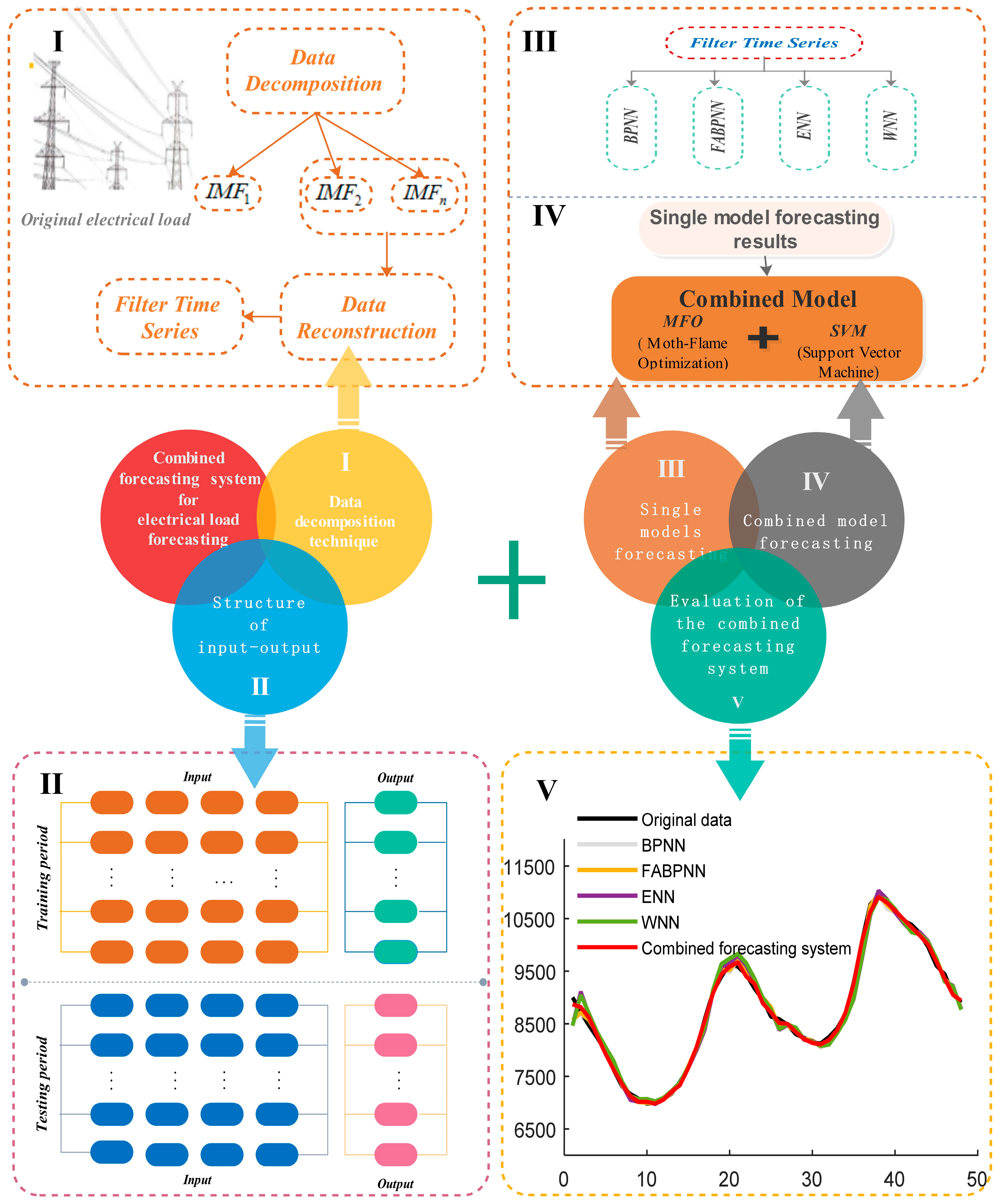
2. Framework of Proposed Nonlinear Combined Forecasting System
- ◆
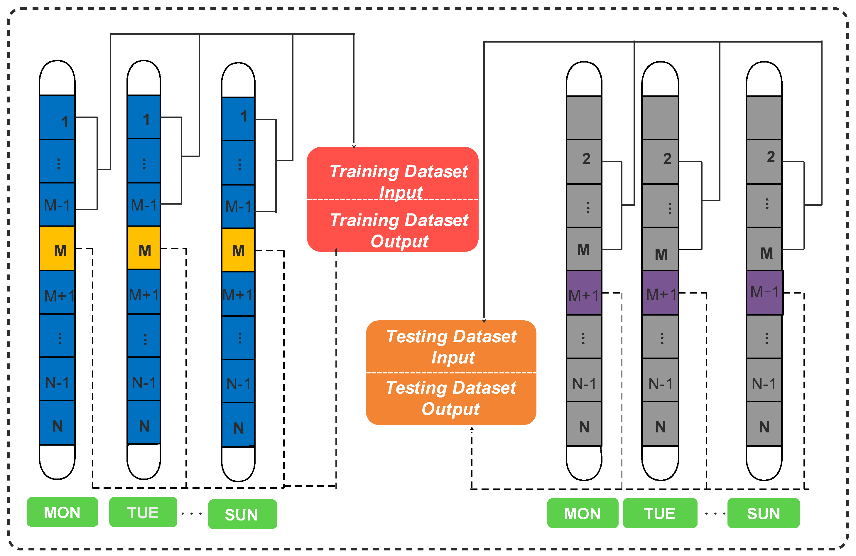
- Considering that uncertainty and randomness exist in raw electrical load series, the data pre-processing module improved by longitudinal data selection is employed during the first stage of electrical load forecasting to extract the primary features of the raw electrical load series.
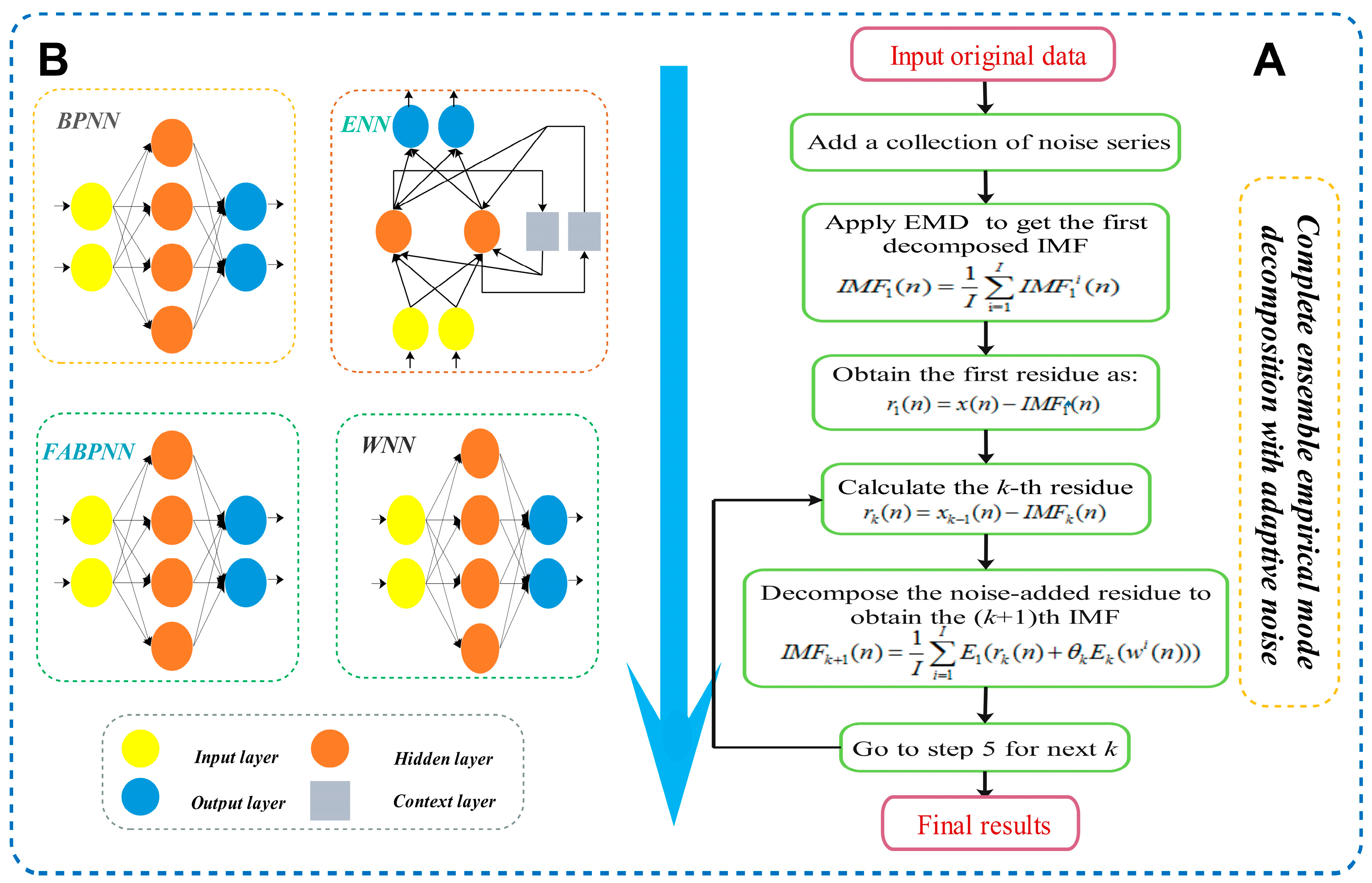
- ◆
- Four ANNs, namely BPNN, FABPNN, ENN and WNN, which are regarded as the individual forecasting models, are constructed to predict the filtered load time series. Then the combination forecasting is constructed based on modified SVM, which is used to combine the forecasting results obtained by the BPNN, FABPNN, ENN and WNN.
- ◆
- The prediction performance of the developed forecasting system is evaluated by employing typical accurate metrics, the Diebold–Mariano (DM) test and forecasting effectiveness.
- ◆
- Multi-step forecasting is applied in order to further test the forecasting abilities of the proposed combined forecasting system. Multi-step forecasting is an extrapolation process for realizing forecasting values by means of historical data and previous forecasting values. The multi-step forecasting process is as follows:
- (a)
- 1-step forecasting: on the basis of the historical data , the predicted data is acquired, where M is the sampled time of the data sequence.
- (b)
- 2-step forecasting: on the basis of the historical data and previously predicted value , the predicted data is acquired.
- (c)
- 3-step forecasting: on the basis of the historical data and previously predicted value , the predicted data is acquired.
3. Proposed Combined Forecasting System
3.1. Module 1: Improved Data Pre-Processing Module
3.2. Module 2: Forecasting Module
3.2.1. Individual Forecasting Models
3.2.2. Combined Forecasting Model
The Theory of Combined Forecasting
Support Vector Machine (SVM)
Moth-Flame Optimization (MFO)
| Algorithm 1 Moth-Flame Optimization Algorithm. | ||||
 | ||||
Construction of the Final Forecasting Result
3.3. Module 3: Evaluation
3.3.1. Forecasting System Evaluation Criteria
3.3.2. DM Test
3.3.3. Forecasting Effectiveness
4. Experimental Study
4.1. Data Selection
4.2. Experiment Setup
4.2.1. Experiment I: The Case of February
- (a)
- Table 4 shows the prediction capability of the combined forecasting system and four single models in the 1-step to 3-step forecasting. Taking Fridays’ forecasting results as an example: in 1-step forecasting, it is determined that the proposed nonlinear combined forecasting system achieves superior results compared to other models for different forecasting horizons. The combined forecasting system exhibits minimum forecasting errors, with AE, MAE, MSE, and MAPE values of −3.7850, 41.5131, 2979.40, and 0.4739%, respectively. The forecasting ability of BPNN is ranked second, while WNN exhibits the worst forecasting performance. In 2-step forecasting, the combined forecasting system achieves the most exact prediction performance, with a MAPE value of 0.8163%, while BPNN is the second most accurate model, and WNN is the worst. For 3-step forecasting, the combined forecasting system still achieves the most superior performance. The 1-step forecasting exhibits superior forecasting accuracy for the same model compared with multi-step prediction.
- (b)
- Table 5 presents the detailed results of multi-step improvements between the developed combined forecasting system and other prediction models. Taking Fridays’ results: in the 1-step predictions, the combined forecasting system decreases the MAE values by 57.4973%, 58.9966%, 61.2416% and 71.2267%, the MSE values by 82.4779%, 83.4804%, 84.4607% and 91.0522%, and the MAPE values by 57.6094%, 59.3157%, 61.7676% and 72.2005%, based on BPNN, FABPNN, ENN and WNN, respectively. In the 2-step and 3-step predictions, the combined forecasting system still decreases the MAE, MSE and MAPE values in comparison with other models.
- (c)
- Table 6 shows the statistical values of MAPE (%). The developed combined forecasting system obtains lower minimum and maximum MAPE values among the four individual models for 1-step to 3-step prediction. Furthermore, the developed forecasting system achieves minimum standard deviation (Std.) values for MAPE compared to the individual models.
- (d)
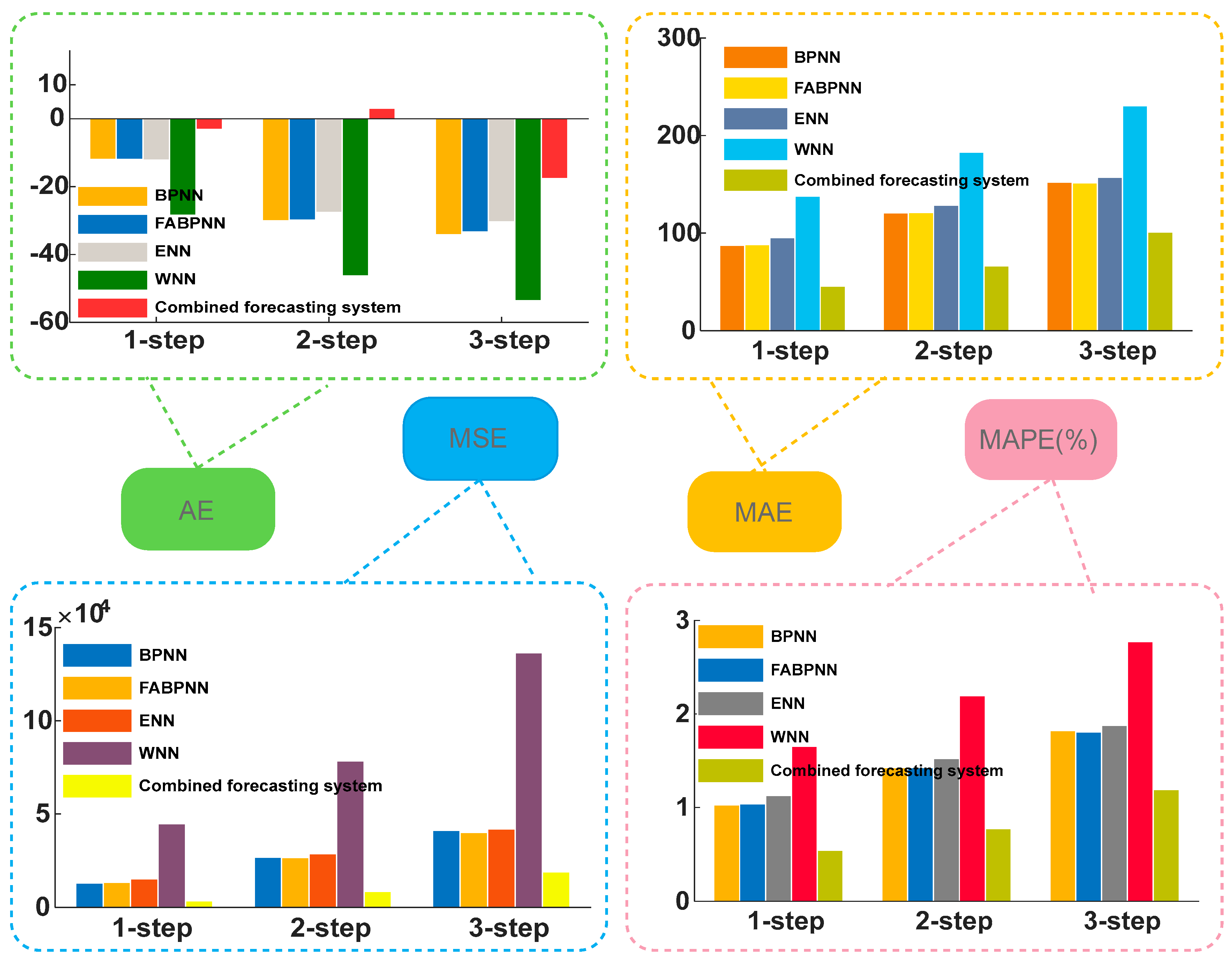
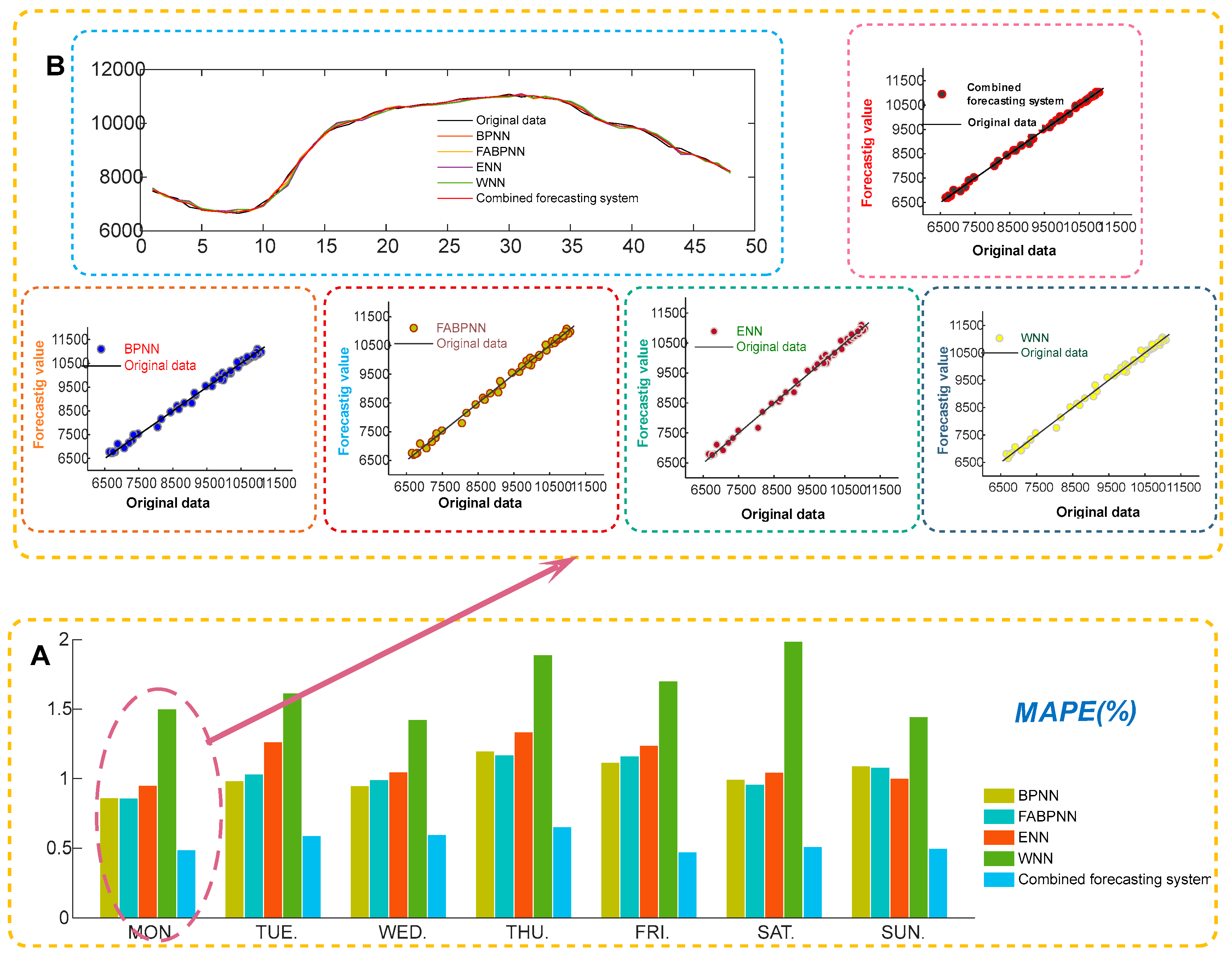
- Figure 4 displays the average values of AE, MAE, MSE and MAPE for 1-step, 2-step, and 3-step forecasting. To analyze the detailed forecasting results, the 1-step forecasting results for Monday are depicted in Figure 5. It can be observed that the prediction validity of the proposed nonlinear combined forecasting system is more precise than that of the single models. Moreover, the forecasting values of the developed forecasting system are more approximate to the real data.
4.2.2. Experiment II: The Case of June
- (a)
- Table 7 shows the final evaluations of the results for the 1-step to 3-step forecasting. For 1-step forecasting, the proposed combined forecasting system outperforms the BPNN, FABPNN, ENN and WNN models, according to the comparison of AE, MAE, MSE and MAPE from Monday to Sunday. For example, the MAPE values of the combined forecasting system are 0.5270%, 0.5390%, 0.4489%, 0.5306%, 0.4429%, 0.5052% and 0.5332% from Monday to Sunday, respectively. For 2-step forecasting, the developed combined forecasting system achieves the most accurate prediction effect, with MAPE values of 0.8562%, 0.7543%, 0.7336%, 0.8335%, 0.6223%, 0.6898% and 0.7702% from Monday to Sunday, respectively. For 3-step forecasting, the developed nonlinear combined forecasting system is still the most accurate.
- (b)
- Table 8 illustrates the detailed multi-step improvements between the developed combined forecasting system and other prediction models. Taking the results of Sunday as an example, in the 1-step predictions, the combined forecasting system decreases the MAPE values by 49.1983%, 47.7906%, 59.3493% and 65.0099%, based on BPNN, FABPNN, ENN and WNN, respectively. In the 2-step and 3-step predictions, the proposed combined forecasting system also decreases the MAPE values.
- (c)
- Table 9 displays the results of the MAPE value statistics. For the minimum, maximum, mean and Std. of the MAPE values, the developed combined forecasting system obtains a lower value in all aspects for BPNN, FABPNN, ENN and WNN.
- (d)
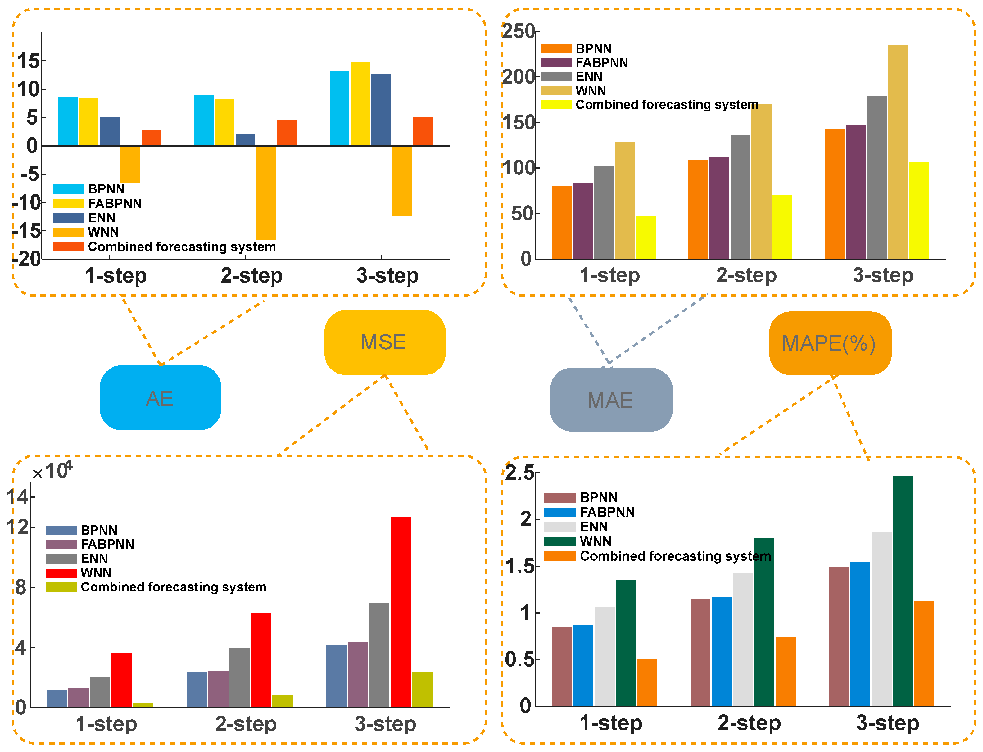
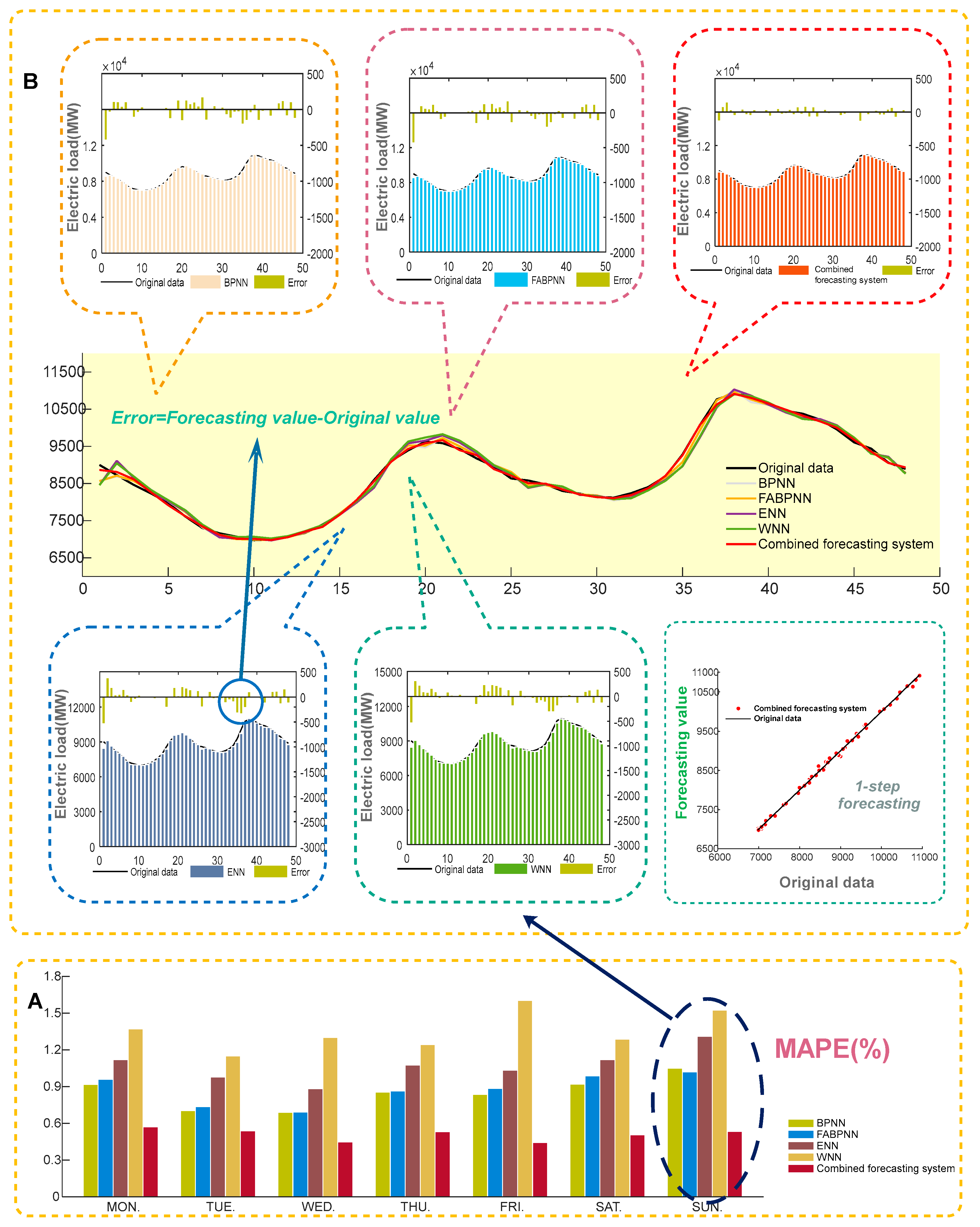
- Figure 6 summarizes the results of the average values of four forecasting error indexes for 1-step, 2-step, and 3-step forecasting in June. Furthermore, Figure 7 illustrates the detailed forecasting results of 1-step for Sunday. It is found that the combined forecasting system achieves a more precise prediction performance than the other four models.
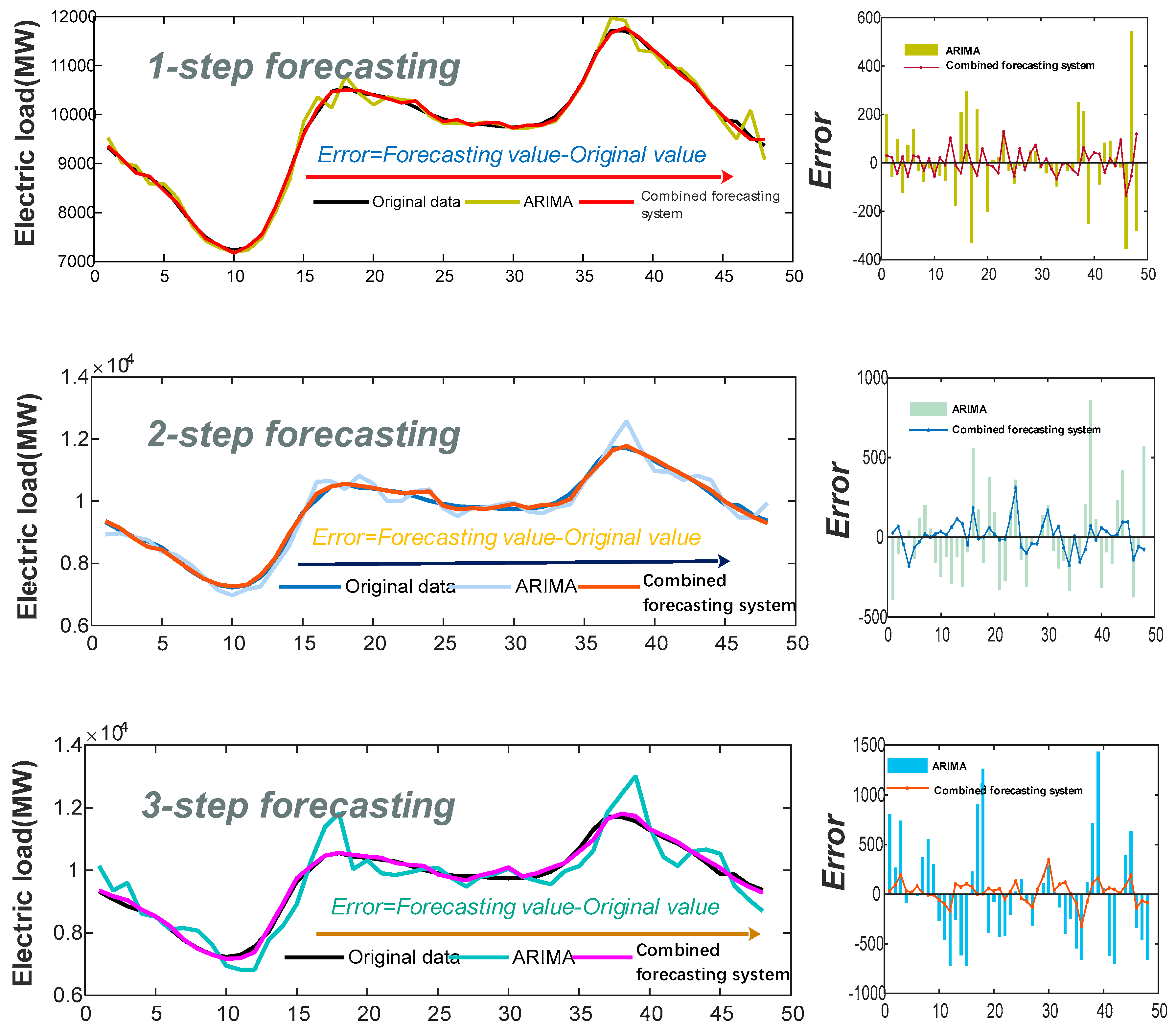
4.2.3. Experiment III: Comparison with Benchmark Model
4.3. Summary
- (a)
- For 1-step to 3-step forecasting, the developed combined forecasting system achieves smaller values for all forecasting error metrics than the single models. In addition, the developed combined forecasting system also obtains the lowest MAPE Std. results. Overall, through improved data preprocessing method and modified SVM, the developed system is superior to the four single models in terms of both validity and stability.
- (b)
- The developed combined forecasting system achieves lower MAPE results than the benchmark ARIMA model in 1-step to 3-step forecasting. Therefore, we can conclude that the developed combined forecasting system outperforms the ARIMA model in electrical load forecasting.
- (c)
- Compared with the individual prediction models, the predictive ability of the developed combined forecasting system exhibits significant improvements. According to relevant literature [3], if the electrical load forecasting error were to decrease by 1%, the operating costs would decrease by 10 million pounds. Consequently, considerable economic benefit could be generated.
5. Discussion
5.1. Discussion of the Significance of the Developed Forecasting System with Testing Method
- (a)
- Table 11 presents the DM statistics, where the square error loss function values are applied, and demonstrates that the combined forecasting system differs from BPNN, FABPNN, ENN, WNN and ARIMA at the 1% significance level in multi-step forecasting.
- (b)
- Table 11 implies the one-order and two-order forecasting effectiveness of the developed forecasting system and other compared models. From Table 11, it can be determined that the proposed forecasting system obtains the largest value of forecasting effectiveness compared with other compared models in multi-step forecasting.
5.2. Discussion of Comparison with Linear Combined Models
5.3. Discussion of the Superiority of the Optimization Algorithm
5.4. Further Validation for the Stability of the Developed Combined Forecasting System
6. Conclusions
Acknowledgments
Author Contributions
Conflicts of Interest
References
- Quan, H.; Srinivasan, D.; Khosravi, A. Uncertainty handling using neural network-based prediction intervals for electrical load forecasting. Energy 2014, 73, 916–925. [Google Scholar] [CrossRef]
- Shu, F.; Luonan, C. Short-term load forecasting based on an adaptive hybrid method. Power Syst. IEEE Trans. 2006, 21, 392–401. [Google Scholar] [CrossRef]
- Lee, C.-W.; Lin, B.-Y. Application of Hybrid Quantum Tabu Search with Support Vector Regression (SVR) for Load Forecasting. Energies 2016, 9, 873. [Google Scholar] [CrossRef]
- Zjavka, L.; Snášel, V. Short-term power load forecasting with ordinary differential equation substitutions of polynomial networks. Electr. Power Syst. Res. 2016, 137, 113–123. [Google Scholar] [CrossRef]
- Du, P.; Wang, J.; Yang, W.; Niu, T. Multi-step ahead forecasting in electrical power system using a hybrid forecasting system. Renew. Energy 2018, 122, 533–550. [Google Scholar] [CrossRef]
- Yang, W.; Wang, J.; Wang, R. Research and application of a novel hybrid model based on data selection and artificial intelligence algorithm for short term load forecasting. Entropy 2017, 19, 52. [Google Scholar] [CrossRef]
- The 12 Biggest Blackouts in History. Available online: http://www.msn.com/en-za/news/offbeat/the-12-biggest-blackouts-in-history/ar-CCeNdC#page=1 (accessed on 13 March 2018).
- Wang, Y.; Wang, J.; Zhao, G.; Dong, Y. Application of residual modification approach in seasonal ARIMA for electricity demand forecasting: A case study of China. Energy Policy 2012, 48, 284–294. [Google Scholar] [CrossRef]
- Huang, M.-L. Hybridization of Chaotic Quantum Particle Swarm Optimization with SVR in Electric Demand Forecasting. Energies 2016, 9, 426. [Google Scholar] [CrossRef]
- Dudek, G. Pattern-based local linear regression models for short-term load forecasting. Electr. Power Syst. Res. 2016, 130, 139–147. [Google Scholar] [CrossRef]
- Guo, Y.; Nazarian, E.; Ko, J.; Rajurkar, K. Hourly cooling load forecasting using time-indexed ARX models with two-stage weighted least squares regression. Energy Convers. Manag. 2014, 80, 46–53. [Google Scholar] [CrossRef]
- Wang, X. Grey prediction with rolling mechanism for electricity demand forecasting of Shanghai. In Proceedings of the 2007 IEEE International Conference on Grey Systems and Intelligent Services, GSIS 2007, Nanjing, China, 18–20 November 2007; pp. 689–692. [Google Scholar]
- Dong, Y.; Wang, J.; Wang, C.; Guo, Z. Research and Application of Hybrid Forecasting Model Based on an Optimal Feature Selection System—A Case Study on Electrical Load Forecasting. Energies 2017, 10, 490. [Google Scholar] [CrossRef]
- Lee, C.M.; Ko, C.N. Short-term load forecasting using lifting scheme and ARIMA models. Expert Syst. Appl. 2011, 38, 5902–5911. [Google Scholar] [CrossRef]
- Zhang, M.; Bao, H.; Yan, L.; Cao, J.; Du, J. Research on processing of short-term historical data of daily load based on Kalman filter. Power Syst Technol. 2003, 9, 39–42. [Google Scholar]
- Lin, W.-M.; Gow, H.-J.; Tsai, M.-T. An enhanced radial basis function network for short-term electricity price forecasting. Appl. Energy 2010, 87, 3226–3234. [Google Scholar] [CrossRef]
- Jain, R.K.; Smith, K.M.; Culligan, P.J.; Taylor, J.E. Forecasting energy consumption of multi-family residential buildings using support vector regression: Investigating the impact of temporal and spatial monitoring granularity on performance accuracy. Appl. Energy 2014, 123, 168–178. [Google Scholar] [CrossRef]
- García-Martos, C.; Rodríguez, J.; Sánchez, M.J. Modelling and forecasting fossil fuels, CO2 and electricity prices and their volatilities. Appl. Energy 2013, 101, 363–375. [Google Scholar] [CrossRef]
- Metaxiotis, K.; Kagiannas, A.; Askounis, D.; Psarras, J. Artificial intelligence in short term electric load forecasting: A state-of-the-art survey for the researcher. Energy Convers. Manag. 2003, 44, 1525–1534. [Google Scholar] [CrossRef]
- Li, P.; Li, Y.; Xiong, Q.; Chai, Y.; Zhang, Y. Application of a hybrid quantized Elman neural network in short-term load forecasting. Int. J. Electr. Power Energy Syst. 2014, 55, 749–759. [Google Scholar] [CrossRef]
- Liao, G.-C.; Tsao, T.-P. Application of fuzzy neural networks and artificial intelligence for load forecasting. Electr. Power Syst. Res. 2004, 70, 237–244. [Google Scholar] [CrossRef]
- Dong, Y.; Ma, X.; Ma, C.; Wang, J. Research and application of a hybrid forecasting model based on data decomposition for electrical load forecasting. Energies 2016, 9, 50. [Google Scholar] [CrossRef]
- Wang, J.; Yang, W.; Du, P.; Li, Y. Research and application of a hybrid forecasting framework based on multi-objective optimization for electrical power system. Energy 2018, 148, 59–78. [Google Scholar] [CrossRef]
- Li, H.; Guo, S.; Zhao, H.; Su, C.; Wang, B. Annual electric load forecasting by a least squares support vector machine with a fruit fly optimization algorithm. Energies 2012, 5, 4430–4445. [Google Scholar] [CrossRef]
- Peng, L.L.; Fan, G.F.; Huang, M.L.; Hong, W.C. Hybridizing DEMD and quantum PSO with SVR in electric load forecasting. Energies 2016, 9, 221. [Google Scholar] [CrossRef]
- Wang, J.; Yang, W.; Du, P.; Niu, T. A novel hybrid forecasting system of wind speed based on a newly developed multi-objective sine cosine algorithm. Energy Convers. Manag. 2018, 163, 134–150. [Google Scholar] [CrossRef]
- Wang, J.; Zhu, W.; Zhang, W.; Sun, D. A trend fixed on firstly and seasonal adjustment model combined with the ε-SVR for short-term forecasting of electricity demand. Energy Policy 2009, 37, 4901–4909. [Google Scholar] [CrossRef]
- Osório, G.J.; Matias, J.C.O.; Catalão, J.P.S. Short-term wind power forecasting using adaptive neuro-fuzzy inference system combined with evolutionary particle swarm optimization, wavelet transform and mutual information. Renew. Energy 2015, 75, 301–307. [Google Scholar] [CrossRef]
- Bates, J.M.; Granger, C.W.J. The Combination of Forecasts. Oper. Res. Soc. 1969, 20, 451–468. [Google Scholar] [CrossRef]
- Wang, J.; Zhu, S.; Zhang, W.; Lu, H. Combined modeling for electric load forecasting with adaptive particle swarm optimization. Energy 2010, 35, 1671–1678. [Google Scholar] [CrossRef]
- Xiao, L.; Wang, J.; Hou, R.; Wu, J. A combined model based on data pre-analysis and weight coefficients optimization for electrical load forecasting. Energy 2015, 82, 524–549. [Google Scholar] [CrossRef]
- Zhao, W.; Wang, J.; Lu, H. Combining forecasts of electricity consumption in China with time-varying weights updated by a high-order Markov chain model. Omega 2014, 45, 80–91. [Google Scholar] [CrossRef]
- Xiao, L.; Shao, W.; Liang, T.; Wang, C. A combined model based on multiple seasonal patterns and modified firefly algorithm for electrical load forecasting. Appl. Energy 2016, 167, 135–153. [Google Scholar] [CrossRef]
- Li, M.W.; Han, D.F.; Wang, W. long Vessel traffic flow forecasting by RSVR with chaotic cloud simulated annealing genetic algorithm and KPCA. Neurocomputing 2015, 157, 243–255. [Google Scholar] [CrossRef]
- Xu, Y.; Yang, W.; Wang, J. Air quality early-warning system for cities in China. Atmos. Environ. 2017, 148, 239–257. [Google Scholar] [CrossRef]
- Hong, W.C.; Dong, Y.; Zhang, W.Y.; Chen, L.Y.; Panigrahi, B.K. Cyclic electric load forecasting by seasonal SVR with chaotic genetic algorithm. Int. J. Electr. Power Energy Syst. 2013, 44, 604–614. [Google Scholar] [CrossRef]
- Chen, Y.; Hong, W.-C.; Shen, W.; Huang, N. Electric Load Forecasting Based on a Least Squares Support Vector Machine with Fuzzy Time Series and Global Harmony Search Algorithm. Energies 2016, 9, 70. [Google Scholar] [CrossRef]
- Hong, W.C.; Dong, Y.; Lai, C.Y.; Chen, L.Y.; Wei, S.Y. SVR with hybrid chaotic immune algorithm for seasonal load demand forecasting. Energies 2011, 4, 960–977. [Google Scholar] [CrossRef]
- Huang, N.; Shen, Z.; Long, S.; Wu, M.; Shih, H.; Zheng, Q.; Yen, N.; Tung, C.; Liu, H. The empirical mode decomposition and the Hilbert spectrum for nonlinear and non-stationary time series analysis. Proc. R. Soc. A Math. Phys. Eng. Sci. 1998, 454, 903–995. [Google Scholar] [CrossRef]
- Fan, G.F.; Peng, L.L.; Zhao, X.; Hong, W.C. Applications of hybrid EMD with PSO and GA for an SVR-based load forecasting model. Energies 2017, 10, 1713. [Google Scholar] [CrossRef]
- Fan, G.F.; Peng, L.L.; Hong, W.C.; Sun, F. Electric load forecasting by the SVR model with differential empirical mode decomposition and auto regression. Neurocomputing 2016, 173, 958–970. [Google Scholar] [CrossRef]
- Fan, G.-F.; Qing, S.; Wang, H.; Hong, W.-C.; Li, H.-J. Support vector regression model based on empirical mode decomposition and auto regression for electric load forecasting. Energies 2013, 6, 1887–1901. [Google Scholar] [CrossRef]
- Wu, Z.; Huang, N.E. Ensemble Empirical Mode Decomposition. Adv. Adapt. Data Anal. 2009, 1, 1–41. [Google Scholar] [CrossRef]
- Torres, M.E.; Colominas, M.A.; Schlotthauer, G.; Flandrin, P. A complete ensemble empirical mode decomposition with adaptive noise. In Proceedings of the IEEE International Conference on Acoustics, Speech and Signal Processing (ICASSP), Prague, Czech Republic, 22–26 May 2011; pp. 4144–4147. [Google Scholar]
- Zhang, W.; Qu, Z.; Zhang, K.; Mao, W.; Ma, Y.; Fan, X. A combined model based on CEEMDAN and modified flower pollination algorithm for wind speed forecasting. Energy Convers. Manag. 2017, 136, 439–451. [Google Scholar] [CrossRef]
- Afanasyev, D.O.; Fedorova, E.A. The long-term trends on the electricity markets: Comparison of empirical mode and wavelet decompositions. Energy Econ. 2016, 56, 432–442. [Google Scholar] [CrossRef]
- Chen, Y.; Yang, Y.; Liu, C.; Li, C.; Li, L. A hybrid application algorithm based on the support vector machine and artificial intelligence: An example of electric load forecasting. Appl. Math. Model. 2015, 39, 2617–2632. [Google Scholar] [CrossRef]
- Vapnik, V.N. The Nature of Statistical Learning Theory; Springer: New York, NY, USA, 1995. [Google Scholar]
- Vapnik, V.N. Statistical Learning Theory; Wiley: New York, NY, USA, 1998. [Google Scholar]
- Ju, F.Y.; Hong, W.C. Application of seasonal SVR with chaotic gravitational search algorithm in electricity forecasting. Appl. Math. Model. 2013, 37, 9643–9651. [Google Scholar] [CrossRef]
- Li, M.W.; Geng, J.; Wang, S.; Hong, W.C. Hybrid chaotic quantum bat algorithm with SVR in electric load forecasting. Energies 2017, 10, 2180. [Google Scholar] [CrossRef]
- Liang, Y.; Niu, D.; Ye, M.; Hong, W.-C. Short-term load forecasting based on wavelet transform and least squares support vector machine optimized by improved cuckoo search. Energies 2016, 9, 827. [Google Scholar] [CrossRef]
- Mirjalili, S. Moth-flame optimization algorithm: A novel nature-inspired heuristic paradigm. Knowl.-Based Syst. 2015, 89, 228–249. [Google Scholar] [CrossRef]
- Zhao, H.; Zhao, H.; Guo, S. Using GM (1,1) Optimized by MFO with Rolling Mechanism to Forecast the Electricity Consumption of Inner Mongolia. Appl. Sci. 2016, 6, 20. [Google Scholar] [CrossRef]
- Diebold, F.X.; Mariano, R.S. Comparing predictive accuracy. J. Bus. Econ. Stat. 1995, 13, 253–263. [Google Scholar] [CrossRef]
- Chen, H.; Hou, D. Research on superior combination forecasting model based on forecasting effective measure. J. Univ. Sci. Technol. China 2002, 2, 172–180. [Google Scholar]
- Wang, J.; Du, P.; Niu, T.; Yang, W. A novel hybrid system based on a new proposed algorithm—Multi-objective Whale Optimization Algorithm for wind speed forecasting. Appl. Energy 2017, 208, 344–360. [Google Scholar] [CrossRef]


| Metric | Definition | Equation |
|---|---|---|
| AE | The average error of T forecasting results | |
| MAE | The mean error absolute of T forecasting results | |
| MSE | The mean square error of T forecasting results | |
| MAPE (%) | The mean absolute percentage error | |
| 1 (%) | The decreased relative error of the index among different models |
| Model | Experimental Parameter | Default Value |
|---|---|---|
| CEEMDAN | Noise standard deviation | 0.2 |
| The number of realizations | 500 | |
| Maximum number of sifting iterations | 5000 | |
| The removed intrinsic mode functions | IMF1 | |
| BPNN | Learning velocity | 0.1 |
| Maximum number of training iterations | 1000 | |
| Training precision requirement | 0.00004 | |
| Neuron number in the input layer | 4 | |
| Neuron number in the hidden layer | 9 | |
| Neuron number in the output layer | 1 | |
| FABPNN | FA number of fireflies | 30 |
| Maximum number of FA iterations | 500 | |
| FA randomness 0–1 | 0.5 | |
| FA minimum value of beta | 0.2 | |
| FA absorption coefficient | 1 | |
| BPNN maximum number of iteration times | 200 | |
| BPNN convergence value | 0.00001 | |
| BPNN learning rate | 0.1 | |
| Neuron number in the input layer | 4 | |
| Neuron number in the hidden layer | 9 | |
| Neuron number in the output layer | 1 | |
| ENN | Number of iterations | 1000 |
| Neuron number in the input layer | 4 | |
| Neuron number in the hidden layer | 9 | |
| Neuron number in the output layer | 1 | |
| WNN | Number of iterations | 100 |
| Learning rate | 0.01 | |
| Neuron number in the input layer | 4 | |
| Neuron number in the hidden layer | 9 | |
| Neuron number in the output layer | 1 | |
| MFO | The number of search agents | 30 |
| Maximum number of iterations | 300 | |
| The lower bounds of variables | 0.01 | |
| The upper bounds of variables | 100 | |
| The number of variables | 2 | |
| SVM | The number of the input layer | 4 |
| The number of the output layer | 1 | |
| The kernel function’s name | RBF |
| Week | Month | Mean | Median | Std. | Minimum | Maximum |
|---|---|---|---|---|---|---|
| (MW) | (MW) | (MW) | (MW) | (MW) | ||
| MON. | February | 9334.305 | 9871.095 | 1520.628 | 6649.840 | 11,078.940 |
| June | 9720.624 | 9952.190 | 1409.115 | 7157.530 | 11,937.500 | |
| TUE. | February | 8589.615 | 9019.185 | 1073.913 | 6488.980 | 9683.760 |
| June | 9920.198 | 10,129.775 | 1238.084 | 7453.350 | 11,996.360 | |
| WED. | February | 8649.826 | 9031.205 | 1111.026 | 6452.950 | 9786.950 |
| June | 9682.923 | 9848.785 | 1189.045 | 7228.830 | 11,713.400 | |
| THU. | February | 8864.992 | 9374.700 | 1255.005 | 6487.110 | 10,273.970 |
| June | 9603.785 | 9743.965 | 1206.705 | 7140.740 | 11,602.130 | |
| FRI. | February | 8870.044 | 9170.695 | 1237.710 | 6516.410 | 10,200.400 |
| June | 9735.629 | 9894.510 | 1182.482 | 7327.950 | 11,451.680 | |
| SAT. | February | 8540.942 | 8979.640 | 1133.162 | 6554.520 | 9928.520 |
| June | 9124.386 | 9226.755 | 982.705 | 7268.430 | 10,864.100 | |
| SUN. | February | 8093.038 | 8554.020 | 1001.747 | 6391.530 | 9390.940 |
| June | 8772.331 | 8663.305 | 1116.673 | 6977.150 | 10,926.030 |
| Week | Model | AE | MAE | MSE | MAPE | ||||||||
|---|---|---|---|---|---|---|---|---|---|---|---|---|---|
| 1-Step | 2-Step | 3-Step | 1-Step | 2-Step | 3-Step | 1-Step | 2-Step | 3-Step | 1-Step | 2-Step | 3-Step | ||
| MON. | BPNN | 1.3639 | −10.7514 | −14.7858 | 76.9680 | 87.3096 | 126.8697 | 9493.46 | 12,421.47 | 27,525.35 | 0.8632 | 0.9558 | 1.4429 |
| FABPNN | 3.7445 | −6.6519 | −5.2474 | 76.7589 | 88.2479 | 128.2259 | 9547.03 | 12,511.88 | 28,258.78 | 0.8612 | 0.9670 | 1.4564 | |
| ENN | −1.0044 | −13.5185 | −15.2619 | 84.9175 | 105.2535 | 152.5501 | 12,425.12 | 18,729.96 | 41,127.41 | 0.9535 | 1.1599 | 1.7416 | |
| WNN | −0.1408 | −25.7658 | −26.4372 | 134.9493 | 174.9007 | 236.5244 | 32,121.24 | 66,146.46 | 183,341.01 | 1.5029 | 1.9178 | 2.6471 | |
| Combined forecasting system | −1.8954 | 4.8475 | −25.3053 | 42.7547 | 55.7483 | 92.0454 | 2955.29 | 5066.13 | 15,392.98 | 0.4896 | 0.6125 | 1.0435 | |
| TUE. | BPNN | −14.0677 | −23.9245 | −32.1850 | 82.8839 | 104.7622 | 135.1333 | 11,424.72 | 19,811.92 | 32,025.02 | 0.9856 | 1.2580 | 1.6543 |
| FABPNN | −16.8212 | −28.3703 | −39.8426 | 87.0675 | 111.3953 | 140.6762 | 12,832.80 | 22,262.70 | 34,626.02 | 1.0341 | 1.3385 | 1.7184 | |
| ENN | −20.6985 | −32.9486 | −42.9214 | 104.1221 | 134.5153 | 158.6410 | 17,145.19 | 30,481.01 | 45,606.38 | 1.2659 | 1.6504 | 1.9700 | |
| WNN | −18.6602 | −31.9576 | −50.3965 | 132.1093 | 179.5787 | 231.9993 | 32,314.95 | 95,482.40 | 228,634.12 | 1.6168 | 2.2088 | 2.8686 | |
| Combined forecasting system | −3.5775 | −3.1009 | −1.3271 | 48.7534 | 72.6386 | 109.7521 | 3697.70 | 9420.42 | 21,857.92 | 0.5921 | 0.8679 | 1.3137 | |
| WED. | BPNN | −17.0143 | −31.5453 | −35.0435 | 79.8144 | 113.2511 | 144.3384 | 10,635.37 | 23,724.32 | 36,327.29 | 0.9491 | 1.3497 | 1.7504 |
| FABPNN | −15.8284 | −30.8274 | −33.7778 | 83.1057 | 113.8130 | 139.9802 | 11,747.10 | 24,310.67 | 34,389.39 | 0.9930 | 1.3608 | 1.6969 | |
| ENN | −13.7888 | −25.2383 | −26.1058 | 87.7993 | 117.0281 | 142.4337 | 13,134.19 | 25,093.04 | 35,466.31 | 1.0498 | 1.3961 | 1.7187 | |
| WNN | −11.8223 | −12.5006 | −3.6612 | 118.3172 | 160.6506 | 198.1202 | 41,894.21 | 58,325.44 | 79,324.94 | 1.4270 | 1.9408 | 2.3941 | |
| Combined forecasting system | −8.1485 | −9.1175 | −28.6959 | 49.4339 | 68.0790 | 104.9988 | 4082.45 | 9029.29 | 21,231.04 | 0.5998 | 0.8124 | 1.2458 | |
| THU. | BPNN | −6.3561 | −19.6933 | −22.5452 | 104.6001 | 132.4169 | 174.4194 | 17,715.78 | 32,893.48 | 47,678.25 | 1.2009 | 1.5345 | 2.0338 |
| FABPNN | −8.0497 | −22.9996 | −23.4411 | 102.1040 | 129.9880 | 166.0143 | 17,458.21 | 32,981.15 | 43,922.02 | 1.1714 | 1.5080 | 1.9394 | |
| ENN | −14.2674 | −30.6256 | −29.6502 | 114.5853 | 143.5429 | 171.5193 | 21,097.11 | 36,114.88 | 45,852.66 | 1.3363 | 1.6930 | 2.0229 | |
| WNN | −33.6208 | −53.1476 | −63.9543 | 160.5429 | 200.8806 | 247.5782 | 45,415.21 | 82,931.44 | 124,086.68 | 1.8929 | 2.3803 | 2.9301 | |
| Combined forecasting system | −6.5061 | −10.1216 | −4.2527 | 55.5226 | 80.3931 | 123.8744 | 4824.10 | 12,375.84 | 24,987.70 | 0.6553 | 0.9407 | 1.4463 | |
| FRI. | BPNN | −10.2567 | −23.5966 | −21.2707 | 97.6717 | 140.9842 | 187.9748 | 17,003.61 | 37,922.83 | 61,624.94 | 1.1179 | 1.6060 | 2.1836 |
| FABPNN | −14.0009 | −28.2144 | −28.2492 | 101.2430 | 147.2809 | 198.5211 | 18,035.56 | 41,018.75 | 69,155.70 | 1.1647 | 1.6898 | 2.3062 | |
| ENN | −12.1384 | −27.6435 | −22.5750 | 107.1073 | 146.7995 | 190.7033 | 19,173.26 | 38,936.81 | 59,817.36 | 1.2394 | 1.7010 | 2.2384 | |
| WNN | −28.1042 | −47.9970 | −52.1578 | 144.2766 | 196.5340 | 258.1345 | 33,297.40 | 66,162.33 | 108,392.63 | 1.7046 | 2.3169 | 3.0409 | |
| Combined forecasting system | −3.7850 | −0.8954 | −3.4699 | 41.5131 | 71.7784 | 105.1659 | 2979.40 | 10,037.04 | 22,513.69 | 0.4739 | 0.8163 | 1.1747 | |
| SAT. | BPNN | −18.3668 | −58.8065 | −50.1905 | 83.6567 | 128.2100 | 149.5539 | 13,347.26 | 30,695.80 | 42,244.56 | 0.9949 | 1.5385 | 1.8127 |
| FABPNN | −18.2990 | −58.7480 | −52.0260 | 81.0710 | 122.2612 | 142.6670 | 12,678.25 | 27,997.98 | 37,079.79 | 0.9596 | 1.4585 | 1.7135 | |
| ENN | −8.9057 | −33.5612 | −33.2007 | 88.3301 | 129.8825 | 159.4560 | 13,860.60 | 28,814.81 | 43,314.43 | 1.0473 | 1.5408 | 1.8951 | |
| WNN | −76.2241 | −103.5840 | −110.5893 | 161.0754 | 203.1411 | 247.7138 | 107,836.75 | 137,768.64 | 166,982.05 | 1.9893 | 2.5032 | 3.0492 | |
| Combined forecasting system | −9.9972 | −15.8985 | −16.9380 | 42.2213 | 60.0048 | 97.4307 | 3253.00 | 7601.39 | 16,427.04 | 0.5115 | 0.7260 | 1.1988 | |
| SUN. | BPNN | −19.0006 | −41.8885 | −63.0577 | 87.1693 | 138.3510 | 146.6729 | 11,695.38 | 30,279.09 | 41,649.76 | 1.0927 | 1.7384 | 1.8840 |
| FABPNN | −14.7801 | −33.2463 | −50.9624 | 87.4692 | 134.0810 | 144.3636 | 11,198.22 | 26,233.76 | 34,582.41 | 1.0840 | 1.6733 | 1.8233 | |
| ENN | −14.2234 | −29.7956 | −42.5369 | 81.0386 | 123.0542 | 124.7987 | 10,251.81 | 22,741.01 | 23,536.69 | 1.0041 | 1.5374 | 1.5672 | |
| WNN | −30.0213 | −49.0184 | −68.3288 | 113.8393 | 164.9003 | 194.3404 | 19,452.64 | 42,417.10 | 64,463.36 | 1.4473 | 2.1072 | 2.5010 | |
| Combined forecasting system | −3.1120 | 3.1278 | −17.6043 | 40.6275 | 55.6796 | 74.5055 | 2549.95 | 5992.00 | 10,360.29 | 0.4988 | 0.6746 | 0.9197 | |
| Week | Combined Forecasting System | Combined Forecasting System | Combined Forecasting System | Combined Forecasting System | |||||||||
|---|---|---|---|---|---|---|---|---|---|---|---|---|---|
| vs. BPNN | vs. FABPNN | vs. ENN | vs. WNN | ||||||||||
| 1-Step | 2-Step | 3-Step | 1-Step | 2-Step | 3-Step | 1-Step | 2-Step | 3-Step | 1-Step | 2-Step | 3-Step | ||
| MON. | 44.4513 | 36.1488 | 27.4489 | 44.2999 | 36.8276 | 28.2162 | 49.6514 | 47.0343 | 39.6622 | 68.3179 | 68.1258 | 61.0842 | |
| 68.8703 | 59.2147 | 44.0771 | 69.0449 | 59.5094 | 45.5285 | 76.2152 | 72.9517 | 62.5725 | 90.7996 | 92.3410 | 91.6042 | ||
| 43.2778 | 35.9101 | 27.6819 | 43.1419 | 36.6539 | 28.3536 | 48.6478 | 47.1907 | 40.0867 | 67.4188 | 68.0597 | 60.5802 | ||
| TUE. | 41.1787 | 30.6634 | 18.7823 | 44.0051 | 34.7921 | 21.9825 | 53.1767 | 45.9998 | 30.8173 | 63.0962 | 59.5506 | 52.6929 | |
| 67.6343 | 52.4507 | 31.7474 | 71.1856 | 57.6852 | 36.8743 | 78.4330 | 69.0941 | 52.0727 | 88.5573 | 90.1339 | 90.4398 | ||
| 39.9223 | 31.0096 | 20.5897 | 42.7370 | 35.1567 | 23.5513 | 53.2227 | 47.4119 | 33.3134 | 63.3761 | 60.7058 | 54.2041 | ||
| 38.0639 | 39.8867 | 27.2551 | 40.5168 | 40.1834 | 24.9902 | 43.6966 | 41.8268 | 26.2823 | 58.2192 | 57.6229 | 47.0025 | ||
| WED. | 61.6144 | 61.9408 | 41.5562 | 65.2472 | 62.8587 | 38.2628 | 68.9174 | 64.0167 | 40.1375 | 90.2553 | 84.5191 | 73.2354 | |
| 36.7974 | 39.8068 | 28.8274 | 39.5934 | 40.2975 | 26.5832 | 42.8602 | 41.8081 | 27.5157 | 57.9655 | 58.1405 | 47.9638 | ||
| 46.9192 | 39.2879 | 28.9790 | 45.6216 | 38.1534 | 25.3833 | 51.5448 | 43.9937 | 27.7782 | 65.4157 | 59.9797 | 49.9655 | ||
| THU. | 72.7695 | 62.3760 | 47.5910 | 72.3678 | 62.4760 | 43.1089 | 77.1339 | 65.7320 | 45.5044 | 89.3778 | 85.0770 | 79.8627 | |
| 45.4345 | 38.6991 | 28.8866 | 44.0607 | 37.6218 | 25.4225 | 50.9610 | 44.4366 | 28.5023 | 65.3818 | 60.4796 | 50.6387 | ||
| FRI. | 57.4973 | 49.0877 | 44.0532 | 58.9966 | 51.2643 | 47.0253 | 61.2416 | 51.1045 | 44.8537 | 71.2267 | 63.4779 | 59.2593 | |
| 82.4779 | 73.5330 | 63.4666 | 83.4804 | 75.5306 | 67.4449 | 84.4607 | 74.2222 | 62.3626 | 91.0522 | 84.8297 | 79.2295 | ||
| 57.6094 | 49.1712 | 46.2056 | 59.3157 | 51.6906 | 49.0637 | 61.7676 | 52.0078 | 47.5228 | 72.2005 | 64.7666 | 61.3709 | ||
| SAT. | 49.5303 | 53.1980 | 34.8525 | 47.9206 | 50.9208 | 31.7076 | 52.2005 | 53.8007 | 38.8981 | 73.7879 | 70.4615 | 60.6680 | |
| 75.6279 | 75.2364 | 61.1144 | 74.3419 | 72.8502 | 55.6981 | 76.5306 | 73.6199 | 62.0749 | 96.9834 | 94.4825 | 90.1624 | ||
| 48.5887 | 52.8144 | 33.8674 | 46.6971 | 50.2268 | 30.0376 | 51.1612 | 52.8833 | 36.7424 | 74.2879 | 70.9991 | 60.6855 | ||
| SUN. | 53.3925 | 59.7548 | 49.2029 | 53.5523 | 58.4732 | 48.3903 | 49.8665 | 54.7520 | 40.2994 | 64.3116 | 66.2344 | 61.6624 | |
| 78.1970 | 80.2108 | 75.1252 | 77.2290 | 77.1592 | 70.0417 | 75.1268 | 73.6511 | 55.9824 | 86.8915 | 85.8736 | 83.9284 | ||
| 54.3518 | 61.1941 | 51.1820 | 53.9817 | 59.6848 | 49.5571 | 50.3214 | 56.1203 | 41.3132 | 65.5337 | 67.9861 | 63.2263 | ||
| Week | BPNN | FABPNN | ENN | WNN | Combined Forecasting System | |||||||||||
|---|---|---|---|---|---|---|---|---|---|---|---|---|---|---|---|---|
| 1-Step | 2-Step | 3-Step | 1-Step | 2-Step | 3-Step | 1-Step | 2-Step | 3-Step | 1-Step | 2-Step | 3-Step | 1-Step | 2-Step | 3-Step | ||
| MON. | Minimum | 0.8263 | 0.8868 | 1.2521 | 0.8120 | 0.8529 | 1.1331 | 0.8120 | 0.9274 | 1.2315 | 0.9705 | 1.1373 | 1.3787 | 0.4529 | 0.5472 | 0.8730 |
| Maximum | 0.9434 | 1.1193 | 1.7437 | 0.9823 | 1.2637 | 2.1828 | 1.0879 | 1.4398 | 2.1751 | 3.0041 | 4.0754 | 7.2584 | 0.5151 | 0.6505 | 1.2038 | |
| Mean | 0.8632 | 0.9558 | 1.4429 | 0.8612 | 0.9670 | 1.4564 | 0.9535 | 1.1599 | 1.7416 | 1.5029 | 1.9178 | 2.6471 | 0.4896 | 0.6125 | 1.0435 | |
| Std. | 0.0345 | 0.0657 | 0.1616 | 0.0487 | 0.1037 | 0.2740 | 0.0741 | 0.1385 | 0.2470 | 0.6015 | 0.9387 | 1.5568 | 0.0153 | 0.0289 | 0.0867 | |
| TUE. | Minimum | 0.8513 | 1.0494 | 1.3943 | 0.8942 | 1.1293 | 1.4114 | 0.9588 | 1.2102 | 1.4313 | 1.0894 | 1.3884 | 1.7998 | 0.5608 | 0.7945 | 1.0911 |
| Maximum | 1.1912 | 1.5185 | 1.9739 | 1.4806 | 1.8611 | 2.0036 | 1.5263 | 1.9735 | 2.3895 | 3.3843 | 6.9578 | 10.6987 | 0.6185 | 0.9187 | 1.5951 | |
| Mean | 0.9856 | 1.2580 | 1.6543 | 1.0341 | 1.3385 | 1.7184 | 1.2659 | 1.6504 | 1.9700 | 1.6168 | 2.2088 | 2.8686 | 0.5921 | 0.8679 | 1.3137 | |
| Std. | 0.0877 | 0.1299 | 0.1802 | 0.1493 | 0.2029 | 0.1622 | 0.1536 | 0.1937 | 0.2241 | 0.5693 | 1.3644 | 2.2010 | 0.0179 | 0.0366 | 0.1462 | |
| WED. | Minimum | 0.8988 | 1.1342 | 1.3668 | 0.8959 | 1.0632 | 1.2543 | 0.9589 | 1.1811 | 1.3829 | 1.0015 | 1.2242 | 1.4547 | 0.5303 | 0.7643 | 0.7724 |
| Maximum | 1.0376 | 1.4876 | 2.0036 | 1.3294 | 1.9717 | 2.3057 | 1.1692 | 1.5723 | 2.0403 | 3.2969 | 4.7078 | 4.4628 | 1.0370 | 0.8529 | 1.4643 | |
| Mean | 0.9491 | 1.3497 | 1.7504 | 0.9930 | 1.3608 | 1.6969 | 1.0498 | 1.3961 | 1.7187 | 1.4270 | 1.9408 | 2.3941 | 0.5998 | 0.8124 | 1.2458 | |
| Std. | 0.0376 | 0.0944 | 0.1750 | 0.1175 | 0.2126 | 0.2517 | 0.0692 | 0.1186 | 0.1846 | 0.5523 | 0.8268 | 0.6952 | 0.1223 | 0.0309 | 0.1919 | |
| THU. | Minimum | 1.1328 | 1.3555 | 1.7345 | 1.0592 | 1.2446 | 1.6240 | 1.1695 | 1.4815 | 1.7197 | 1.4439 | 1.6901 | 1.9451 | 0.5996 | 0.6861 | 1.2255 |
| Maximum | 1.6897 | 2.2229 | 3.1837 | 1.4571 | 2.0609 | 2.5822 | 1.4567 | 1.9075 | 2.4223 | 3.3581 | 5.0644 | 5.9695 | 0.6986 | 0.9970 | 1.7947 | |
| Mean | 1.2009 | 1.5345 | 2.0338 | 1.1714 | 1.5080 | 1.9394 | 1.3363 | 1.6930 | 2.0229 | 1.8929 | 2.3803 | 2.9301 | 0.6553 | 0.9407 | 1.4463 | |
| Std. | 0.1370 | 0.2010 | 0.3381 | 0.1043 | 0.1875 | 0.2672 | 0.0795 | 0.1300 | 0.2029 | 0.4819 | 0.8472 | 1.0381 | 0.0273 | 0.0761 | 0.1614 | |
| FRI. | Minimum | 0.9789 | 1.3521 | 1.8090 | 0.9879 | 1.3789 | 1.9802 | 1.1533 | 1.5778 | 2.0425 | 1.1984 | 1.6895 | 2.1985 | 0.4217 | 0.7267 | 0.9891 |
| Maximum | 1.3273 | 1.8529 | 2.6347 | 1.6243 | 2.1960 | 2.8817 | 1.5201 | 1.8915 | 2.4986 | 2.3440 | 3.0883 | 4.2423 | 0.5172 | 0.9259 | 1.4602 | |
| Mean | 1.1179 | 1.6060 | 2.1836 | 1.1647 | 1.6898 | 2.3062 | 1.2394 | 1.7010 | 2.2384 | 1.7046 | 2.3169 | 3.0409 | 0.4739 | 0.8163 | 1.1747 | |
| Std. | 0.0869 | 0.1481 | 0.2171 | 0.1625 | 0.2330 | 0.2601 | 0.0967 | 0.1050 | 0.1391 | 0.3505 | 0.4306 | 0.6477 | 0.0272 | 0.0508 | 0.1357 | |
| SAT. | Minimum | 0.8925 | 1.4090 | 1.5762 | 0.8792 | 1.3074 | 1.5122 | 0.9497 | 1.4249 | 1.6132 | 0.9158 | 1.1241 | 1.3579 | 0.4807 | 0.6395 | 1.0126 |
| Maximum | 1.0930 | 1.6887 | 2.1120 | 1.0835 | 1.6422 | 1.9560 | 1.2232 | 1.6595 | 2.1832 | 10.3437 | 11.1349 | 11.0434 | 0.5409 | 0.8148 | 1.4727 | |
| Mean | 0.9949 | 1.5385 | 1.8127 | 0.9596 | 1.4585 | 1.7135 | 1.0473 | 1.5408 | 1.8951 | 1.9893 | 2.5032 | 3.0492 | 0.5115 | 0.7260 | 1.1988 | |
| Std. | 0.0536 | 0.0912 | 0.1550 | 0.0573 | 0.0958 | 0.1237 | 0.0965 | 0.0795 | 0.1722 | 2.3444 | 2.4300 | 2.3140 | 0.0145 | 0.0472 | 0.1428 | |
| SUN. | Minimum | 0.9423 | 1.4501 | 1.4459 | 0.9174 | 1.3993 | 1.4387 | 0.9367 | 1.4470 | 1.4025 | 1.0703 | 1.6719 | 1.6650 | 0.4750 | 0.4991 | 0.7836 |
| Maximum | 1.7058 | 2.7597 | 3.6231 | 1.4369 | 1.9129 | 2.2679 | 1.1217 | 1.6749 | 1.8943 | 1.8294 | 2.6436 | 3.1335 | 0.5144 | 0.7494 | 1.0195 | |
| Mean | 1.0927 | 1.7384 | 1.8840 | 1.0840 | 1.6733 | 1.8233 | 1.0041 | 1.5374 | 1.5672 | 1.4473 | 2.1072 | 2.5010 | 0.4988 | 0.6746 | 0.9197 | |
| Std. | 0.2429 | 0.4149 | 0.6700 | 0.1215 | 0.1744 | 0.2622 | 0.0597 | 0.0552 | 0.1404 | 0.2072 | 0.2701 | 0.4509 | 0.0122 | 0.0784 | 0.0729 | |
| Week | Model | AE | MAE | MSE | MAPE | ||||||||
|---|---|---|---|---|---|---|---|---|---|---|---|---|---|
| 1-Step | 2-Step | 3-Step | 1-Step | 2-Step | 3-Step | 1-Step | 2-Step | 3-Step | 1-Step | 2-Step | 3-Step | ||
| MON. | BPNN | 28.1490 | 40.2809 | 60.0420 | 87.2188 | 116.6938 | 157.3218 | 12,598.62 | 24,248.91 | 46,240.92 | 0.9174 | 1.2500 | 1.6564 |
| FABPNN | 31.9426 | 43.4337 | 70.0051 | 91.8725 | 122.9630 | 174.0908 | 14,715.99 | 27,952.61 | 57,357.07 | 0.9592 | 1.3000 | 1.8176 | |
| ENN | 23.5497 | 25.6296 | 41.8058 | 107.7753 | 140.2308 | 191.1443 | 22,021.50 | 43,213.06 | 84,770.04 | 1.1190 | 1.4900 | 2.0180 | |
| WNN | 21.3635 | 24.2720 | 40.4258 | 131.7077 | 172.9343 | 259.7937 | 34,847.82 | 61,929.17 | 162,633.65 | 1.3722 | 1.8200 | 2.6891 | |
| Combined forecasting system | 13.1643 | 31.7783 | 33.2478 | 53.4406 | 81.4294 | 118.3925 | 4923.01 | 10,866.11 | 29,343.95 | 0.5720 | 0.8562 | 1.2510 | |
| TUE. | BPNN | 11.8632 | 11.0946 | 30.6152 | 68.8202 | 93.5565 | 118.4368 | 7209.00 | 14,736.01 | 27,030.99 | 0.7028 | 0.9400 | 1.1964 |
| FABPNN | 8.2711 | 4.7844 | 23.4885 | 72.6215 | 96.1279 | 127.4886 | 8652.02 | 16,947.82 | 31,041.00 | 0.7372 | 0.9600 | 1.2870 | |
| ENN | 9.9318 | 2.2467 | 25.5482 | 97.0374 | 117.4459 | 147.8419 | 16,480.67 | 30,382.58 | 52,207.81 | 0.9774 | 1.1800 | 1.4659 | |
| WNN | 8.3753 | 4.2323 | 24.5869 | 113.9295 | 142.2588 | 203.1351 | 22,966.51 | 40,516.86 | 91,325.84 | 1.1504 | 1.4300 | 2.0418 | |
| Combined forecasting system | 5.5324 | 5.2540 | −0.8695 | 52.5606 | 74.6922 | 104.1388 | 4625.96 | 8844.65 | 20,139.94 | 0.5390 | 0.7543 | 1.0397 | |
| WED. | BPNN | −12.3035 | −26.7509 | −41.0592 | 67.7807 | 94.4602 | 135.4084 | 8288.43 | 17,216.81 | 34,143.77 | 0.6894 | 0.9568 | 1.3600 |
| FABPNN | −8.0366 | −20.7559 | −26.5353 | 67.4427 | 94.1133 | 136.7037 | 8505.36 | 17,816.29 | 36,375.57 | 0.6917 | 0.9612 | 1.3900 | |
| ENN | −12.0552 | −29.6080 | −34.3218 | 86.6654 | 124.5985 | 175.2954 | 14,665.42 | 31,819.07 | 64,573.05 | 0.8824 | 1.2715 | 1.7700 | |
| WNN | −42.7244 | −70.8510 | −97.8009 | 126.2426 | 167.1746 | 243.5229 | 38,007.57 | 60,350.02 | 123,256.04 | 1.3027 | 1.7200 | 2.4900 | |
| Combined forecasting system | −4.8054 | −10.0858 | −26.1299 | 43.0172 | 70.9730 | 93.2434 | 2939.59 | 9012.51 | 16,351.51 | 0.4489 | 0.7336 | 0.9664 | |
| THU. | BPNN | −5.8352 | −18.9423 | −40.7135 | 82.8959 | 112.6687 | 151.2279 | 11,293.16 | 23,270.95 | 43,996.53 | 0.8543 | 1.1660 | 1.5612 |
| FABPNN | −9.7177 | −24.0847 | −54.5332 | 84.0990 | 111.3262 | 155.7279 | 11,357.10 | 21,913.86 | 44,006.92 | 0.8646 | 1.1457 | 1.6058 | |
| ENN | −14.1086 | −34.7318 | −62.7759 | 104.5977 | 137.7137 | 201.8255 | 19,136.63 | 38,040.77 | 76,066.67 | 1.0751 | 1.4307 | 2.0714 | |
| WNN | −27.2461 | −54.1089 | −91.1277 | 119.6625 | 160.5898 | 231.1756 | 24,307.85 | 49,421.97 | 103,282.74 | 1.2440 | 1.6800 | 2.4100 | |
| Combined forecasting system | −0.1579 | −1.2456 | −1.1114 | 50.4318 | 79.7675 | 118.2327 | 3847.20 | 10,580.42 | 23,714.55 | 0.5306 | 0.8335 | 1.2603 | |
| FRI. | BPNN | 12.2858 | 11.5586 | 19.3356 | 82.8441 | 104.8186 | 142.5571 | 13,523.99 | 26,727.86 | 53,413.52 | 0.8365 | 1.0593 | 1.4524 |
| FABPNN | 14.7240 | 15.6039 | 22.3312 | 87.5349 | 111.5343 | 156.4354 | 15,983.89 | 28,458.85 | 58,309.17 | 0.8845 | 1.1351 | 1.6003 | |
| ENN | 12.1283 | 9.7140 | 17.3316 | 101.8761 | 131.7470 | 170.1288 | 20,140.88 | 38,866.10 | 72,284.31 | 1.0334 | 1.3553 | 1.7397 | |
| WNN | −4.3370 | −22.6447 | −4.8305 | 155.6390 | 198.0136 | 266.9812 | 69,985.41 | 102,668.91 | 207,077.15 | 1.6050 | 2.0628 | 2.7662 | |
| Combined forecasting system | 5.1834 | 8.8412 | 28.7141 | 43.1650 | 60.7125 | 100.7607 | 3316.25 | 7569.48 | 21,664.29 | 0.4429 | 0.6223 | 1.0342 | |
| SAT. | BPNN | 15.5543 | 33.1097 | 48.4879 | 85.7014 | 113.2363 | 130.2246 | 17,019.51 | 26,498.77 | 33,826.42 | 0.9208 | 1.2238 | 1.4201 |
| FABPNN | 12.7572 | 30.7282 | 54.9176 | 91.6801 | 118.8509 | 135.0957 | 19,685.11 | 29,051.83 | 35,875.16 | 0.9865 | 1.2921 | 1.4751 | |
| ENN | 8.9360 | 27.6970 | 69.9136 | 104.2473 | 144.1342 | 157.3298 | 26,924.21 | 42,076.42 | 51,964.64 | 1.1198 | 1.5648 | 1.7123 | |
| WNN | 5.3048 | 17.9823 | 55.9119 | 119.7350 | 165.8653 | 194.2388 | 33,275.56 | 55,086.71 | 77,887.75 | 1.2868 | 1.7943 | 2.1188 | |
| Combined forecasting system | −1.9062 | 2.6399 | −7.8381 | 46.3772 | 63.6460 | 114.9571 | 3754.72 | 8630.02 | 33,023.62 | 0.5052 | 0.6898 | 1.2506 | |
| SUN. | BPNN | 12.1084 | 13.4068 | 16.6830 | 93.6335 | 131.9624 | 164.3304 | 15,544.89 | 35,966.09 | 55,245.02 | 1.0496 | 1.4683 | 1.8586 |
| FABPNN | 9.4427 | 9.2576 | 14.3211 | 90.8458 | 130.7386 | 150.0563 | 14,898.63 | 33,837.19 | 46,475.60 | 1.0213 | 1.4608 | 1.6896 | |
| ENN | 7.7045 | 14.5853 | 32.2788 | 117.4224 | 162.3855 | 212.7786 | 26,470.69 | 54,663.72 | 90,407.86 | 1.3117 | 1.7975 | 2.3623 | |
| WNN | −7.0600 | −15.6229 | −14.4743 | 135.7484 | 191.2429 | 248.3169 | 33,576.98 | 72,513.26 | 123,455.02 | 1.5239 | 2.1430 | 2.7985 | |
| Combined forecasting system | 3.4471 | −4.2469 | 10.8028 | 46.7796 | 68.7158 | 101.1263 | 3391.82 | 8848.73 | 23,580.16 | 0.5332 | 0.7702 | 1.1393 | |
| Week | Combined Forecasting System | Combined Forecasting System | Combined Forecasting System | Combined Forecasting System | |||||||||
|---|---|---|---|---|---|---|---|---|---|---|---|---|---|
| vs. BPNN | vs. FABPNN | vs. ENN | vs. WNN | ||||||||||
| 1-Step | 2-Step | 3-Step | 1-Step | 2-Step | 3-Step | 1-Step | 2-Step | 3-Step | 1-Step | 2-Step | 3-Step | ||
| MON. | 38.7282 | 30.2196 | 24.7450 | 41.8318 | 33.7773 | 31.9939 | 50.4148 | 41.9319 | 38.0612 | 59.4249 | 52.9131 | 54.4283 | |
| 60.9242 | 55.1893 | 36.5412 | 66.5465 | 61.1267 | 48.8399 | 77.6445 | 74.8546 | 65.3841 | 85.8728 | 82.4540 | 81.9570 | ||
| 37.6519 | 31.5059 | 24.4726 | 40.3689 | 34.1403 | 31.1715 | 48.8846 | 42.5385 | 38.0085 | 58.3164 | 52.9574 | 53.4797 | ||
| TUE. | 23.6262 | 20.1635 | 12.0723 | 27.6239 | 22.2991 | 18.3152 | 45.8347 | 36.4028 | 29.5607 | 53.8657 | 47.4955 | 48.7342 | |
| 35.8308 | 39.9793 | 25.4931 | 46.5332 | 47.8125 | 35.1182 | 71.9310 | 70.8891 | 61.4235 | 79.8578 | 78.1704 | 77.9472 | ||
| 23.3009 | 19.7554 | 13.0928 | 26.8799 | 21.4272 | 19.2107 | 44.8495 | 36.0763 | 29.0718 | 53.1431 | 47.2518 | 49.0783 | ||
| WED. | 36.5347 | 24.8646 | 31.1391 | 36.2166 | 24.5877 | 31.7916 | 50.3640 | 43.0386 | 46.8078 | 65.9249 | 57.5456 | 61.7106 | |
| 64.5338 | 47.6529 | 52.1098 | 65.4383 | 49.4143 | 55.0481 | 79.9556 | 71.6758 | 74.6775 | 92.2658 | 85.0663 | 86.7337 | ||
| 34.8823 | 23.3265 | 28.9401 | 35.0988 | 23.6766 | 30.4738 | 49.1249 | 42.3050 | 45.4003 | 65.5392 | 57.3485 | 61.1882 | ||
| THU. | 39.1625 | 29.2018 | 21.8182 | 40.0329 | 28.3480 | 24.0773 | 51.7850 | 42.0773 | 41.4183 | 57.8550 | 50.3284 | 48.8559 | |
| 65.9334 | 54.5338 | 46.0990 | 66.1252 | 51.7182 | 46.1118 | 79.8961 | 72.1866 | 68.8240 | 84.1730 | 78.5917 | 77.0392 | ||
| 37.8899 | 28.5181 | 19.2756 | 38.6298 | 27.2544 | 21.5181 | 50.6458 | 41.7446 | 39.1567 | 57.3467 | 50.3883 | 47.7055 | ||
| FRI. | 47.8960 | 42.0785 | 29.3191 | 50.6882 | 45.5661 | 35.5896 | 57.6299 | 53.9174 | 40.7739 | 72.2659 | 69.3392 | 62.2593 | |
| 75.4787 | 71.6795 | 59.4404 | 79.2525 | 73.4020 | 62.8458 | 83.5347 | 80.5242 | 70.0290 | 95.2615 | 92.6273 | 89.5381 | ||
| 47.0586 | 41.2547 | 28.7937 | 49.9301 | 45.1731 | 35.3744 | 57.1434 | 54.0812 | 40.5519 | 72.4060 | 69.8308 | 62.6123 | ||
| SAT. | 45.8852 | 43.7937 | 11.7240 | 49.4141 | 46.4489 | 14.9069 | 55.5123 | 55.8425 | 26.9324 | 61.2668 | 61.6279 | 40.8166 | |
| 77.9387 | 67.4324 | 2.3733 | 80.9261 | 70.2944 | 7.9485 | 86.0545 | 79.4896 | 36.4498 | 88.7163 | 84.3337 | 57.6010 | ||
| 45.1301 | 43.6331 | 11.9339 | 48.7844 | 46.6150 | 15.2153 | 54.8811 | 55.9157 | 26.9623 | 60.7366 | 61.5560 | 40.9745 | ||
| SUN. | 50.0397 | 47.9278 | 38.4616 | 48.5066 | 47.4404 | 32.6078 | 60.1613 | 57.6836 | 52.4735 | 65.5395 | 64.0689 | 59.2753 | |
| 78.1805 | 75.3970 | 57.3171 | 77.2341 | 73.8491 | 49.2633 | 87.1865 | 83.8124 | 73.9180 | 89.8984 | 87.7971 | 80.8998 | ||
| 49.1983 | 47.5462 | 38.7030 | 47.7906 | 47.2734 | 32.5716 | 59.3493 | 57.1516 | 51.7731 | 65.0099 | 64.0597 | 59.2897 | ||
| Week | BPNN | FABPNN | ENN | WNN | Combined Forecasting System | |||||||||||
|---|---|---|---|---|---|---|---|---|---|---|---|---|---|---|---|---|
| 1-Step | 2-Step | 3-Step | 1-Step | 2-Step | 3-Step | 1-Step | 2-Step | 3-Step | 1-Step | 2-Step | 3-Step | 1-Step | 2-Step | 3-Step | ||
| MON. | Minimum | 0.8043 | 1.0825 | 1.2366 | 0.8942 | 1.1130 | 1.4995 | 0.9850 | 1.3292 | 1.5792 | 1.0627 | 1.3828 | 1.8189 | 0.5457 | 0.7561 | 1.1092 |
| Maximum | 0.9856 | 1.3688 | 1.9419 | 1.0261 | 1.5091 | 2.3099 | 1.2692 | 1.7254 | 2.2685 | 2.6880 | 2.9717 | 4.7548 | 0.5957 | 0.9456 | 1.6676 | |
| Mean | 0.9174 | 1.2451 | 1.6564 | 0.9592 | 1.3014 | 1.8176 | 1.1190 | 1.4940 | 2.0180 | 1.3722 | 1.8197 | 2.6891 | 0.5720 | 0.8562 | 1.2510 | |
| Std. | 0.0569 | 0.1021 | 0.2331 | 0.0441 | 0.1234 | 0.2300 | 0.0808 | 0.0998 | 0.2260 | 0.4092 | 0.4189 | 0.7260 | 0.0152 | 0.0548 | 0.1365 | |
| TUE. | Minimum | 0.5935 | 0.7241 | 0.9108 | 0.6255 | 0.8279 | 1.1066 | 0.9018 | 1.0463 | 1.1664 | 0.8322 | 1.0390 | 1.3940 | 0.4993 | 0.6988 | 0.9078 |
| Maximum | 0.8542 | 1.1470 | 1.5677 | 0.9109 | 1.2244 | 1.4925 | 1.1213 | 1.4229 | 1.8940 | 1.5753 | 1.8114 | 2.8523 | 0.5820 | 0.8532 | 1.2966 | |
| Mean | 0.7028 | 0.9438 | 1.1964 | 0.7372 | 0.9622 | 1.2870 | 0.9774 | 1.1772 | 1.4659 | 1.1504 | 1.4342 | 2.0418 | 0.5390 | 0.7543 | 1.0397 | |
| Std. | 0.0743 | 0.1108 | 0.1890 | 0.0936 | 0.1134 | 0.1116 | 0.0599 | 0.0977 | 0.1834 | 0.2187 | 0.2220 | 0.3826 | 0.0265 | 0.0413 | 0.1148 | |
| WED. | Minimum | 0.5241 | 0.7211 | 0.9437 | 0.5385 | 0.7347 | 1.1555 | 0.8101 | 1.1846 | 1.5087 | 0.8226 | 1.1076 | 1.6440 | 0.4281 | 0.6665 | 0.8328 |
| Maximum | 0.8211 | 1.2069 | 1.5934 | 0.8591 | 1.2694 | 1.7192 | 1.0159 | 1.4252 | 2.0176 | 4.1377 | 4.3909 | 5.7335 | 0.4704 | 0.7955 | 1.2923 | |
| Mean | 0.6894 | 0.9568 | 1.3629 | 0.6917 | 0.9612 | 1.3910 | 0.8824 | 1.2715 | 1.7651 | 1.3027 | 1.7217 | 2.4934 | 0.4489 | 0.7336 | 0.9664 | |
| Std. | 0.0892 | 0.1437 | 0.1863 | 0.0972 | 0.1576 | 0.2001 | 0.0541 | 0.0644 | 0.1688 | 0.8169 | 0.7633 | 0.9842 | 0.0129 | 0.0340 | 0.1311 | |
| THU. | Minimum | 0.6916 | 0.9481 | 1.1672 | 0.6737 | 0.9123 | 1.3060 | 0.9899 | 1.3060 | 1.7124 | 1.0509 | 1.3108 | 1.8042 | 0.4991 | 0.7503 | 1.0305 |
| Maximum | 1.0146 | 1.3523 | 2.2435 | 0.9886 | 1.2857 | 1.8434 | 1.1688 | 1.5936 | 2.4102 | 1.8008 | 2.4480 | 3.3178 | 0.5863 | 0.9070 | 1.5658 | |
| Mean | 0.8543 | 1.1660 | 1.5612 | 0.8646 | 1.1457 | 1.6058 | 1.0751 | 1.4307 | 2.0714 | 1.2440 | 1.6793 | 2.4111 | 0.5306 | 0.8335 | 1.2603 | |
| Std. | 0.1020 | 0.1313 | 0.3072 | 0.0855 | 0.1159 | 0.1533 | 0.0510 | 0.0839 | 0.2123 | 0.1921 | 0.2765 | 0.3558 | 0.0223 | 0.0457 | 0.1396 | |
| FRI. | Minimum | 0.5844 | 0.6814 | 0.9806 | 0.6386 | 0.8048 | 1.1689 | 0.9208 | 1.1742 | 1.4278 | 0.8704 | 1.1843 | 1.7069 | 0.4276 | 0.5480 | 0.8679 |
| Maximum | 0.9892 | 1.2772 | 1.7613 | 1.2784 | 1.5289 | 2.2955 | 1.1001 | 1.5049 | 2.0556 | 6.7672 | 7.3196 | 7.3120 | 0.4639 | 0.6833 | 1.1764 | |
| Mean | 0.8365 | 1.0593 | 1.4524 | 0.8845 | 1.1351 | 1.6003 | 1.0334 | 1.3553 | 1.7397 | 1.6050 | 2.0628 | 2.7662 | 0.4429 | 0.6223 | 1.0342 | |
| Std. | 0.1296 | 0.1985 | 0.2332 | 0.1542 | 0.1966 | 0.3306 | 0.0525 | 0.0881 | 0.1335 | 1.5514 | 1.6569 | 1.5244 | 0.0098 | 0.0376 | 0.0884 | |
| SAT. | Minimum | 0.7830 | 1.0670 | 1.1481 | 0.8194 | 1.0228 | 1.1172 | 1.0202 | 1.4331 | 1.4778 | 1.1211 | 1.5391 | 1.6387 | 0.4792 | 0.6332 | 1.0244 |
| Maximum | 1.1444 | 1.5721 | 1.8496 | 1.1400 | 1.5249 | 2.1447 | 1.2005 | 1.7259 | 1.9487 | 1.8326 | 2.2039 | 2.9383 | 0.5381 | 0.7604 | 1.4706 | |
| Mean | 0.9208 | 1.2238 | 1.4201 | 0.9865 | 1.2921 | 1.4751 | 1.1198 | 1.5648 | 1.7123 | 1.2868 | 1.7943 | 2.1188 | 0.5052 | 0.6898 | 1.2506 | |
| Std. | 0.1246 | 0.1506 | 0.2028 | 0.0848 | 0.1567 | 0.2447 | 0.0549 | 0.0733 | 0.1507 | 0.1960 | 0.2133 | 0.3953 | 0.0161 | 0.0392 | 0.1528 | |
| SUN. | Minimum | 0.8227 | 1.0935 | 1.2744 | 0.8200 | 1.1629 | 1.3323 | 1.1823 | 1.6308 | 2.0706 | 1.3185 | 1.8957 | 2.2049 | 0.5042 | 0.6573 | 0.9825 |
| Maximum | 1.2592 | 1.7874 | 2.3666 | 1.2804 | 1.7811 | 2.1908 | 1.5200 | 2.1595 | 2.6689 | 2.1173 | 2.6635 | 3.4449 | 0.5683 | 0.8527 | 1.5572 | |
| Mean | 1.0496 | 1.4683 | 1.8586 | 1.0213 | 1.4608 | 1.6896 | 1.3117 | 1.7975 | 2.3623 | 1.5239 | 2.1430 | 2.7985 | 0.5332 | 0.7702 | 1.1393 | |
| Std. | 0.1528 | 0.2266 | 0.3622 | 0.1400 | 0.2065 | 0.2922 | 0.0843 | 0.1425 | 0.1899 | 0.2158 | 0.2316 | 0.3270 | 0.0202 | 0.0500 | 0.1751 | |
| AE | MAE | MSE | MAPE | |||||||||
|---|---|---|---|---|---|---|---|---|---|---|---|---|
| 1-Step | 2-Step | 3-Step | 1-Step | 2-Step | 3-Step | 1-Step | 2-Step | 3-Step | 1-Step | 2-Step | 3-Step | |
| February | ||||||||||||
| ARIMA | 0.4733 | 5.1282 | 2.3802 | 116.3646 | 168.6304 | 239.2805 | 23,001.97 | 52,536.41 | 92,779.14 | 1.3620 | 1.9657 | 2.8060 |
| Combined forecasting system | −5.2888 | −4.4512 | −13.9419 | 45.8323 | 66.3317 | 101.1104 | 3477.41 | 8503.16 | 18,967.24 | 0.5459 | 0.7786 | 1.1918 |
| June | ||||||||||||
| ARIMA | −0.2541 | 8.4307 | 14.9222 | 139.1223 | 236.8844 | 397.5834 | 36617.72 | 101576.84 | 279856.30 | 1.4511 | 2.4757 | 4.1315 |
| Combined forecasting system | 2.9225 | 4.7050 | 5.2594 | 47.9674 | 71.4195 | 107.2645 | 3828.36 | 9193.13 | 23974.01 | 0.5103 | 0.7514 | 1.1345 |
| Test Method | Average Value | 1-step | 2-step | 3-step |
| DM-test | BPNN | 2.9934 *** | 2.8608 *** | 2.6476 *** |
| FABPNN | 2.9884 *** | 2.8418 *** | 2.7172 *** | |
| ENN | 3.3992 *** | 3.1337 *** | 2.9694 *** | |
| WNN | 3.7132 *** | 3.3533 *** | 3.3633 *** | |
| ARIMA | 3.8003 *** | 3.4451 *** | 4.0389 *** | |
| Average Value | 1-step | 2-step | 3-step | |
| Forecasting effectiveness 1 | BPNN | 0.9913 | 0.9879 | 0.9851 |
| FABPNN | 0.9913 | 0.9878 | 0.9853 | |
| ENN | 0.9895 | 0.9857 | 0.9824 | |
| WNN | 0.9885 | 0.9843 | 0.9796 | |
| ARIMA | 0.9859 | 0.9778 | 0.9653 | |
| Combined forecasting system | 0.9948 | 0.9925 | 0.9899 | |
| Average Value | 1-step | 2-step | 3-step | |
| Forecasting effectiveness 2 | BPNN | 0.9838 | 0.9770 | 0.9713 |
| FABPNN | 0.9836 | 0.9770 | 0.9717 | |
| ENN | 0.9801 | 0.9724 | 0.9659 | |
| WNN | 0.9787 | 0.9703 | 0.9616 | |
| ARIMA | 0.9736 | 0.9584 | 0.9385 | |
| Combined forecasting system | 0.9906 | 0.9858 | 0.9804 |
| AE | MAE | MSE | MAPE | |||||||||
|---|---|---|---|---|---|---|---|---|---|---|---|---|
| 1-Step | 2-Step | 3-Step | 1-Step | 2-Step | 3-Step | 1-Step | 2-Step | 3-Step | 1-Step | 2-Step | 3-Step | |
| SAT. | ||||||||||||
| Average value method | 30.4489 | −63.6749 | −61.5016 | 84.582 | 128.3602 | 149.4587 | 13,397.84 | 28,370.37 | 38,526.36 | 1.0156 | 1.5425 | 1.8083 |
| Entropy weight method | 29.3053 | −62.6083 | −59.9099 | 83.78 | 127.4186 | 147.9893 | 13,213.82 | 28,112.81 | 38,044.91 | 1.0044 | 1.5293 | 1.7879 |
| Combined forecasting system | −9.9972 | −15.8985 | −16.938 | 42.2213 | 60.0048 | 97.4307 | 3253 | 7601.39 | 16,427.04 | 0.5115 | 0.726 | 1.1988 |
| FRI. | ||||||||||||
| Average value method | 8.7003 | 3.5579 | 13.542 | 83.3551 | 104.9405 | 142.5478 | 13,811.16 | 26,506.87 | 55,862.19 | 0.8416 | 1.0666 | 1.4595 |
| Entropy weight method | 8.9007 | 4.0851 | 13.8869 | 83.196 | 104.477 | 141.4894 | 13,779.77 | 26,349.11 | 55,349.16 | 0.8398 | 1.0618 | 1.4479 |
| Combined forecasting system | 5.1834 | 8.8412 | 28.7141 | 43.165 | 60.7125 | 100.7607 | 3316.25 | 7569.48 | 21,664.29 | 0.4429 | 0.6223 | 1.0342 |
| Average Value | 1-Step | 2-Step | 3-Step |
|---|---|---|---|
| BPNN | 103.0949 | 141.1311 | 177.1506 |
| FABPNN | 104.3878 | 140.8473 | 175.7578 |
| ENN | 127.8786 | 174.4013 | 217.9661 |
| WNN | 132.0079 | 178.8134 | 236.4214 |
| ARIMA | 172.1966 | 274.8526 | 416.6033 |
| Combined forecasting system | 58.8549 | 89.8436 | 124.6596 |
© 2018 by the authors. Licensee MDPI, Basel, Switzerland. This article is an open access article distributed under the terms and conditions of the Creative Commons Attribution (CC BY) license (http://creativecommons.org/licenses/by/4.0/).
Share and Cite
Tian, C.; Hao, Y. A Novel Nonlinear Combined Forecasting System for Short-Term Load Forecasting. Energies 2018, 11, 712. https://doi.org/10.3390/en11040712
Tian C, Hao Y. A Novel Nonlinear Combined Forecasting System for Short-Term Load Forecasting. Energies. 2018; 11(4):712. https://doi.org/10.3390/en11040712
Chicago/Turabian StyleTian, Chengshi, and Yan Hao. 2018. "A Novel Nonlinear Combined Forecasting System for Short-Term Load Forecasting" Energies 11, no. 4: 712. https://doi.org/10.3390/en11040712
APA StyleTian, C., & Hao, Y. (2018). A Novel Nonlinear Combined Forecasting System for Short-Term Load Forecasting. Energies, 11(4), 712. https://doi.org/10.3390/en11040712