On-Line Detection of Coil Inter-Turn Short Circuit Faults in Dual-Redundancy Permanent Magnet Synchronous Motors

Abstract

In the aerospace and military fields, with high reliability requirements, the dual-redundancy permanent magnet synchronous motor (DRPMSM) with weak thermal coupling and no electromagnetic coupling is needed. A common fault in the DRPMSM is the inter-turn short circuit fault (ISCF). However, research on how to diagnose ISCF and the set of faulty windings in the DRPMSM is lacking. In this paper, the structure of the DRPMSM is analyzed and mathematical models of the motor under normal and faulty conditions are established. Then an on-line ISCF detection scheme, which depends on the running modes of the DRPMSM and the average values for the difference of the d-axis voltages between two sets of windings in the latest 20 sampling periods, is proposed. The main contributions of this paper are to analyze the calculation for the inductance of each part of the stator windings and propose the on-line diagnosis method of the ISCF under various operating conditions. The simulation and experimental results show that the proposed method can quickly and effectively diagnose ISCF and determine the set of faulty windings of the DRPMSM.

1. Introduction

Permanent magnet synchronous motors have a lot of advantages, such as high power density, high efficiency and simple structure, and they have been widely applied in various fields [1,2,3,4]. In some important control applications with high reliability requirements, multiphase permanent magnet synchronous motors (PMSMs), such as five-phase PMSMs and six-phase PMSMs, are widely used. The redundancy of motors can be increased by increasing the number of phase windings [5]. The dual-redundancy permanent magnet synchronous motor (DRPMSM) with weak thermal coupling and no electromagnetic coupling is analyzed in this paper, which is also equivalent to a six-phase PMSM. Two sets of three-phase symmetrical star windings are arranged on the stator of the DRPMSM and the axes of two sets of three-phase windings are coincident with each other [6,7]. Under normal conditions, two sets of three-phase windings operate simultaneously, which means that the motor is running in a dual-redundancy mode. Once one set of three-phase windings fails, the power supply of this set will be cut off while the other set is still supplied with power, which means the motor is running in a single-redundancy mode. Since no electromagnetic coupling exists between different phase windings, the set of normal three-phase windings can continue working even if inter-turn short circuit fault (ISCF) occurs in the stator coil. Thus, the reliability of the DRPMSM is effectively improved.

The common faults of motors are winding insulation faults [8,9,10], among which the ISCF in stator coil is more common and can seriously affect the normal operation of motors [11,12]. Therefore, it is significant to detect the ISCF [13,14] and the set of faulty windings in the DRPMSM online. Many scientific and technical researchers have done in depth research on ISCF diagnosis methods for motors. In [15], to detect and locate the ISCFs of PMSMs powered by inverters, a method based on Fast Fourier Transform analysis of the stator current and electromagnetic torque was adopted. The Total Harmonic Distortion (THD) of PMSMs under faulty conditions was higher than that under normal conditions. The ISCF of doubly-fed induction generators was analyzed in [16]. The faulty-branch current, the phase difference associated with fault phase, the THD of fault phase and the eccentricity of Park’s vector trajectory for the stator current could be considered as fault characteristics to detect fault phases and fault degrees. A fault indicator related to fault current and rotor speed was presented in [17]. The fault indicator was not affected by rotor speed variations in a slight ISCF. By employing negative-sequence components, the fault indicator could detect early stage ISCFs and fault degree of PMSMs. Methods relating to wavelet analysis were proposed in [18,19] to diagnose the ISCF of motors. In [18], the frequency band energy characteristics could be obtained after decomposing the stator current of the PMSM by wavelet packets. The ISCF could be diagnosed by the signal energy eigenvalues of frequency bands. In [19], a wavelet approach was proposed to diagnose the occurrence and severity of ISCFs in three-phase induction motors through characteristic patterns. These patterns were caused by fault components which were acquired through discrete wavelet transform (DWT) for stator currents. The Park vector of stator currents was used for monitoring ISCFs in [20,21]. In [20], considering the influence of load variation and three-phase unbalanced input voltage, the spectrum of the current Park vector modulus in induction motors was analyzed after ISCFs occur and the characteristic fault factor was extracted. Then a fault diagnosis model based on fuzzy neural network was built to determine the exact number of short-circuited turns. The ISCF of AC motors was diagnosed by analyzing the thickness and the shape of the Park vector for stator current in [21]. The second harmonic components in q-axis current were analyzed in [22]. The fault index was defined as the ratio of the magnitude of the second harmonic in q-axis current under faulty and normal conditions. The fault index could diagnose the ISCF and fault degree of PMSMs. In [23], two open-loop observers and an optimization method based on a particle-swarm were presented to detect the ISCFs of PMSMs. The q-axis current was used for estimating the fault phase, the values of G and the q-axis inductance, in which G was related to the resistance of stator windings, the resistance of short-circuited turns and the ratio of the number of shorted turns to the number of total turns. The q-axis inductance was estimated to solve the problem of misdiagnosis due to the uncertainties of the motor parameters. The fault phase and the value of G were estimated to diagnose the fault degree. Comprehensively, the fault diagnosis methods mentioned above can effectively detect ISCF of DRPMSMs. However, the current loops of two sets of three-phase windings are controlled by one speed loop and the response speed of current loops is extremely fast, so the current distortions of two sets of three-phase windings are almost the same. It is necessary to find a method to detect the set of faulty windings in the DRPMSM online.

In [24], open-circuit search coils with special distribution and connection were installed on a multi-phase synchronous generator with rectifier load systems. After asymmetrical faults occurred, an electromotive force (EMF) was induced in the search coils. Besides, according to the distinction for the frequency of open-circuit voltages in search coils, the ISCF of stator windings and excitation windings was identified. A diagnosis method based on monitoring the zero-sequence voltage components (ZSVCs) of stator phase voltages was proposed in [25,26]. The odd harmonics other than multiples of three in ZSVCs could detect the ISCFs of PMSMs and the fundamental component had the highest sensitivity. Besides, the stator winding configuration had a great influence on the harmonic content of ZSVCs spectra, thus affecting the sensitivity of fault detection. In general, the above two methods can detect the coils ISCF sensitively. However, the actual operating conditions of DRPMSMs are always changing, which can result in the instability of rotor speed. Then the spectrum of voltage used to detect ISCFs could be unstable, so it is important to find a way to diagnose the ISCFs of DRPMSMs under non-stationary conditions.

References [27,28,29] presented some methods for diagnosing the ISCFs of motors under non-stationary operation conditions. In order to detect the ISCFs of permanent magnet machines under varying speed and load conditions, an adaptive algorithm based on extracting non-stationary fault sinusoids using current signals was proposed in [27]. In [28], a wavelet neural network technique was adopted to detect and locate ISCFs in induction motors under non-stationary operation conditions. The discrete wavelet energy related to the fault was generated by the DWT of the stator current and used as the input for neural networks. Then the fault diagnosis strategy could be implemented by a feed-forward multilayer-perceptron neural network trained by back propagation. In [29], a diagnosis scheme combining the Extended Park’s Vector Approach with DWT by using stator current was proposed to diagnose ISCFs in induction motors under transient conditions. In a sense, the schemes mentioned above can detect the ISCFs of motors under non-stationary conditions, but these methods are all based on stator currents. In order to detect the set of faulty windings in DRPMSMs online under various operation conditions, a novel diagnosis method should be adopted.

In this paper, a DRPMSM with weak thermal coupling and no electromagnetic coupling between each phase winding is analyzed. Firstly, the calculation formulas of magnetizing inductance of each part of the stator windings before and after the ISCF occurs are deduced. In addition, both the slot leakage inductances and the end winding leakage inductances are taken into consideration to obtain the inductance parameters of the stator windings. Then the mathematical models of the DRPMSM under normal and faulty conditions are established in MATLAB/Simulink, and the ISCF is analyzed. According to the running modes of DRPMSM and the average values for the difference of the d-axis voltages between two sets of windings in the latest 20 sampling periods, which set of windings has a coil ISCF can be identified. Finally, simulation and experimental results show that the proposed method is feasible.

2. The Structure of the DRPMSM

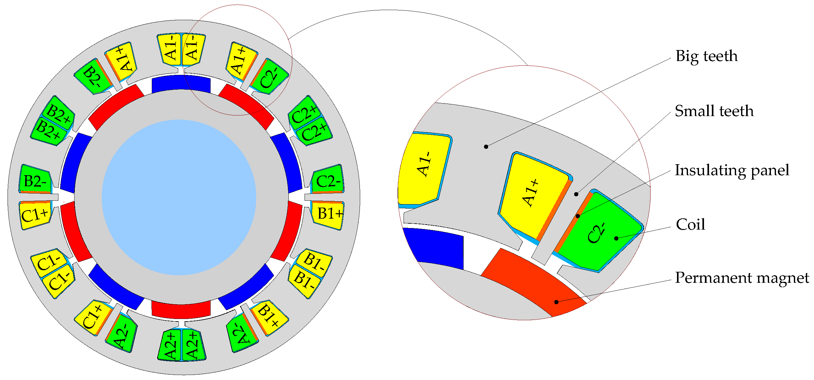
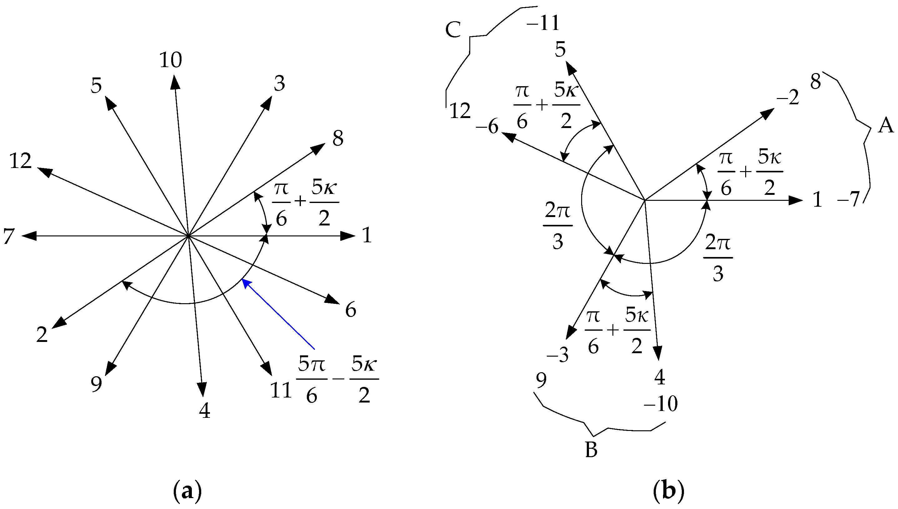
The DRPMSM with weak thermal coupling and no electromagnetic coupling is evolved from the traditional 12 slots, 10 poles three-phase PMSM with fractional-slot concentrated windings [30]. That is to say, small teeth are placed at the center of the slots, in which the two coils belong to different phases. Since the slot leakage flux of coils closes through the small teeth, there is no electromagnetic coupling between two adjacent phase windings. Then, the corresponding mutual inductances are almost zero. The insulating plates are placed on the two sides of the small teeth, which can weaken the thermal coupling between different phase windings. The permanent magnet rotor uses non-equal thickness and tile-shaped permanent magnets which are parallel magnetized. Assuming that the mechanical angle of the small teeth is $\kappa$, the cross-sectional view of DRPMSM, the star graph of the fundamental EMF and the diagram of phase separation, as well as the stator windings outspread diagram of DRPMSM are shown in Figure 1, Figure 2 and Figure 3, respectively.

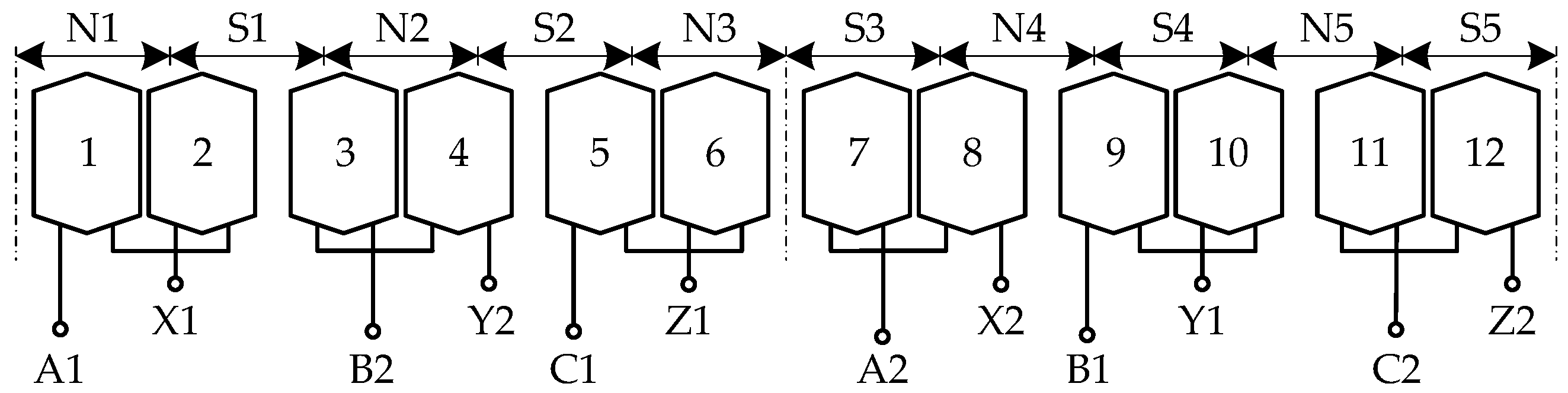
The stator is arranged with six phase windings of A1, B2, C1, A2, B1 and C2. Each phase winding consists of a coil in a forward series connection and a coil in a reverse series connection. The series law of the two coils in the three-phase windings of A1, B1 and C1 is opposite to that of the two coils in the three-phase windings of A2, B2 and C2. The EMF of six phase windings is equal and the phase difference is 120° electrical angle. The resistance and inductance of each phase are the same respectively and the mutual inductance between any two phases is zero. If X1, Y1 and Z1; X2, Y2 and Z2 are connected respectively to form two star points, two independent three-phase star-connected windings A1B1C1 and A2B2C2 are formed. Two sets of three-phase symmetrical windings intersect with each other spatially and are controlled by two inverters fed by one DC power supply.

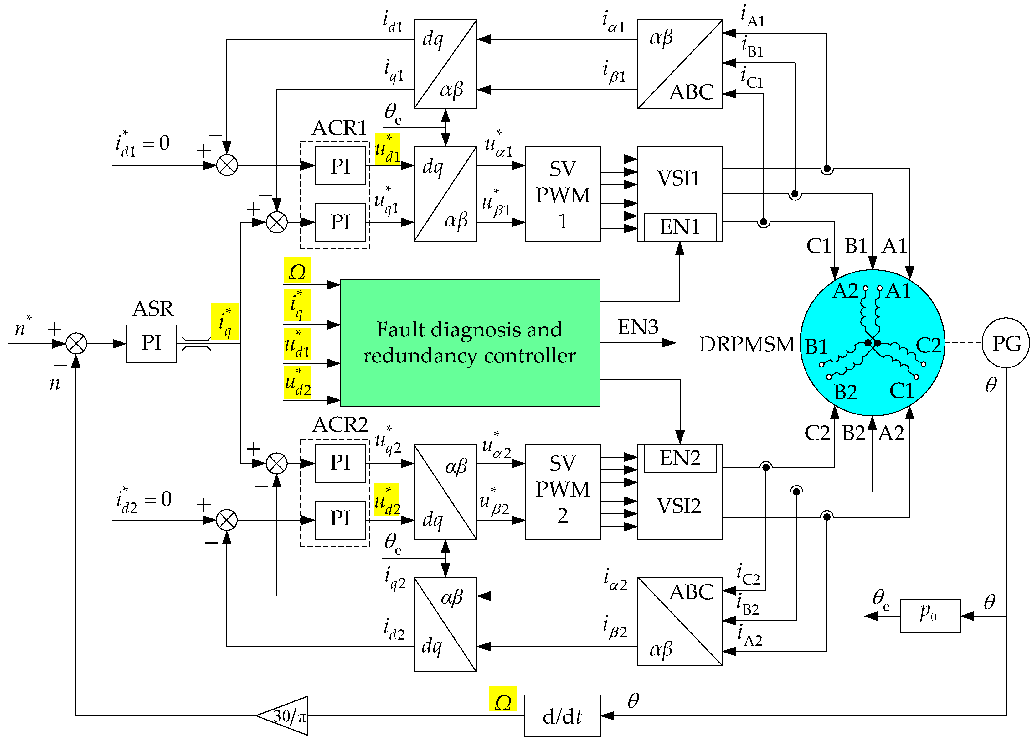
In this paper, the DRPMSM adopts a surface-mounted permanent magnet rotor structure, and the weak magnetic ability of the motor is poor. So the control system of the motor adopts the vector control technology of $i_d^{*}=0$. The output of one speed regulator with PI characteristics is used as q-axis current command of two independent current regulators with PI characteristics. Two current regulators control two sets of windings respectively. $\Omega$, $i_q^{\ast }$, $u_{d1}^{\ast }$, and $u_{d2}^{\ast }$ are mechanical angular velocity, the given q-axis current, the d-axis voltages of the first set of windings and the second set of windings, respectively. They are the inputs of fault diagnosis and redundancy controller, of which $\Omega$ and $i_q^{\ast }$ are used to determine the running modes of the DRPMSM, $u_{d1}^{\ast }$ and $u_{d2}^{\ast }$ are used to determine whether the fault characteristic parameter reach the threshold. The control system block diagram of the DRPMSM is shown in Figure 4.

3. The Mathematical Models and Simulation Models of the DRPMSM

3.1. The Mathematical Models of the DRPMSM under Normal Conditions

Assuming that the ferromagnetic material is unsaturated, the hysteresis loss and eddy current are ignored, and only the fundamental permanent magnetic field is considered. Taking the position where the q-axis of permanent magnet rotor coincides with the axes of the A1 and A2 phase windings as the initial position and taking the counter-clockwise direction as positive direction of permanent magnet rotor, the maximum value of fundamental permanent magnet flux linkage which intersects with each phase winding can be expressed with the following equation:

$${\psi }_{\mathrm{PMm}}=2N_{\mathrm{c}}{k}_{y1}{k}_{q1}{\Phi }_{\mathrm{m}}=2N_{\mathrm{c}}{k}_{w1}{\Phi }_{\mathrm{m}}$$

(1)

where $N_{\mathrm{c}}$ is the number of turns per coil; ${\Phi }_{\mathrm{m}}$ is the fundamental permanent magnetic flux of each pole, and the unit is Wb; $k_{y1}$ is the fundamental pitch-shortening coefficient of coils, $k_{q1}$ is the fundamental distribution coefficient of phase windings; $k_{w1}$ is the fundamental winding coefficient:

$$k_{y1}=k_{q1}=\cos \left(\frac{\mathsf{\pi }}{12}+\frac{5\kappa }{4}\right)$$

(2)

$$k_{w1}=k_{y1}{k}_{q1}={\left[\cos \left(\frac{\mathsf{\pi }}{12}+\frac{5\kappa }{4}\right)\right]}^2$$

(3)

When the DRPMSM operates under normal conditions, the fundamental permanent magnet back EMF of each phase winding can be expressed as follows:

$$e=\left[\begin{array}{l}{e}_{\mathrm{A}1}\\ e_{\mathrm{B}1}\\ e_{\mathrm{C}1}\\ e_{\mathrm{A}2}\\ e_{\mathrm{B}2}\\ e_{\mathrm{C}2}\end{array}\right]=\omega {\psi }_{\mathrm{PMm}}\left[\begin{array}{l}\cos \omega t\\ \cos \left(\omega t-2\mathsf{\pi }/3\right)\\ \cos \left(\omega t-4\mathsf{\pi }/3\right)\\ \cos \omega t\\ \cos \left(\omega t-2\mathsf{\pi }/3\right)\\ \cos \left(\omega t-4\mathsf{\pi }/3\right)\end{array}\right]$$

(4)

where ω is electrical angular velocity of the permanent magnet rotor and the unit is rad/s.

The voltage balance equation can be expressed as follows:

$$\mathit{u}=R\mathit{i}+Lp\mathit{i}+\mathit{e}$$

(5)

where $\mathit{u}$ (V) and $\mathit{i}$ (A) are the column matrices for phase voltage and phase current of two sets of three-phase windings respectively:

$$\mathit{u}={\left[\begin{array}{cccccc}{u}_{\mathrm{A}1}& u_{\mathrm{B}1}& u_{\mathrm{C}1}& u_{\mathrm{A}2}& u_{\mathrm{B}2}& u_{\mathrm{C}2}\end{array}\right]}^{\mathrm{T}}$$

(6)

$$\mathit{i}={\left[\begin{array}{cccccc}{i}_{\mathrm{A}1}& i_{\mathrm{B}1}& i_{\mathrm{C}1}& i_{\mathrm{A}2}& i_{\mathrm{B}2}& i_{\mathrm{C}2}\end{array}\right]}^{\mathrm{T}}$$

(7)

Thus, we can obtain the following expressions:

$$\left[\begin{array}{c}{u}_{\mathrm{A}1}\\ u_{\mathrm{B}1}\\ u_{\mathrm{C}1}\end{array}\right]=R\left[\begin{array}{c}{i}_{\mathrm{A}1}\\ i_{\mathrm{B}1}\\ i_{\mathrm{C}1}\end{array}\right]+L\frac{\mathrm{d}}{\mathrm{d}t}\left[\begin{array}{c}{i}_{\mathrm{A}1}\\ i_{\mathrm{B}1}\\ i_{\mathrm{C}1}\end{array}\right]+\left[\begin{array}{c}{e}_{\mathrm{A}1}\\ e_{\mathrm{B}1}\\ e_{\mathrm{C}1}\end{array}\right]$$

(8)

$$\left[\begin{array}{c}{u}_{\mathrm{A}2}\\ u_{\mathrm{B}2}\\ u_{\mathrm{C}2}\end{array}\right]=R\left[\begin{array}{c}{i}_{\mathrm{A}2}\\ i_{\mathrm{B}2}\\ i_{\mathrm{C}2}\end{array}\right]+L\frac{\mathrm{d}}{\mathrm{d}t}\left[\begin{array}{c}{i}_{\mathrm{A}2}\\ i_{\mathrm{B}2}\\ i_{\mathrm{C}2}\end{array}\right]+\left[\begin{array}{c}{e}_{\mathrm{A}2}\\ e_{\mathrm{B}2}\\ e_{\mathrm{C}2}\end{array}\right]$$

(9)

where R and L represent the resistance and inductance of each phase winding respectively, and the units are Ω and H.

The physical quantities in two sets of three-phase windings are transformed from the three-phase stationary coordinate system to the dq synchronous rotating coordinate system by the power conversation theory, and the voltage Park equations for two sets of windings are given by the following:

$$\left[\begin{array}{c}{u}_{d1}\\ u_{q1}\end{array}\right]=R\left[\begin{array}{c}{i}_{d1}\\ i_{q1}\end{array}\right]+L\frac{\mathrm{d}}{\mathrm{d}t}\left[\begin{array}{c}{i}_{d1}\\ i_{q1}\end{array}\right]+\omega \left[\begin{array}{cc}0& L\\ L& 0\end{array}\right]\left[\begin{array}{c}{i}_{d1}\\ i_{q1}\end{array}\right]+\omega \left[\begin{array}{c}0\\ {\psi }_{\mathrm{f}}\end{array}\right]$$

(10)

$$\left[\begin{array}{c}{u}_{d2}\\ u_{q2}\end{array}\right]=R\left[\begin{array}{c}{i}_{d2}\\ i_{q2}\end{array}\right]+L\frac{\mathrm{d}}{\mathrm{d}t}\left[\begin{array}{c}{i}_{d2}\\ i_{q2}\end{array}\right]+\omega \left[\begin{array}{cc}0& L\\ L& 0\end{array}\right]\left[\begin{array}{c}{i}_{d2}\\ i_{q2}\end{array}\right]+\omega \left[\begin{array}{c}0\\ {\psi }_{\mathrm{f}}\end{array}\right]$$

(11)

$${\psi }_{\mathrm{f}}=\sqrt{3/2}{\psi }_{\mathrm{PMm}}=\sqrt{6}{N}_{\mathrm{c}}{k}_{w1}{\Phi }_{\mathrm{m}}$$

(12)

where $u_d$, $u_q$ are the d-axis voltage and q-axis voltage respectively, and the unit is V; $i_d$, $i_q$ are the d-axis current and q-axis current respectively, and the unit is A; and the subscripts 1 and 2 represent the first set of windings and the second set of windings of the DRPMSM.

Inputting three-phase symmetrical current into two sets of three-phase symmetrical windings, the electromagnetic torque generated by the interaction of armature reaction field and rotor permanent magnetic field is given by the following:

$$T_{\mathrm{e}}=\frac{P_{\mathrm{e}}}{\Omega }=\frac{{\mathit{i}}^{\mathrm{T}}·\mathit{e}}{\omega /p_0}$$

(13)

or:

$$T_{\mathrm{e}}=p_0{\psi }_{\mathrm{f}}\left(i_{q1}+i_{q2}\right)$$

(14)

where $T_{\mathrm{e}}$ is the electromagnetic torque and the unit is $\mathrm{N}·\mathrm{m}$; $P_{\mathrm{e}}$ is the electromagnetic power and the unit is W; $p_0$ is the pole pairs of permanent magnet.

The motion model is given by the following:

$$T_{\mathrm{e}}-T_{\mathrm{L}}=J\frac{\mathrm{d}\Omega }{\mathrm{d}t}+B\Omega$$

(15)

where J is the moment of inertia and the unit is $\mathrm{kg}·{\mathrm{m}}^2$; $T_{\mathrm{L}}$ is the load torque and the unit is $\mathrm{N}·\mathrm{m}$; B is the damping coefficient and the unit is $\mathrm{N}·\mathrm{m}·\mathrm{s}$.

3.2. The Mathematical Models of DRPMSM with an ISCF

3.2.1. Winding Inductances

Firstly, the calculation formulas for magnetizing inductances of the C2 phase winding are derived before and after ISCF occurs.

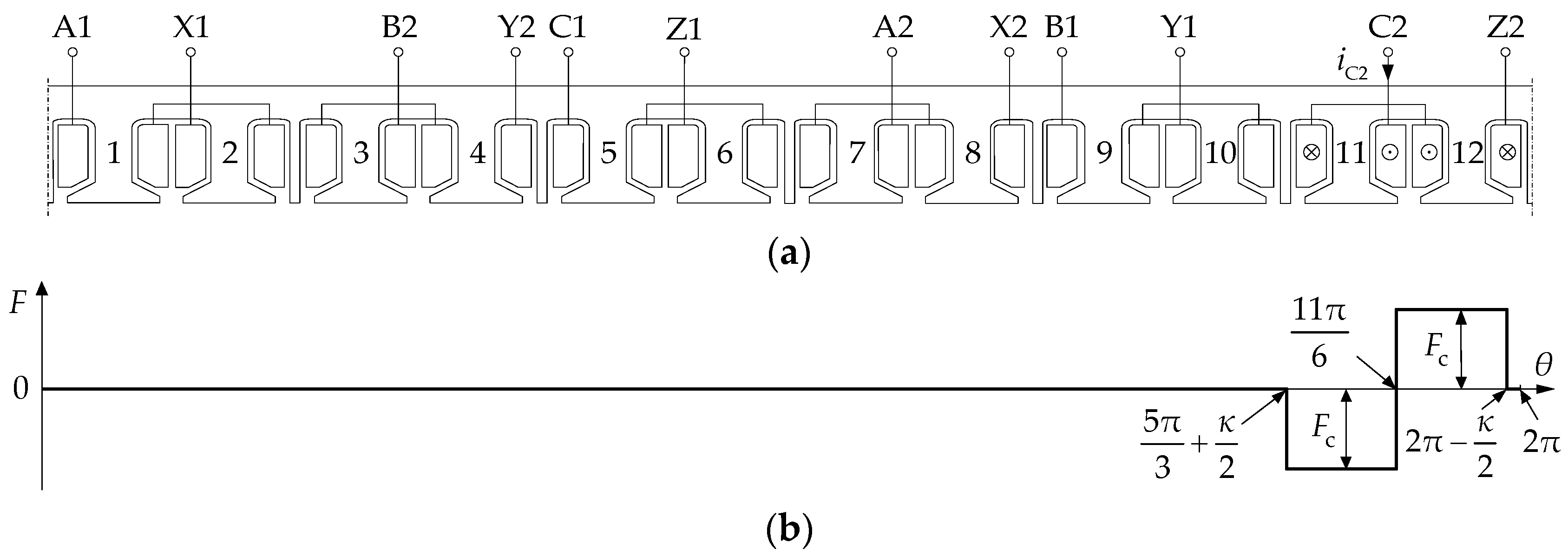
Assuming that only the air-gap magnetomotive force (MMF) exists, the stator winding outspread diagram and the distribution diagram of the MMF generated by C2 phase current ($i_{\mathrm{C}2}$) along the circumference of the air gap under normal conditions are shown in Figure 5. The MMF generated by each normal coil in C2 phase winding can be described by the following equation:

$$F_{\mathrm{c}}=N_{\mathrm{c}}{i}_{\mathrm{C}2}$$

(16)

Ignoring the influence of the stator teeth and slots on the air-gap magnetic permeance, and assuming that the air gap between the stator and the rotor is uniform, the air-gap magnetic permeance per unit area can be expressed as follows:

$${\lambda }_{\mathrm{m}}=\frac{{\mu }_0}{\delta +h_{\mathrm{PM}}}$$

(17)

where ${\mu }_0$ is the permeability of vacuum and ${\mu }_0=4\mathsf{\pi }\times {10}^{-7}\mathrm{H}/\mathrm{m}$; $\delta$ is the length of air gap and the unit is m; $h_{\mathrm{PM}}$ is the radial-magnetized thickness of the surface-mounted permanent magnet and the unit is m.

The flux linkage, which is generated by $i_{\mathrm{C}2}$ and intersects with the C2 phase winding, is given by:

$${\psi }_{\mathrm{C}2\mathrm{C}2}=N_{\mathrm{c}}\left(\frac{\mathsf{\pi }}{3}-\kappa \right)\frac{D_{\mathrm{il}}{l}_{\mathrm{ef}}}{2}{F}_{\mathrm{c}}{\lambda }_{\mathrm{m}}=\frac{\left(\mathsf{\pi }-3\kappa \right)}{6}{N}_{\mathrm{c}}^2{D}_{\mathrm{il}}{l}_{\mathrm{ef}}{\lambda }_{\mathrm{m}}{i}_{\mathrm{C}2}$$

(18)

where $D_{\mathrm{il}}$ is the stator inner diameter, and the unit is m; $l_{\mathrm{ef}}$ is the axial equivalent length of stator core, and the unit is m.

The magnetizing inductance of each phase winding is given by the following:

$$L_{\mathrm{m}}=\frac{{\psi }_{\mathrm{C}2\mathrm{C}2}}{i_{\mathrm{C}2}}=\frac{\left(\mathsf{\pi }-3\kappa \right)}{6}{N}_{\mathrm{c}}^2{D}_{\mathrm{il}}{l}_{\mathrm{ef}}{\lambda }_{\mathrm{m}}$$

(19)

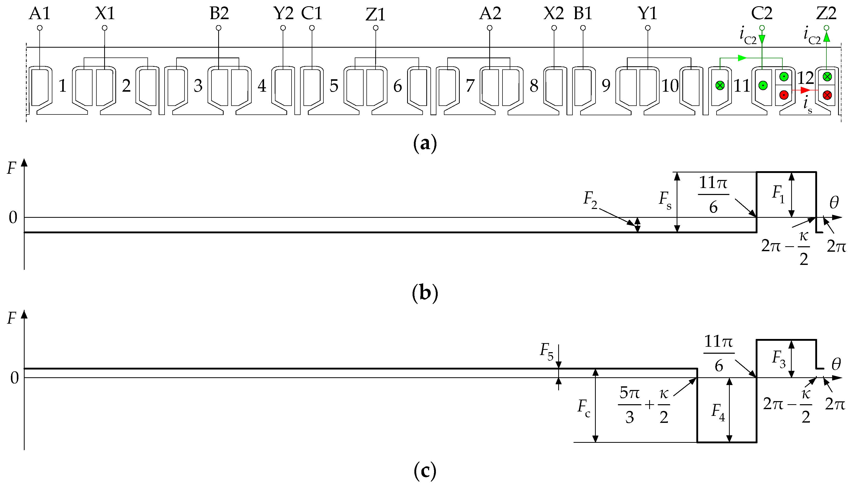
Figure 6 consists of the stator winding outspread diagram when ISCF occurs in coil 12 of the C2 phase winding shown in Figure 3, the distribution diagram of the MMF along the circumference of the air gap generated by the current that passes through the short-circuited turns of coil 12 ($i_{\mathrm{s}}$), and the distribution diagram of the MMF along the circumference of the air gap generated by the current that passes through the C2 phase winding ($i_{\mathrm{C}2}$).

According to the theorem for the conservation of magnetic flux, the magnetic flux of each pole in the uniform air gap is proportional to the area surrounded by the MMF waveform and the horizontal axis. Equation (20) can be deduced from the MMF waveform shown in Figure 6b:

$$\{\begin{array}{l}{F}_1+F_2=F_{\mathrm{s}}=N_{\mathrm{s}}{i}_{\mathrm{s}}\\ \left(\frac{\mathsf{\pi }}{6}-\frac{\kappa }{2}\right)F_1=\left(\frac{11\mathsf{\pi }}{6}+\frac{\kappa }{2}\right)F_2\end{array}$$

(20)

where $N_{\mathrm{s}}$ is the number of short-circuited turns; $F_{\mathrm{s}}$ is the MMF generated by short-circuited turns. Equation (20) can be further simplified as follows:

$$\{\begin{array}{l}{F}_1=\frac{11\mathsf{\pi }+3\kappa }{12\mathsf{\pi }}{N}_{\mathrm{s}}{i}_{\mathrm{s}}\\ F_2=\frac{\mathsf{\pi }-3\kappa }{12\mathsf{\pi }}{N}_{\mathrm{s}}{i}_{\mathrm{s}}\end{array}$$

(21)

Equation (22) can be deduced from the MMF waveform shown in Figure 6c:

$$\{\begin{array}{l}{F}_3-F_5=\left(N_{\mathrm{c}}-N_{\mathrm{s}}\right)i_{\mathrm{C}2}\\ F_4+F_5=N_{\mathrm{c}}{i}_{\mathrm{C}2}\\ \left(\frac{\mathsf{\pi }}{6}-\frac{\kappa }{2}\right)\left(F_4-F_3\right)=\left(\frac{5\mathsf{\pi }}{3}+\kappa \right)F_5\end{array}$$

(22)

Equation (22) can be further simplified as follows:

$$\{\begin{array}{l}{F}_3=\left(N_{\mathrm{c}}-\frac{11\mathsf{\pi }+3\kappa }{12\mathsf{\pi }}{N}_{\mathrm{s}}\right)i_{\mathrm{C}2}\\ F_4=\left(N_{\mathrm{c}}-\frac{\mathsf{\pi }-3\kappa }{12\mathsf{\pi }}{N}_{\mathrm{s}}\right)i_{\mathrm{C}2}\\ F_5=\frac{\mathsf{\pi }-3\kappa }{12\mathsf{\pi }}{N}_{\mathrm{s}}{i}_{\mathrm{C}2}\end{array}$$

(23)

The flux linkage, which is generated by $i_{\mathrm{s}}$ and intersects with the short-circuited turns, is given by the following:

$${\psi }_{\mathrm{ss}}=N_{\mathrm{s}}{F}_1\left(\frac{\mathsf{\pi }}{6}-\frac{\kappa }{2}\right)\frac{D_{\mathrm{il}}{l}_{\mathrm{ef}}}{2}{\lambda }_{\mathrm{m}}=\frac{\left(11\mathsf{\pi }+3\kappa \right)\left(\mathsf{\pi }-3\kappa \right)}{144\mathsf{\pi }}{N}_{\mathrm{s}}^2{D}_{\mathrm{il}}{l}_{\mathrm{ef}}{\lambda }_{\mathrm{m}}{i}_{\mathrm{s}}$$

(24)

The flux linkage, which is generated by $i_{\mathrm{C}2}$ and intersects with the residual normal turns in the C2 phase winding, is given by the following:

$$\begin{array}{ll}{\psi }_{\mathrm{C}2\mathrm{sC}2\mathrm{s}}& =\left[\left(N_{\mathrm{c}}-N_{\mathrm{s}}\right)F_3+N_{\mathrm{c}}{F}_4\right]\left(\frac{\mathsf{\pi }}{6}-\frac{\kappa }{2}\right)\frac{D_{\mathrm{il}}{l}_{\mathrm{ef}}}{2}{\lambda }_{\mathrm{m}}\\ & =\left[\frac{N_{\mathrm{c}}\left(N_{\mathrm{c}}-N_{\mathrm{s}}\right)}{6}+\frac{11\mathsf{\pi }+3\kappa }{144\mathsf{\pi }}{N}_{\mathrm{s}}^2\right]\left(\mathsf{\pi }-3\kappa \right)D_{\mathrm{il}}{l}_{\mathrm{ef}}{\lambda }_{\mathrm{m}}{i}_{\mathrm{C}2}\end{array}$$

(25)

The flux linkage, which is generated by $i_{\mathrm{s}}$ and intersects with the residual normal turns in the C2 phase winding, is given by the following:

$${\psi }_{\mathrm{sC}2\mathrm{s}}=\left[\frac{N_{\mathrm{s}}{N}_{\mathrm{c}}}{12}-\frac{11\mathsf{\pi }+3\kappa }{144\mathsf{\pi }}{N}_{\mathrm{s}}^2\right]\left(\mathsf{\pi }-3\kappa \right)D_{\mathrm{il}}{l}_{\mathrm{ef}}{\lambda }_{\mathrm{m}}{i}_{\mathrm{s}}$$

(26)

Though Equation (24), the magnetizing self-inductance of short-circuited turns can be calculated as follows:

$$L_{\mathrm{mss}}=\frac{{\psi }_{\mathrm{ss}}}{i_{\mathrm{s}}}=\frac{\left(11\mathsf{\pi }+3\kappa \right)\left(\mathsf{\pi }-3\kappa \right)}{144\mathsf{\pi }}{N}_{\mathrm{s}}^2{D}_{\mathrm{il}}{l}_{\mathrm{ef}}{\lambda }_{\mathrm{m}}$$

(27)

Though Equation (25), the magnetizing self-inductance of residual normal turns in the C2 phase winding can be calculated as follows:

$$L_{\mathrm{mC}2\mathrm{sC}2\mathrm{s}}=\frac{{\psi }_{\mathrm{C}2\mathrm{sC}2\mathrm{s}}}{i_{\mathrm{C}2}}=\left[\frac{N_{\mathrm{c}}\left(N_{\mathrm{c}}-N_{\mathrm{s}}\right)}{6}+\frac{11\mathsf{\pi }+3\kappa }{144\mathsf{\pi }}{N}_{\mathrm{s}}^2\right]\left(\mathsf{\pi }-3\kappa \right)D_{\mathrm{il}}{l}_{\mathrm{ef}}{\lambda }_{\mathrm{m}}$$

(28)

Though Equation (26), the magnetizing mutual inductance between short-circuited turns and residual normal turns in the C2 phase winding can be calculated as follows:

$$M_{\mathrm{msC}2\mathrm{s}}=\frac{{\psi }_{\mathrm{sC}2\mathrm{s}}}{i_{\mathrm{s}}}=\left[\frac{N_{\mathrm{s}}{N}_{\mathrm{c}}}{12}-\frac{11\mathsf{\pi }+3\kappa }{144\mathsf{\pi }}{N}_{\mathrm{s}}^2\right]\left(\mathsf{\pi }-3\kappa \right)D_{\mathrm{il}}{l}_{\mathrm{ef}}{\lambda }_{\mathrm{m}}$$

(29)

Besides, there are also end winding leakage inductances and slot leakage inductances in the C2 phase winding. The end winding leakage inductance of the C2 phase winding under normal conditions can be given by the following equation:

$$L_{\sigma \mathrm{E}}=0.8{\mu }_0{N}_{\mathrm{c}}^2{l}_{\mathrm{E}}$$

(30)

where $l_{\mathrm{E}}$ is the end winding length of a half-turn coil, and the unit is m.

After the ISFC occurs, the end winding leakage self-inductance of short-circuited turns can be given by the following equation:

$$L_{\sigma \mathrm{Es}}=0.4{\mu }_0{N}_{\mathrm{s}}^2{l}_{\mathrm{E}}$$

(31)

The end winding leakage self-inductance of residual normal turns in the C2 phase winding can be given by the following:

$$L_{\sigma \mathrm{EC}2\mathrm{s}}=0.4{\mu }_0\left[{\left(N_{\mathrm{c}}-N_{\mathrm{s}}\right)}^2+N_{\mathrm{c}}^2\right]l_{\mathrm{E}}$$

(32)

The end winding leakage mutual inductance between short-circuited turns and residual normal turns in the short-circuited coil can be given by the following:

$$M_{\sigma \mathrm{EsC}2\mathrm{s}}=0.4{\mu }_0{N}_{\mathrm{s}}\left(N_{\mathrm{c}}-N_{\mathrm{s}}\right)l_{\mathrm{E}}$$

(33)

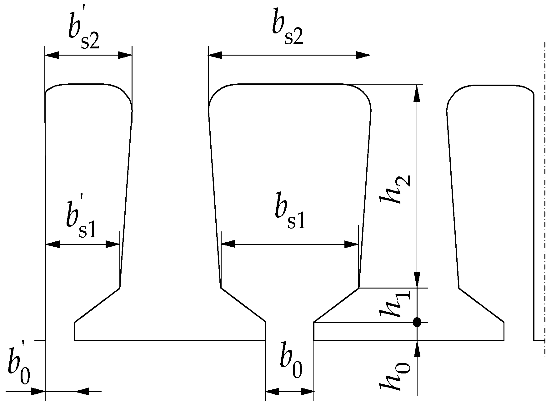
The slot leakage inductances which are determined by slot leakage permeance are relatively large. The slot leakage permeance is closely related to the size of the stator slots. The shape of the stator slots in which a phase winding can be embedded is shown in Figure 7.

When coils are normal, the slot leakage inductance $L_{\mathsf{\sigma }\mathrm{S}}$ of each phase winding includes the slot leakage self-inductances for the edges of two coils in a big slot, the slot leakage mutual inductances between the edges of two coils in a big slot and the slot leakage self-inductances for the edges of two coils in two small slots. In other words:

$$L_{\mathsf{\sigma }\mathrm{S}}={\mu }_0{l}_{\mathrm{ef}}{N}_{\mathrm{c}}^2[4\left(\frac{2h_2}{3\left(b_{\mathrm{s}1}+b_{\mathrm{s}2}\right)}+\frac{2h_1}{b_0+b_{\mathrm{s}1}}+\frac{h_0}{b_0}\right)+2\left(\frac{2h_2}{3\left(b_{\mathrm{s}1}^{\prime }+b_{\mathrm{s}2}^{\prime }\right)}+\frac{2h_1}{b_0^{\prime }+b_{\mathrm{s}1}^{\prime }}+\frac{h_0}{b_0^{\prime }}\right)]$$

(34)

When the ISCF occurs, the slot leakage inductance $L_{\mathsf{\sigma }\mathrm{Ss}}$ of short-circuited turns includes the slot leakage self-inductances for the edges of short-circuited turns in a big slot and a small slot. That is:

$$L_{\mathsf{\sigma }\mathrm{Ss}}={\mu }_0{l}_{\mathrm{ef}}{N}_{\mathrm{s}}^2[\left(\frac{2h_2}{3\left(b_{\mathrm{s}1}+b_{\mathrm{s}2}\right)}+\frac{2h_1}{b_0+b_{\mathrm{s}1}}+\frac{h_0}{b_0}\right)+\left(\frac{2h_2}{3\left(b_{\mathrm{s}1}^{\prime }+b_{\mathrm{s}2}^{\prime }\right)}+\frac{2h_1}{b_0^{\prime }+b_{\mathrm{s}1}^{\prime }}+\frac{h_0}{b_0^{\prime }}\right)]$$

(35)

The slot leakage inductance $L_{\mathsf{\sigma }\mathrm{SC}2\mathrm{s}}$ of residual normal turns in the C2 phase winding contains the slot leakage self-inductances of a normal coil edges in a big slot and a small slot, the slot leakage self-inductances for the edges of residual normal turns belonging to the short-circuited coil in a big slot and a small slot, the slot leakage mutual inductances between a normal coil edges and the edges of residual normal turns belonging to the short-circuited coil in a big slot. That is:

$$\begin{array}{cc}\hfill L_{\mathsf{\sigma }\mathrm{SC}2\mathrm{s}}=& {\mu }_0{l}_{\mathrm{ef}}\{\left[N_{\mathrm{c}}^2+{\left(N_{\mathrm{c}}-N_{\mathrm{s}}\right)}^2\right]\left[\left(\frac{2h_2}{3\left(b_{\mathrm{s}1}+b_{\mathrm{s}2}\right)}+\frac{2h_1}{b_0+b_{\mathrm{s}1}}+\frac{h_0}{b_0}\right)+\left(\frac{2h_2}{3\left(b_{\mathrm{s}1}^{\prime }+b_{\mathrm{s}2}^{\prime }\right)}+\frac{2h_1}{b_0^{\prime }+b_{\mathrm{s}1}^{\prime }}+\frac{h_0}{b_0^{\prime }}\right)\right]\hfill \\ & +2\left[N_{\mathrm{c}}\left(N_{\mathrm{c}}-N_{\mathrm{s}}\right)\right]\left(\frac{2h_2}{3\left(b_{\mathrm{s}1}+b_{\mathrm{s}2}\right)}+\frac{2h_1}{b_0+b_{\mathrm{s}1}}+\frac{h_0}{b_0}\right)\}\hfill \end{array}$$

(36)

The slot leakage mutual inductance $M_{\mathsf{\sigma }\mathrm{SsC}2\mathrm{s}}$ between short-circuited turns and residual normal turns in the C2 phase winding contains the slot leakage mutual inductance between the edges of short-circuited turns and a normal coil edges in a big slot, the slot leakage mutual inductance between the edges of short-circuited turns and the edges of residual normal turns belonging to the short-circuited coil in a big slot, and the slot leakage mutual inductance between the edges of short-circuited turns and the edges of residual normal turns belonging to the short-circuited coil in a small slot. That is:

$$\begin{array}{c}{M}_{\mathsf{\sigma }\mathrm{SsC}2\mathrm{s}}={\mu }_0{l}_{\mathrm{ef}}{N}_{\mathrm{s}}\{\left[N_{\mathrm{c}}+\left(N_{\mathrm{c}}-N_{\mathrm{s}}\right)\right]\left(\frac{2h_2}{3\left(b_{\mathrm{s}1}+b_{\mathrm{s}2}\right)}+\frac{2h_1}{b_0+b_{\mathrm{s}1}}+\frac{h_0}{b_0}\right)+\\ \left(N_{\mathrm{c}}-N_{\mathrm{s}}\right)\left(\frac{2h_2}{3\left(b_{\mathrm{s}1}^{\prime }+b_{\mathrm{s}2}^{\prime }\right)}+\frac{2h_1}{b_0^{\prime }+b_{\mathrm{s}1}^{\prime }}+\frac{h_0}{b_0^{\prime }}\right)\}\end{array}$$

(37)

with the above analysis, the full self-inductance L of a phase winding is given by:

$$L=L_{\mathrm{m}}+L_{\sigma \mathrm{E}}+L_{\sigma \mathrm{S}}$$

(38)

The full self-inductance $L_{\mathrm{s}}$ of short-circuited turns is given by:

$$L_{\mathrm{s}}=L_{\mathrm{mss}}+L_{\sigma \mathrm{Es}}+L_{\sigma \mathrm{Ss}}$$

(39)

The full self-inductance $L_{\mathrm{C}2\mathrm{s}}$ of residual normal turns in the C2 phase winding is given by:

$$L_{\mathrm{C}2\mathrm{s}}=L_{\mathrm{mC}2\mathrm{sC}2\mathrm{s}}+L_{\sigma \mathrm{EC}2\mathrm{s}}+L_{\sigma \mathrm{SC}2\mathrm{s}}$$

(40)

The full mutual inductance $M_{\mathrm{sC}2\mathrm{s}}$ between short-circuited turns and residual normal turns in the C2 phase winding is given by:

$$M_{\mathrm{sC}2\mathrm{s}}=M_{\mathrm{msC}2\mathrm{s}}+M_{\sigma \mathrm{EsC}2\mathrm{s}}+M_{\sigma \mathrm{SsC}2\mathrm{s}}$$

(41)

Finally, the resistances of short-circuited turns and residual normal turns in the C2 phase winding can be respectively written as follows:

$$R_{\mathrm{s}}=\frac{N_{\mathrm{s}}}{2N_{\mathrm{c}}}R$$

(42)

$$R_{\mathrm{C}2\mathrm{s}}=\left(1-\frac{N_{\mathrm{s}}}{2N_{\mathrm{c}}}\right)R$$

(43)

3.2.2. The Mathematical Models of the DRPMSM

Assuming that the first set of three-phase windings is normal, and the ISCF occurs in coil 12 of the C2 phase winding which belongs to the second set of three-phase windings in the DRPMSM, the voltage equations of the first set of normal three-phase windings remain unchanged and can be expressed as Equation (8). Thus, the following discussions only focus on the second set of three-phase windings.

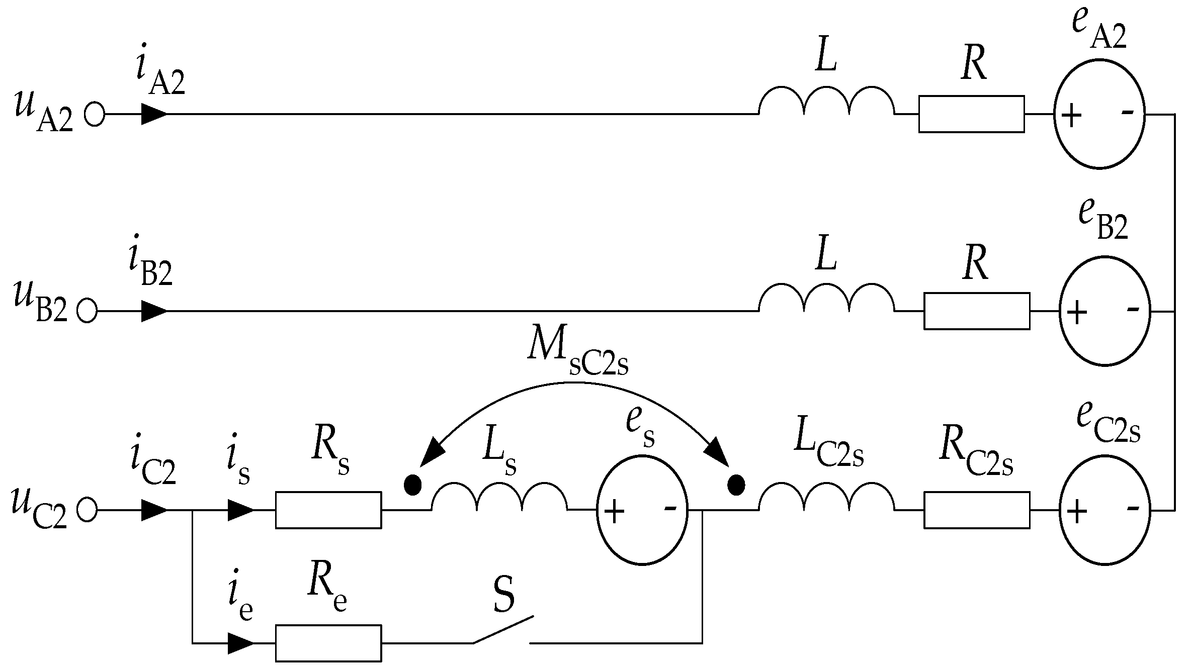
Utilizing an external contact resistance $R_{\mathrm{e}}$, the imitation for the ISCF can be realized. The equivalent circuit diagram of the second set of windings is shown in Figure 8.

The circuit parameters of the C2 phase winding in Figure 8 can be expressed as follows:

$$R_{\mathrm{s}}+R_{\mathrm{C}2\mathrm{s}}=R$$

(44)

$$L_{\mathrm{s}}+L_{\mathrm{C}2\mathrm{s}}+2M_{\mathrm{sC}2\mathrm{s}}=L$$

(45)

$$e_{\mathrm{s}}+e_{\mathrm{C}2\mathrm{s}}=e_{\mathrm{C}2}$$

(46)

$$e_{\mathrm{s}}=\omega N_{\mathrm{s}}{k}_{\mathrm{y}1}{\Phi }_{\mathrm{m}}\cos \left[\omega t-5\left(\mathsf{\pi }-\kappa \right)/4\right]$$

(47)

$$e_{\mathrm{C}2\mathrm{s}}=\omega k_{y1}{\Phi }_{\mathrm{m}}\{\left(N_{\mathrm{c}}-N_{\mathrm{s}}\right)\cos \left[\omega t-5\left(\mathsf{\pi }-\kappa \right)/4\right]+N_{\mathrm{c}}\cos \left[\omega t-\left(17\mathsf{\pi }+15\kappa \right)/12\right]\}$$

(48)

where $R_{\mathrm{s}}$ and $R_{\mathrm{C}2\mathrm{s}}$, $L_{\mathrm{s}}$ and $L_{\mathrm{C}2\mathrm{s}}$, $e_{\mathrm{s}}$ and $e_{\mathrm{C}2\mathrm{s}}$ represent the resistances, inductances and permanent magnet back EMFs of short-circuited turns and residual normal turns in the C2 phase winding, respectively.

When the short circuit switch S is open, the second set of three-phase windings is normal and its voltage equations are the same as Equation (9). When the short circuit switch S is closed, the ISCF occurs. In this case, the voltage equations of the A2 and B2 phase windings are still as shown by Equation (9). The voltage and current equations of short-circuited turns and residual normal turns in the C2 phase winding can be obtained based on the positive direction shown in Figure 8:

$$i_{\mathrm{e}}{R}_{\mathrm{e}}=i_{\mathrm{s}}{R}_{\mathrm{s}}+L_{\mathrm{s}}\frac{\mathrm{d}{i}_{\mathrm{s}}}{\mathrm{d}t}+M_{\mathrm{sC}2\mathrm{s}}\frac{\mathrm{d}{i}_{\mathrm{C}2}}{\mathrm{d}t}+e_{\mathrm{s}}$$

(49)

$$u_{\mathrm{C}2}=i_{\mathrm{e}}{R}_{\mathrm{e}}+L_{\mathrm{C}2\mathrm{s}}\frac{\mathrm{d}{i}_{\mathrm{C}2}}{\mathrm{d}t}+M_{\mathrm{sC}2\mathrm{s}}\frac{\mathrm{d}{i}_{\mathrm{s}}}{\mathrm{d}t}+i_{\mathrm{C}2}{R}_{\mathrm{C}2\mathrm{s}}+e_{\mathrm{C}2\mathrm{s}}$$

(50)

$$i_{\mathrm{C}2}=i_{\mathrm{s}}+i_{\mathrm{e}}$$

(51)

The electromagnetic torque is given by:

$$T_{\mathrm{e}}=\frac{P_{\mathrm{e}}}{\Omega }=\frac{p_0}{\omega }[\left(i_{\mathrm{A}1}{e}_{\mathrm{A}1}+i_{\mathrm{B}1}{e}_{\mathrm{B}1}+i_{\mathrm{C}1}{e}_{\mathrm{C}1}\right)+\left(i_{\mathrm{A}2}{e}_{\mathrm{A}2}+i_{\mathrm{B}2}{e}_{\mathrm{B}2}+i_{\mathrm{C}2}{e}_{\mathrm{C}2\mathrm{s}}+i_{\mathrm{s}}{e}_{\mathrm{s}}\right)]$$

(52)

3.3. The Simulation Models of the DRPMSM

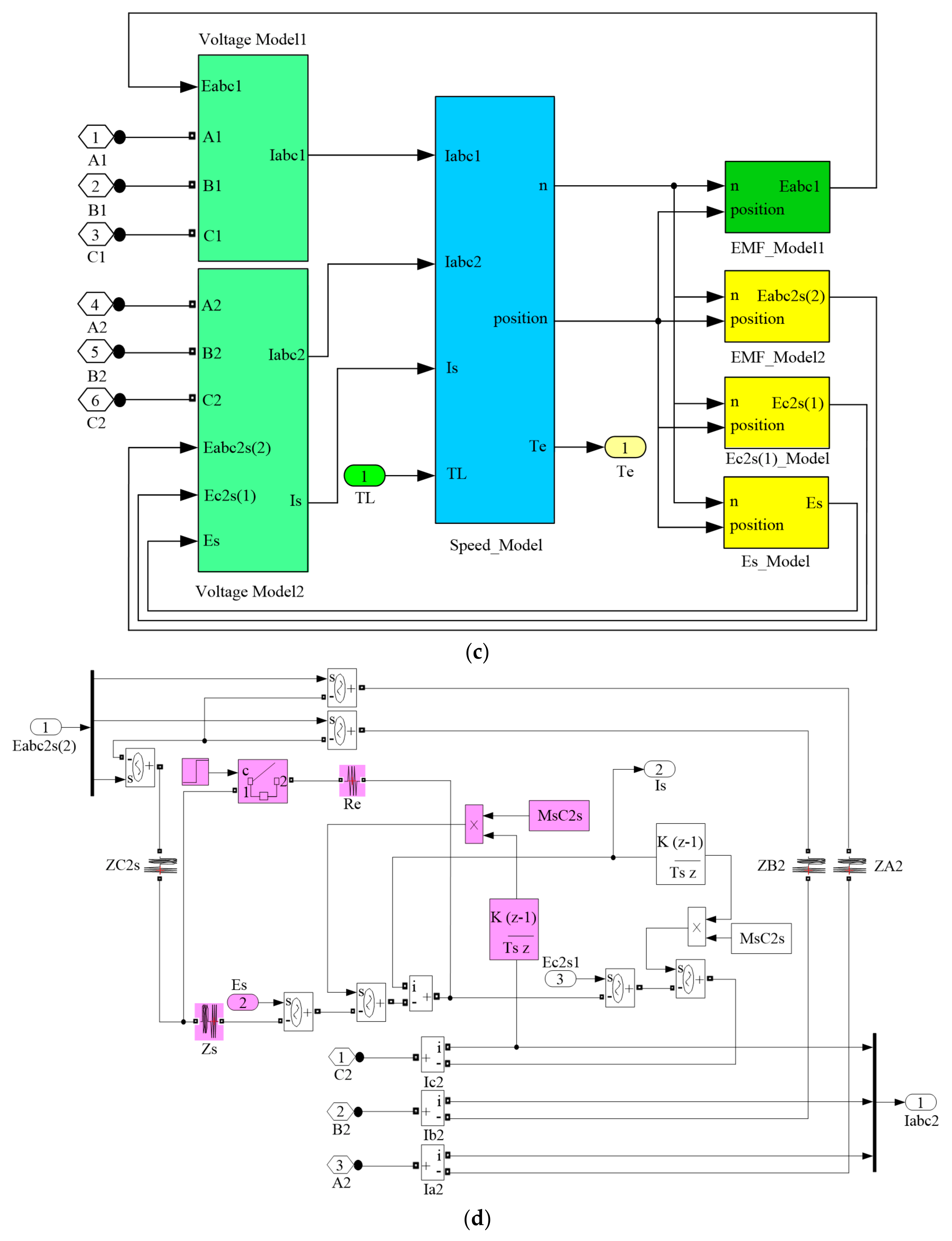
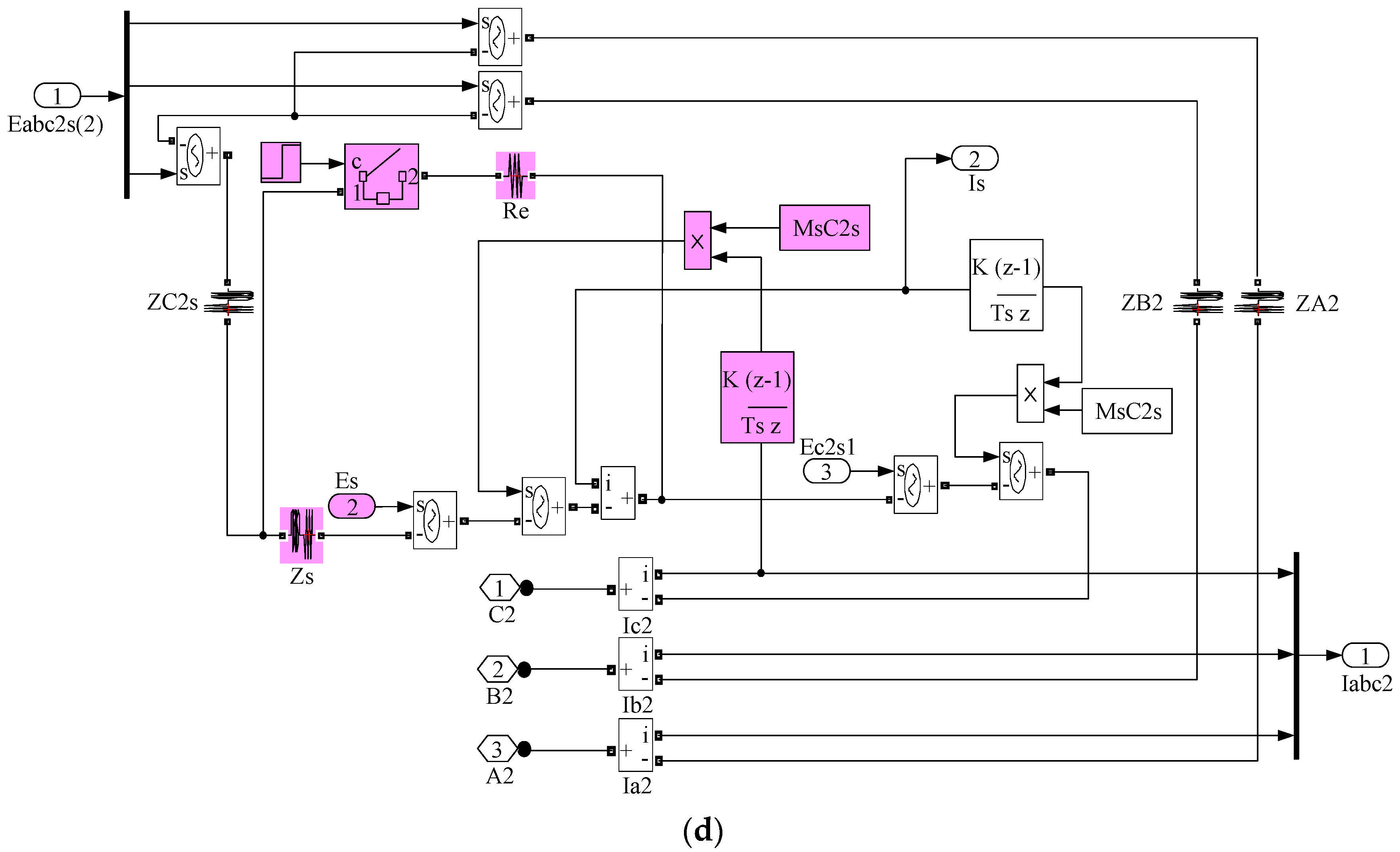
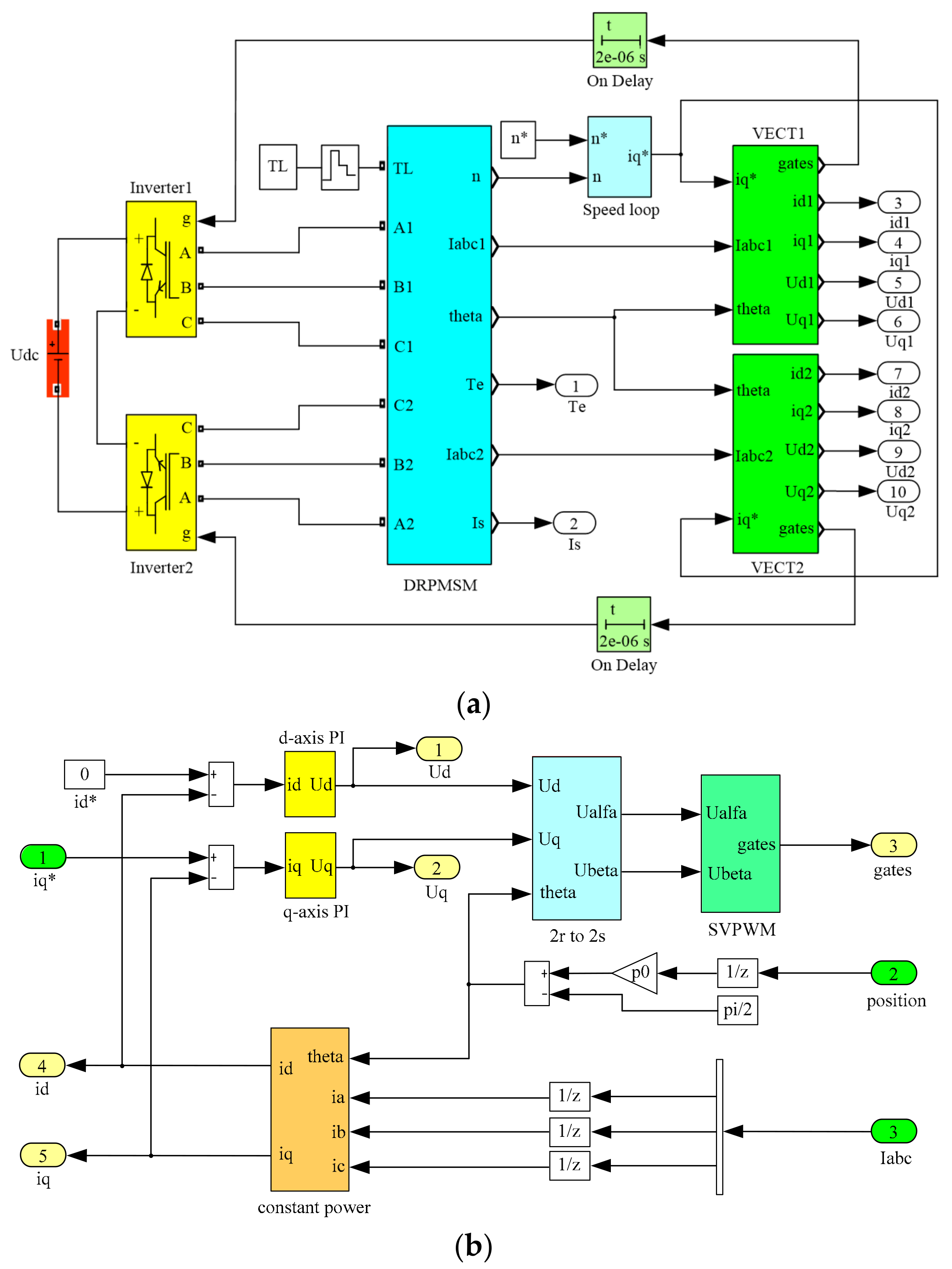
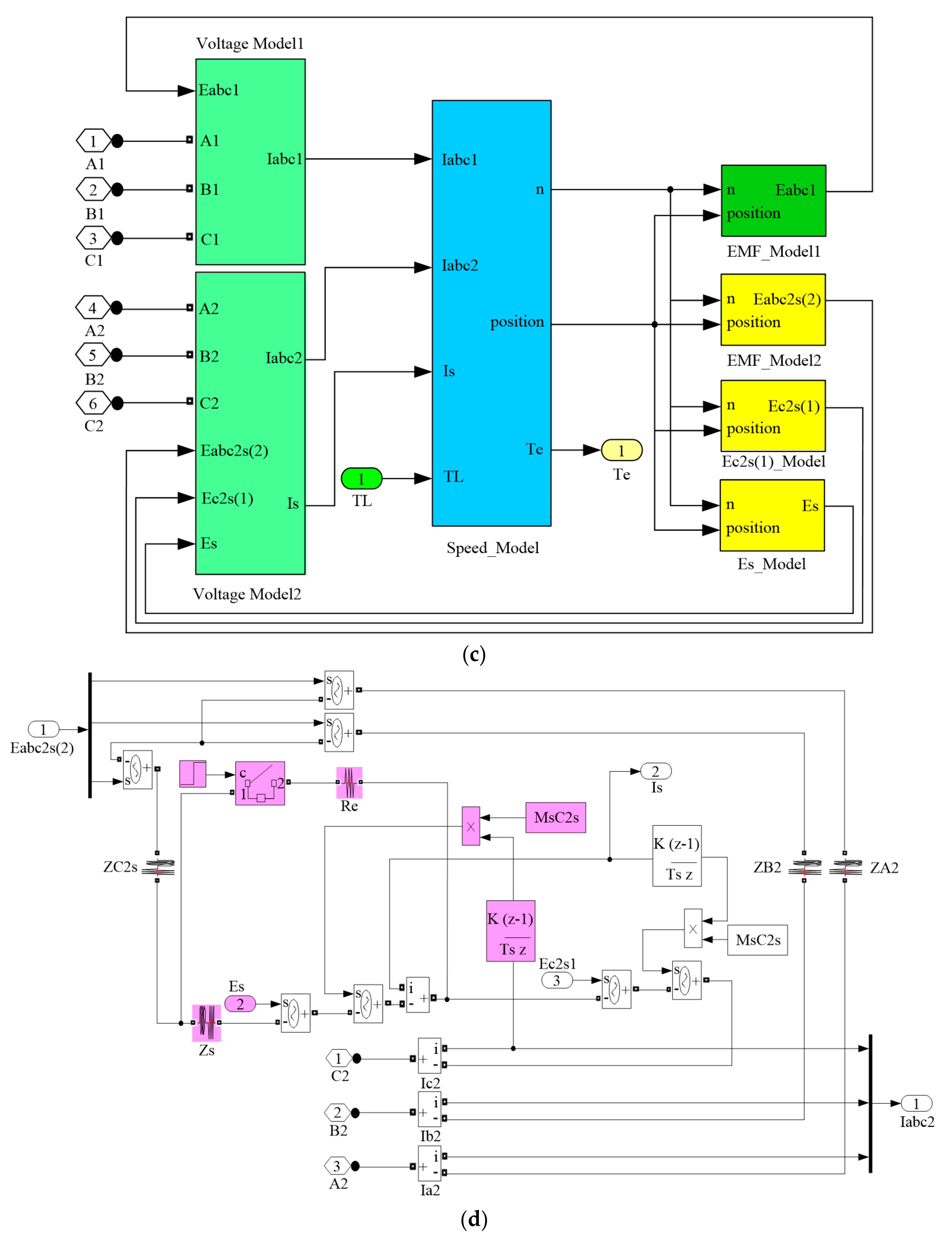
The simulation models of an ISCF in a DRPMSM are built on the MATLAB R2014a/Simulink platform. The sampling frequency and the solver are set to 10 kHz and ode45, respectively. The simulation model of the overall control system for the motor, the sub-models of the vector control system, the DRPMSM and the set of faulty windings are shown in Figure 9, respectively. After ISCF occurs, the models of the vector control systems for two sets of windings are the same, but the models of windings structures and permanent magnet back EMFs for two redundancies are different.

4. The Simulation Analyses and Online Diagnosis of an ISCF in DRPMSM

4.1. The Simulation Analyses of the DRPMSM

The main parameters of the DRPMSM are shown in

Table 1. Parameters of the DRPMSM.

Parameters	Value
Rated power $P_{\mathrm{N}}$	3.5 kW
Rated speed $n_{\mathrm{N}}$	1200 r/min
Rated current $I_{\mathrm{N}}$	17.7 A
Rated torque $T_{\mathrm{N}}$	26.5 N·m
DC supply voltage $U_{\mathrm{dc}}$	200 V
Phase inductance $L$	2.19 mH
Phase resistance $R$	0.157 Ω
Permanent magnet flux linkage ${\psi }_{\mathrm{f}}$	0.094 Wb
Moment of inertia $J$	0.055 kg·m2
Coil turns number $N_{\mathrm{c}}$	25
Number of pole pairs $p_0$	5

.

According to the simulation models and motor parameters, a series of simulation analyses are carried out.

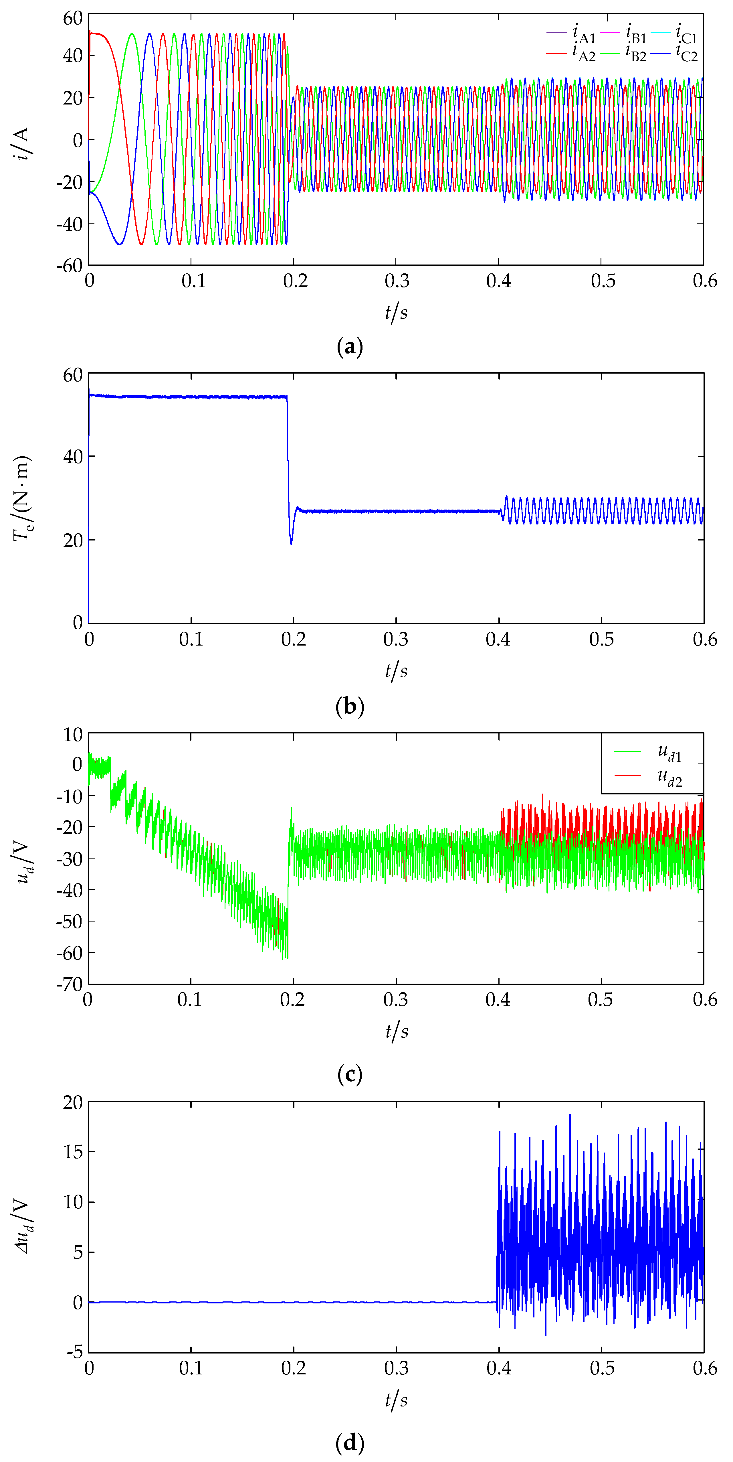
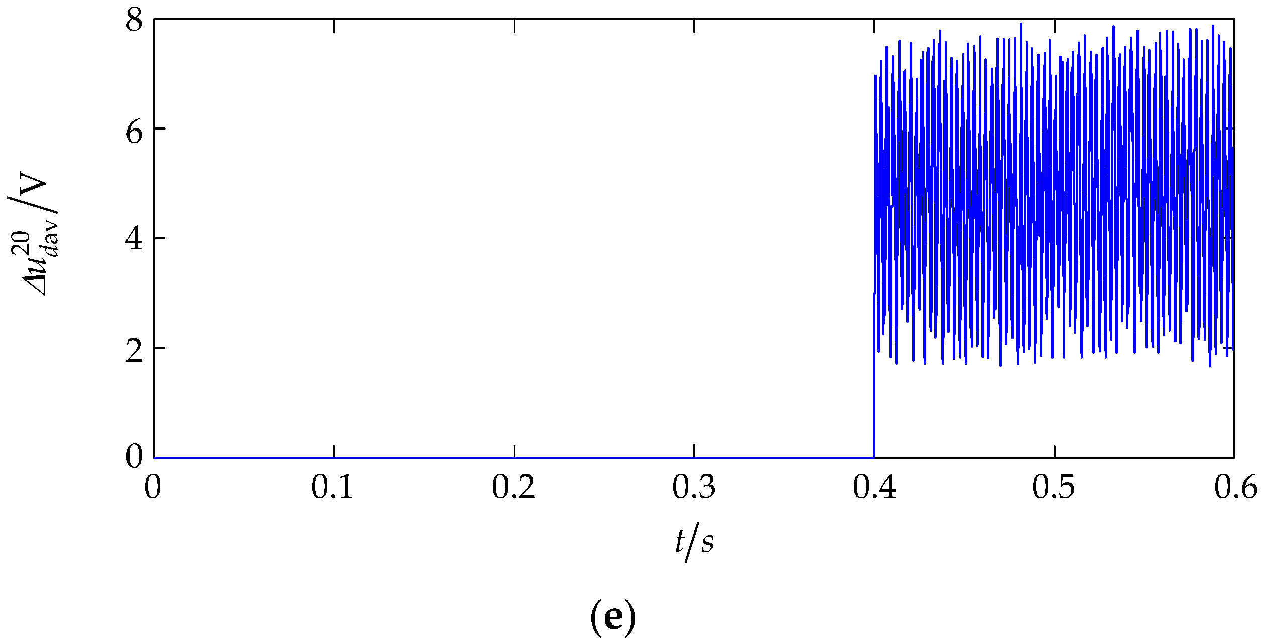
Supposing that the motor starts normally with a rated load, the given speed $n^{\ast }$ is set to 900 r/min. When t = 0.4 s, the ISCF occurs. The external contact resistance and the number of short-circuited turns are set to 0.1 Ω and 10, respectively. The simulation time is 0.6 s. The simulation results are shown in Figure 10, which include the three phase currents of two sets of windings, the electromagnetic torque, the d-axis voltages of two sets of windings, the difference of the d-axis voltages between the set of faulty windings and the set of normal windings and the average values for the difference of the d-axis voltages in the latest 20 sampling periods.

As shown in Figure 10, the three phase currents of two sets of windings are almost identical before and after the ISCF occurs. When the motor is normal, two sets of three-phase windings are identical, so the three phase currents of two sets of windings are identical naturally. After the ISCF occurs, the double-frequency component of electromagnetic torque increases significantly. The structures and permanent magnet back EMFs of two sets of windings are different. However, the control systems of two sets of windings are controlled by one speed regulator, that is, the inputs of the current regulators for two sets of windings are the same. Besides, the adjusting speed of the current regulator is extremely fast, so the three phase currents of two sets of windings produce almost the same distortion. In general, whether the motor is normal or has a coil ISCF, the following equations are satisfied:

$$\left[\begin{array}{c}{i}_{\mathrm{A}1}\\ i_{\mathrm{B}1}\\ i_{\mathrm{C}1}\end{array}\right]\approx \left[\begin{array}{c}{i}_{\mathrm{A}2}\\ i_{\mathrm{B}2}\\ i_{\mathrm{C}2}\end{array}\right]$$

(53)

$$\left[\begin{array}{c}{i}_{d1}\\ i_{q1}\end{array}\right]\approx \left[\begin{array}{c}{i}_{d2}\\ i_{q2}\end{array}\right]\approx \left[\begin{array}{c}{i}_d\\ i_q\end{array}\right]$$

(54)

Therefore, according to the three phase currents of two sets of windings, the existence of an ISCF could be diagnosed, but the set of faulty windings cannot be determined.

4.2. The Online Detection of an ISCF

After an ISCF occurs, the equivalent resistance and inductance in the voltage Park equation of the second set of windings are reduced by $\Delta R$ and $\Delta L$, respectively. The d-axis voltages of two sets of windings are:

$$u_{d1}=R{i}_{d1}+L\frac{\mathrm{d}{i}_{d1}}{\mathrm{d}t}-\omega L{i}_{q1}$$

(55)

$$u_{d2}=\left(R-\Delta R\right)i_{d2}+\left(L-\Delta L\right)\frac{\mathrm{d}{i}_{d2}}{\mathrm{d}t}-\omega \left(L-\Delta L\right)i_{q2}$$

(56)

The difference of the d-axis voltages between the set of faulty windings and the set of normal windings ($\Delta u_d$) can be acquired by subtracting Equation (55) from Equation (56):

$$\Delta u_d=u_{d2}-u_{d1}\approx -i_{d2}\Delta R-\frac{\mathrm{d}{i}_{d2}}{\mathrm{d}t}\Delta L+\omega i_{q2}\Delta L$$

(57)

Since $i_d^{*}=0$, the d-axis current is basically maintained at 0 and changes slightly between positive and negative values. As shown in Equation (57), when the motor runs steadily, $i_d\Delta R$ is about zero, $\Delta L\left(\mathrm{d}{i}_d/\mathrm{d}t\right)$ changes between positive and negative values, and $\omega i_q\Delta L$ is a finite value.

$\Delta u_d$ can be acquired in each sampling period of the digital signal processor (DSP). Averaging $\Delta u_d$ in the latest K sampling periods has the same effect as the digital average filtering for $\Delta u_d$. When K becomes relatively large, the following equations can be obtained:

$$\frac{1}{K}{\displaystyle \sum _{k=1}^K{i}_d\left(k\right)\Delta R}\approx 0$$

(58)

$$\frac{\Delta L}{K}{\displaystyle \sum _{k=1}^K\frac{i_d\left(k\right)-i_d\left(k-1\right)}{{\tau }_{\mathrm{sample}}}}=\frac{\Delta L}{K}\frac{i_d\left(K\right)-i_d\left(0\right)}{{\tau }_{\mathrm{sample}}}=\epsilon$$

(59)

$$\Delta u_{d\mathrm{av}}^K=\frac{1}{K}\Delta u_{d\mathsf{\Sigma }}=\frac{1}{K}{\displaystyle \sum _{k=1}^K\Delta u_d\left(k\right)}=\frac{\Delta L}{K}{\displaystyle \sum _{k=1}^K\omega \left(k\right)i_q\left(k\right)}+\epsilon$$

(60)

where ${\tau }_{\mathrm{sample}}$ represents the current sampling period, which is the same as the control cycle of pulse width modulation (PWM); $\Delta u_{d\mathrm{av}}^K$ represent the average values for the difference of the d-axis voltages between the set of faulty windings and the set of normal windings in the latest K sampling periods, and the unit is V.

It can be ascertained from Equation (60) that $\Delta u_{d\mathrm{av}}^K$ mainly depend on the electrical angular velocity and the q-axis current in the latest K sampling periods. $\Delta u_{d\mathrm{av}}^K$ are $\Delta u_{d\mathrm{av}}^{20}$ when sampling periods are 20. The absolute value of $\Delta u_{d\mathrm{av}}^K$, i.e., $\left|\Delta u_{d\mathrm{av}}^K\right|$ are fault characteristic parameters.

As shown in Figure 10, when the motor is normal, the d-axis voltages of two sets of windings are basically identical; $\Delta u_d$ and $\Delta u_{d\mathrm{av}}^{20}$ are about zero. When an ISCF occurs, there are deviations in the d-axis voltages of two sets of windings. Further, most of $\Delta u_d$ are greater than zero and $\Delta u_{d\mathrm{av}}^{20}$ are greater than 1 V. Thus, the set of faulty windings can be detected online by observing $\Delta u_{d\mathrm{av}}^{20}$ when the motor runs under stable conditions.

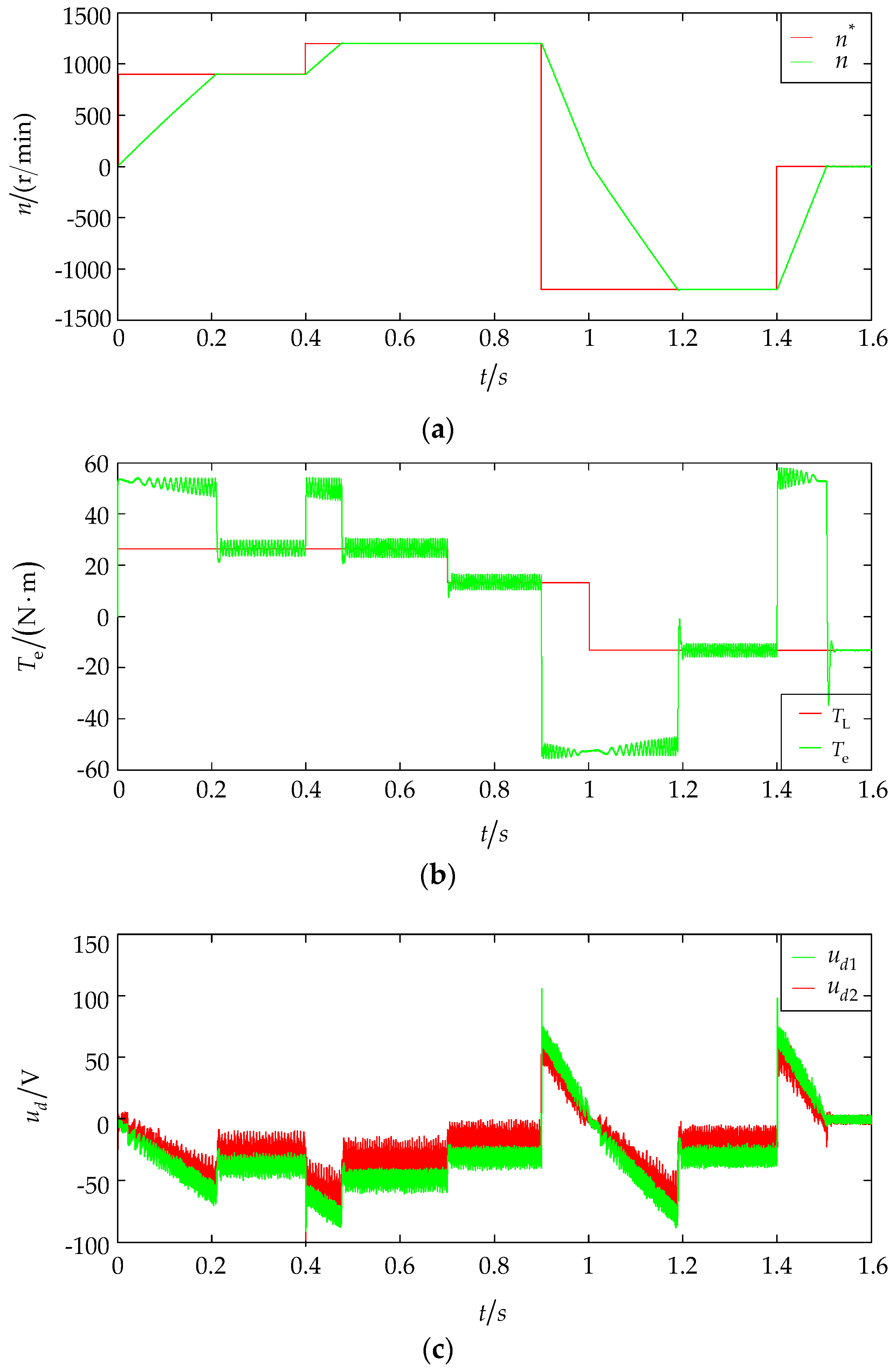
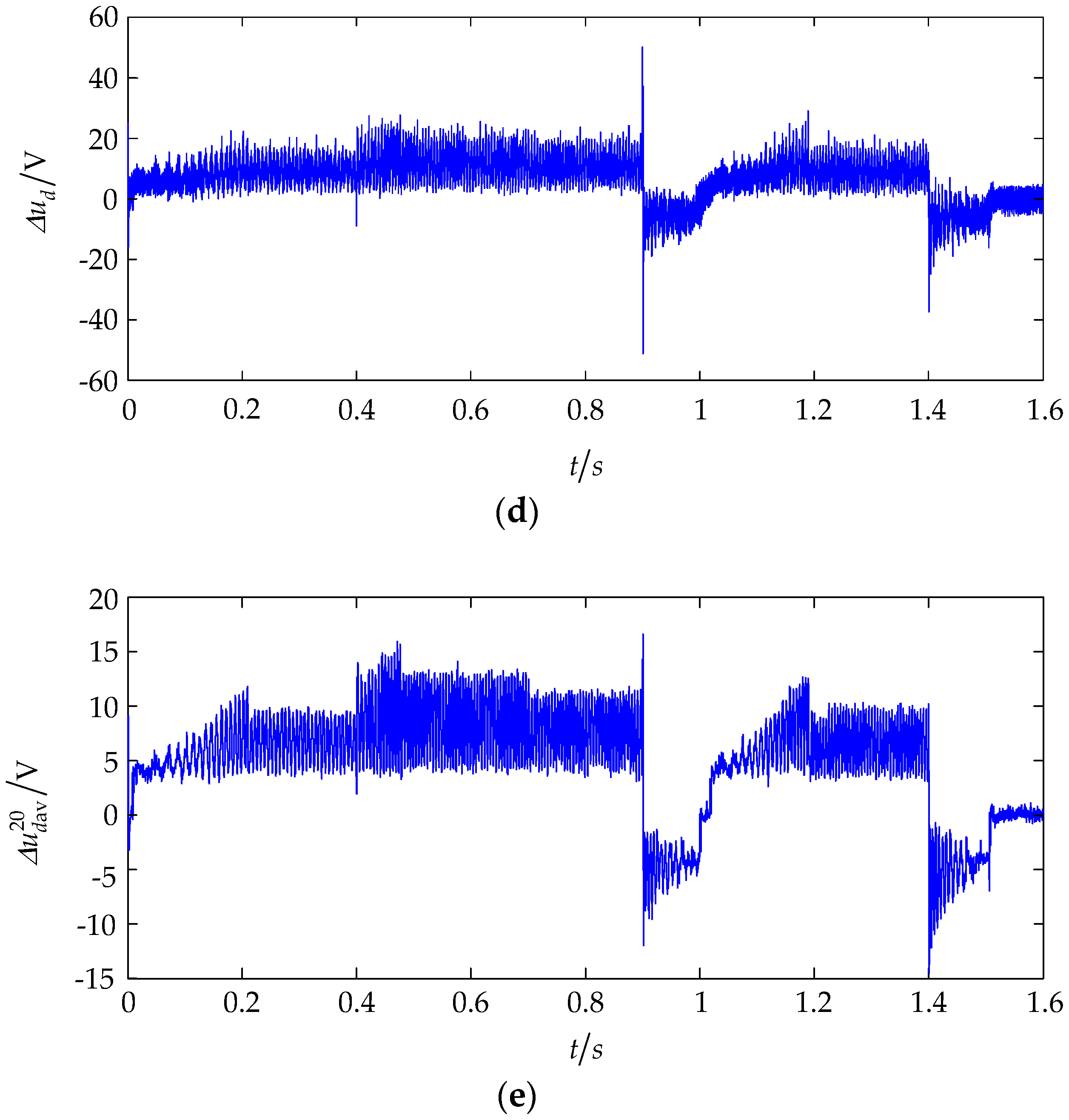
When the DRPMSM operates, it is necessary to detect ISCFs under both stationary and non-stationary conditions. When the DRPMSM has a coil ISCF under various conditions, the corresponding simulation results of the motor are shown in Figure 11. The external contact resistance and the number of short-circuited turns are set to 0.1 Ω and 10, respectively. The simulation time is 1.6 s. The reference speed and load for simulation are set as follows:

$$\{\begin{array}{lll}{n}^{\ast }=900\mathrm{r}/\min \hfill & T_{\mathrm{L}}=26.5\mathrm{N}·\mathrm{m}\hfill & \left(0\le t<0.4\mathrm{s}\right)\hfill \\ n^{\ast }=1200\mathrm{r}/\min \hfill & T_{\mathrm{L}}=26.5\mathrm{N}·\mathrm{m}\hfill & \left(0.4\le t<0.7\mathrm{s}\right)\hfill \\ n^{\ast }=1200\mathrm{r}/\min \hfill & T_{\mathrm{L}}=13.25\mathrm{N}·\mathrm{m}\hfill & \left(0.7\le t<0.9\mathrm{s}\right)\hfill \\ n^{\ast }=-1200\mathrm{r}/\min \hfill & T_{\mathrm{L}}=13.25\mathrm{N}·\mathrm{m}\hfill & \left(t\ge 0.9\mathrm{s}\mathrm{and}n>0\right)\hfill \\ n^{\ast }=-1200\mathrm{r}/\min \hfill & T_{\mathrm{L}}=-13.25\mathrm{N}·\mathrm{m}\hfill & \left(t<1.4\mathrm{s}\mathrm{and}n\le 0\right)\hfill \\ n^{\ast }=0\mathrm{r}/\min \hfill & T_{\mathrm{L}}=-13.25\mathrm{N}·\mathrm{m}\hfill & \left(1.4\le t\le 1.6\mathrm{s}\right)\hfill \end{array}$$

(61)

The whole simulation processes include the acceleration process, the stable operation process, the deceleration process and the load changing process. Except for the stable operation process, the remaining processes are all under non-stationary conditions. When the DRPMSM operates in the acceleration process or the stable process, the motor is in the motor running mode. When the DRPMSM operates in the deceleration process, the motor is in the feedback braking mode. The waveforms of the reference speed and actual speed, the reference resistant constant torque load and electromagnetic torque, the d-axis voltages of two sets of windings, $\Delta u_d$ and $\Delta u_{d\mathrm{av}}^{20}$ are all shown in Figure 11.

As shown in Figure 11, when an ISCF occurs, the actual speed of the motor can follow the reference speed. There is a longer acceleration time because the load, that is, the magnetic powder brake has a large inertia moment. In the stable operation process, the load torque and average electromagnetic torque are balanced. No matter whether the motor is rotating forward or reversely, the d-axis voltage of the set of faulty windings is greater than that of the set of normal windings in the motor running mode, except for the extremely low speed condition. $\Delta u_{d\mathrm{av}}^{20}$ change above 1 V. In the feedback braking mode, the d-axis voltage of the set of normal windings is greater than that of the set of faulty windings and $\Delta u_{d\mathrm{av}}^{20}$ change below −1 V.

In the motor running mode, $i_q$ and $\omega$ always have the same sign, so the values of $\omega i_q\Delta L$ are always positive and $\Delta u_{d\mathrm{av}}^K$ are greater than a certain positive value. In the feedback braking mode, $i_q$ and $\omega$ are opposite in sign, so $\omega i_q\Delta L$ is always negative and $\Delta u_{d\mathrm{av}}^K$ is less than a certain negative value. The positive value and the negative value mentioned above can be used as the threshold for ISCF diagnosis. Therefore, the set of faulty windings in the DRPMSM can be detected online according to the running modes and $\Delta u_{d\mathrm{av}}^K$ of the DRPMSM.

In addition, it can be ascertained from simulation results that when K is relatively small, the fluctuations of $\Delta u_{d\mathrm{av}}^K$ are relatively large, so the threshold voltage $U_{\mathrm{T}}$ for ISCF diagnosis is relatively small and the sensitivity of fault diagnosis is relatively poor. When K is relatively large, the fluctuations of $\Delta u_{d\mathrm{av}}^K$ are relatively small but the real-time performance of online detection is getting worse. Taking the above situations into account, it is appropriate to set the value of K to 20.

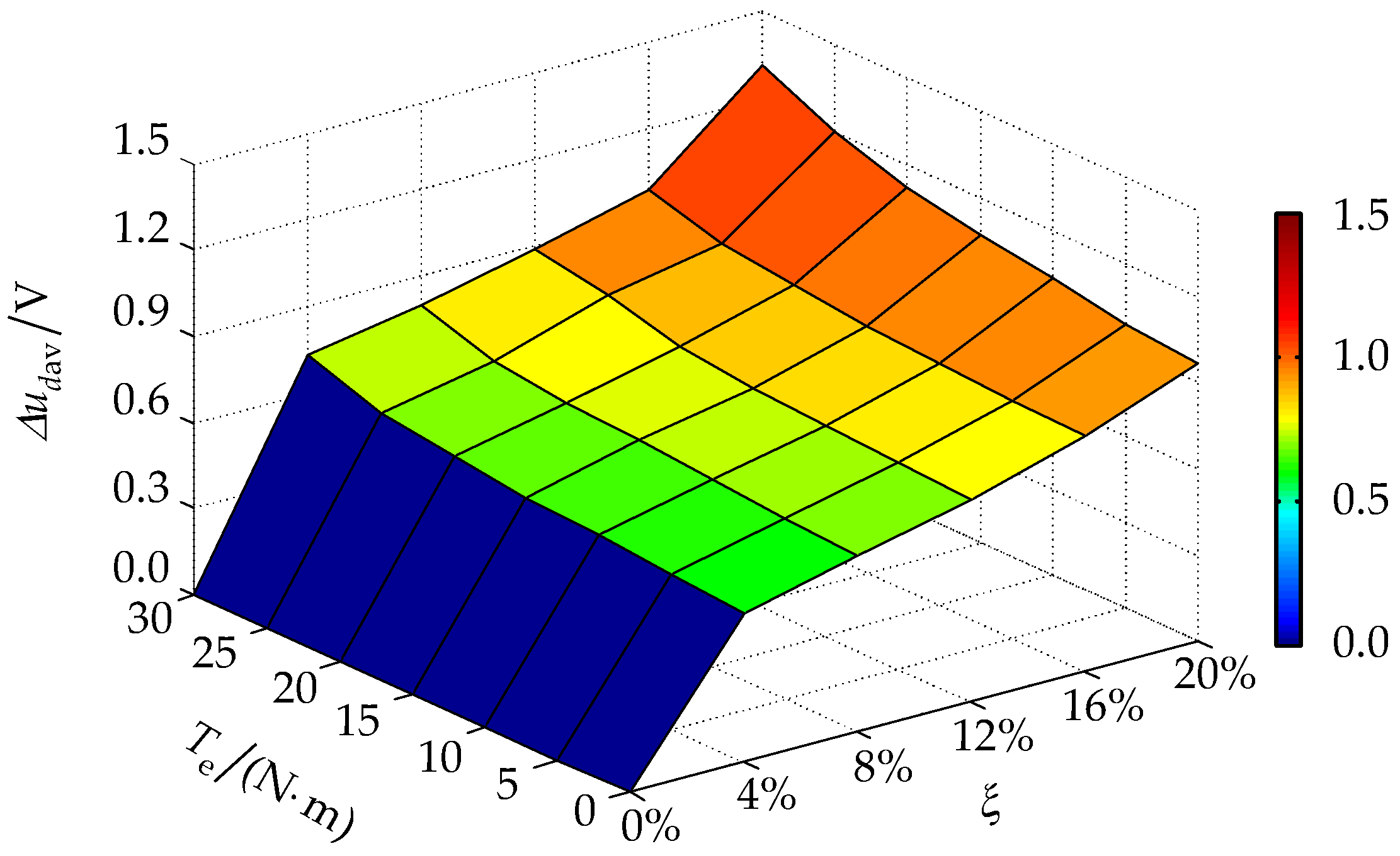
When $K\to \infty$, $\Delta u_{d\mathrm{av}}^K$ are the average values for the difference of the d-axis voltages between the set of faulty windings and the set of normal windings, that is, $\Delta u_{d\mathrm{av}}$. When the speed is 900 r/min and the external contact resistance is 0.1 Ω, the three-dimension surface curve of $\Delta u_{d\mathrm{av}}$ with the percentage for the number of short-circuited turns $\xi$ ($\xi =N_{\mathrm{s}}/N_{\mathrm{c}}$) and the electromagnetic torque is shown in Figure 12.

It can be obtained from Figure 12 that when the number of short-circuited turns is constant, $\Delta u_{d\mathrm{av}}$ will increase gradually as the electromagnetic torque increases. When the electromagnetic torque is constant, $\Delta u_{d\mathrm{av}}$ will increase gradually as the number of short-circuited turns increases.

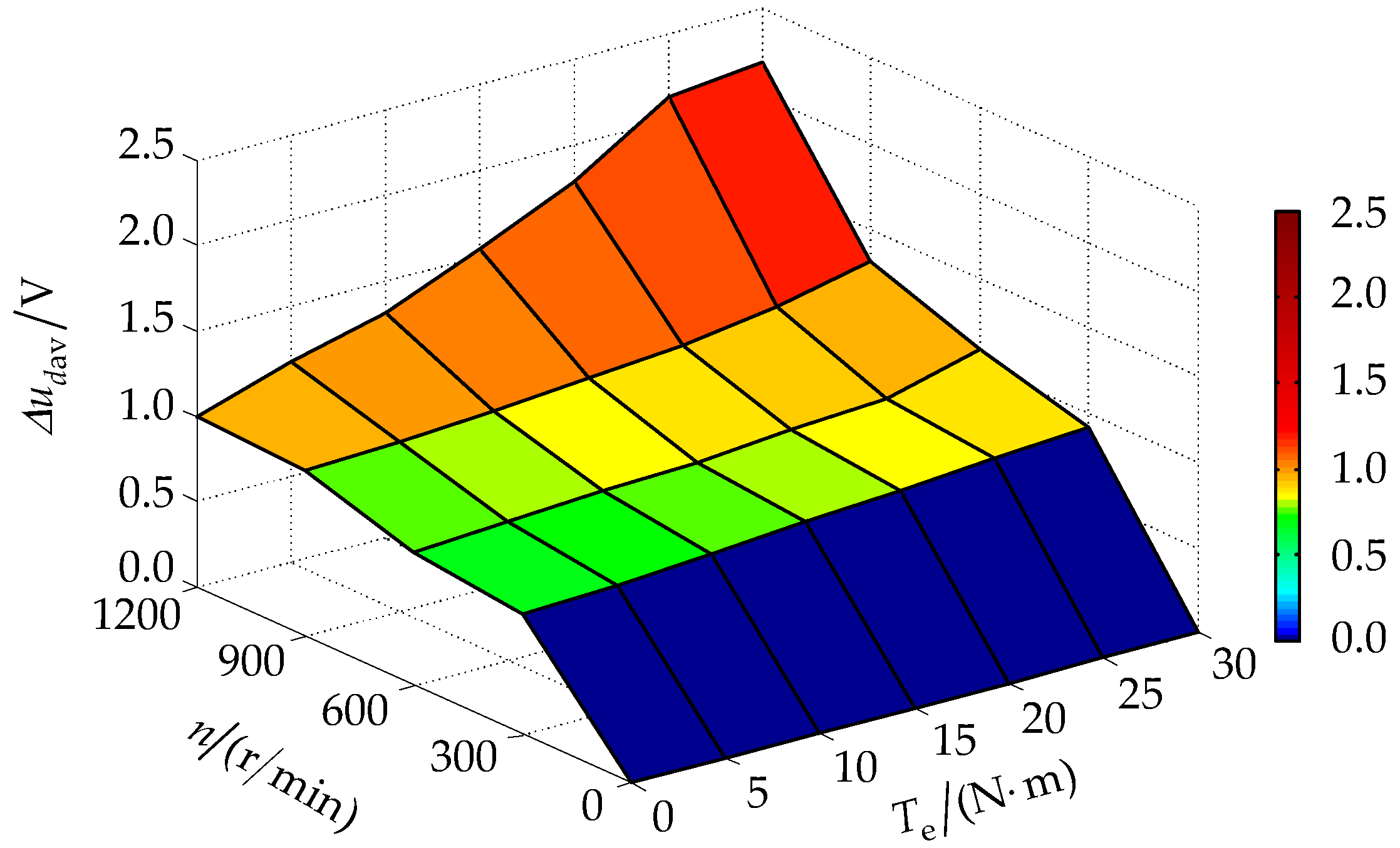
When the percentage for the number of short-circuited turns is 20% and the external contact resistance is 0.1 Ω, the three-dimension surface curve of $\Delta u_{d\mathrm{av}}$ with the electromagnetic torque and the speed is shown in Figure 13.

It can be obtained from Figure 13 that when the electromagnetic torque is constant, $\Delta u_{d\mathrm{av}}$ will increase gradually as the speed increases. When the speed is constant, $\Delta u_{d\mathrm{av}}$ will increase gradually as the electromagnetic torque increases.

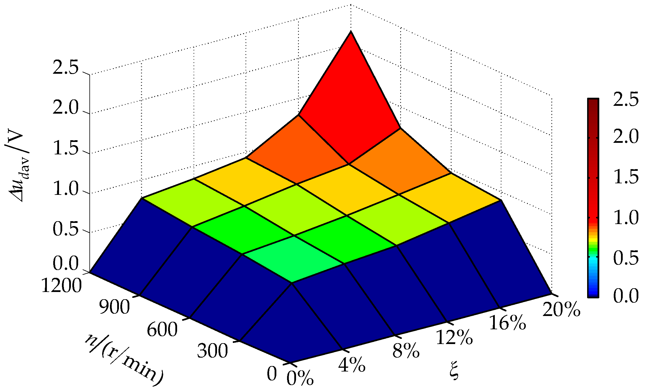
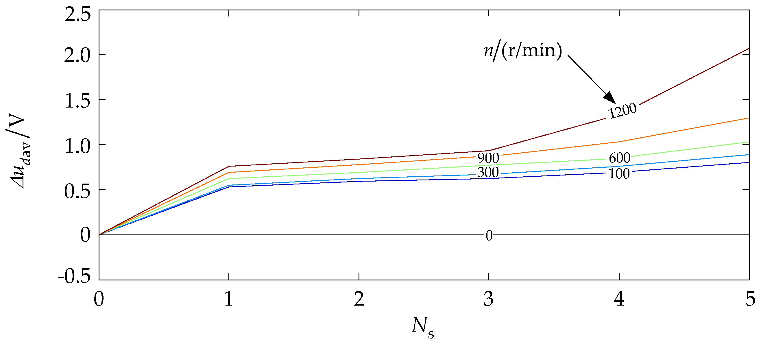
When the electromagnetic torque is the rated torque and the external contact resistance is 0.1 Ω, the three-dimension surface curve of $\Delta u_{d\mathrm{av}}$ with the percentage for the number of short-circuited turns and the speed is shown in Figure 14.

It can be obtained from Figure 14 that when the number of short-circuited turns is constant, $\Delta u_{d\mathrm{av}}$ will increase gradually as the speed increases. When the speed is constant, $\Delta u_{d\mathrm{av}}$ will increase gradually as the number of short-circuited turns increases.

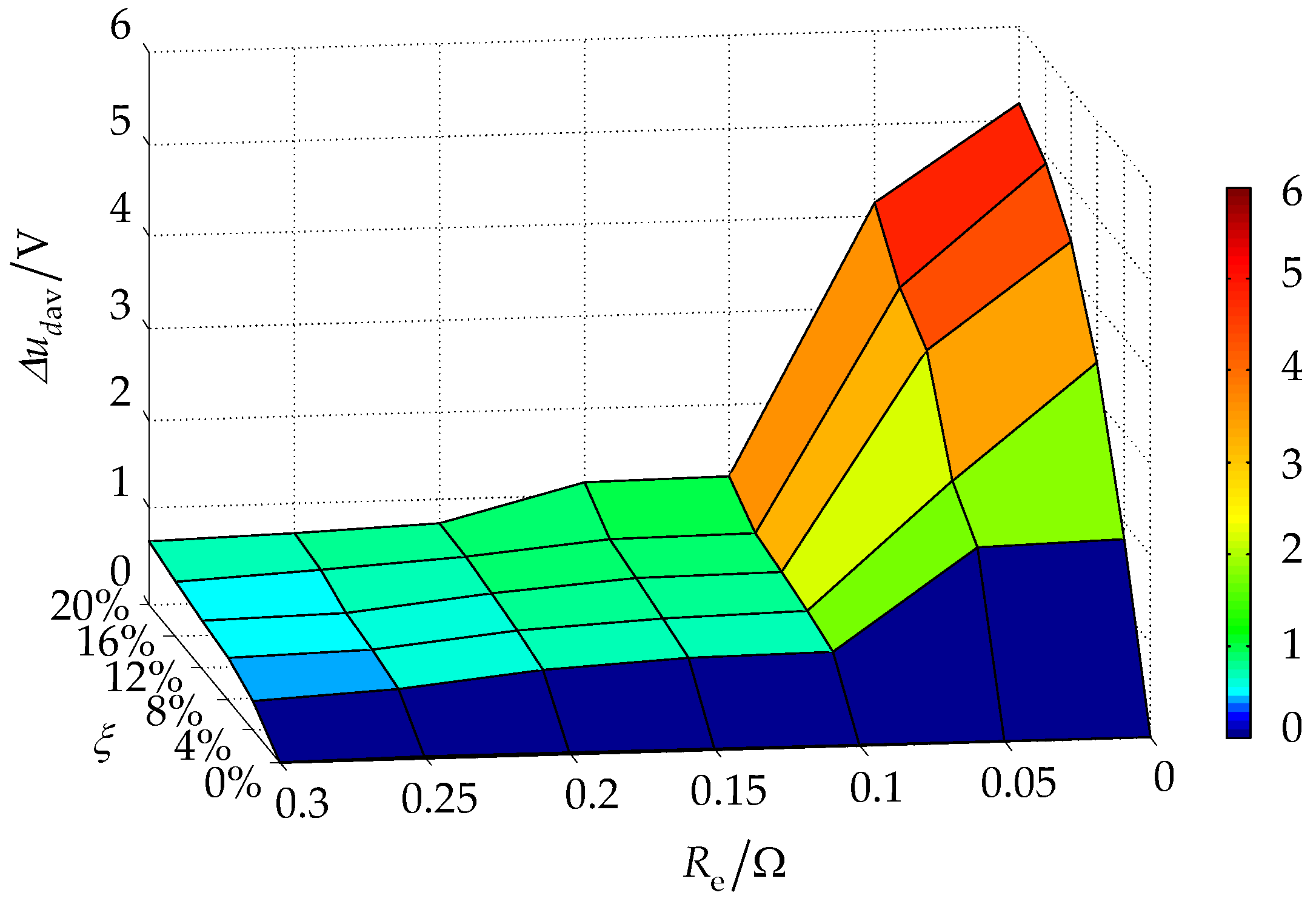
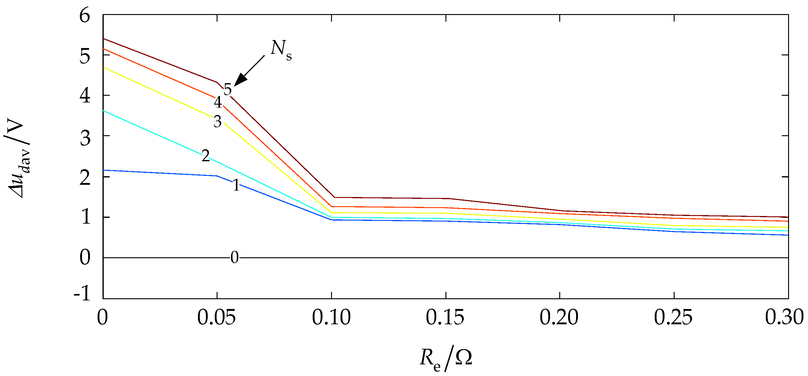
When the speed is 900 r/min and the electromagnetic torque is the rated torque, the three-dimension surface curve of $\Delta u_{d\mathrm{av}}$ with the external contact resistance and the percentage for the number of short-circuited turns is shown in Figure 15.

It can be obtained from Figure 15 that when the external contact resistance is constant, $\Delta u_{d\mathrm{av}}$ will increase gradually as the number of short-circuited turns increases. When the number of short-circuited turns is constant, $\Delta u_{d\mathrm{av}}$ will decrease gradually as the external contact resistance increases.

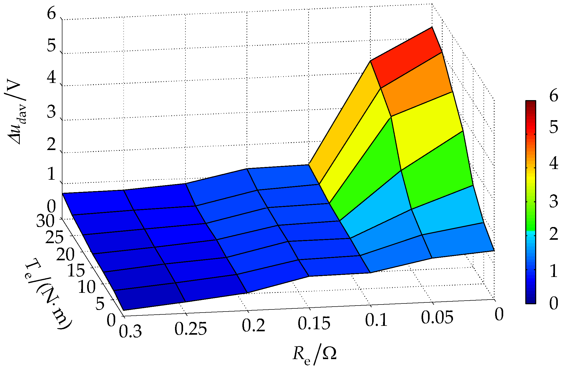
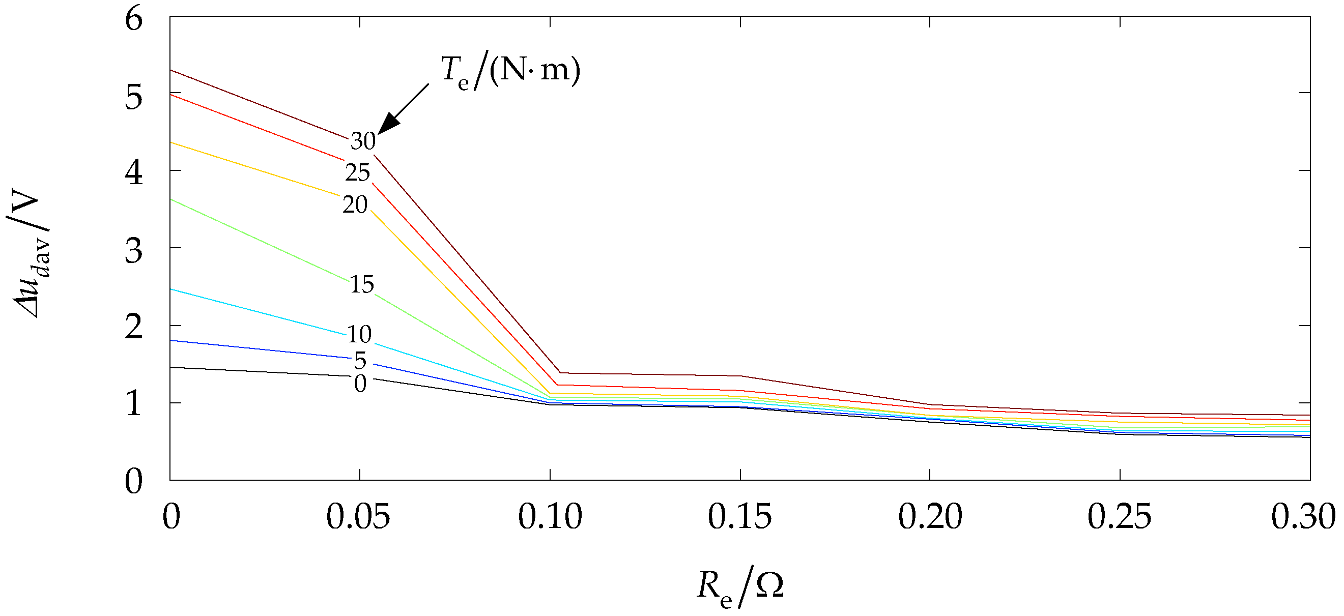
When the speed is 900 r/min and the percentage for the number of short-circuited turns is 20%, the three-dimension surface curve of $\Delta u_{d\mathrm{av}}$ with the external contact resistance and the electromagnetic torque is shown in Figure 16.

It can be obtained from Figure 16 that when the external contact resistance is constant, $\Delta u_{d\mathrm{av}}$ will increase gradually as the electromagnetic torque increases. When the electromagnetic torque is constant, $\Delta u_{d\mathrm{av}}$ will decrease gradually as the external contact resistance increases.

After an ISCF occurs, $\Delta u_{d\mathrm{av}}$ are always greater than 0.5 V when the motor runs steadily with small external contact resistance under various conditions. Similarly, when the motor runs in the feedback braking mode, $\Delta u_{d\mathrm{av}}$ are always less than −0.5 V. In addition, the above simulation results are all carried out when $\xi$ is less than or equal to 20%. When $\xi$ is greater than 20%, $\left|\Delta u_{d\mathrm{av}}\right|$ will be greater. And then, the sensitivity of the ISCF diagnosis will be higher. For the DRPMSM in this article, it is appropriate to set $U_{\mathrm{T}}$ to 0.5 V.

Combining the above theoretical analyses and the simulation results under various operating conditions, a conclusion can be obtained. That is, the DRPMSM has a coil ISCF when $\left|\Delta u_{d\mathrm{av}}^{20}\right|\ge 0.5\mathrm{V}$. Then we can determine the set of faulty windings online according to the sign of $\Delta u_{d\mathrm{av}}^{20}$ and the running modes of the DRPMSM as follows:

(1)

When $\Delta u_{d\mathrm{av}}^{20}>0.5\mathrm{V}$ and the motor operates in the motor running mode, the ISCF in the stator coil occurs in the second set of windings.

(2)

When $\Delta u_{d\mathrm{av}}^{20}>0.5\mathrm{V}$ and the motor runs in the feedback braking mode, the ISCF in the stator coil occurs in the first set of windings.

(3)

When $\Delta u_{d\mathrm{av}}^{20}<-0.5\mathrm{V}$ and the motor operates in the motor running mode, the ISCF in the stator coil occurs in the first set of windings.

(4)

When $\Delta u_{d\mathrm{av}}^{20}<-0.5\mathrm{V}$ and the motor runs in the feedback braking mode, the ISCF in the stator coil occurs in the second set of windings.

4.3. Fault Diagnosis and Redundancy Controller

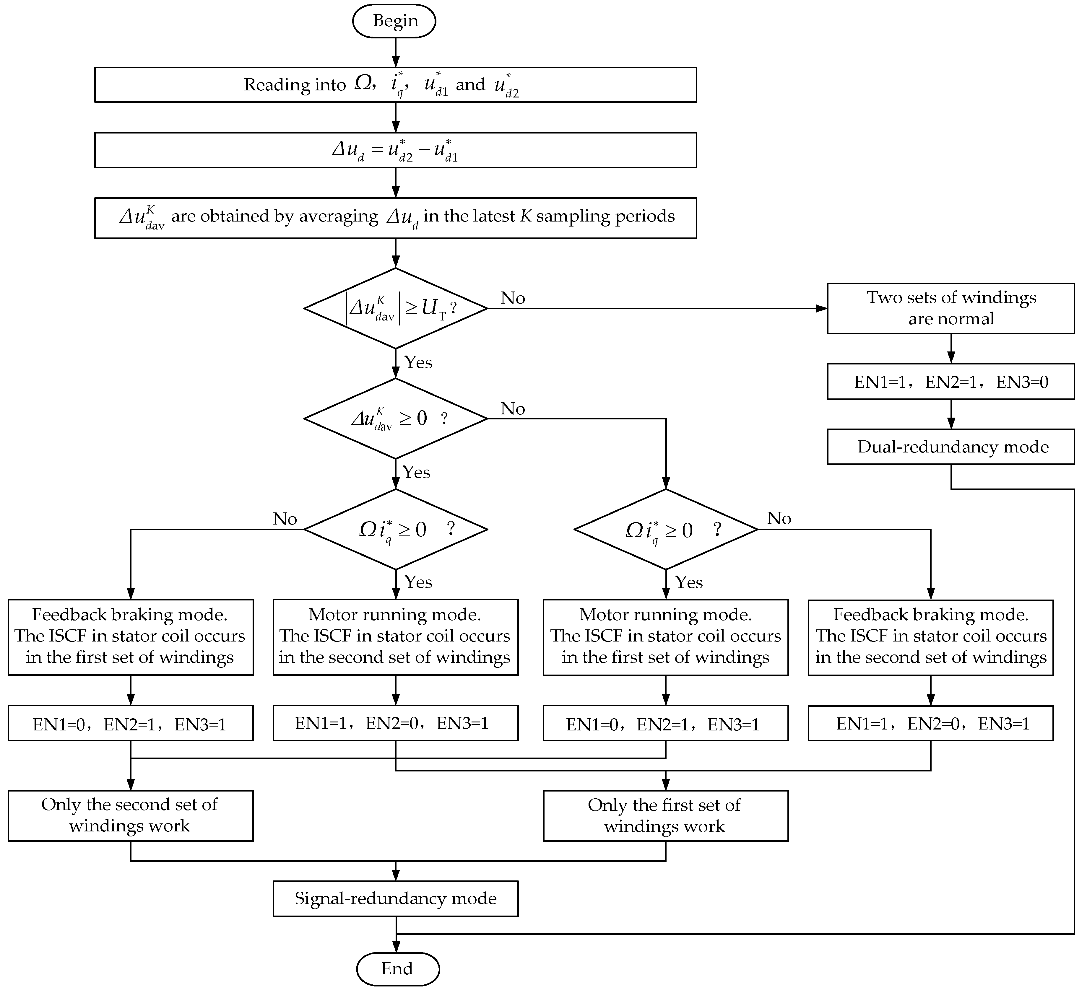
Based on the above analyses of the ISCF diagnosis method for the DRPMSM, the logic block diagram of the fault diagnosis and redundancy controller in Figure 4 can be shown in Figure 17.

EN1 and EN2 are the enable signals of the first inverter and the second inverter respectively. EN3 is the enable signal for redundancy control.

When the DRPMSM is normal, EN1 = 1, EN2 = 1, and EN3 = 0. Two inverters work simultaneously and supply power to two sets of windings, respectively. In this case, the motor operates in the dual-redundancy mode.

When the ISCF occurs in the first set of windings, EN1 = 0 and the first inverter is forbidden to supply power to the first set of windings. Similarly, when the ISCF occurs in the second set of windings, EN2 = 0 and the second inverter is forbidden to supply power to the second set of windings. Under these circumstances, the motor operates in the single-redundancy mode.

When the ISCF occurs in either set of windings, EN3 = 1 and the control strategy of the speed regulator is changed to improve the control performance of the system. For example, a frequency adaptive proportional resonant controller is paralleled with the proportional integral controller in the speed loop to suppress the electromagnetic torque ripple generated by the short-circuited coils [31].

5. Experimental Results Analyses

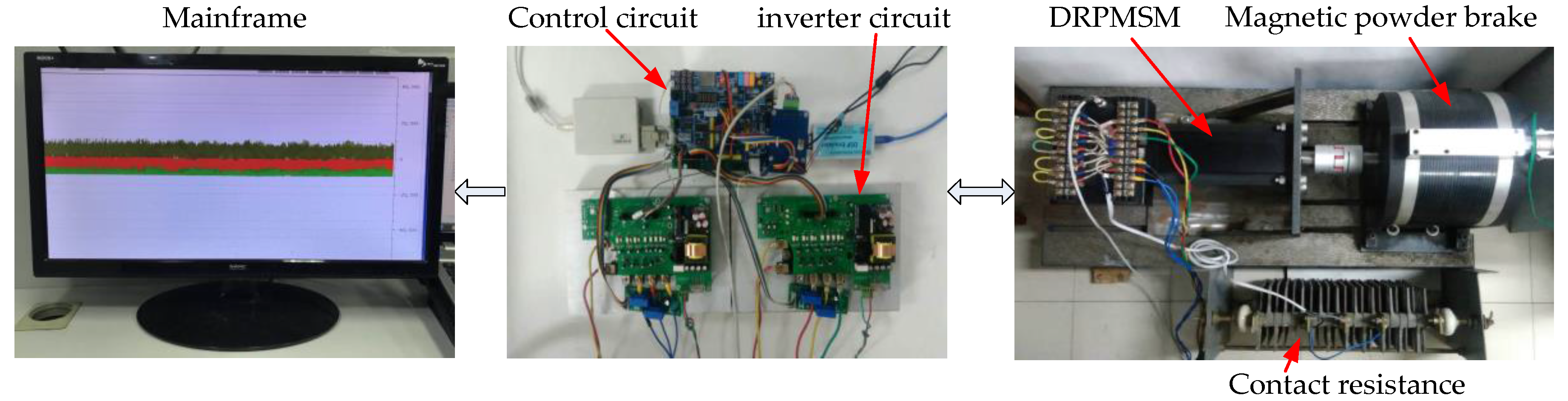
In order to verify the effectiveness of the fault detection method, the control system of the DRPMSM is built based on the DSP (TMS320F2812, Texas Instruments, Dallas, TX, USA), as shown in Figure 18. The rotor position signal is measured by a rotary transformer. Then it is converted into digital form by the decoder chip (AD2S1210, Analog Devices, Shanghai, China) and sent to the DSP. PWM signals are generated by the DSP to drive the DRPMSM.

The d-axis voltage mentioned in this paper is the output of the current regulator and is linearly related to the actual d-axis voltage. The d-axis voltage is used to calculate $\left|\Delta u_{d\mathrm{av}}^{20}\right|$, which could not only simplify the simulation and experimental model, but also improve the accuracy of the fault detection online. The average values for the difference of the d-axis voltages between two sets of windings are obtained by the DSP.

The reference speed is set to 900 r/min in the experimental system with rated load. Moreover, 10 turns of coil 12 in the C2 phase winding are shorted by an external contact resistance of 0.1 Ω. The measured current waveforms of the second set of three-phase windings are shown in Figure 19. The waveforms of the d-axis voltages of two sets of windings, $\Delta u_d$ and $\Delta u_{d\mathrm{av}}^{20}$ under normal and faulty conditions are shown in Figure 20 and Figure 21, respectively.

As shown in Figure 19, when the DRPMSM is in normal state, the three-phase current waveforms are symmetric sine waves. After ISCF occurs, the three-phase current waveforms are distorted, and the amplitude of the current increases to generate larger electromagnetic torque for compensating the braking torque generated by short-circuited turns. Thus, the output average electromagnetic torque remains constant.

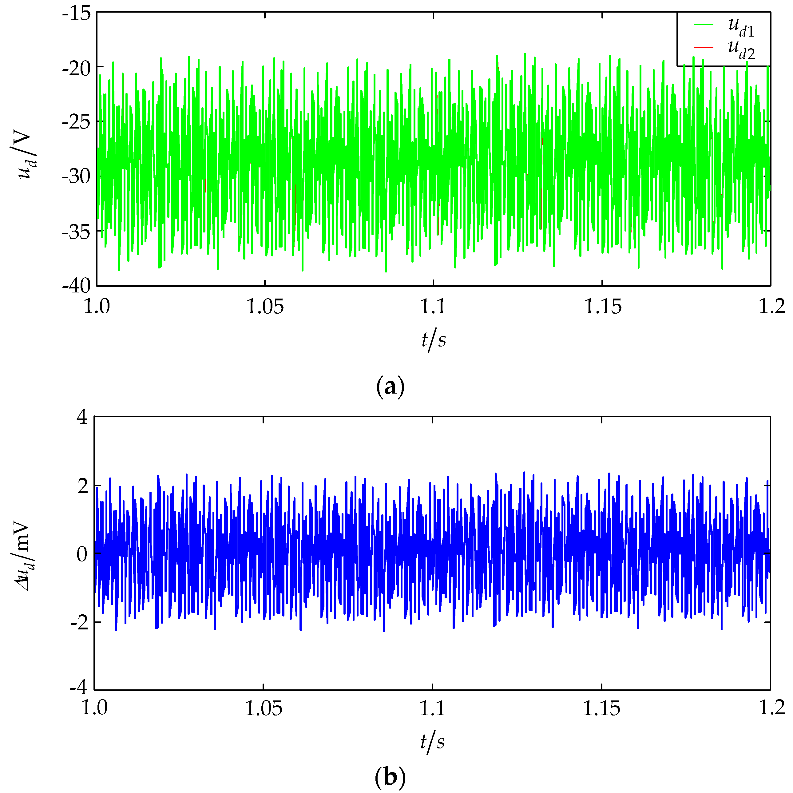
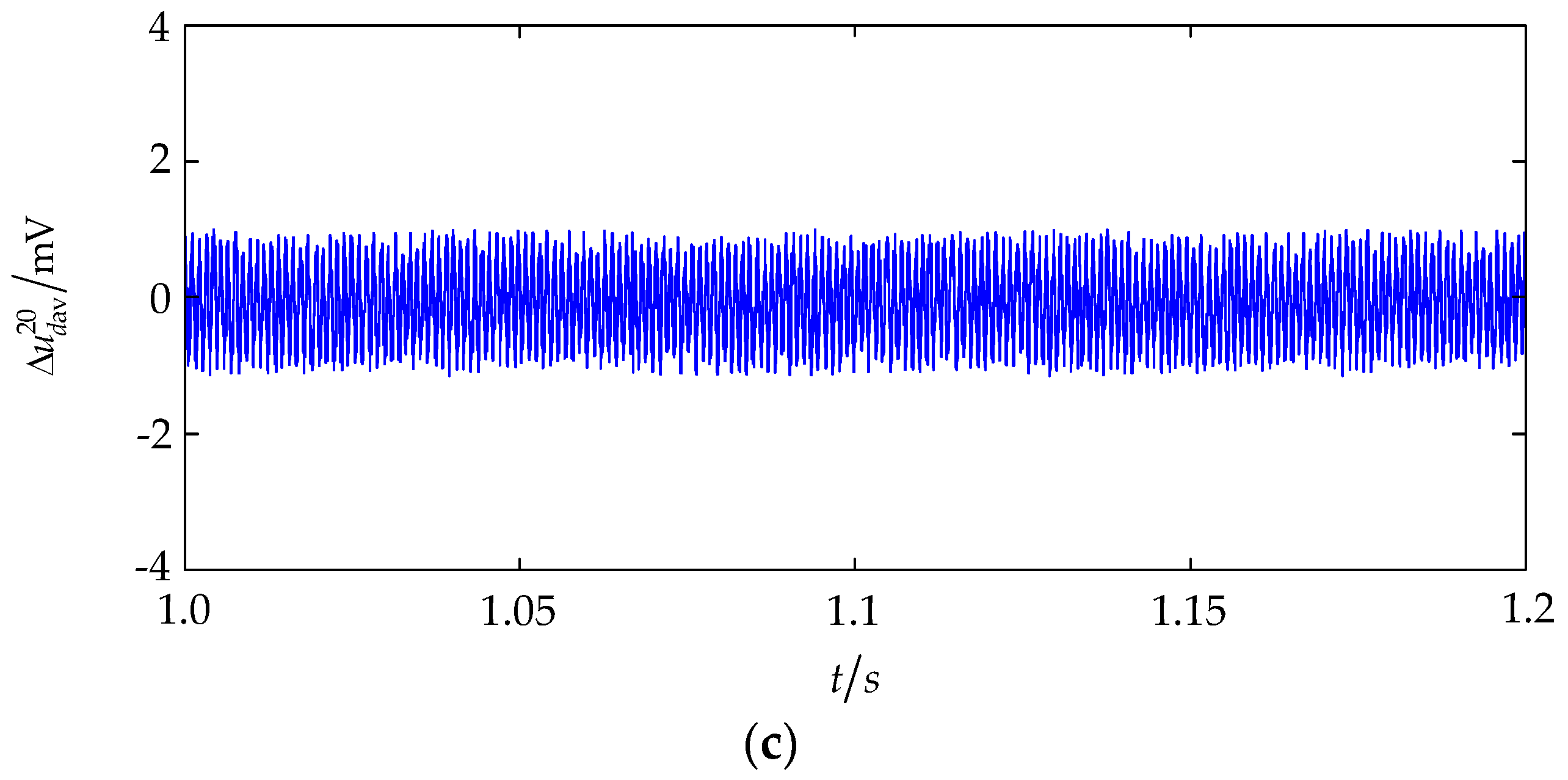
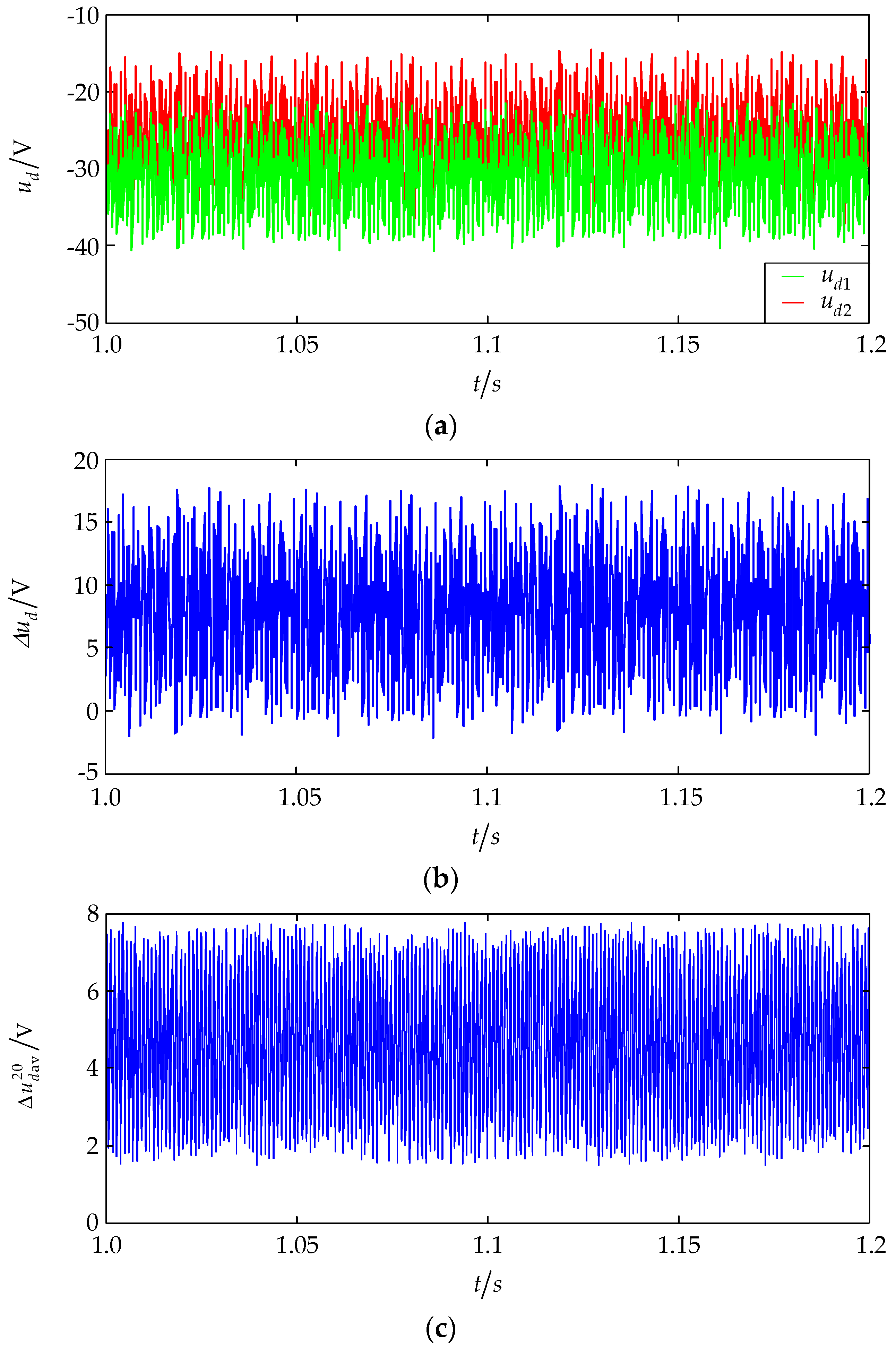
As shown in Figure 20 and Figure 21, when the motor runs normally, the d-axis voltages of two sets of windings are basically the same, $\Delta u_d$ and $\Delta u_{d\mathrm{av}}^{20}$ fluctuate within ±2 mV and ±1 mV, respectively. When an ISCF occurs, the d-axis voltage of the set of faulty windings is much higher than that of the set of normal windings. Further, $\Delta u_d$ are basically positive, the maximum value and the minimum value of $\Delta u_d$ are about 18 V and –2 V. So all the $\Delta u_{d\mathrm{av}}^{20}$ change above 1 V.

When the speed is 900 r/min and the external contact resistance is 0.1 Ω, the variation curves of $\Delta u_{d\mathrm{av}}$ with the number of short-circuited turns and the electromagnetic torque is shown in Figure 22.

It can be obtained from Figure 22 that when the DRPMSM is normal, $\Delta u_{d\mathrm{av}}$ is 0 V. When an ISCF occurs, $\Delta u_{d\mathrm{av}}$ change above 0.5 V under any electromagnetic torque and relatively few the number of short-circuited turns.

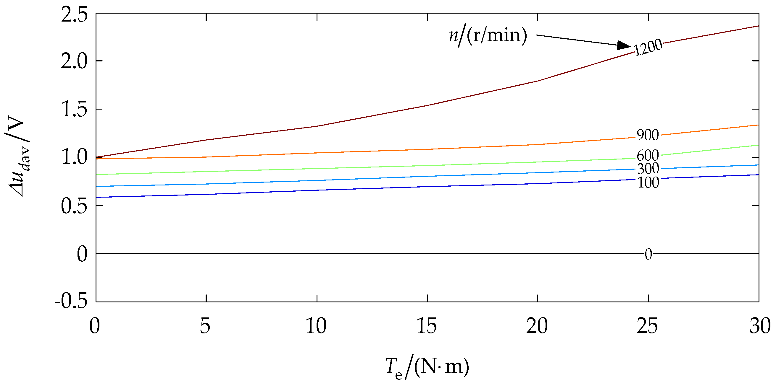
When the number of short-circuited turns is 5 and the external contact resistance is 0.1 Ω, the variation curves of $\Delta u_{d\mathrm{av}}$ with the speed and the electromagnetic torque is shown in Figure 23.

It can be obtained from Figure 23 that when an ISCF occurs, $\Delta u_{d\mathrm{av}}$ change above 0.5 V under various speeds and electromagnetic torques.

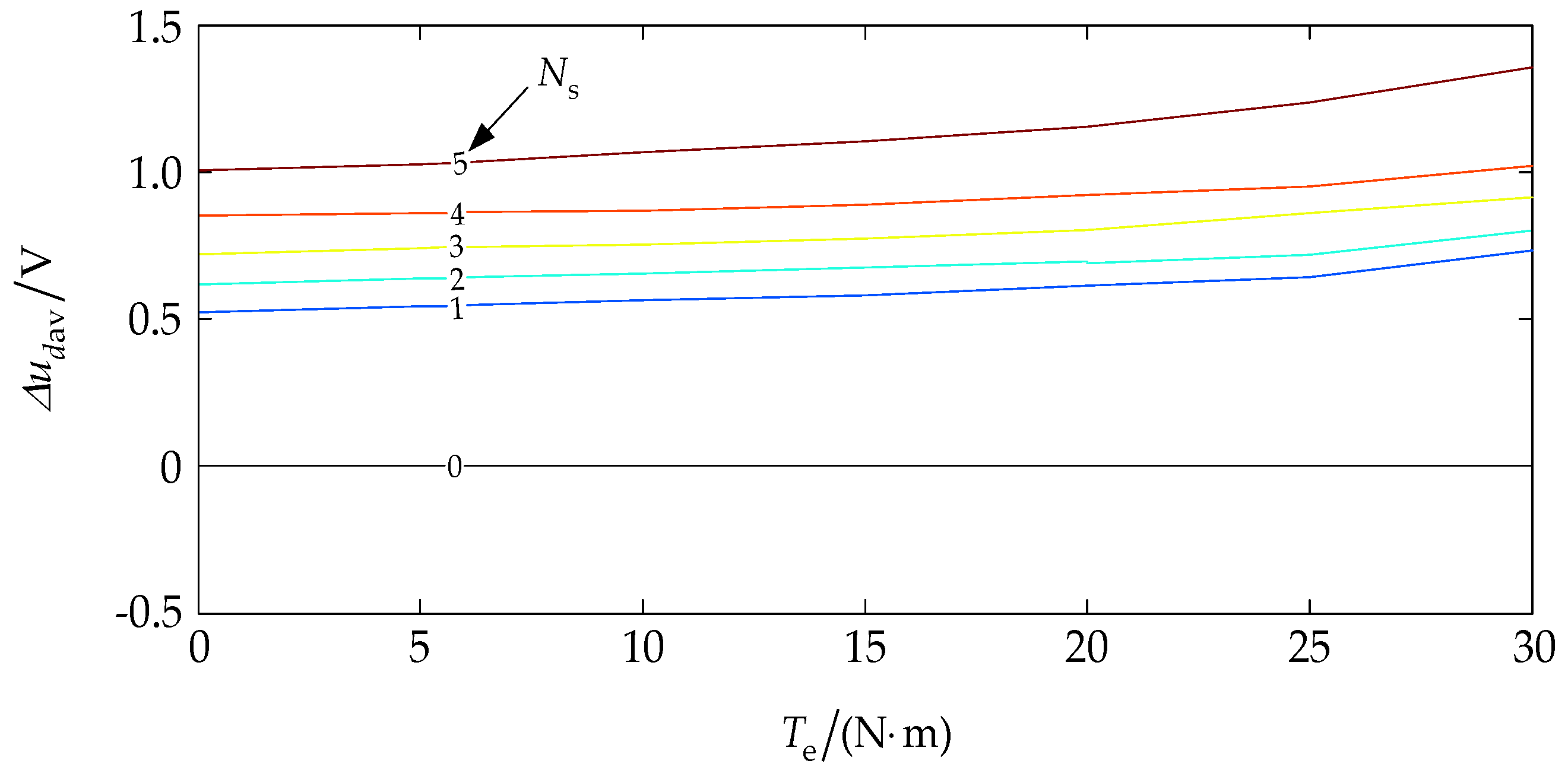
When the electromagnetic torque is the rated torque and the external contact resistance is 0.1 Ω, the variation curves of $\Delta u_{d\mathrm{av}}$ with the speed and the number of short-circuited turns is shown in Figure 24.

It can be obtained from Figure 24 that when an ISCF occurs, $\Delta u_{d\mathrm{av}}$ change above 0.5 V under various speeds and relatively few the number of short-circuited turns.

When the speed is 900 r/min and the electromagnetic torque is the rated torque, the variation curves of $\Delta u_{d\mathrm{av}}$ with the number of short-circuited turns and the external contact resistance is shown in Figure 25.

It can be obtained from Figure 25 that when the DRPMSM is normal, $\Delta u_{d\mathrm{av}}$ is 0 V. When an ISCF occurs, $\Delta u_{d\mathrm{av}}$ change above 0.5 V under relatively few the number of short-circuited turns and relatively small external contact resistance.

When the speed is 900 r/min and the number of short-circuited turns is 5, the variation curves of $\Delta u_{d\mathrm{av}}$ with the electromagnetic torque and the external contact resistance is shown in Figure 26.

It can be obtained from Figure 26 that when an ISCF occurs, $\Delta u_{d\mathrm{av}}$ change above 0.5 V under any electromagnetic torque and relatively small external contact resistance.

Based on the above experimental results for the ISCFs of the DRPMSM under various conditions, it can be verified that 0.5 V can be used as a threshold voltage for diagnosing ISCFs and the set of faulty windings. In addition, it can be seen that the experimental results are basically consistent with the simulation results.

6. Conclusions

In this paper, the diagnosis method of ISCFs in DRPMSMs is analyzed. Firstly, the structure of the motor is analyzed. Secondly, the calculation formulas for the inductance of each part of the stator winding are deduced, the mathematical models of the motor are established in MATLAB/Simulink, and then the ISCF of the motor is simulated and analyzed. Finally, according to the running modes of the DRPMSM and the average values for the difference of the d-axis voltages between two sets of windings in the latest 20 sampling periods, the ISCF and the set of faulty windings can be diagnosed online. The main conclusions are as follows:

(1)

After an ISCF occurs, the structures and permanent magnet back EMFs of two sets of windings both change. Nevertheless, the control systems of two sets of windings are controlled by one speed regulator, that is, the inputs of current regulators of two sets of windings are the same. Besides, the adjusting speed of current regulator is extremely fast, so the three phase currents of two sets of windings produce nearly the same distortion. Thus, according to the currents of two sets of windings, the ISCF can be diagnosed. However, it is impossible to determine the set of faulty windings.

(2)

After an ISCF occurs, the impedance of the set of faulty windings reduces, thus the absolute value for the d-axis voltage of the set of faulty windings becomes smaller. According to the equation for the d-axis voltage of the PMSM in a synchronous rotating frame, when the motor runs in the motor running mode, the d-axis voltage is negative while the average values for the difference of the d-axis voltages between the set of faulty windings and the set of normal windings are positive. When the motor runs in the feedback braking mode, the d-axis voltage is positive while the average values for the difference of the d-axis voltages between the set of faulty windings and the set of normal windings are negative. Therefore, the ISCF and the set of faulty windings of the DRPMSM can be detected online by analyzing the running modes of the DRPMSM and the average values for the difference of the d-axis voltages between two sets of windings in the latest 20 sampling periods.

(3)

The average values for the difference of the d-axis voltages between the set of faulty windings and the set of normal windings are relevant to the number of short-circuited turns, the external contact resistance, the load, the speed and the running modes of the DRPMSM.

To sum up, the proposed method is feasible for detecting an ISCF and the set of faulty windings of the DRPMSM online. After diagnosing the set of faulty windings of the DRPMSM, removing the set of faulty windings timely could improve the reliability of the motor.

References

- Tian, Z.; Zhang, C.; Zhang, S. Analytical calculation of magnetic field distribution and stator iron losses for surface-mounted permanent magnet synchronous machines. Energies 2017, 10, 320. [Google Scholar] [CrossRef]
- Yan, H.; Xu, Y.X.; Zou, J.B. A phase current reconstruction approach for three-phase permanent-magnet synchronous motor drive. Energies 2016, 9, 853. [Google Scholar] [CrossRef]
- Zhao, J.; Li, B.; Gu, Z.X. Research on an axial flux PMSM with radially sliding permanent magnets. Energies 2015, 8, 1663–1684. [Google Scholar] [CrossRef]
- An, Q.T.; Liu, J.; Peng, Z.; Sun, L.; Sun, L.Z. Dual-space vector control of open-end windings permanent magnet synchronous motor drive fed by dual inverter. IEEE Trans. Power Electron. 2016, 31, 8329–8342. [Google Scholar] [CrossRef]
- Yang, J.W.; Dou, M.F.; Dai, Z.Y. Modeling and fault diagnosis of interturn short circuit for five-phase permanent magnet synchronous motor. J. Electr. Comput. Eng. 2015, 2015, 168786. [Google Scholar] [CrossRef]
- Shen, Y.H.; Zhou, X.; Chen, Y.G. A new instantaneous sequence component analysis of double-redundancy permanent magnet synchronous motor based on field-circuit coupling. In Proceedings of the 2016 19th International Conference on Electrical Machines and Systems (ICEMS), Chiba, Japan, 13–16 November 2016; pp. 1–6. [Google Scholar]
- Chen, Y.G.; Zhai, W.C.; Shen, Y.H. Analysis on temperature field distribution of dual-redundancy PMSM. J. Tianjin Univ. 2015, 48, 488–493. [Google Scholar] [CrossRef]
- Wu, F.; Tong, C.D.; Sui, Y.; Cheng, L.M.; Zheng, P. Influence of third harmonic back EMF on modeling and remediation of winding short circuit in a multiphase PM machine with FSCWs. IEEE Trans. Ind. Electron. 2016, 63, 6031–6041. [Google Scholar] [CrossRef]
- Zhang, C.F.; Luo, L.X.; He, J.; Liu, N. Analysis of the short-circuit fault characteristics of permanent magnet synchronous machines. In Proceedings of the 2015 Chinese Automation Congress (CAC), Wuhan, China, 27–29 November 2015; pp. 1913–1917. [Google Scholar]
- Sjökvist, S.; Eriksson, S. Investigation of permanent magnet demagnetization in synchronous machines during multiple short-circuit fault conditions. Energies 2017, 10, 1638. [Google Scholar] [CrossRef]
- Mazzoletti, M.A.; Bossio, G.R.; Angelo, C.H.D.; Espinoza-Trejo, D.R. A model-based strategy for interturn short-circuit fault diagnosis in PMSM. IEEE Trans. Ind. Electron. 2017, 64, 7218–7228. [Google Scholar] [CrossRef]
- Duvvuri, S.S.S.R.S.; Detroja, K. Model-based stator interturn short-circuit fault detection and diagnosis in induction motors. In Proceedings of the 2015 7th International Conference on Information Technology and Electrical Engineering (ICITEE), Chiang Mai, Thailand, 29–30 October 2015; pp. 167–172. [Google Scholar]
- Ogidi, O.O.; Barendse, P.S.; Khan, M.A. The detection of interturn short circuit faults in axial-flux permanent magnet machine with concentrated windings. In Proceedings of the 2015 IEEE Energy Conversion Congress and Exposition (ECCE), Montreal, QC, Canada, 20–24 September 2015; pp. 1810–1817. [Google Scholar]
- Du, B.C.; Wu, S.P.; Han, S.L.; Cui, S.M. Interturn fault diagnosis strategy for interior permanent-magnet synchronous motor of electric vehicles based on digital signal processor. IEEE Trans. Ind. Electron. 2016, 63, 1694–1706. [Google Scholar] [CrossRef]
- Fitouri, M.; Bensalem, Y.; Abdelkrim, M.N. Modeling and detection of the short-circuit fault in PMSM using finite element analysis. IFAC PapersOnline 2016, 49, 1418–1423. [Google Scholar] [CrossRef]
- Chen, Y.; Wang, L.L.; Wang, Z.H.; Rehman, A.U.; Cheng, Y.H.; Zhao, Y.; Tanaka, T. FEM simulation and analysis on stator winding inter-turn fault in DFIG. In Proceedings of the 2015 IEEE 11th International Conference on the Properties and Applications of Dielectric Materials (ICPADM), Sydney, NSW, Australia, 19–22 July 2015; pp. 244–247. [Google Scholar]
- Jeong, H.; Moon, S.; Kim, S.W. An early stage interturn fault diagnosis of PMSMs by using negative-sequence components. IEEE Trans. Ind. Electron. 2017, 64, 5701–5708. [Google Scholar] [CrossRef]
- Zheng, A.P.; Yang, J.; Wang, L. Fault detection of stator winding interturn short circuit in PMSM based on wavelet packet analysis. In Proceedings of the 2013 Fifth International Conference on Measuring Technology and Mechatronics Automation, Hong Kong, China, 16–17 January 2013; pp. 566–569. [Google Scholar]
- Dash, R.N.; Subudhi, B.; Das, S. Induction motor stator inter-turn fault detection using wavelet transform technique. In Proceedings of the 2010 5th International Conference on Industrial and Information Systems, Mangalore, India, 29 July–1 August 2010; pp. 436–441. [Google Scholar]
- Wang, X.H.; Chen, Y.; Peng, J.C. A new method for on-line detecting inter-turn short circuit in stator winding of AC machine. High Volt. Eng. 2003, 29, 28–30. [Google Scholar] [CrossRef]
- Bouslimani, S.; Drid, S.; Chrifi-Alaoui, L.; Bussy, P.; Hamzaoui, M. Inter-turn faults detection using Park vector strategy. In Proceedings of the 2016 17th International Conference on Sciences and Techniques of Automatic Control and Computer Engineering (STA), Sousse, Tunisia, 19–21 December 2016; pp. 244–248. [Google Scholar]
- Kim, K.H. Simple online fault detecting scheme for short-circuited turn in a PMSM through current harmonic monitoring. IEEE Trans. Ind. Electron. 2011, 58, 2565–2568. [Google Scholar] [CrossRef]
- Lee, J.; Moon, S.; Jenog, H.; Kim, S.W. Robust diagnosis method based on parameter estimation for an interturn short-circuit fault in multipole PMSM under high-speed operation. Sensors 2015, 15, 29452–29466. [Google Scholar] [CrossRef] [PubMed]
- Sun, Y.G.; Yu, X.W.; Wei, K.; Huang, Z.G.; Wang, X.Y. A new type of search coil for detecting inter-turn faults in synchronous machines. Proc. CSEE 2014, 34, 917–924. [Google Scholar] [CrossRef]
- Urresty, J.C.; Riba, J.R.; Romeral, L. Application of the zero-sequence voltage component to detect stator winding inter-turn faults in PMSMs. Electr. Power Syst. Res. 2012, 89, 38–44. [Google Scholar] [CrossRef]
- Saavedra, H.; Urresty, J.C.; Riba, J.R.; Romeral, L. Detection of interturn faults in PMSMs with different winding configurations. Energy Convers. Manag. 2014, 79, 534–542. [Google Scholar] [CrossRef]
- Barendse, P.S.; Pillay, P. A new algorithm for the detection of faults in permanent magnet machines. In Proceedings of the IECON 2006 32nd Annual Conference on IEEE Industrial Electronics, Paris, France, 6–10 November 2006; pp. 823–828. [Google Scholar]
- Bessam, B.; Menacer, A.; Boumehraz, M.; Cherif, H. A novel method for induction motors stator inter-turn short circuit fault diagnosis based on wavelet energy and neural network. In Proceedings of the 2015 IEEE 10th International Symposium on Diagnostics for Electrical Machines, Power Electronics and Drives (SDEMPED), Guarda, Portugal, 1–4 September 2015; pp. 143–149. [Google Scholar]
- Barendse, P.S.; Herndler, B.; Khan, M.A.; Pillay, P. The application of wavelets for the detection of inter-turn faults in induction machines. In Proceedings of the 2009 IEEE International Electric Machines and Drives Conference, Miami, FL, USA, 3–6 May 2009; pp. 1401–1407. [Google Scholar]
- Chen, Y.G. Inductance calculation of permanent magnet synchronous machines with fractional-slot concentrated winding. Trans. China Eletrotech. Soc. 2014, 29, 119–124. [Google Scholar] [CrossRef]
- Chen, Y.G.; Zhang, B. Minimization of the electromagnetic torque ripple caused by the coils inter-turn short circuit fault in dual-redundancy permanent magnet synchronous motors. Energies 2017, 10, 1798. [Google Scholar] [CrossRef]
Figure 1.
The cross-sectional view of the DRPMSM.
Figure 2.
The star graph of the fundamental EMF and the diagram of phase separation: (a) The star graph of the fundamental EMF; (b) The diagram of phase separation.
Figure 3.
Stator windings outspread diagram of the DRPMSM.
Figure 4.
The control system block diagram of the DRPMSM.
Figure 5.
The MMF of the C2 phase winding under normal conditions: (a) The stator winding outspread diagram; (b) The distribution diagram of the MMF generated by .
Figure 6.
The MMF of the C2 phase winding with ISCF: (a) The stator winding outspread diagram of the DRPMSM; (b) The distribution diagram of the MMF generated by ; (c) The distribution diagram of the MMF generated by .
Figure 7.
The shape of the stator slots.
Figure 8.
The equivalent circuit diagram of the second set of windings.
Figure 9.
The simulation models of an ISCF in the DRPMSM: (a) The simulation model of the overall control system for the motor; (b) The sub-model of the vector control system; (c) The sub-model of the DRPMSM; (d) The sub-model of the set of faulty windings.
Figure 10.
The simulation results (rated load, ): (a) The three phase currents of two sets of windings; (b) The electromagnetic torque; (c) The d-axis voltages of two sets of windings; (d) The difference of the d-axis voltages between the set of faulty windings and the set of normal windings; (e) The average values for the difference of the d-axis voltages in the latest 20 sampling periods.
Figure 11.
The simulation results with a coil ISCF under various operation conditions: (a) The reference speed and the actual speed; (b) The reference load torque and the electromagnetic torque; (c) The d-axis voltages of two sets of windings; (d) ; (e) .
Figure 12.
The variation diagram of with the percentage for the number of short-circuited turns and the electromagnetic torque.
Figure 13.
The variation diagram of with the electromagnetic torque and the speed.
Figure 14.
The variation diagram of with the percentage for the number of short-circuited turns and the speed.
Figure 15.
The variation diagram of with the external contact resistance and the percentage for the number of short-circuited turns.
Figure 16.
The variation diagram of with the external contact resistance and the electromagnetic torque.
Figure 17.
The logic block diagram of the fault diagnosis and redundancy controller.
Figure 18.
The experimental system diagram of the DRPMSM.
Figure 19.
The current waveforms of the second set of windings: (a) Three phase currents under normal conditions; (b) Three phase currents under faulty conditions.
Figure 20.
The waveforms about the d-axis voltage under normal conditions: (a) The d-axis voltages of two sets of windings; (b) ; (c) .
Figure 21.
The waveforms about the d-axis voltage under faulty conditions: (a) The d-axis voltages of two sets of windings; (b) ; (c) .
Figure 22.
The variation curves of with the number of short-circuited turns and the electromagnetic torque.
Figure 23.
The variation curves of with the speed and the electromagnetic torque.
Figure 24.
The variation curves of with the speed and the number of short-circuited turns.
Figure 25.
The variation curves of with the number of short-circuited turns and the external contact resistance.
Figure 26.
The variation curves of with the electromagnetic torque and the external contact resistance.